Ballistic magnetic thermal transport coupled to phonons

Abstract

Motivated by thermal conductivity experiments in spin chain compounds, we propose a phenomenological model to account for a ballistic magnetic transport coupled to a diffusive phononic one, along the line of the seminal two-temperature diffusive transport Sanders-Walton model. Although the expression for the effective thermal conductivity is identical to that of Sanders-Walton, the interpretation is entirely different, as the ”magnetic conductivity” is replaced by an ”effective transfer conductivity” between the magnetic and phononic component. This model also reveals the fascinating possibility of visualizing the ballistic character of magnetic transport, for appropriately chosen material parameters, as a two peak counter-propagating feature in the phononic temperature. It is also appropriate for the analysis of any thermal transport experiment involving a diffusive component coupled to a ballistic one.

The thermal transport by magnetic excitations has been extensively studied over the last few years hess and it was established as a novel thermal conduction mechanism besides the well known electronic and phononic ones. In particular, it was studied in one dimensional quantum magnets ballistic where it was shown that, in compounds accurately described by the Heisenberg spin-1/2 chain model, there is a ballistic magnetic component of thermal transport znp interacting with the phononic one.

Besides steady state studies of the thermal conductivity, the flash methodparker provides information on the dynamic (in time) propagation of heat and in particular on the interaction between the magnetic and phononic components flash . These studies could provide a playground for confronting experiments to recent theoretical developments on the far-out of equilibrium dynamics in integrable spin Hamiltonians ghd .

However, the magnetic excitations in a quantum magnet are interacting with the phonons and disentangling their contribution in the total thermal conductivity is an important issue. A minimal phenomenological framework of thermal conduction in a diffusive magnon plus phonon system was proposed by Sanders and Walton (SW) sw and it has become the standard model for analyzing magnetic thermal transport experiments ott . In the SW model the magnetic subsystem is assumed diffusive so it is interesting to revisit this model in the case of a ballistic magnetic component more appropriate for the spin-1/2 Heisenberg chain compounds and not only. In the following we will try to highlight the differences in the expected effective thermal conductivity and thermal pulse propagation between the two models, namely the two-temperature SW diffusion model and the present advection-diffusion one.

In SW the starting relation is the equilibration in time of the phonon ($T_{p}$) and magnetic ($T_{m}$) temperature difference,

$$\frac{\partial\Delta T}{\partial t}=-\frac{\Delta T}{\tau},~{}~{}~{}\Delta T=T_{p}-T_{m}$$ (1)

where $\tau$ is a characteristic phenomenological relaxation time. This basic relation is also satisfied by a system of individual contributions,

$$\frac{\partial T_{p}}{\partial t} = \frac{c_{m}}{C}\frac{T_{m}-T_{p}}{\tau}$$

$$\frac{\partial T_{+}}{\partial t} = \frac{c_{p}}{C}\frac{T_{p}-T_{+}}{\tau}$$

$$\frac{\partial T_{-}}{\partial t} = \frac{c_{p}}{C}\frac{T_{p}-T_{-}}{\tau},$$ (2)

from right (left) moving magnetic carriers with temperature $T_{\pm}$ ($T_{m}=(T_{+}+T_{-})/2$) and phonons at temperarure $T_{p}$. Here, $c_{\pm}$ are the corresponding magnetic ($c_{m}=c_{+}+c_{-}$) and $c_{p}$ phonon specific heats, $C=c_{p}+c_{m}$ the total specific heat.

These relations are for space independent temperature profiles. We can extend them to a space dependent energy diffusion equation for the phonon subsystem and two advection equations for the ballistic magnetic system,

$$\frac{\partial\epsilon_{p}}{\partial t}=D\frac{\partial^{2}\epsilon_{p}}{\partial x^{2}}+\frac{c_{p}c_{m}}{C}\frac{T_{m}-T_{p}}{\tau}$$

$$\frac{\partial\epsilon_{\pm}}{\partial t}\pm v\frac{\partial\epsilon_{\pm}}{\partial x}=\frac{c_{p}c_{\pm}}{C}\frac{T_{p}-T_{\pm}}{\tau}.$$ (3)

$D$ is the phonon diffusion constant, $v$ the characteristic velocity of magnetic excitations, $\epsilon_{p}$ the phonon energy density, $\epsilon_{\pm}$ the magnetic ones and $\delta\epsilon_{p,\pm}=c_{p,\pm}\delta T_{p,\pm}$. To have a concrete model in mind, for the low energy spinon gas in the 1D spin-1/2 Heisenberg chain with energy dispersion $\epsilon_{\rm spinon}\simeq v|p|$, $\epsilon_{\pm}=\frac{\pi}{12}\frac{T_{\pm}^{2}}{v}$, $c_{\pm}=\frac{\pi}{6}\frac{T_{\pm}}{v}$ and $v$ the spinon velocity. Here and in the following, we consider small deviations from thermal equilibrium and take the specific heats independent of temperature.

Furthermore, the total energy current density $Q=Q_{p}+Q_{m}$ is given by the phonon $Q_{p}$ and magnetic $Q_{m}$ energy currents,

$$Q_{p} = -\kappa_{p}\frac{\partial T_{p}}{\partial x}$$

$$Q_{m} = v\epsilon_{+}-v\epsilon_{-},$$ (4)

with $\kappa_{p}=c_{p}D$ the phonon thermal conductivity. Reverting back to temperature dependent equations,

$$\frac{\partial T_{p}}{\partial t}=D\frac{\partial^{2}T_{p}}{\partial x^{2}}+\frac{c_{m}}{C}\frac{T_{m}-T_{p}}{\tau}$$

$$\frac{\partial T_{\pm}}{\partial t}\pm v\frac{\partial T_{\pm}}{\partial x}=\frac{c_{p}}{C}\frac{T_{p}-T_{\pm}}{\tau}$$

$$Q=-\kappa_{p}\frac{\partial T_{p}}{\partial x}+v\frac{c_{m}}{2}(T_{+}-T_{-}).$$ (5)

We will first consider the effective thermal conductivity of a system $-L/2<x<L/2$ in a steady state with only a phonon energy currrent $Q|_{x=\pm L/2}=Q_{p}$ at its borders and no magnetic current $(T_{+}-T_{-})|_{x=\pm L/2}=0$. The steady state equations become,

$$v\frac{\partial T_{m}}{\partial x}=-\frac{c_{p}}{C}\frac{\Delta T_{m}}{\tau},~{}~{}~{}\Delta T_{m}=\frac{T_{+}-T_{-}}{2}$$

$$D\frac{\partial^{2}T_{p}}{\partial x^{2}}+\frac{c_{m}}{C}\frac{T_{m}-T_{p}}{\tau}=0,$$ (6)

$$Q=-\kappa_{p}\frac{\partial T_{p}}{\partial x}+vc_{m}\Delta T_{m}.$$ (7)

Solving (7) for $\Delta T_{m}$ we obtain,

$$\Delta T_{m} = \frac{1}{vc_{m}}(Q+\kappa_{p}\frac{\partial T_{p}}{\partial x})$$

$$\frac{\partial T_{m}}{\partial x} = -\frac{1}{\tilde{\kappa}_{m}}(Q+\kappa_{p}\frac{\partial T_{p}}{\partial x}),$$ (8)

where ${\tilde{\kappa}}_{m}=(c_{m}/c_{p})Cv^{2}\tau$ is an effective transfer thermal conductivity. We solve this equation by, (i) assuming that $c_{p},c_{m}$ are temperature independent (which strictly speaking is not the case) and (ii) taking the boundary condition $T_{p}(x=0)=T_{m}(x=0)=T_{0}$. We find,

$$T_{m}=T_{0}-\frac{\kappa_{p}}{\tilde{\kappa}_{m}}(T_{p}-T_{0})-\frac{1}{\tilde{\kappa}_{m}}Qx$$ (9)

and by substituting in (6),

$$\frac{\partial^{2}(T_{p}-T_{0})}{\partial x^{2}}-A^{2}(T_{p}-T_{0})-\frac{A^{2}}{\kappa_{t}}Qx=0$$

$$A^{2}=\frac{c_{p}c_{m}}{C\tau}\cdot\frac{\kappa_{t}}{\kappa_{p}{\tilde{\kappa}}_{m}},~{}~{}~{}\kappa_{t}=\kappa_{p}+{\tilde{\kappa}}_{m}.$$ (10)

The solution of (10) with the boundary condition $\partial(T_{p}-T_{0})/\partial x=-Q/\kappa_{p}$ gives the phonon temparature profile,

$$T_{p}=T_{0}-\frac{x}{\kappa_{t}}Q-\frac{\tilde{\kappa}_{m}}{\kappa_{t}\kappa_{p}}\frac{\sinh Ax}{A\cosh AL/2}Q,$$ (11)

and (9) the magnetic temperature one.

The effective thermal conductivity obtained from $\kappa_{eff}=-QL/\Delta T_{p}$ sw is given by,

$$\kappa_{eff} = \kappa_{t}\Big{(}1+\frac{\tilde{\kappa}_{m}}{\kappa_{p}}\frac{\tanh(AL/2)}{AL/2}\Big{)}^{-1},$$

$$\kappa_{eff} \sim \kappa_{p},~{}~{}~{}AL\rightarrow 0$$

$$\kappa_{eff} \sim \kappa_{p}+\tilde{\kappa}_{m}=\kappa_{t},~{}~{}~{}AL\rightarrow\infty.$$ (12)

The above relations are identical to those of the SW two-temperature model with the replacement of the magnetic conductivity by the effective magnetic transfer one $\tilde{\kappa}_{m}=(c_{m}/c_{p})Cv^{2}\tau$.

Next, we will discuss the time dependent evolution of phonon and magnetic temperature profiles (5) that can be probed by the flash method parker ; flash . Considering an open system, $0<x<L$, we set as zero energy current boundary conditions, $\partial T_{p}/\partial x|_{x=0,L}=0$ and $T_{+}=T_{-}|_{x=0,L}$. We seek solutions of the form,

$$T_{p} = \frac{a_{0}}{2}+\sum_{n=1}^{+\infty}a_{n}\cos q_{n}x,~{}~{}~{}q_{n}=\frac{\pi n}{L}$$

$$T_{\pm} = \frac{b_{0}}{2}+\sum_{n=1}^{+\infty}b_{n}\cos q_{n}x\pm c_{n}\sin q_{n}x.$$ (13)

By substituting (13) in (5), we obtain the time dependence of $a_{n},b_{n},c_{n}$,

$${\dot{a}}_{0}+\frac{c_{m}}{C\tau}(a_{0}-b_{0})=0$$

$${\dot{b}}_{0}+\frac{c_{p}}{C\tau}(b_{0}-a_{0})=0$$ (14)

with solution,

$$a_{0}(t)=a_{0}(0)-\frac{c_{m}}{C}(a_{0}-b_{0})|_{t=0}(1-e^{-t/\tau})$$

$$b_{0}(t)=b_{0}(0)-\frac{c_{p}}{C}(b_{0}-a_{0})|_{t=0}(1-e^{-t/\tau}).$$ (15)

For finite wavevector $q_{n}$,

$${\dot{a}}_{n}+(Dq_{n}^{2})a_{n}+\bar{c}_{m}(a_{n}-b_{n})=0$$

$${\dot{b}}_{n}+(vq_{n})c_{n}+\bar{c}_{p}(b_{n}-a_{n})=0$$

$${\dot{c}}_{n}-(vq_{n})b_{n}+\bar{c}_{p}c_{n}=0,$$ (16)

where $\bar{c}_{p}=c_{p}/(C\tau),~{}~{}~{}\bar{c}_{m}=c_{m}/(C\tau)$ are $O(1/\tau)$. Solutions of the form $e^{\lambda t}$ are obtained by solving the characteristic 3rd order polynomial equation,

$${\tilde{\lambda}}^{3}+(Dq_{n}^{2}+\bar{c}_{m}-\bar{c}_{p}){\tilde{\lambda}}^{2}+((vq_{n})^{2}-\bar{c}_{p}\bar{c}_{m}){\tilde{\lambda}}+$$

$$(Dq_{n}^{2}+\bar{c}_{m}-\bar{c}_{p})(vq_{n})^{2}=0$$

$$\lambda={\tilde{\lambda}}-\bar{c}_{p}.$$ (17)

The roots of this polynomial, although known cardano , are not physically transparent. To proceed, we will make the physical assumption that the relaxation time $\tau$ is the shortest scale in the problem. Thus we expect two roots of the order $1/\tau$ presenting the relaxation of the magnetic excitations and one root of the order of the diffusion constant. Once the roots determined, the constants $\alpha_{i},\beta_{i},\gamma_{i}$ of the time evolutions, $a_{n}(t)=\sum_{i=1}^{3}\alpha_{i}e^{\lambda_{i}t},~{}~{}b_{n}(t)=\sum_{i=1}^{3}\beta_{i}e^{\lambda_{i}t},~{}~{}c_{n}(t)=\sum_{i=1}^{3}\gamma_{i}e^{\lambda_{i}t}$ are evaluated from (17) and the initial conditions $a_{n}(t=0),b_{n}(t=0),c_{n}(t=0)$.

As an example, in the recent experiment flash the relevant quantities for SrCuO₂ are, $\kappa\simeq 50$ W/Km, $\kappa_{p}\simeq 8$ W/Km, $c_{p}\simeq 2.8\cdot 10^{6}$ J/Km³,  $c_{m}\simeq 3\cdot 10^{4}$ J/Km³ ($c_{p}\sim 100c_{m}$), $D=\kappa_{p}/c_{p}\sim 3\cdot 10^{-6}$ m²/s, $v\simeq 2\cdot 10^{4}$ m/s , $\tau\sim O(10^{-12}$ s), which gives ${\tilde{\kappa}}_{m}\sim O(10$ W/Km). The largest uncertainty in these parameters is in the relaxation time $\tau$. For a typical sample of length $L\sim 1$ mm these imply three well separated characteristic time scales, $D/L^{2}\sim 3$ s^-1, $(v/L)\sim 2\cdot 10^{7}$ s^-1 and $1/\tau\sim 10^{12}$ s^-1. For these parameters, $AL\sim O(10^{5})$ so that $\kappa_{eff}\simeq\kappa_{p}+\tilde{\kappa}_{m}$.

Furthermore, for these experimental values, keeping the dominant terms in (17) (e.g. dropping the 1st term, taking $Dq_{n}^{2}\tau\rightarrow 0$ and $c_{m}<<c_{p}$) we obtain ,

$$\lambda_{2} \simeq -\frac{1}{\tau}+\frac{(vq_{n})^{2}}{{\bar{c}}_{m}}$$

$$\lambda_{3} \simeq -\frac{c_{p}}{C\tau}-\frac{(vq_{n})^{2}}{{\bar{c}}_{m}}.$$ (18)

Next, taking $\lambda\sim O(\epsilon)$, $\epsilon\tau<<1$, substituting in (17) $\tilde{\lambda}=\epsilon+\bar{c}_{p}$ and keeping 1st order terms in $\epsilon$, we find,

$$\lambda_{1}\simeq-(D+\frac{\bar{c}_{m}}{\bar{c}_{p}}\cdot\frac{v^{2}}{\bar{c}_{p}})q_{n}^{2}.$$ (19)

This relation implies a total diffusion constant composed of a phononic component $D\simeq 3\cdot 10^{-6}$ m²/s enhanced by the ballistic magnetic component $\frac{\bar{c}_{m}}{\bar{c}_{p}}\cdot\frac{v^{2}}{\bar{c}_{p}}=\frac{c_{m}}{c_{p}}\cdot\frac{v^{2}C\tau}{c_{p}}\sim O(10^{-6}$ m²/s). Consistently, multiplying (19) by $c_{p}$ we recover (12) with the second term corresponding to the effective magnetic transfer ${\tilde{\kappa}}_{m}$. In this limit, $\alpha_{1}\simeq\beta_{1}\simeq-\beta_{2}\simeq a_{n}(t=0)$ and $\alpha_{3}\simeq\beta_{3}\simeq\gamma_{i}\simeq 0$. Thus, a flash method experiment that probes the long time behavior of the temperature profile, when analyzed in terms of a diffusion equation, gives an effective diffusion constant with a phononic and magnetic contibution.

Whether we have three real roots or one real and two complex conjugate ones, indicating oscillatory behavior, depends on the sign of the discriminant in the roots $\lambda_{2,3}$,

$$\Delta=(\bar{c}_{m})^{2}-4(vq_{n})^{2}.$$ (20)

Assuming the experimental values quoted above and tuning the relaxation time, we find oscillatory behavior (complex roots) of the magnetic component relaxation for a window of $\tau$ less than about $\sim 10^{-9}$ sec giving,

$$\lambda_{2,3}\sim-\frac{1}{\tau}\pm i(vq_{n}).$$ (21)

Thus, the typical scenario emerging is that, within a time $\tau$ there is equilibration of the magnetic temperature profile to the phononic one, eventually with an oscillatory behavior, followed by diffusive propagation of the combined system with an effective diffusion constant.

Note that, in a flash experiment the heat is deposited on the phonon system and then it relaxes to the magnetic system, propagating coupled thereafter. And, at any instant, it is the phonon temperature that it is probed. It would be particularly interesting if for some material parameters we can visualize the ballistic propagation of the magnetic temperature profile. It is clear that at any time the magnetic profile separates in two wavefronts propagating left-right while relaxing to the phonon bath. The question is whether this two-bump profile can be manifested on the phonon temperature profile. This would be a telltale sign of ballistic propagation. To realize such a scenario within the diffusion time, it is favorable to have a magnetic system with large specific heat that will rapidly propagate, thus large velocity and relaxation time comparable to the diffusion time.

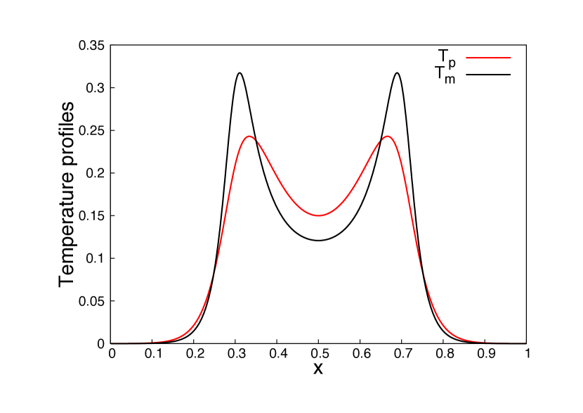
Figure 1: Temperature profiles at $t=0.01s$ for $L=1mm,~{}~{}D_{p}/L^{2}=1s^{-1},~{}~{}c_{p}/C=0.1,~{}~{}c_{m}/C=0.9,~{}~{}v=20m/s,~{}~{}\tau=10^{-3}s$. Initial temperature profiles, $T_{p}=(40/\sqrt{\pi})e^{-(40(x-1/2))^{2}},~{}~{}T_{m}(t=0)=0$.

It is clear that the parameter space of magnetic materials to search for such a behavior is very extended. Here we will discuss just an arbitrary example with model parameters indicated in Fig.1, where we observe such an evolution by numerical integration of (5). We first take as initial phonon temperature profile a narrow Gaussian at the center of the sample. Note, that for these parameters, the discriminant (20) is large and negative, indicative of a strong oscillatory behavior.

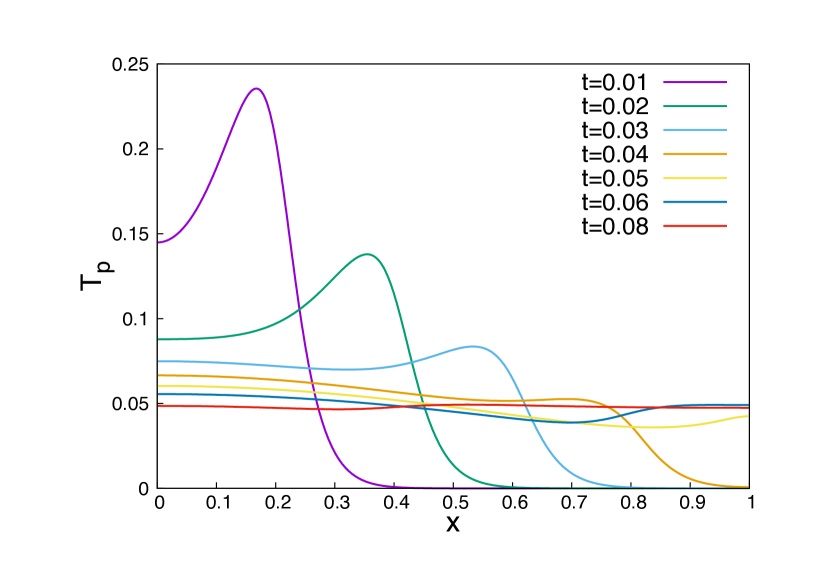
Figure 2: Phonon temperature profiles for the same parameters as in Fig.1. Initial temperature profiles $T_{p}(t=0)=(40/\sqrt{\pi})e^{-(40x)^{2}},~{}~{}T_{m}(t=0)=0$.

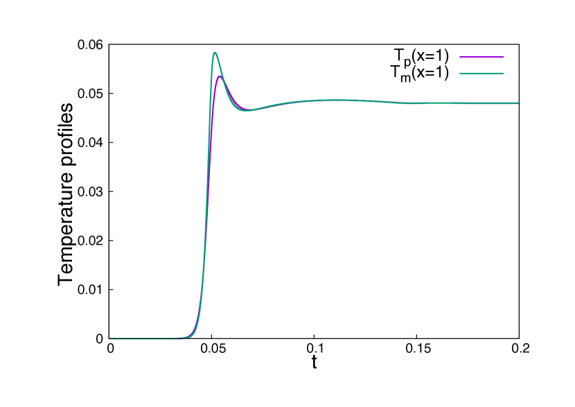
Figure 3: Temperature profiles at $x/L=1$ for the same parameters as in Fig.1. Initial temperature profiles $T_{p}=(40/\sqrt{\pi})e^{-(40x))^{2}},~{}~{}T_{m}(t=0)=0$.

Next, for an initial heat pulse at the left-side of the sample deposited at the phonon subsystem as in a flash experiment, we observe in Fig.2 the propagation of a heat wave, very unlike to a diffusive one, due to the hybridization of the phonon and magnetic components. It results to a characteristic non-monotonic behavior at the right side of the sample as shown in Fig.3. Certainly, further study is required to establish the range of parameters where such a singular temperature evolution can be observed.

In conclusion, to appropriatelly describe the ballistic thermal transport of magnetic excitations coupled to phonons we have introduced a phenomenological advection-diffusion model. This model shows qualitatively different behavior to the SW two-temperature diffusion model. In particular, it implies a greatly enhanced effective diffusion constant for the material parameters of a recent dynamic heat experiment due to the coupled propagation of magnetic and phononic excitations.

Most important, this model predicts a specific two-bump counter-propagating temperature profiles for certain material parameter range. It would by particularly interesting to find materials with appropriate parameters in order to observe such a behavior in a dynamic heat propagation experiment, e.g. direct evidence of ballistic transport by spinons in spin-1/2 Heisenberg chain compounds. Last but not least, althought the proposed model was motivated by the ballistic magnetic transport coupled to the diffusive phonon one in spin chains, it can be applied to any two-component system with coupled advection-diffusion transport.

I Acknowledgments

This work was supported by the Deutsche Forschungsgemeinschaft through Grant HE3439/13. X.Z. acknowledges fruitful discussions with Profs. P. van Loosdrecht and C. Hess on existing and future dynamic heat experiments.

References

(1)
C. Hess, Phys. Rep. 811, 1 (2019).
(2)
N. Hlubek, P. Ribeiro, R. Saint-Martin, A. Revcolevschi, G. Roth,
G. Behr, B. Büchner, C. Hess, Phys. Rev. B81, 020405 (2010).
(3)
X. Zotos, F. Naef and P. Prelovsek,
Physical Review B 55, 11029 (1997).
(4)
W. Parker, R. J. Jenkins, C. P. Butler, and G. L. Abbott,
J. Appl. Phys. 32, 1679 (1961).
(5)
M. Montagnese, M. Otter, X. Zotos, D.A. Fishman, N. Hlubek,
O. Mityashkin, C. Hess, R. Saint-Martin, S. Singh, A. Revcolevschi,
P.H.M. van Loosdrecht, Phys. Rev. Lett. 110, 147206 (2013).
(6)
O.A. Castro-Alvaredo, B. Doyon and T. Yoshimura
Phys. Rev. X6, 041065 (2016);
B. Bertini, M. Collura, J. De Nardis and M. Fagotti,
Phys. Rev. Lett. 117, 207201 (2016).
(7)
D.J. Sanders and D. Walton, Phys. Rev. B 15, 1489 (1977).
(8)
A. V. Sologubenko, K. Giannò, H. R. Ott,
A. Vietkine and A. Revcolevschi, Phys. Rev. B64, 054412 (2001).
(9)
Abramowitz, Milton; Stegun, Irene A., eds. Handbook
of Mathematical Functions with Formulas, Graphs, and Mathematical Tables,
Dover (1965), chap. 22 p. 773.