Gravitationally collapsing stars in $f(R)$ gravity

The gravitational dynamics of a collapsing matter configuration which is simultaneously radiating heat flux is studied in $f(R)$ gravity. Three particular functional forms in $f(R)$ gravity are considered to show that it is possible to envisage boundary conditions such that the end state of the collapse has a weak singularity and that the matter configuration radiates away all of its mass before collapsing to reach the central singularity.

Keywords:  Gravitational collapse. $f(R)$ gravity.

1 Introduction

The general theory of relativity (GR) is an impeccably robust relativistic theory of gravity. It forms the basis for our understanding of gravitational phenomenon at small as well as large scales [1, 2]. However, it is well known that GR cannot be the ultimate theory of gravitation since it has a well defined regime of validity; for example, understanding past and future spacetime singularities are beyond the reach of GR. Suitable modification(s) of GR is(are) essential to understand singularities, or to resolve them. It is believed that a quantum theory of gravity may lead to solution to the problems affecting GR [2, 3, 4, 5, 6]. Naturally, in absence of any consensus on the theory of quantum gravity, modified theories of gravity with quantum corrections are also of interest. The Einstein- Hilbert action may be thought of as only a low energy contribution and higher curvature terms consistent with the diffeomorphism invariance may become relevant as one goes to higher energies. Higher curvature corrections should leave imprints at low energy scales which become important for low energy physics too [5, 6, 7]. Out of these alternate theories, we shall study the $f(R)$ model since it has been found interesting in the cosmological studies as well. These $f(R)$ gravity models are thought of as alternate to the dark energy models [8, 9, 10]. The standard way to construct these $f(R)$ theories is to replace the Einstein- Hilbert Lagrangian by a well defined function of Ricci scalar, $f(R)$ (for general relativity $f(R)=R$) [11]. For a detailed review of the motivation, validity of various functional forms $f(R)$, applications as well as shortcomings of these gravity theories have been extensively analyzed [12, 13, 14, 15, 16, 17, 18, 19, 20].

The purpose of the present work is to construct some examples of spacetimes in $f(R)$ gravity which admit gravitationally weak spacetime singularities [21]. The physical situation which we consider here is the following: the initial mass of the collapsing star or matter configuration is so high that the force of gravity overwhelms the thermal or quantum mechanical pressures. As a result, no stable configuration such as a neutron star or a white dwarf exists during the collapse process. Generically, such collapsing matter configurations admit diverging density and curvatures at the central singularity (we must emphasize that spherically symmetry is assumed throughout the collapse). However, we shall show below that it is possible, without violating energy conditions, that during the gravitational collapse matter is radiated away at such a rate that the matter boundary never reaches its horizon. In this case, no horizon is formed at the boundary since the star radiates off all its mass before reaching the singularity. The central singularity is naked but is gravitationally weak. During this process, all the physical quantities energy density, radial and tangential pressure, pressure anisotropy, heat flux, remain regular and positive throughout the collapse. The luminosity and adiabatic index are also regular and positive, and admits maximum value when the matter approaches the singularity. Thus, for an observer at infinity observing the collapse, the configuration shall become extremely bright, reaching its maximum luminosity before turning off, indicating that it has radiated off all its mass. Solutions of such kind are not unknown and is possible in the Newtonian gravity as well. Consider a star in the Newtonian gravity which is extremely heavy to be supported by the Pauli exclusion principle alone. So, when the gravitation contraction takes place, thermal pressure may balance to some extent. But since there is no event horizon, the star shall continue to radiate all the gravitational energy to infinity. Hence all the matter contained in the star shall be converted to thermal radiation and radiated off. We show here that configurations of similar nature are also possible in $f(R)$ gravity.

From a theoretical point of view, gravitational collapse of matter is important and recently, there has been an increasing interest to understand whether the nature of collapse is altered in modified gravity [18, 22, 23, 24, 25]. Although it remains to study in detail if compact objects formed in theories like the $f(R)$ gravity can be experimentally detected, several investigations have already been carried out in this direction . The idea is to use the multi-wavelength and well as the gravitational wave data to probe matter under extreme gravity (like the composition of the inner core of a neutron star) which remain unknown, as neither they can they be probed directly with astrophysical observations nor are they they within the reach of the present- day theory experiments. Alternatively, the direct gravitational wave data have also made it possible to investigate if these objects are possible in alternate gravity theories. In particular, the recent detection of GW190814, have fueled the speculation that it might be the heaviest neutron star till date [26]. It has been argued that some models of $f(R)$ gravity can indeed explain the origin of such a large mass of $(2.5$-$2.7)M_{\odot}$, even using the well- known equations of state [27, 28].

In this paper, we shall not concern ourselves with compact objects like the white dwarf or a neutron star. We shall assume that the matter is extremely massive, and such objects continue to collapse under its own gravity. The gravitational collapse phenomenon in GR show that the collapse outcome depends upon, among other quantities, the choices of mass profiles and velocity profiles of the collapsing matter. In the context of inhomogeneous LTB models in GR, these issues have been considered in great detail for various matter models including dust and viscous fluids [29]. The stellar collapse of stellar collapse in $f(R)$ gravity using different forms of $f(R)$ function and different matter distributions may be found in [30, 31, 32, 33, 34, 35, 36, 37, 38, 39, 40, 41, 42, 43, 44]. Although different type of $f(R)$ models may be considered, only the ones which are in agreement with the standard cosmological observations should be of interest. Here, we consider three models of $f(R)$ gravity given respectively by: $(a)\leavevmode\nobreak\ f(R)=(R+\lambda R^{2})$ [45]  ,  $(b)\leavevmode\nobreak\ f(R)\sim R^{1+\epsilon}$, with $\epsilon<<1$ [35] and $(c)\leavevmode\nobreak\ f(R)=R+\lambda\,\left[\exp{(-\sigma R)}-1\right]$, with $\lambda\sigma<1$,  [46]. All three theories play a major role in the study of the early and the late universe. For example, in the $R+\lambda R^{2}$ model, the $R^{2}$ term is weak in the weak gravity regime. But it also contributes significantly during the early universe and in strong gravity regime. Here, we study gravitational collapse of an extremely massive object (so massive that its gravitational attraction predominates thermal or quantum mechanical pressures), and so naturally, since we are in a strong gravitational field, this model may assume significance. In all these theories, we shall show that an extremely massive spherical matter cloud, admitting radial and tangential pressures, and outgoing heat flux, can collapse in a manner that no horizon is formed at the boundary (since the star radiates off all its mass before reaching the singularity) making the central singularity naked but weakly singular. To ensure that the gravitational collapse proceeds continuously without forming any stable object, we assume the radius of the $2$- sphere cross- sections decrease linearly with time. The interior collapsing spacetime shall be smoothly matched with the exterior Vaidya spacetime [47] over a timelike surface $\Sigma$ [48].

We approach the problem as follows. In section 2, we give the field equations of $f(R)$ gravity and the junction conditions for smooth matching of the interior and the exterior spacetimes across the timelike hypersurface $\Sigma$. This section also includes the solutions of the $f(R)$ field equations along with the explicit expressions for physical quantities. For the solution, we use the Karmarkar condition [49, 50, 51]. These conditions determine gravitational potentials for static and non- static systems [52, 53, 54, 55]. We must mention here that similar studies on $f(R)$ gravity have been carried out in [39]. However, the solutions obtained there are restrictive in the sense that one of the metric function have been kept constant to derive the values of other metric function. On the other hand we shall show that such conditions are overly restrictive. Note that since Karmarkar condition expresses relationship between metric functions, the forms of metric functions are arbitrary, and dependent on one’s choice. However we argue that this arbitrariness may be removed if metric functions are related to matter variables. For example, if we assume a specific form of pressure anisotropy (difference of the radial and tangential pressures, denoted by $\Delta=p_{t}-p_{r}$), this gives rise to unambiguous set of gravitational potentials, and a class of metric representing collapsing spacetimes. We inspect the physical relevance of these exact solutions by verifying the energy conditions. The stability criteria and discussion about the luminosity and adiabatic index, radial and transverse velocity are carried out in section 2.1. It is shown that a faraway observer will see a source whose luminosity is exponentially increasing until a time when it shuts off quickly. This is due to the fact that the total mass of the star radiates linearly and, as the star reaches its maximum luminosity there is no mass left to radiate. The evolution of the temperature profiles during stellar collapse is also studied in section 2.2 since they play an important role in the study of transport processes in radiative gravitational collapse [56, 57, 58, 59, 60, 61, 62, 63, 64]. In section 3 contains discussion of the results accompanied with concluding remarks.

2 Field Equations and Matching Conditions

The action for the $f(R)$ gravity is obtained by replacing the standard Einstein- Hilbert Lagrangian by a well defined function of Ricci scalar [15]

$$\mathcal{S} = \frac{1}{2}\,\int\sqrt{-g}\,\left[\,f(R)+2\,\mathcal{L}_{M}(g_{\mu\nu},\Psi_{m})\right]d^{4}x\,,$$ (1)

where $\Psi_{m}$ refers collectively to all matter fields, $\mathcal{L}_{M}$ is the Lagrangian density of the matter fields $\Psi_{m}$, $g$ is the determinant of the metric tensor $g_{\mu\nu}$, $R$ is the Ricci scalar curvature and $f(R)$ is the generic function of Ricci scalar defining the theory under consideration and $($using units with $c=1=8\pi G)$. Varying the action (1) with respect to the metric tensor $g_{\mu\nu}$ yields the following field equations:

$$F(R)\,R_{\mu\nu}-\frac{1}{2}f(R)\,g_{\mu\nu}-\left(\nabla_{\mu}\,\nabla_{\nu}-g_{\mu\nu}\,\Box\right)F(R)=T^{M}_{\mu\nu},$$ (2)

where $F(R)={d\,f(R)}/{dR}$,  and $\Box\equiv\nabla_{\mu}\nabla^{\mu}$. This equation may also be rewritten as

$$R_{\mu\nu}-(1/2)\,g_{\mu\nu}\,R=F(R)^{-1}\,\left(T^{M}_{\mu\nu}+T^{D}_{\mu\nu}\right)\,,$$ (3)

where the left side of the equation (3) is the usual Einstein tensor, $T^{M}_{\mu\nu}$ and $T^{D}_{\mu\nu}$ are the energy momentum tensor and effective energy momentum tensor having the form as:

$$T^{M}_{\mu\nu} = (p_{t}+\rho)u_{\mu}u_{\nu}+p_{t}g_{\mu\nu}+(p_{r}-p_{t})X_{\mu}X_{\nu}+q_{\mu}u_{\nu}+q_{\nu}u_{\mu}\,,$$ (4)

$$T^{D}_{\mu\nu} = (1/2)\left[f(R)-R\,F(R)\right]\,g_{\mu\nu}+\left(\nabla_{\mu}\nabla_{\nu}-g_{\mu\nu}\,\Box\right)F(R).$$ (5)

Here, $\rho$, $p_{r}$ and $p_{t}$ are the energy density, radial pressure and the tangential pressure respectively. Also, $q^{\mu}$ $u^{\mu}$, $X^{\mu}$ represents the radial heat flow vector, $4$-velocity vector and spacelike $4$-vector respectively, which satisfy $u_{\mu}u^{\mu}=-X_{\mu}X^{\mu}=-1$ and $u_{\mu}X^{\mu}=u_{\mu}q^{\mu}=0$.

We now consider a general non- static shear free spherically symmetric spacetime metric given by the following form

$$ds^{2}=-a(r)^{2}dt^{2}+b(r)^{2}s(t)^{2}\left(dr^{2}+r^{2}d\theta^{2}+r^{2}\sin^{2}{\theta}d\phi^{2}\right).$$ (6)

The forms of $u^{\mu}$, $X^{\mu}$ and $q^{\mu}$ in terms of the metric (6) are

$$u^{\mu}=a^{-1}\,\delta^{\mu}_{0}\,;\leavevmode\nobreak\ \leavevmode\nobreak\ \leavevmode\nobreak\ \leavevmode\nobreak\ \,\,\,\,X^{\mu}=(b\,s)^{-1}\,\delta^{\mu}_{1}\,\,;\leavevmode\nobreak\ \leavevmode\nobreak\ \leavevmode\nobreak\ \,\,\,\,q^{\mu}=(b\,s)^{-1}\,X^{\mu},$$ (7)

The magnitude of the expansion scalar $\Theta$ and Ricci scalar for the metric (6) have the form

$$\Theta = \bigtriangledown_{\mu}u^{\nu}=\frac{3\,\dot{s}}{a\,s},$$ (8)

$$R = 6\,\frac{s\ddot{s}+\dot{s}^{2}}{a^{2}\,s^{2}}-\frac{2}{b^{2}\,s^{2}}\left[\frac{a^{\prime\prime}}{a}-\frac{b^{\prime 2}}{b^{2}}+\frac{a^{\prime}b^{\prime}}{a\,b}+2\frac{b^{\prime\prime}}{b}+\frac{2}{r}\left(\frac{a^{\prime}}{a}+2\frac{b^{\prime}}{b}\right)\right].$$ (9)

The field equations in $f(R)$ gravity for the metric (6), energy momentum tensor (4), (5) and (7) are

$$\rho=\frac{F}{s^{2}}\left[\frac{3\,\dot{s}^{2}}{a^{2}}-\frac{1}{b^{2}}\left(\frac{2\,b^{\prime\prime}}{b}-\frac{b^{\prime}\,{}^{2}}{b\,^{2}}+\frac{4}{r}\frac{b^{\prime}}{b}\right)\right]+\left(\frac{f-R\,F}{2}\right)+\frac{3\dot{s}\dot{F}}{s\,a^{2}}-\frac{1}{b^{2}\,s^{2}}\left[F^{\prime\prime}+F^{\prime}\left(\frac{b^{\prime}}{b}+\frac{2}{r}\right)\right],$$ (10)

$${p}_{r} = \frac{F}{s^{2}}\left[-\frac{1}{a^{2}}\left(2s\,\ddot{s}+\dot{s}^{2}\right)+\frac{1}{b^{2}}\left(\frac{2\,a^{\prime}\,b^{\prime}}{a\,b}+\frac{2}{r}\left(\frac{a^{\prime}}{a}+\frac{b^{\prime}}{b}\right)+\frac{b^{\prime}\,{}^{2}}{b\,^{2}}\right)\right]-\left(\frac{f-R\,F}{2}\right)$$ (11)

$$\leavevmode\nobreak\ \leavevmode\nobreak\ \leavevmode\nobreak\ \leavevmode\nobreak\ \leavevmode\nobreak\ \leavevmode\nobreak\ \leavevmode\nobreak\ \leavevmode\nobreak\ \leavevmode\nobreak\ \leavevmode\nobreak\ \leavevmode\nobreak\ \leavevmode\nobreak\ \leavevmode\nobreak\ \leavevmode\nobreak\ \leavevmode\nobreak\ \leavevmode\nobreak\ \leavevmode\nobreak\ \leavevmode\nobreak\ \leavevmode\nobreak\ \leavevmode\nobreak\ \leavevmode\nobreak\ \leavevmode\nobreak\ \leavevmode\nobreak\ \leavevmode\nobreak\ \leavevmode\nobreak\ \leavevmode\nobreak\ \leavevmode\nobreak\ \leavevmode\nobreak\ \leavevmode\nobreak\ \leavevmode\nobreak\ \leavevmode\nobreak\ \leavevmode\nobreak\ \leavevmode\nobreak\ \leavevmode\nobreak\ \leavevmode\nobreak\ \leavevmode\nobreak\ -\frac{\dot{F}}{a^{2}}\left(\frac{\ddot{F}}{\dot{F}}+\frac{2\dot{s}}{s}\right)+\frac{F^{\prime}}{b^{2}\,s^{2}}\left(\frac{a^{\prime}}{a}+\frac{2}{r}+\frac{2b^{\prime}}{b}\right),$$

$${p}_{t} = \frac{F}{s^{2}}\left[-\frac{1}{a^{2}}\left(2s\,\ddot{s}+\dot{s}^{2}\right)+\frac{1}{b^{2}}\left(\frac{a^{\prime\prime}}{a}+\frac{b^{\prime\prime}}{b}-\frac{b^{\prime}\,{}^{2}}{b\,^{2}}+\frac{1}{r}\left(\frac{a^{\prime}}{a}+\frac{b^{\prime}}{b}\right)\right)\right]-\left(\frac{f-R\,F}{2}\right)$$ (12)

$$\leavevmode\nobreak\ \leavevmode\nobreak\ \leavevmode\nobreak\ \leavevmode\nobreak\ \leavevmode\nobreak\ \leavevmode\nobreak\ \leavevmode\nobreak\ \leavevmode\nobreak\ \leavevmode\nobreak\ \leavevmode\nobreak\ \leavevmode\nobreak\ \leavevmode\nobreak\ \leavevmode\nobreak\ \leavevmode\nobreak\ \leavevmode\nobreak\ \leavevmode\nobreak\ \leavevmode\nobreak\ \leavevmode\nobreak\ \leavevmode\nobreak\ \leavevmode\nobreak\ \leavevmode\nobreak\ \leavevmode\nobreak\ \leavevmode\nobreak\ \leavevmode\nobreak\ \leavevmode\nobreak\ \leavevmode\nobreak\ \leavevmode\nobreak\ \leavevmode\nobreak\ \leavevmode\nobreak\ \leavevmode\nobreak\ \leavevmode\nobreak\ \leavevmode\nobreak\ \leavevmode\nobreak\ -\frac{\dot{F}}{a^{2}}\left(\frac{\ddot{F}}{\dot{F}}+\frac{2\dot{s}}{s}\right)+\frac{1}{b^{2}\,s^{2}}\left(F^{\prime\prime}+F^{\prime}\left(\frac{a^{\prime}}{a}+\frac{1}{r}\right)\right),$$

$$q=-\frac{2\,a^{\prime}\,\dot{s}\,\dot{F}}{a^{2}\,b^{2}\,s^{3}}+\frac{1}{a^{2}\,b^{2}\,s^{2}}\left(\dot{F}\,^{\prime}-\frac{\dot{F}a^{\prime}}{a}-\frac{\dot{s}\,F^{\prime}}{s}\right),$$ (13)

where prime and dot are the derivatives with respect to $r$ and $t$ respectively.

Let us consider the junction conditions for the smooth matching of the interior manifold $\mathcal{M^{-}}$ (equation (6) considered above) with the exterior manifold $\mathcal{M^{+}}$ across timelike hypersurface $\Sigma$, at $r=r_{b}$. As described in [65, 66], the junction conditions for the $f(R)$ gravity requires the matching of several geometric quantities other than the induced metric ($h_{ij}$) and the extrinsic curvature ($K_{ij})$. In fact, it has been established that in $f(R)$ gravity, the following variables must be matched at the boundary:

$$[h_{ij}]_{-}^{+} = 0,$$ (14)

$$F(R)\,[K_{ij}-(1/3)K\,h_{ij}]_{-}^{+} = 0,$$ (15)

$$\leavevmode\nobreak\ [K]_{-}^{+} = 0,$$ (16)

$$(\partial F(R)/\partial R)\,[\partial_{\tau}R]_{-}^{+} = 0,$$ (17)

$$\leavevmode\nobreak\ [R]_{-}^{+} = 0,$$ (18)

where $\tau$ represents the proper time of the timelike hypersurface, and $K$ is the trace of the extrinsic curvature. Out of these five conditions, for the set of $f(R)$ theories under consideration, it is sufficient to match the metric, the extrinsic curvature, the Ricci scalar, and the derivative of the Ricci as given above, determined from either sides.

The Vaidya spacetime in the outgoing coordinate is taken to be our exterior spacetime $\mathcal{M^{+}}$ [47]

$$ds^{2}_{+}=-\left[1-\frac{2\,M(v)}{{\bf{r}}}\right]\,dv^{2}-2dvd{\bf{r}}+{\bf{r}}^{2}\left(d\theta^{2}+\sin^{2}\theta d\phi^{2}\right),$$ (19)

For our later convenience, let us define the proper time, $d\tau=a(r)_{{}_{\Sigma}}\,dt$. The junction condition as given (14), implies the following conditions

$${\bf{r}}_{{}_{\Sigma}}(v) = (r\,b\,s)_{{}_{\Sigma}},$$ (20)

$$\left(\frac{dv}{d\tau}\right)_{\Sigma}^{-2} = \left(1-\frac{2M}{\bf{r}}+2\frac{d\bf{r}}{dv}\right)_{\Sigma},$$ (21)

where $\tau$ represents the proper time defined on the hypersurface $\Sigma$. The normal vector fields to $\Sigma$ are given by

$$n^{-}_{l}=\left[0,(b\,s)_{{}_{\Sigma}},0,0\right],\leavevmode\nobreak\ \leavevmode\nobreak\ \leavevmode\nobreak\ \leavevmode\nobreak\ \leavevmode\nobreak\ \leavevmode\nobreak\ \leavevmode\nobreak\ n^{+}_{l}=\left[1-\frac{2M}{{\bf{r}}}+2\frac{d{\bf{r}}}{dv}\right]^{-\frac{1}{2}}_{\Sigma}\left[-\frac{d{\bf{r}}}{dv}\delta^{0}_{l}+\delta^{1}_{l}\right]_{\Sigma}.$$ (22)

The extrinsic curvatures for metrics (6) and (19) are given by

$$K^{-}_{\tau\tau} = -\left[\frac{a^{\prime}}{a\,b\,s}\right]_{\Sigma},K^{-}_{\theta\theta}=\left[r\,b\,s\left(1+\frac{r\,b^{\prime}}{b}\right)\right]_{\Sigma},$$ (23)

$$K^{+}_{\tau\tau} = \left[\frac{d^{2}v}{d\tau^{2}}\left(\frac{dv}{d\tau}\right)^{-1}-\left(\frac{dv}{d\tau}\right)\frac{M}{{\bf{r}}^{2}}\right]_{\Sigma},K^{+}_{\theta\theta}=\left[\left(\frac{dv}{d\tau}\right)\left(1-\frac{2M}{{\bf{r}}}\right){\bf{r}}-{\bf{r}}\frac{d{\bf{r}}}{d\tau}\right]_{\Sigma},$$ (24)

$$K^{-}_{\phi\phi} = \sin^{2}{\theta}K^{-}_{\theta\theta}\,\,,\,\,K^{+}_{\phi\phi}=\sin^{2}{\theta}K^{+}_{\theta\theta}.$$ (25)

Now, from the junction condition on $K_{ij}$ (because of the conditions that $K$ must satisfy on the hypersurface, matching $K_{ij}$ is enough), we get the following. From the equality for the $\theta\theta$ components at hypersurface $\Sigma$, and the equations (20) and (21), we obtain

$$\left[r\,b\,s\left(1+\frac{r\,b^{\prime}}{b}\right)\right]_{\Sigma} = \left[\left(\frac{dv}{d\tau}\right)\left(1-\frac{2M}{{\bf{r}}}\right){\bf{r}}-{\bf{r}}\frac{d{\bf{r}}}{d\tau}\right]_{\Sigma},$$ (26)

and the total energy inside the boundary hypersurface $\Sigma$, given by the Misner- Sharp mass, denoted by $2m$ (such that $m=M$ on the matching hypersurface) [67, 68], where

$$m_{\Sigma} = \left[\frac{r^{3}\,\dot{s}^{2}\,b^{3}s}{2\,a^{2}}-\frac{r^{3}\,s\,b^{\prime}\,{}^{2}}{2\,b}-r^{2}\,s\,b^{\prime}\right]_{\Sigma}.$$ (27)

Now, again from the matching of the $K^{+}_{\tau\tau}=K^{-}_{\tau\tau}$ component we have the following equation:

$$-\left[\frac{a^{\prime}}{a\,b\,s}\right]_{\Sigma} = \left[\frac{d^{2}v}{d\tau^{2}}\left(\frac{dv}{d\tau}\right)^{-1}-\left(\frac{dv}{d\tau}\right)\frac{M}{{\bf{r}}^{2}}\right]_{\Sigma},$$ (28)

and, substituting the relation between proper and coordinate time along with the eqns. (20) and (27) into the eqn.(26) we have

$$\left(\frac{dv}{d\tau}\right)_{\Sigma} = \left(1+\frac{r\,b^{\prime}}{b}+\frac{r\,b\,\dot{s}}{a}\right)_{\Sigma}^{-1}.$$ (29)

Now, differentiating (29) with respect to the $\tau$ and using eqns (27) and (29), we can rewrite (28). Further, comparing with equations (11) and (13) we have the following useful form

$$\left(p_{r}+T^{D}_{rr}+b\,sT^{D}_{tr}\right)_{{}_{\Sigma}} = (q\,b\,s)_{{}_{\Sigma}}.$$ (30)

where,

$$T^{D}_{rr} = \left(\frac{f-R\,F}{2}\right)+\frac{\dot{F}}{a^{2}}\left(\frac{\ddot{F}}{\dot{F}}+\frac{2\dot{s}}{s}\right)-\frac{F^{\prime}}{b^{2}\,s^{2}}\left(\frac{a^{\prime}}{a}+\frac{2}{r}+\frac{2b^{\prime}}{b}\right),$$ (31)

$$T^{D}_{tr} = \frac{1}{a^{2}\,b^{2}\,s^{2}}\left(\dot{F}\,^{\prime}-\frac{\dot{F}a^{\prime}}{a}-\frac{\dot{s}\,F^{\prime}}{s}\right),$$ (32)

are the dark source terms. From equation (30), it is found that just like for general relativity, the radial pressure does not vanish at the boundary but, instead is proportional to the dissipative as well as radiative dark source terms. The extra terms $T^{D}_{rr}$ and $T^{D}_{tr}$ on the LHS of equation (30) are the dark source term and may appear due to the higher order curvature geometry of the collapsing sphere [39].

Let us now move to match $K$ as given in (14). The expressions for the trace of extrinsic curvatures on the either sides lead to the following matching condition on the hypersurface:

$$\left[p_{r}+T^{D}_{rr}+b\,sT^{D}_{tr}-q\,b\,s\right]_{{}_{\Sigma}}=2\,[M-m]_{{}_{\Sigma}},$$ (33)

and naturally, this condition is identically satisfied due to the abovementioned equations. The matching of the Ricci and its proper time derivative gives the following conditions which are to be satisfied for the metric of the internal manifold (at the hypersurface $\Sigma$):

$$s\ddot{s}+\dot{s}^{2} = \frac{a^{2}}{3b^{2}}\left[\frac{a^{\prime\prime}}{a}+2\frac{b^{\prime\prime}}{b}+\frac{a^{\prime}b^{\prime}}{a\,b}+\frac{2}{r}\left(\frac{a^{\prime}}{a}+2\frac{b^{\prime}}{b}\right)-\frac{b^{\prime 2}}{b^{2}}\right],$$

$$3\dot{s}\ddot{s}+s\dddot{s} = 0.$$ (34)

The metric of the internal manifold must be chosen so as to satisfy the two conditions in (2). To determine metric functions according to all these junction conditions, it is necessary to use some auxiliary conditions. We shall see below that these equations are consistent with a collapsing time dependent internal metric. In fact, one may argue that junction conditions indeed force such a possibility. Additionally, we must also ascertain the physical viability of the spacetime metric. From equations (11), (12) and (6), the pressure anisotropy factor $\Delta=p_{t}-p_{r}$ has the form

$$\Delta = \frac{F}{b^{2}\,s^{2}}\left[\frac{b^{\prime\prime}}{b}-\frac{2\,b^{\prime\,^{2}}}{b^{2}}+\frac{a^{\prime\prime}}{a}-\frac{2\,a^{\prime}\,b^{\prime}}{a\,b}-\frac{1}{r}\left(\frac{a^{\prime}}{a}+\frac{b^{\prime}}{b}\right)\right]+\frac{F^{\prime\prime}}{b^{2}\,s^{2}}-\frac{F^{\prime}}{b^{2}\,s^{2}}\left(\frac{2b^{\prime}}{b}+\frac{1}{r}\right).$$ (35)

The general expression for the shear free spacetime as given in (35) is has the complicated form. To find the solution of the metric functions and mathematical simplicity, we take an adhoc form of the pressure anisotropy $\Delta$ to be:

$$\Delta = \frac{F^{\prime\prime}}{b^{2}\,s^{2}}-\frac{F^{\prime}}{b^{2}\,s^{2}}\left(\frac{2b^{\prime}}{b}+\frac{1}{r}\right)-\frac{F}{b^{2}\,s^{2}}\left[\frac{2\,a^{\prime}\,b^{\prime}}{a\,b}-\frac{a^{\prime\prime}}{a}+\frac{a^{\prime}}{r\,a}\right]$$ (36)

Although, we have chosen this form of the anisotropy in pressure $\Delta$ for the mathematical simplicity, later we will see that they represents the physically viable solutions of the potentials. Also, this choice of $\Delta$ is physically significant, such that $\Delta$ is regular throughout the collapse. It must be noted that this choice of the anisotropy $\eqref{Delta1}$ reduces the total pressure anisotropic equation (35) as differential equation of only one function, given by

$$0 = \frac{1}{s^{2}\,b^{2}}\left(\frac{b^{\prime\prime}}{b}-\frac{2\,b^{\prime\,^{2}}}{b^{2}}-\frac{b^{\prime}}{r\,b}\right),$$ (37)

The form of the function $b(r)$ is

$$b(r) = -2[C_{3}\,r^{2}+2\,C_{4}]^{-1},$$ (38)

where $C_{3}$ and $C_{4}$ are constant of integration.

Let us now use the fact that under certain conditions, a $(n+1)$-dimensional space can be embedded into a pseudo Euclidean space of dimension $(n+2)$ [49]. Thus the necessary and sufficient condition for any Riemannian space to be an embedding class $\bf{I}$ is the Karmarkar condition [50, 51],

$$R_{rtrt}\,R_{\theta\phi\theta\phi}=R_{r\theta r\theta}\,R_{t\phi t\phi}-R_{\theta rt\theta}\,R_{\phi rt\phi}.$$ (39)

The non vanishing components of the Riemann tensor for the metric (6) are

$$R_{rtrt} = a^{2}\left(\frac{a^{\prime\prime}}{a}-\frac{b^{2}s}{a^{2}}\ddot{s}-\frac{a^{\prime}}{a}\frac{b^{\prime}}{b}\right)\,,\,\,\,R_{\theta\phi\theta\phi}={r^{4}b^{2}s^{2}}\left(\frac{b^{2}}{a^{2}}\dot{s}^{2}-\frac{2b^{\prime}}{rb}-\frac{b^{\prime\,^{2}}}{b^{2}}\right)\sin^{2}\theta,$$ (40)

$$R_{r\theta r\theta} = {r^{2}b^{2}s^{2}}\left(\frac{b^{2}}{a^{2}}\dot{s}^{2}-\frac{b^{\prime}}{rb}-\frac{b^{\prime\prime}}{b}+\frac{b^{\prime\,^{2}}}{b^{2}}\right)\,,\,\,\,R_{\theta rt\theta}=\frac{r^{2}b^{2}s}{a}a^{\prime}\dot{s},$$ (41)

$$R_{t\phi t\phi} = {r^{2}a^{2}b}\left(\frac{a^{\prime}}{ra}-\frac{b^{2}s}{a^{2}}\ddot{s}+\frac{a^{\prime}}{a}\frac{b^{\prime}}{b}\right)\sin^{2}\theta\,,\,\,\,R_{\phi rt\phi}=\sin^{2}\theta R_{\theta rt\theta}.$$ (42)

Using the expressions for Riemannian tensors from eqns (40)- (42) into the eqn (39) we have

$$0 = b^{2}{\dot{s}}^{2}b^{3}\left(\frac{a^{\prime\prime}}{a}-2\frac{a^{\prime}}{a}\frac{b\prime}{b}+\frac{a^{\prime\,^{2}}}{a^{2}}-\frac{a^{\prime}}{ra}\right)-r^{2}b^{3}s\ddot{s}\left(\frac{b^{\prime\prime}}{b}-2\frac{b^{\prime\,^{2}}}{b^{2}}-\frac{b^{\prime}}{rb}\right)$$ (43)

$$+ r^{2}aa^{\prime}b^{\prime\prime}\left(\frac{b^{\prime}}{b}+\frac{1}{r}\right)-r^{2}aba^{\prime\prime}\left(\frac{b^{\prime\,^{2}}}{b^{2}}+2\frac{b^{\prime}}{rb}\right)+raba^{\prime}\left(\frac{b^{\prime}}{rb}+2\frac{b^{\prime\,^{2}}}{b^{2}}\right).$$

For a given form of metric function $b(r)$ (38), the class I condition in equation (43) is nonlinear. A physical relevant collapsing model must satisfy (30) and (43) simultaneously. It must be noted that simplest choice of solutions of (30) is a linear solution  [69]

$$s(t) = -C_{Z}\,t,$$ (44)

$C_{Z}>0$. The form of the other metric function $a(r)$ is obtained by using equation (38) and (44) into the class $1$ condition (43)

$$a(r) = \frac{1}{2\sqrt{2C_{3}C_{4}}}[C_{4}^{2}\left(C_{1}b(r)+4C_{2}C_{3}\right)^{2}-4C_{Z}^{2}]^{1/2}$$ (45)

where $C_{1}$ and $C_{2}$ are integration constants. Surprisingly, the quantity in the numerator inside the square root, arises naturally from the matching of the Ricci scalar (and it’s derivative), given in (2) These forms of the solutions of the gravitational potentials are same as obtained in [55] for shear free spacetime. In [55], it has been shown that for the static case, Karmarkar condition together with the pressure isotropy yields the Schwarzschild [70] like form of the metric functions. Also, it has been shown that these set of gravitational potentials are the special class of those found in [71]. Thus, although we have assume this particular form of $\Delta$ (36) for the mathematical simplicity, represents the physically viable solutions.

It is now instructive to rewrite the physical quantities of the matter cloud in terms of the metric variables for a better understanding of the dynamics of spacetime during the collapse process. These expressions have been written in detail in the Appendix. The boundary condition (30) in the view of these equations in the Appendix, (63)-(65) becomes

$$2s\,\ddot{s}+\dot{s}^{2}-2x\dot{s}+b\,s\,T^{D}_{rt} = y-T^{D}_{rr},$$ (46)

where $T^{D}_{rr}$ and $T^{D}_{rt}$ are given by equations (31) and (32) respectively and the quantities $x$ and $y$ are

$$x=\left(\frac{a^{\prime}}{b}\right)_{\Sigma},\leavevmode\nobreak\ \leavevmode\nobreak\ \leavevmode\nobreak\ \leavevmode\nobreak\ y=\left(\frac{a^{2}}{b^{2}}\left[\frac{b^{\prime\,^{2}}}{b^{2}}+\frac{2}{r}\frac{b^{\prime}}{b}+\frac{2a^{\prime}b^{\prime}}{ab}+\frac{2}{r}\frac{a^{\prime}}{a}\right]\right)_{\Sigma}.$$ (47)

The metric functions $a(r)$ and $b(r)$ should not vanish during the collapsing phenomena, since otherwise the metric shall become degenerate. This also implies that their signatures remain unchanged. For second metric potential to be positive i.e. $a(r)>0$ we must have, from (45), that

$$C_{Z}^{2}<C_{4}^{2}\left[\frac{C_{1}}{C_{3}r^{2}+2C_{4}}-2C_{2}C_{3}\right]^{2}.$$ (48)

This equation also implies that at the center of the cloud, $r=0$, we must have $C_{Z}<C_{1}-2C_{2}C_{3}C_{4}$.

The graphical representations of the physical quantities (62)-(65) shows that they are well defined throughout the stellar collapse for both the $f(R)$ models. Figs. 1(a) , 1(b) & 1(c) , 2(a) , 2(b) & 2(c) , 3(a) , 3(b) & 3(c) , 4(a) , 4(b) & 4(c) shows that the density, radial pressure, tangential pressure and pressure anisotropy are positive and regular throughout the collapse for all the $f(R)$ models and the parameters considered here. Also, as seen from the Figs. 5(a) , 5(b) & 5(c) , the heat flux increase as the collapse starts and remains positive throughout the collapse for these cases.

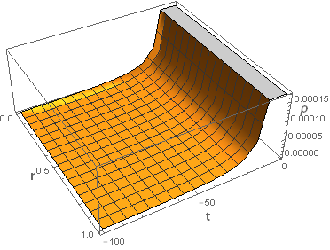
(a)

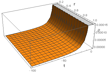
(b)

(c)

Figure 1: (a), (b) & (c) shows the plots of the density $\rho$ (62) w.r.t. time $t$ and radial $r$ coordinates for $f(R)=R+\lambda R^{2}$ with $\lambda=5$, $f(R)=R^{1+\epsilon}$ with $\epsilon=0.01$ and $f(R)=R+\lambda\left[\exp\left(-\gamma R\right)-1\right]$ with $\lambda=0.1$ & $\gamma=0.0002$ respectively. For each of these $f(R)$ models, it remains regular as well as positive throughout the collapse.

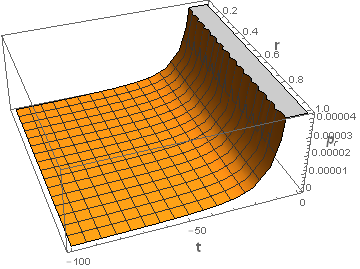
(a)

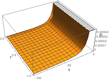
(b)

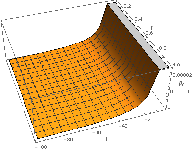
(c)

Figure 2: (a), (b) & (c) shows the plots of the radial pressure $p_{r}$ (63) w.r.t. time $t$ and radial $r$ coordinates for $f(R)=R+\lambda R^{2}$ with $\lambda=5$, $f(R)=R^{1+\epsilon}$ with $\epsilon=0.01$ and $f(R)=R+\lambda\left[\exp\left(-\gamma R\right)-1\right]$ with $\lambda=0.1$ & $\gamma=0.0002$ respectively. For each of these $f(R)$ models, it remains regular as well as positive throughout the collapse.

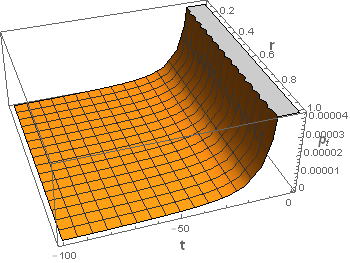
(a)

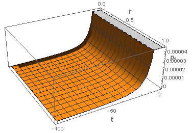
(b)

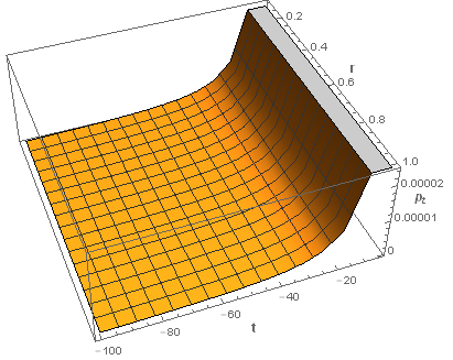
(c)

Figure 3: (a), (b) & (c) shows the plots of the tangential pressure $p_{t}$ (64) w.r.t. time $t$ and radial $r$ coordinates for $f(R)=R+\lambda R^{2}$ with $\lambda=5$, $f(R)=R^{1+\epsilon}$ with $\epsilon=0.01$ and $f(R)=R+\lambda\left[\exp\left(-\gamma R\right)-1\right]$ with $\lambda=0.1$ & $\gamma=0.0002$ respectively. For each of these $f(R)$ models, it remains regular as well as positive throughout the collapse.

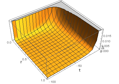
(a)

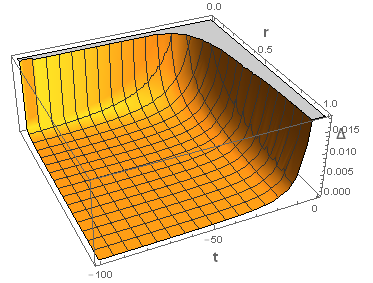
(b)

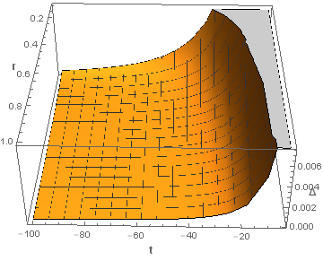
(c)

Figure 4: (a), (b) & (c) shows the plots of the pressure anisotropy $\Delta$ (36) w.r.t. time $t$ and radial $r$ coordinates for $f(R)=R+\lambda R^{2}$ with $\lambda=5$, $f(R)=R^{1+\epsilon}$ with $\epsilon=0.01$ and $f(R)=R+\lambda\left[\exp\left(-\gamma R\right)-1\right]$ with $\lambda=0.1$ & $\gamma=0.0002$ respectively. For each of these $f(R)$ models, it remains regular as well as positive throughout the collapse.

(a)

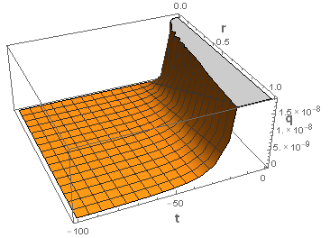
(b)

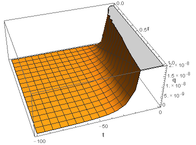
(c)

Figure 5: (a), (b) & (c) shows the plots of the heat flux $q$ (65) w.r.t. time $t$ and radial $r$ coordinates for $f(R)=R+\lambda R^{2}$ with $\lambda=5$, $f(R)=R^{1+\epsilon}$ with $\epsilon=0.01$ and $f(R)=R+\lambda\left[\exp\left(-\gamma R\right)-1\right]$ with $\lambda=0.1$ & $\gamma=0.0002$ respectively. For each of these $f(R)$ models, it remains positive throughout the collapse.

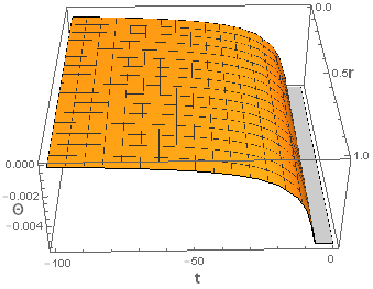
(a)

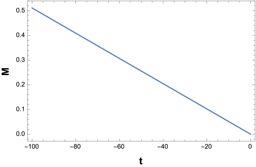
(b)

Figure 6: (a) Plot of the expansion scalar $\Theta$ (66) w.r.t. time $t$ and radial $r$ coordinates. At the beginning of collapse $\Theta$ has zero value and it starts decreasing and remains negative throughout the collapse. (b) Plot of the mass of the collapsing star (67) w.r.t. time $t$, and it shows that mass radiates linearly.

A related quantity of importance in this study is the total luminosity visible to an observer at infinity, which may be defined in terms of the mass loss from the boundary surface:

$$L_{\infty} = -\left(\frac{dm}{dv}\right)_{\Sigma}=\left[\frac{r^{2}\,s^{2}\,b^{2}\,p_{r}}{2}\left(1+\frac{r\,b^{\prime}}{b}+\frac{r\,b\,\dot{s}}{a}\right)^{2}\right]_{\Sigma},$$ (49)

where we have used the equations (11), (27) and (28). Now, as soon as the black hole is formed, by definition, the luminosity of the surface is zero. From the above equation, this implies that sufficient condition for the formation of a black hole is

$$\left[1+\frac{r\,b^{\prime}}{b}+\frac{r\,b\,\dot{s}}{a}\right]_{\Sigma}=0.$$ (50)

Naturally, for any static observer at asymptotic infinity, the redshift diverges at the time of formation of the black hole.

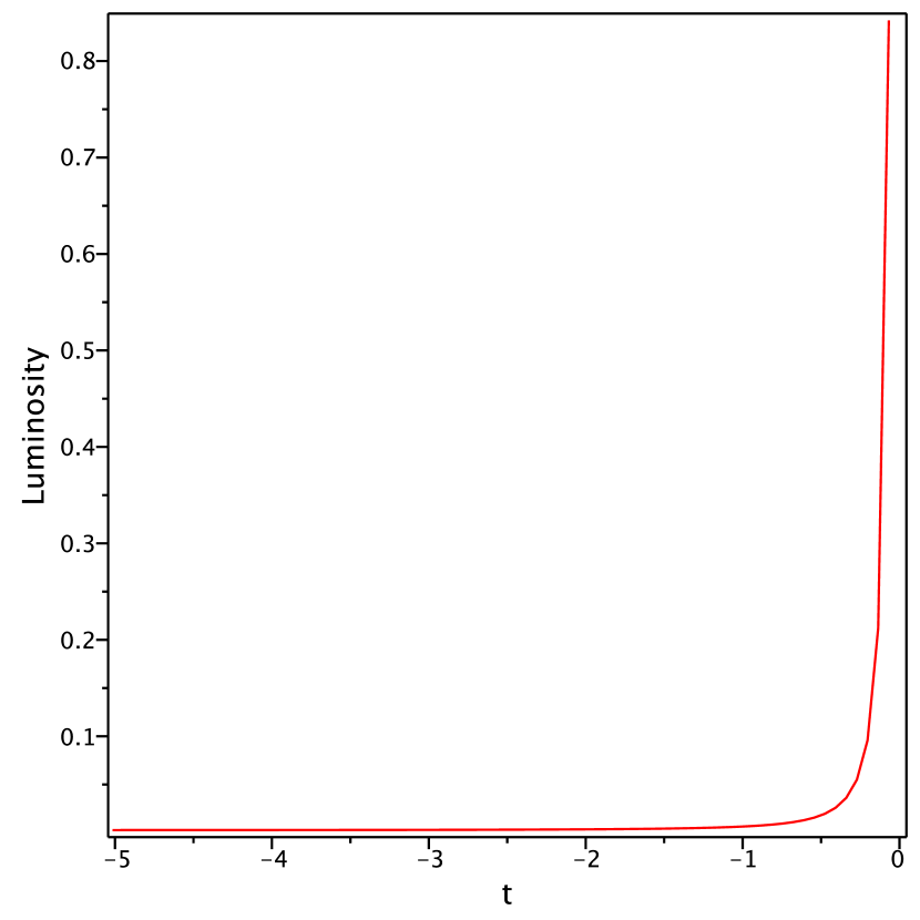
(a)

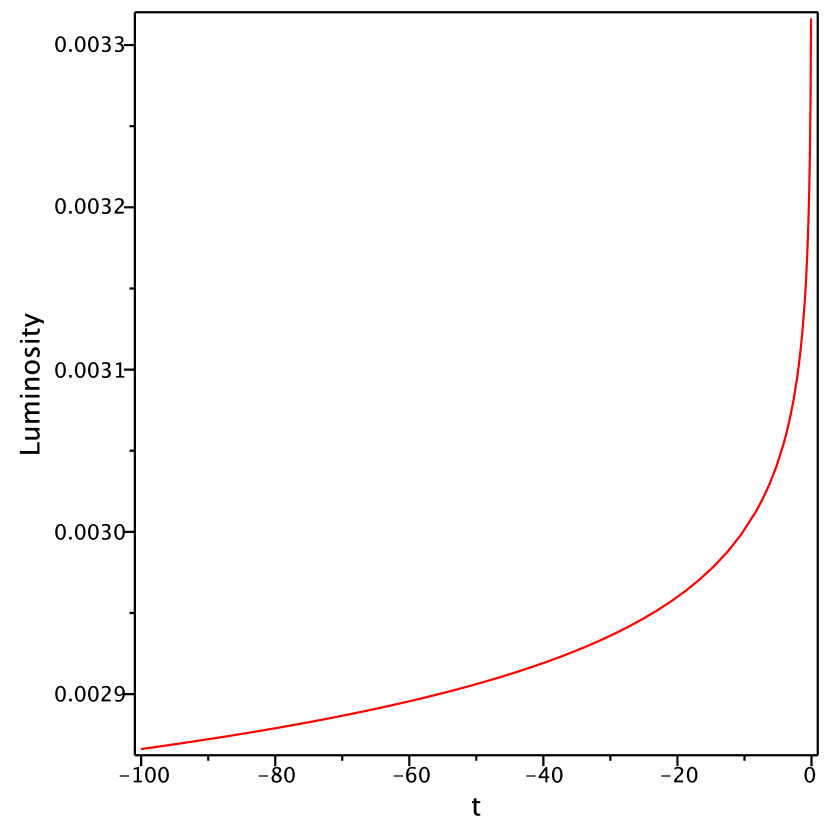
(b)

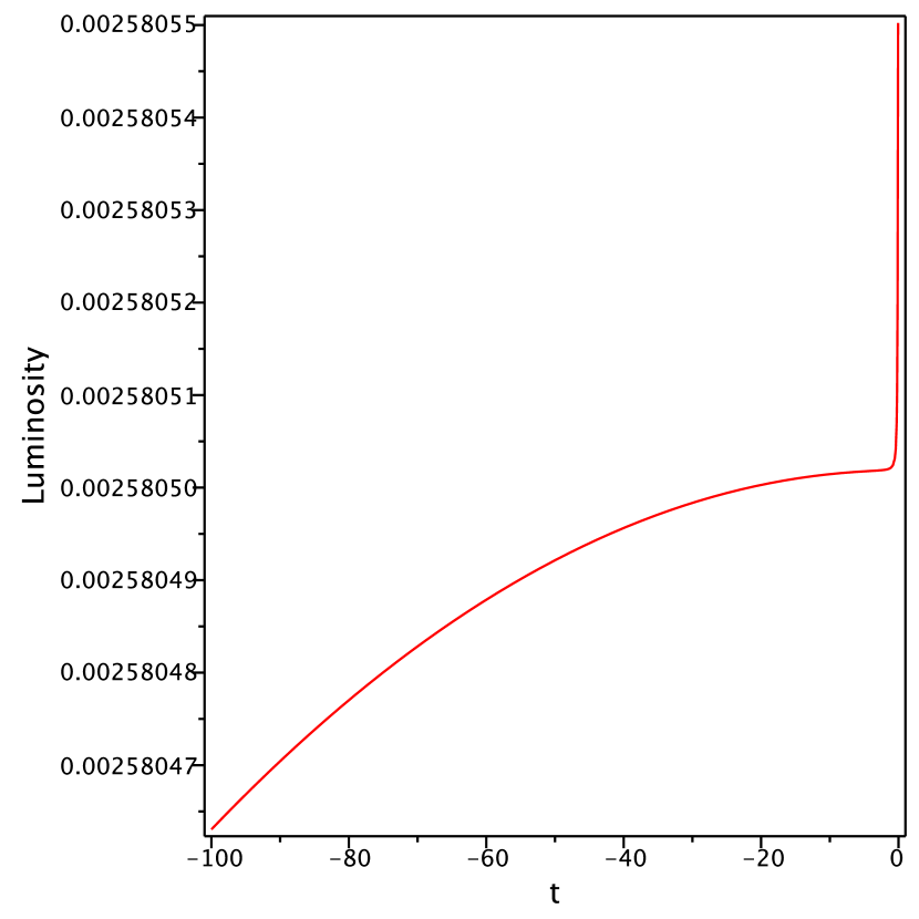
(c)

Figure 7: (a), (b) & (c) shows the plots of the luminosity (49) at $r=r_{\Sigma}=1$, w.r.t. time $t$ for $f(R)=R+\lambda R^{2}$ with $\lambda=5$, $f(R)=R^{1+\epsilon}$ with $\epsilon=0.01$ and $f(R)=R+\lambda\left[\exp\left(-\gamma R\right)-1\right]$ with $\lambda=0.1$ & $\gamma=0.0002$ respectively.

To show that these spacetime solutions are physically viable, we show that they satisfy the energy conditions as well. Indeed, all the energy conditions namely weak (W), null (N), dominant (D) and strong (S) hold good for the collapsing star. In the following we list these conditions [70, 72]
E1 :  $\left(\rho+p_{r}\right)^{2}-4q^{2}\,\geq\,0$                            (D/S/W)
E2 :  $\rho-p_{r}\,\geq\,0\,\,\,\,$                                      (D)
E3 :  $\rho-p_{r}-2p_{t}+\sqrt{\left(\rho+p_{r}\right)^{2}-4q^{2}}\,\geq\,0$   (D)
E4 :  $\rho-p_{r}+\sqrt{\left(\rho+p_{r}\right)^{2}-4q^{2}}\,\geq\,0\,\,\,\,$         (W/D)
E5 :  $\rho-p_{r}+2p_{t}+\sqrt{\left(\rho+p_{r}\right)^{2}-4q^{2}}\,\geq\,0$   (D/W/S)
E6 :  $2p_{t}+\sqrt{\left(\rho+p_{r}\right)^{2}-4q^{2}}\,\geq\,0$                (S)
The star should also satisfy
E7 :  $\rho>0$,  $p_{r}>0$,  $p_{t}>0$, and $\rho^{\prime}<0$,  $p_{r}^{\prime}<0$,  $p_{t}^{\prime}<0$.
It is clear from the above conditions that E1,  E2, E3 & E7 are enough to validate the physical conditions existing inside the star. For the radiating- collapsing stellar models in $f(R)$ gravity, Figs. 8(a), 8(b) & 8(c) show that the energy conditions are positive and regular throughout the interior of the star.

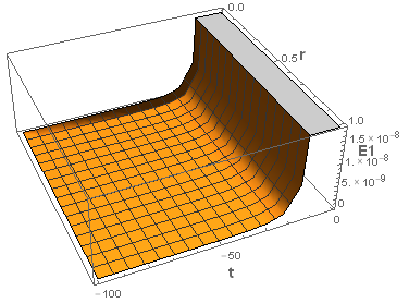
(a)

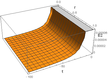
(b)

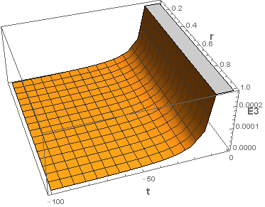
(c)

Figure 8: (a), (b) and (c) shows the plots of energy conditions $E1$, $E2$ and $E3$ w.r.t. time $t$ and radial $r$ coordinates for $f(R)=R+\lambda R^{2}$ with $\lambda=5$ respectively.

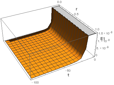
(a)

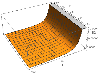
(b)

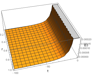
(c)

Figure 9: (a), (b) and (c) shows the plots of energy conditions $E1$, $E2$ and $E3$ w.r.t. time $t$ and radial $r$ coordinates for $f(R)=R^{1+\epsilon}$ with $\epsilon=0.01$ respectively.

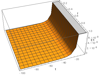
(a)

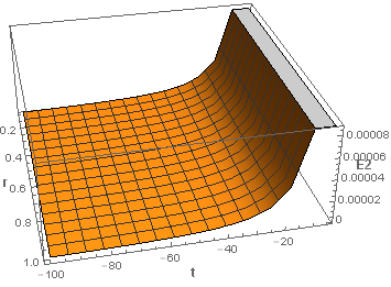
(b)

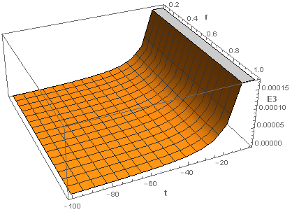
(c)

Figure 10: (a), (b) & (c) shows the plots of energy conditions $E1$, $E2$ and $E3$ w.r.t. time $t$ and radial $r$ coordinates for $f(R)=R+\lambda\left[\exp\left(-\gamma R\right)-1\right]$ with $\lambda=0.1$ & $\gamma=0.0002$ respectively.

2.1 Stability Criteria

The study of dynamical instability (stability) of spherical stellar system shows that for adiabatic index $\Gamma<4/3$ $\left(\Gamma>4/3\right)$ the stellar system becomes unstable (stable) as the weight of the stellar system increase much faster (remains less than) than that of its pressure [73]. Also, the causality condition imposes certain constraints on the dynamics of the stellar system such that inside the star, the radial $V_{r}$ and the transverse $V_{t}$ components of the speed of sound should be less than the speed of the light ($c=1$), so that $0\leq V_{r}\leq 1$ and $0\leq V_{t}\leq 1$ [74]. Thus, to check the stability/instability of the collapsing stellar system, we need to study the behavior of the important physical quantities, adiabatic index, sound of the speed which are defined as [48, 74, 75]

$$\Gamma_{eff} = \left[\frac{\partial(\ln p_{r})}{\partial(\ln\rho)}\right]_{\Sigma}=\left[\left(\frac{\dot{p}_{r}}{p_{r}}\right)\left(\frac{\dot{\rho}}{\rho}\right)\right]_{\Sigma}$$ (51)

$$Vr = \frac{d\,p_{r}}{d\rho}\,\,,\hskip 28.45274ptVt=\frac{d\,p_{t}}{d\rho}$$ (52)

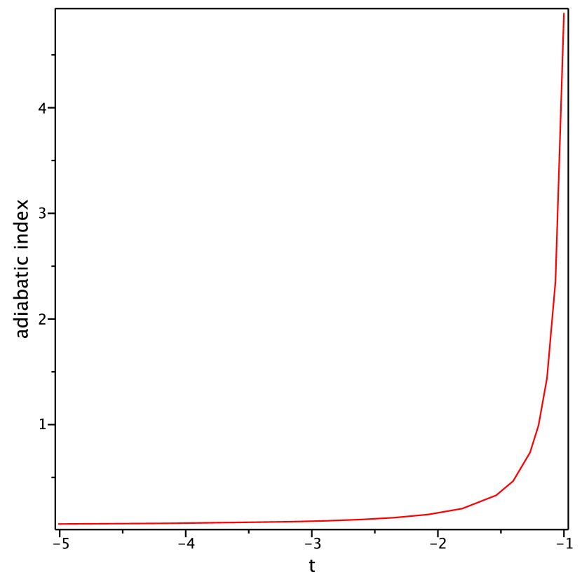
(a)

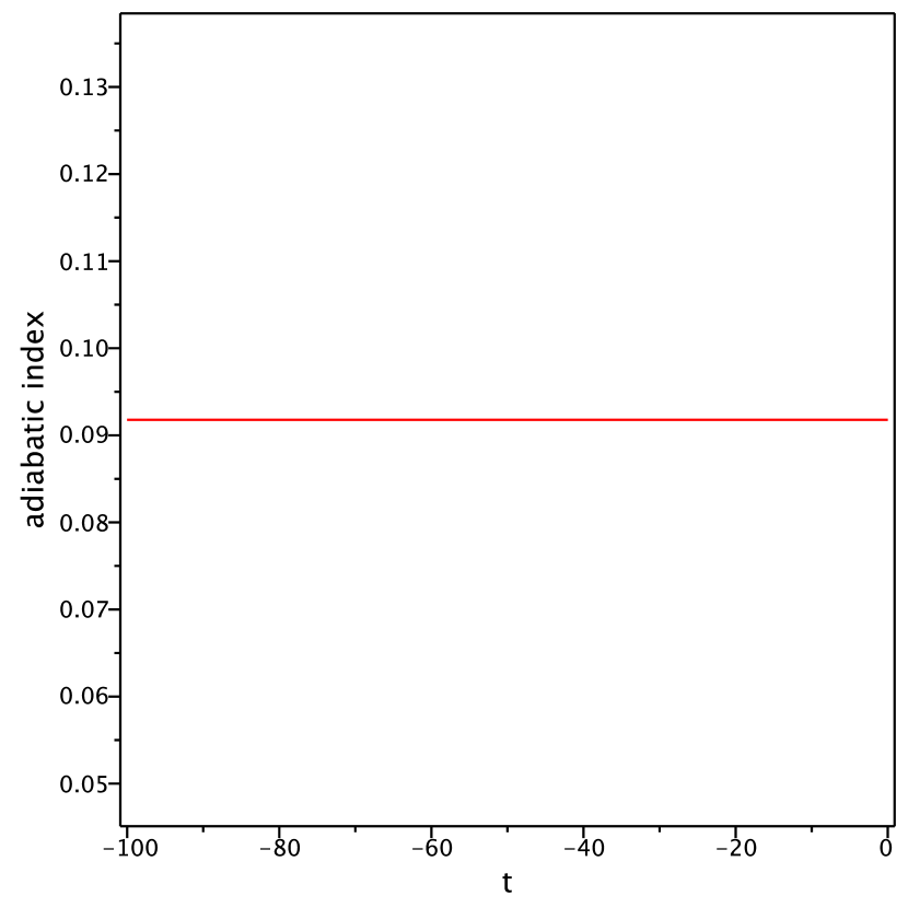
(b)

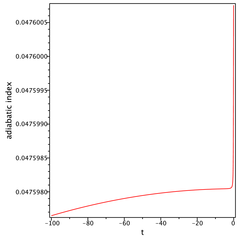
(c)

Figure 11: (a), (b) & (c) shows the plots of adiabatic index at $r=r_{\Sigma}=1$, w.r.t. time $t$ for $f(R)=R+\lambda R^{2}$ with $\lambda=5$, $f(R)=R^{1+\epsilon}$ with $\epsilon=0.01$ and $f(R)=R+\lambda\left[\exp\left(-\gamma R\right)-1\right]$ with $\lambda=0.1$ & $\gamma=0.0002$ respectively

Although stability may be understood from the behavior of the pressure and density variables, the quantities in (51) and (52) are considered to be better to establish stability. For $f(R)=R+\lambda R^{2}$ model with $\lambda=5$, Figs. 7(a) and 11(a) shows that the total luminosity and the adiabatic index are positive and increasing. Note that the adiabatic index attains a maximum value where the luminosity is maximum. This behavior of the luminosity and adiabatic index can be interpreted as follows. Any static observer at asymptotic infinity will see an exponentially radiating radial source until a time when luminosity reaches its maximum value after which it instantaneously turn off. This is due to the fact that the total mass of the star radiates linearly as seen from the Fig. 6(b) and when the star reaches its maximum luminosity, there is no mass left to radiates and hence the observer at rest at infinity will see sudden turn off of the light source. The similar kind of behavior were obtained in [75]. Fig. 11(a) shows that the effective adiabatic index is positive and less than $4/3$ which implies that the considered stellar system is unstable and representing the collapsing scenario [73]. For $f(R)=R^{1+\epsilon}$, and $f(R)=R+\lambda\,\left[\exp{(-\sigma R)}-1\right]$ models, similar behavior of luminosity is obtained as that of for the first model. Fig. 11(b) shows that the effective adiabatic index is constant function of time, and is positive and less than $4/3$, which implies it represents the collapsing scenario. As we have shown graphically that the star radiates all its mass before reaching at the singularity. So, there are no trapped surfaces formed during the collapse. Which implies that neither the black hole nor naked singularity are the end state of the collapse.

2.2 Thermal Properties

Earlier studies have shown that relaxation effects are important to understand dissipative gravitational collapse [57, 58, 59, 62, 76]. To study the temperature profiles, we consider the transport equation for the metric (6) given by [56, 57, 77]

$$\tau h_{\mu}^{\nu}\dot{q}_{\nu}+q_{\mu} = -k\left(h_{\mu}^{\nu}\nabla_{\nu}T+T\dot{u}_{\mu}\right)$$ (53)

$$\tau\left(qbs\right)_{,t}+q\,a\,b\,s = -\frac{k\left(aT\right)_{,r}}{bs},$$ (54)

where, $\alpha>0$, $\beta>0$,  $\gamma>0$ and $\sigma>0$, & $h^{\mu\nu}=g^{\mu\nu}+u^{\mu}u^{\nu}$. Also,

$$\tau_{c}=\left({\alpha/\gamma}\right)\,(T)^{-\sigma}\hskip 5.69046pt,\hskip 17.07182ptk=\gamma\,\tau_{c}\,T^{3}\hskip 5.69046pt,\hskip 17.07182pt\tau=\tau_{c}\,(\beta\,\gamma)/\alpha$$ (55)

where $\tau_{c}$ is the mean collision time, $k$ is thermal conductivity and $\tau$ represents the relaxation time respectively [57][64]. The quantity $\tau$ measures the strength of relaxational effects and is called the causality index. The values $\tau=0$ or $\beta=0$ represents the noncausal temperature profile.

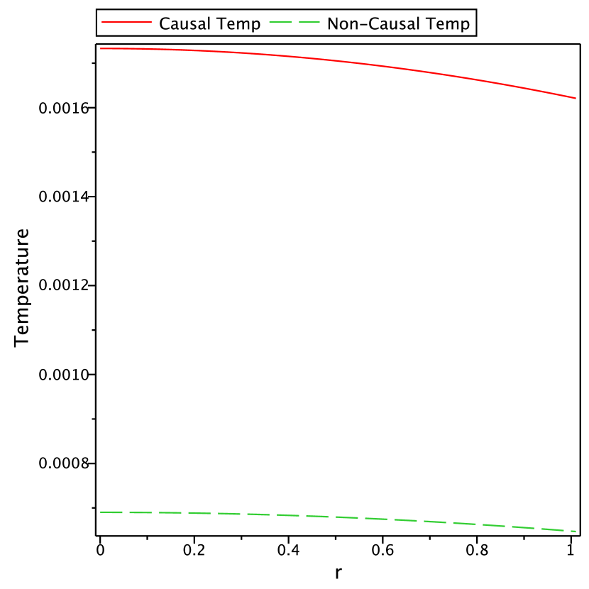
(a)

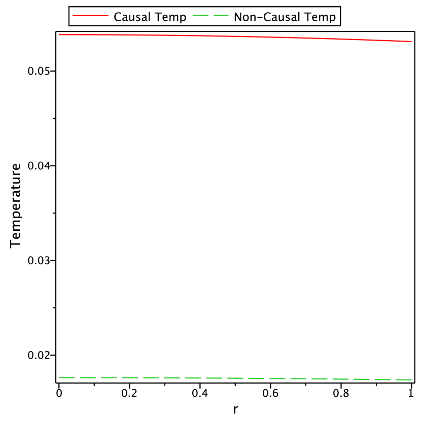
(b)

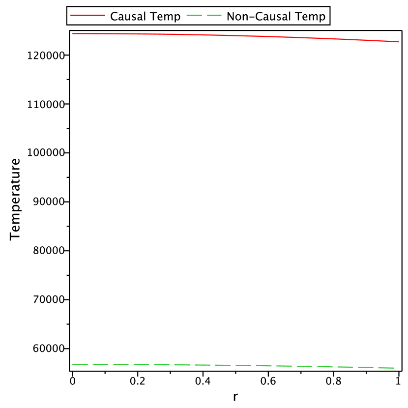
(c)

Figure 12: (a), (b) & (c) shows the plots of the temperature profiles of the collapsing stellar system w.r.t. radial coordinate $r$ for $\sigma=0$ and for $f(R)=R+\lambda R^{2}$ with $\lambda=5$, $f(R)=R^{1+\epsilon}$ with $\epsilon=0.01$ and $f(R)=R+\lambda\left[\exp\left(-\gamma R\right)-1\right]$ with $\lambda=0.1$ & $\gamma=0.0002$ respectively.

Using conditions in equation (55), the the causal heat transport equation (54) becomes

$$\beta T^{-\sigma}\left(qbs\right)_{,t}+q\,a\,b\,s = -\frac{\alpha\,\left(aT\right)_{,r}}{bs}\,\,T^{3-\sigma}.$$ (56)

The noncausal solution of the heat transport equation (56), with $\beta=0$ i.e. $\tau=0$ are [64]

$$\left(a\,T\right)^{4} = -\frac{4}{\alpha}\int a^{4}\,q\,b^{2}\,s^{2}\,dr+G(t),\hskip 45.52458pt\sigma=0$$ (57)

$$\ln\left(a\,T\right) = -\frac{1}{\alpha}\int q\,b^{2}\,s^{2}\,dr+G(t).\hskip 56.9055pt\sigma=4$$ (58)

The causal solution of the above heat transport equation (56) are [64]

$$\left(a\,T\right)^{4} = -\frac{4}{\alpha}\left[\beta\int a^{3}\,b\,s(q\,b\,s)_{,t}\,dr+\int a^{4}\,q\,b^{2}\,s^{2}\,dr\right]+G(t),\hskip 17.07182pt\sigma=0$$ (59)

$$\left(a\,T\right)^{4} = -\frac{4\beta}{\alpha}\exp\left(-\int\frac{4\,q\,b^{2}\,s^{2}}{\alpha}\,dr\right)\int a^{3}\,b\,s(q\,b\,s)_{,t}\,dr\,\exp\left(\int\frac{4\,q\,b^{2}\,s^{2}}{\alpha}\,dr\right)$$ (60)

$$+G(t)\exp\left(-\int\frac{4\,q\,b^{2}\,s^{2}}{\alpha}\,dr\right),\hskip 119.50148pt\sigma=4$$

where $G(t)$ appears as a function of integration and is determined by following boundary condition

$$\left(T^{4}\right)_{\Sigma} = \left(\frac{L_{\infty}}{4\pi\delta r^{2}b^{2}s^{2}}\right)_{\Sigma}.$$ (61)

where $L_{\infty}$ is the total luminosity for an observer at infinity given by (49) and $\delta>0$ is constant. The Figs. 12(a), 12(b) & 12(c) shows that for all these three $f(R)$ models under consideration, the stellar system deviates from thermodynamical equilibrium due to the relaxation effects. Also, the causal and noncausal temperature profiles differ inside the interior of the star and causal temperature remains greater than that of the non-causal temperature.

3 Discussion of the results

In this paper, we investigated the dynamics of a collapsing matter configuration in $f(R)$ gravity. The matter is assumed to be so massive that no stable compact objects like a white dwarf or a neutron star forms. The interior spacetime is smoothly matched to the outgoing radiation Vaidya metric across a timelike hypersurface. Incidentally, as has been noted earlier too, the matching conditions for the $f(R)$ gravity is highly restrictive, since the geometric variables which are to matched here not only includes induced metric and the extrinsic curvatures, but also the trace of the extrinsic curvatures, and the Ricci scalar along with it’s time derivative. However, we have shown that all these matching conditions can be carried out consistently, leading to a spacetime solution which admits a collapsing scenario in which the matter cloud radiates heat flux, in such a manner that the entire matter is radiated out without forming a black hole. Although similar solutions have been reported earlier for GR, our solution incorporates these features into the collapsing models of three particular $f(R)$ gravity models, while maintaining all the energy conditions. In particular, for all the three $f(R)$ theories we have analyzed physical quantities like energy density, in eqn. (62), radial pressure (63) and tangential pressure in eqn.(64), pressure anisotropy, in eqn. (36) and it can be seen from the Figs. 1(a), 1(b) & 1(c) , 2(a), 2(b) & 2(c) , 3(a), 3(b) & 3(c) , 4(a), 4(b) & 4(c) that they are regular and positive throughout the collapse. From Figs. 5(a), 5(b) & 5(c) it is also clear that the radial heat flux (65) is finite and positive throughout collapse. In particular, for $f(R)=R+\lambda R^{2}$, Figs. 7(a) and 11(a) show that both total luminosity and the effective adiabatic index are positive and increasing and have maximum value where luminosity is maximum. This behavior of the luminosity and adiabatic index can be interpreted as follows: an observer at rest at infinity will see a exponential radiating radial source until it reaches time when luminosity reaches its maximum value and then instantaneous turn off of the radial source. This happens since the total mass of the star radiates linearly as seen from the Fig. 6(b), and when the star reaches its maximum luminosity, there is no mass left to radiate and hence the observer at rest at infinity will see sudden turn off of the light source. The similar kind of behavior were obtained in GR too [75]. The Fig. 11(a) also shows that the effective adiabatic index is positive and less than $4/3$ which implies that the considered stellar system is unstable and represents a collapsing phenomena. Also note that the Figs. 8(a), 8(b) & 8(c) show that the energy conditions are positive and regular throughout the interior of the star.

For $f(R)=R^{1+\epsilon}$ and $f(R)=R+\lambda\,\left[\exp{(-\sigma R)}-1\right]$ similar behavior is obtained as well. For example, Figs. 11(b), and 11(c) shows that the effective adiabatic index is constant function of time, and is positive and less than $4/3$, and hence represents a collapsing scenario. We have shown graphically that the star radiates all its mass before reaching the singularity. So, there are no trapped surfaces formed during the collapse. This implies that neither a black hole nor a naked singularity exist at the end state of collapse. The Figs. 9(a), 9(b) & 9(c) and 10(a), 10(b) & 10(c) show that these model under consideration are physically viable. Also, the results obtained here reduces to those for GR for $f(R)=R$ [55].

Let us now comment on the nature of the central singularity. First, we note that the Ricci scalar (9) together with (44) imply that it diverges at $t=0$, when all the matter has been radiated away. So, naturally the question arises regarding the gravitational strength of the central curvature singularity (a strong singularity would imply a naked singularity). However, in the present case, the curvature scalars go as $t^{-2}$ which is precisely the sufficient condition for the singularity to be weak. So, our solutions represent a physically viable model where the spherically symmetric collapsing matter cloud undergoes gravitational collapse, which, during the collapse, also radiates away mass in the form of heat flux. The flux is radiated at such a rate that no horizon is ever formed and the central singularity is naked but gravitationally weak in nature.

Acknowledgments
The author AC is supported by the DST-MATRICS scheme of government of India through MTR/2019/000916 and by the DAE-BRNS Project No. 58/14/25/2019-BRNS.

Data availability
This manuscript has no associated data. This is a theoretical study and does not contain any experimental data.

Appendix

In this appendix, we give the detail expressions of the physical quantities of the collapsing matter cloud in terms of the metric functions. More precisely, we give the values for (10)-(13), and other quantities like the expansion scalar (8) and the Misner- Sharp mass function (27).

$$\rho = \frac{6FC_{3}C_{4}^{3}}{S_{1}C_{Z}^{2}t^{2}}\left[C_{1}-2C_{2}C_{3}\left(2C_{4}+C_{3}r^{2}\right)\right]^{2}+\frac{3\dot{s}\dot{F}}{s\,a^{2}}-\frac{F^{\prime\prime}}{b^{2}\,s^{2}}+\frac{f-R\,F}{2}-\frac{F^{\prime}}{b^{2}\,s^{2}}\left[\frac{b^{\prime}}{b}+\frac{2}{r}\right],$$ (62)

$$p_{r} = \frac{FC_{3}C_{4}^{2}}{S_{1}C_{Z}^{2}t^{2}}\left[2C_{1}C_{2}C_{3}\left(12C_{4}^{2}+4C_{3}C_{4}r^{2}-C_{3}r^{2}\right)-C_{1}^{2}\left(4C_{4}-C_{3}r^{2}\right)-8C_{2}^{2}C_{3}^{2}C_{4}\left(2C_{4}+C_{3}r^{2}\right)^{2}\right]$$ (63)

$$\leavevmode\nobreak\ \leavevmode\nobreak\ \leavevmode\nobreak\ \leavevmode\nobreak\ \leavevmode\nobreak\ \leavevmode\nobreak\ \leavevmode\nobreak\ \leavevmode\nobreak\ \leavevmode\nobreak\ \leavevmode\nobreak\ \leavevmode\nobreak\ \leavevmode\nobreak\ \leavevmode\nobreak\ \leavevmode\nobreak\ \leavevmode\nobreak\ \leavevmode\nobreak\ \leavevmode\nobreak\ \leavevmode\nobreak\ \leavevmode\nobreak\ \leavevmode\nobreak\ \leavevmode\nobreak\ \leavevmode\nobreak\ \leavevmode\nobreak\ \leavevmode\nobreak\ \leavevmode\nobreak\ \leavevmode\nobreak\ \leavevmode\nobreak\ \leavevmode\nobreak\ \leavevmode\nobreak\ \leavevmode\nobreak\ \leavevmode\nobreak\ \leavevmode\nobreak\ \leavevmode\nobreak\ \leavevmode\nobreak\ \leavevmode\nobreak\ \leavevmode\nobreak\ -\left(\frac{f-R\,F}{2}\right)-\frac{\dot{F}}{a^{2}}\left(\frac{\ddot{F}}{\dot{F}}+\frac{2\dot{s}}{s}\right)+\frac{F^{\prime}}{b^{2}\,s^{2}}\left(\frac{a^{\prime}}{a}+\frac{2}{r}+\frac{2b^{\prime}}{b}\right),$$

$$p_{t} = \frac{FC_{3}C_{4}^{2}}{S_{1}C_{Z}^{2}t^{2}}\left[C_{1}^{4}C_{4}^{2}\left(C_{3}r^{2}-4C_{4}\right)+2C_{1}^{3}C_{2}C_{3}C_{4}^{2}\left(-3C_{3}^{2}r^{4}+8C_{3}C_{4}r^{2}+28C_{4}^{2}\right)\right]+\frac{F^{\prime}}{r\,b^{2}\,s^{2}}$$ (64)

$$+ \frac{2FC_{1}^{2}C_{3}C_{4}^{2}}{S_{1}C_{Z}^{2}t^{2}}\left[\left(C_{3}r^{2}+2C_{4}\right)^{2}\left[6C_{2}^{2}C_{3}^{2}C_{4}^{2}\left(C_{3}r^{2}-6C_{4}\right)+C_{Z}^{2}\left(2C_{4}-C_{3}r^{2}\right)\right]\right]+\frac{F^{\prime}a^{\prime}}{a\,b^{2}\,s^{2}}$$

$$+ \frac{2FC_{1}C_{2}C_{3}^{2}C_{4}^{2}}{S_{1}C_{Z}^{2}t^{2}}\left[\left(C_{3}r^{2}+2C_{4}\right)^{3}\left[C_{Z}^{2}\left(C_{3}r^{2}-6C_{4}\right)-4C_{2}^{2}C_{3}^{2}C_{4}^{2}\left(C_{3}r^{2}-10C_{4}\right)\right]\right]+\frac{F^{\prime\prime}}{b^{2}\,s^{2}}$$

$$- \frac{8FC_{2}^{2}C_{3}^{3}C_{4}^{3}}{S_{1}C_{Z}^{2}t^{2}}\left[\left(C_{3}r^{2}+2C_{4}\right)^{4}\left(4C_{2}^{2}C_{3}^{2}C_{4}^{2}-C_{Z}^{2}\right)\right]-\left(\frac{f-R\,F}{2}\right)-\frac{\dot{F}}{a^{2}}\left(\frac{\ddot{F}}{\dot{F}}+\frac{2\dot{s}}{s}\right),$$

$$q = -\left[\frac{C_{4}^{5/2}C_{3}^{3/2}}{C_{Z}^{2}t^{3}}\frac{4\sqrt{2}rFC_{1}\left[4C_{2}C_{3}-\frac{2C_{1}}{C_{3}r^{2}+2C_{4}}\right]}{\left[C_{4}^{2}\left(4C_{2}C_{3}-\frac{2C_{1}}{C_{3}r^{2}+2C_{4}}\right)^{2}-4C_{Z}^{2}\right]^{3/2}}\right]+\frac{1}{a^{2}\,b^{2}\,s^{2}}\left[\dot{F}\,^{\prime}-\frac{\dot{F}a^{\prime}}{a}-\frac{\dot{s}\,F^{\prime}}{s}\right],$$ (65)

$$\Theta = \frac{6\sqrt{C_{3}C_{4}}}{t\sqrt{C_{4}^{2}\left(2C_{2}C_{3}-\frac{C_{1}}{C_{3}r^{2}+2C_{4}}\right)-2C_{Z}^{2}}},$$ (66)

$$m = \frac{8tr^{3}C_{3}C_{4}^{3}C_{Z}}{\left(C_{3}r^{2}+2C_{4}\right)^{3}}\,\left[\frac{2C_{2}C_{3}\left(C_{3}r^{2}+2C_{4}\right)-C_{1}}{2\left(C_{3}r^{2}+2C_{4}\right)\left(C_{2}C_{3}C_{4}^{2}-C_{Z}^{2}\right)-C_{1}C_{4}^{2}}\right],$$ (67)

$$S_{1} = C_{4}^{2}\left(2\,C_{2}\,C_{3}-{C_{1}}/\left({2\,C_{4}+C_{3}\,r^{2}}\right)\right)^{2}-C_{Z}^{2}.$$

References

- [1] S. W. Hawking and G. R. Ellis, The Large Scale Structure of Spacetime. Cambridge University Press, Cambridge 1975.
- [2] Robert M. Wald, General Relativity. University of Chicago Press, 1984.
- [3] P. S. Joshi, Gravitational Collapse and Spacetime Singularities. Cambridge University Press, Cambridge, England, 2007.
- [4] R. M. Wald, Quantum Field Theory in Curved Space-Time and Black Hole Thermodynamics, Chicago Lectures in Physics. University of Chicago Press, Chicago, IL, 10, 1995.
- [5] I. Buchbinder, S. Odintsov and I. Shapiro, Effective action in quantum gravity. IOP, Bristol, UK, 1992.
- [6] M. Reuter and F. Saueressig, Quantum Gravity and the Functional Renormalization Group: The Road towards Asymptotic Safety. Cambridge University Press, 2019.
- [7] M. B. Green, J. H. Schwarz and E. Witten, Superstring Theory. Vol. 1: Introduction, Cambridge Monographs in Mathematical Physics, 1987.
- [8] S. Capozziello, V. F. Cardone, S. Carloni and A. Troisi, Int. J. Mod. Phys. D 12, 1969 (2003).
- [9] S. Nojiri and S. D. Odintsov, Phys. Rev. D 68 (2003) 123512.
- [10] S.M. Carroll, V. Duvvuri, M. Trodden, M.S. Turner, Phys. Rev. B 70, 043528 (2004) .
- [11] H.A. Buchdahl, Month. Not. Royal Astron. Soc. 150 (1970) 1; J.D. Barrow, A.C. Ottewill, J. Phys. A: Math. Gen. 16 (1983) 2757.
- [12] T. Kobayashi and K. i. Maeda, Phys. Rev. D 78, 064019 (2008).
- [13] T. P. Sotiriou and V. Faraoni, Rev. Mod. Phys. 82, 451-497 (2010).
- [14] T. Clifton, P.G. Ferreira, A. Padilla, C. Skordis, Phys. Rep. 513, 1 (2012).
- [15] T.P. Sotiriou, V. Faraoni, Rev. Mod. Phys. 82, 451 (2010).
- [16] S. Capozziello, M. De Laurentis, S. D. Odintsov and A. Stabile, Phys. Rev. D 83 (2011) 064004.
- [17] S. Capozziello, M. De Laurentis, I. De Martino, M. Formisano and S. D. Odintsov, Phys. Rev. D 85 (2012) 044022.
- [18] A. V. Astashenok, S. Capozziello and S. D. Odintsov, JCAP 12, 040 (2013).
- [19] S. Nojiri, S.D. Odintsov, Phys. Rep. 505, 59 (2011).
- [20] S. Nojiri, S.D. Odintsov, V.K. Oikonomou, Phys. Rep. 692, 1 (2017).
- [21] C. J. S. Clarke, “The Analysis of space-time singularities,” CUP, 1993.
- [22] A. De Felice and S. Tsujikawa, Living Rev. Rel. 13, 3 (2010).
- [23] E. Babichev and D. Langlois, Phys. Rev. D 80, 121501 (2009) [erratum: Phys. Rev. D 81, 069901 (2010)].
- [24] A. Cooney, S. DeDeo and D. Psaltis, Phys. Rev. D 82, 064033 (2010).
- [25] A. V. Astashenok, S. D. Odintsov and A. de la Cruz-Dombriz, Class. Quant. Grav. 34, no.20, 205008 (2017).
- [26] R. Abbott et al. [LIGO Scientific and Virgo], Astrophys. J. Lett. 896, no.2, L44 (2020).
- [27] A. V. Astashenok, S. Capozziello, S. D. Odintsov and V. K. Oikonomou, Phys. Lett. B 811, 135910 (2020).
- [28] A. V. Astashenok, S. Capozziello, S. D. Odintsov and V. K. Oikonomou, [arXiv:2103.04144 [gr-qc]].
- [29] A. Chatterjee, A. Ghosh and S. Jaryal, Phys. Rev. D 102, no.6, 064048 (2020).
- [30] K. Bamba, S. Nojiri and S. D. Odintsov, Phys. Lett. B 698, 451 (2011).
- [31] E. V. Arbuzova and A. D. Dolgov, Phys. Lett. B 700, 289 (2011).
- [32] M. Sharif, H.R. Kausar, Astrophys. Space Sci. 331, 281 (2011).
- [33] R. Goswami, A.M. Nzioki, S.D. Maharaj, S.G. Ghosh, Phys. Rev. D 90, 084011 (2014).
- [34] S. Chakrabarti and N. Banerjee, Gen. Relativ. Gravit. 48, 57 (2016).
- [35] S. Chakrabarti and N. Banerjee, Eur. Phys. J. Plus. 131, 144 (2016).
- [36] A. V. Astashenok, K. Mosani, S. D. Odintsov and G. C. Samanta, Int. J. Geom. Meth. Mod. Phys. 16, no.03, 1950035 (2019).
- [37] G. Abbas, M. S. Khan, Z. Ahmad and M. Zubair, Eur. Phys. J. C 77, no.7, 443 (2017).
- [38] S. Chakrabarti, R. Goswami, S. D. Maharaj and N. Banerjee, Gen. Relativ. Gravit. 50, 148 (2018).
- [39] G. Abbas and H. Nazar, Int. J. Mod. Phys. A 34(33), 1950220 (2019).
- [40] M. Sharif, Z. Yousaf, Eur. Phys. J. C 73, 2633 (2013).
- [41] M. Sharif, Z. Yousaf, Phys. Rev. D 88, 024020 (2013).
- [42] H.R. Kausar and I. Noureen, Eur. Phys. J. C 74, 2760 (2014).
- [43] A. Borisov, B. Jain, P. Zhang, Phys. Rev. D 85, 063518 (2012).
- [44] J. Guo, D. Wang, A.V. Frolov, Phys. Rev. D 90, 024017 (2014).
- [45] A.A. Starobinsky, Phys. Lett. B. 91, 99 (1980).
- [46] G. Cognola, E. Elizalde, S. Nojiri, S. D. Odintsov, L. Sebastiani and S. Zerbini, Phys. Rev. D 77, 046009 (2008).
- [47] P.C. Vaidya, Proc. Indian Acad. Sci. A 33, 264 (1951).
- [48] N. O. Santos, MNRAS, 216, 403 (1985).
- [49] L. P. Eisenhart, Riemannian Geometry. Princeton University Press, Princeton, 1925.
- [50] J. Eiesland, Trans. Am. Math. Soc. 27, 213 (1925).
- [51] K.R. Karmarkar, Proc. Indian Acad. Sci. A 27, 56 (1948).
- [52] K.N. Singh, N. Pant, Eur. Phys. J. C 76, 524 (2016).
- [53] N.F. Naidu, M. Govender, S.D. Maharaj, Eur. Phys. J. C 78, 48 (2018).
- [54] M. Govender, A. Maharaj, K. N. Singh and N. Pant, Mod. Phys. Lett. A 35, no.20, 2050164 (2020).
- [55] S.C. Jaryal, Eur. Phys. J. C 80, 683 (2020).
- [56] R. Maartens, Class. Quantum Gravity 12, 1455 (1995).
- [57] J. Martinez, Phys. Rev. D 53, 6921 (1996).
- [58] A. Di Prisco, L. Herrera, M. Esculpi, Class. Quantum Grav. 13, 1053 (1996).
- [59] L. Herrera, A. Di Prisco, J.L. Hernandez-Pastora, J. Martin and J. Martinez, Class. Quantum Grav. 14, 2239 (1997).
- [60] L. Herrera and N. O. Santos, Mon. Not. R. Astron. Soc. 287, 161 (1997).
- [61] M. Govender, S.D. Maharaj, R. Maartens, Class. Quant. Grav. 15, 323 (1998).
- [62] M. Govender, R. Maartens, S.D. Maharaj, Mon. Not. Roy. Astron. Soc. 310, 557 (1999).
- [63] R. Maartens, M. Govender, S.D. Maharaj, Gen. Relativ. Grav. 31, 815 (1999).
- [64] M. Govender and K. Govinder, Phys. Lett. A283, 71 (2001).
- [65] N. Deruelle, M. Sasaki and Y. Sendouda, Prog. Theor. Phys. 119, 237-251 (2008).
- [66] J. M. M. Senovilla, Phys. Rev. D 88, 064015 (2013).
- [67] C. W. Misner and D. H. Sharp, Phys. Rev. 136, B571 (1964).
- [68] M. E. Cahill, G.C. McVittie, J. Math. Phys. 11, 1382 (1970).
- [69] A. Banerjee, S. Chatterjee, N. Dadhich, Mod. Phys. Lett. A 17, 2335 (2002).
- [70] K. Schwarzschild, Phys.-Math. Klasse, 189 (1916).
- [71] J. Ospino, L.A. Nez, Eur. Phys. J. C 80, 166 (2020).
- [72] R. Chan MNRAS, 288, 589 (1997). ; R, Chan, MNRAS, 299, 811 (1998).
- [73] S. Chandrasekhar, Astrophys. J. 140, 417 (1964).
- [74] L. Herrera, Phys. Lett. A 165, 206 (1992).
- [75] G. Pinheiro, R. Chan, Gen. Relat. Gravit.43, 1451 (2011).
- [76] L. Herrera and N. O. Santos, Phys. Rev. D 70, 084004 (2004); L. Herrera, G. Le Denmat, N. O. Santos, A. Wang, Int. J. Mod. Phys. D 13, 583 (2004); L. Herrera, Int. J. Mod. Phys. D 15, 2197 (2006).
- [77] W. Israel and J. Stewart, Ann. Phys.(N.Y.), 118, 341 (1979).