Energy-conserving integrator for conservative Hamiltonian systems with ten-dimensional phase space

Abstract

In this paper, an implicit nonsymplectic exact energy-preserving integrator is specifically designed for a ten-dimensional phase-space conservative Hamiltonian system with five degrees of freedom. It is based on a suitable discretization-averaging of the Hamiltonian gradient, with a second-order accuracy to numerical solutions. A one-dimensional disordered discrete nonlinear Schrödinger equation and a post-Newtonian Hamiltonian system of spinning compact binaries are taken as our two examples. We demonstrate numerically that the proposed algorithm exhibits good long-term performance in the preservation of energy, if roundoff errors are neglected. This result is independent of time steps, initial orbital eccentricities, and regular and chaotic orbital dynamical behavior. In particular, the application of appropriately large time steps to the new algorithm is helpful in reducing time-consuming and roundoff errors. This new method, combined with fast Lyapunov indicators, is well suited related to chaos in the two example problems. It is found that chaos in the former system is mainly responsible for one of the parameters. In the latter problem, a combination of small initial separations and high initial eccentricities can easily induce chaos.

Unified Astronomy Thesaurus concepts: Black hole physics (159); Computational methods (1965); Computational astronomy (293); Celestial mechanics (211)

1 Introduction

Recently, several gravitational-wave signals (e.g. GW150914 and GW190521) emitted from binary black hole mergers were successfully detected (Abbott et al. 2016, 2020a, 2020b). These are consistent with the predictions of Einstein’s theory of general relativity. The black holes’ masses and spins were also inferred from the observed data. The post-Newtonian (PN) expansion of the relativistic two-body dynamics (Blanchet et al. 1995; Buonanno $\&$ Damour 1999; Blanchet 2014) is suitable for describing theoretical templates of the early inspiral gravitational waveforms. The known PN equations of motion are accurate to $O((v/c)^{6})$ [i.e., third post-Newtonian (3PN) order], and are even accurate to $O((v/c)^{7})$ (Blanchet 2014), where the orbital velocity, $v$, is small, as compared with the speed of light, $c$. Harmonic-coordinate Lagrangian formalism and ADM-coordinate Hamiltonian formalism were independently applied to provide the PN equations of motion. On the basis of the Legendre transform, the former formalism can be transformed into the latter; inversely, the former formalism can also be derived from the latter. This being the case, Damour et al. (2001a) and de Andrade et al. (2001) claimed that the two methods for describing the motion of two compact bodies are physically equivalent. Higher-order PN terms are truncated in general when one of the two PN formalisms is derived from another. This fact shows that the two PN formalisms have some differences (Wu et al. 2015; Wu $\&$ Huang 2015). The coherent non-truncated equations of motion derived from a PN Lagrangian also differ slightly differ from the truncated equations of motion derived from the PN Lagrangian (Li et al. 2019, 2020). Specifically, some small differences always exist between the coherent Lagrangian equations, the truncated Lagrangian equations, and the Hamiltonian at the same PN order. In some circumstances, such small differences cause the three PN presentations to have complete different orbital dynamical behavior in terms of order and chaos.

When the black hole binaries are non-spinning, the PN equations of motion are analytically integrable and solvable from a theoretical point of view. However, the analytical solutions of the PN equations are difficult to be written as explicit functions of time. If the bodies are spinning, the PN equations of motion become non-integrable. The binaries may even exhibit chaos for the description of a dynamical system exhibiting sensitive dependence to initial conditions. The onset of chaos may affect a matched filtering method requiring theoretical templates of gravitational waves that agree with experimental gravitational-wave signals, without noise. On the other hand, it can enhance the signals, in which case it may be helpful to observe the gravitational waves (Levin 1999; Cornish $\&$ Levin 2002). Considering the fact that chaos may make either a positive or negative contribution to the detection of the waveforms, several authors have focused on the chaotic dynamics of spinning black hole binaries (Schnittman $\&$ Rasio 2001; Königsdörffer $\&$ Gopakumar 2005; Gopakumar $\&$ Königsdörffer 2005; Levin 2006; Wu $\&$ Huang 2015) finding chaos in some cases (Levin 2000; Levin 2003; Cornish $\&$ Levin 2003; Hartl $\&$ Buonanno 2005; Wu $\&$ Xie 2007, 2008; Wang $\&$ Wu 2011; Huang et al. 2014; Wu et al. 2015; Huang et al. 2016). In the presence of chaos, analytically solving the PN equations of motion for the systems of spinning black hole binaries analytically is impossible.

Analytically solving the PN equations of motion presents considerable difficulties, regardless of whether the binaries are spinning or not. However, numerically solving the PN equations is very easy and convenient. Conventional integrators, such as Runge-Kutta methods, often lead to an increase in energy errors with time, and very poor energy accuracy in long integration time, so that the obtained results are unreliable. At this point, a note is worthwhile on the subject of energy conservation. In fact, energy conservation is essential in numerical integration. It is a fundamental property inherent in conservative Hamiltonian flow. In addition, it is often used to check numerical accuracy, although it is not always completely reliable in obtaining high-precision results. Enforcing the conservation of energy significantly improves the quality of orbit integrations in many situations. Below, we introduce three paths for energy conservation.

Smplectic integrators (Wisdom 1982; Ruth 1983) preserve the original Hamiltonian flow. They do not exactly conserve the real Hamiltonian or energy, but they cause the energy to oscillate. Specifically, they show no secular energy drift, causing the energy errors to remain bounded. As such, symplectic integrators are regarded to be energy-conserving. Due to these good properties, symplectic integrators, such as the second-order symplectic method of Wisdom $\&$ Holman (1991), are widely used in the long-term integration of celestial N-body problems in the solar system. Explicit symplectic methods are less expensive than implicit methods, and therefore have priority in terms of application. However, they are not available to relativistic or PN problems in general, as either the variables in the systems are inseparable, or two integrable splitting parts can be given to the systems, but their analytical solutions are not explicit functions of time. As a result, implicit symplectic algorithms, such as the implicit midpoint rule (Feng 1986), are considered. Explicit and implicit symplectic composition methods (Liao 1997; Preto $\&$ Saha 2009; Lubich et al. 2010; Mei et al. 2013a) are superior to completely implicit symplectic integrators with respect to computational efficiency. Such a construction was encountered in the simulation of the PN Hamiltonian dynamics of spinning compact binaries (Zhong et al. 2010; Mei et al. 2013b). More recently, explicit symplectic integrators were proposed for Schwarzschild spacetime geometry, whose Hamiltonian can be split into four integrable parts, with analytical solutions as explicit functions of proper time (Wang et al. 2021a). They are also applicable to the Hamiltonian of Reissner-Nordström black holes (Wang et al. 2021b). On the other hand, the extended phase-space explicit methods employed by Pihajoki (2015) in relation to inseparable Hamiltonian problems possess energy conservation, similarly to symplectic methods. Permutations of coordinates and/or momenta have been optimized by Liu et al. (2016) and Luo et al. (2017).

The manifold correction scheme of Nacozy (1971) pulls the numerical solution (given by a conventional integrator) back to the original manifold of constant energy along the least-squares shortest path. The corrected solution approximately satisfies the constant energy; it can cause the energy to be accurate to a machine double-precision if the integrator provides a machine single-precision to the energy. Using integral invariant relations, this approach has been extended to adjust the integrated position and velocity so as to approximately satisfy the varying Kepler energy, Laplace integral, and/or angular momentum vector for each of the N bodies in the solar system (Wu et al. 2007; Ma et al. 2008a). The least-squares correction approach has also proven applicable to the numerical correction of all integrals in the conservative PN Hamiltonian formulation of spinning compact binaries (Zhong $\&$ Wu 2010). In terms of scale transformations, Nacozy’s idea was also further developed to rigorously satisfy the varying Kepler energy, Laplace integral, and/or angular momentum vector at every integration step (Fukushima 2003a, 2003b, 2003c, 2004; Ma et al. 2008b). The velocity-scaling correction method has been applied to nonconservative or dissipative restricted three-body problems (Wang et al. 2016, 2018). Recently, the Kepler solver was used to rigorously conserve all integrals and orbital elements (with the exception of the mean longitude) of quasi-Keplerian orbits (Deng et al. 2020). These correction schemes have been shown to significantly suppress the growth of integration errors, and to dramatically enhance the quality of the integrations.

In addition to a variety of correction schemes, a class of energy-preserving numerical integration methods can exactly preserve the energies of Hamiltonian systems. These are obtained by suitably discretizing the canonical equations of Hamiltonian systems. Chorin et al. (1978) constructed an energy-conserving algorithm for the discretization of Hamiltonian gradients with a first-order accuracy to the numerical solutions. A similar integrator was also proposed by Feng (1985). A second-order approximation to the Hamiltonian gradient has been designed for a four-dimensional phase-space Hamiltonian system (Qin 1987; Itoh $\&$ Abe 1988). Here, each component of the Hamiltonian gradient is an average of four difference terms, each of which is the ratio of the increment of the Hamiltonian between positions (or momenta) to the position (or momentum) increment. Such discretization-averaging of the Hamiltonian equations is complex, because it depends on the dimension of a Hamiltonian phase space. Bacchini et al. (2018, 2019) established a precise energy-conserving implicit integration scheme for six-dimensional phase-space Hamiltonian problems, and simulated time-like (massive particles) and null (photons) geodesics in Schwarzschild and Kerr spacetimes. This idea was then generalized to the eight-dimensional phase-space PN Hamiltonian dynamics of compact binaries with one body spinning (Hu et al. 2019). These energy-conserving schemes are based on the coordinate-increment discrete gradient (Robert et al. 1999). They can also be constructed in terms of the mean value discrete gradient (Harten 1983; Quispel $\&$ McLaren 2008; Huang $\&$ Mei 2020) and the midpoint discrete gradient (Gonzalez 1996).

Following on from our previous work (Hu et al. 2019), we introduce a new energy-conserving algorithm for a ten-dimensional phase-space PN Hamiltonian of black hole binaries. This scheme gives second-order approximations to numerical solutions. This is the main aim of this paper. The remainder of this paper is organized as follows: in Section 2, we describe how to construct an energy-conserving method for ten-dimensional phase-space Hamiltonian problems. Taking a one-dimensional disordered discrete nonlinear Schrödinger equation (Skokos et al. 2014; Senyange et al. 2018) as an example, we evaluate the numerical performance of the new algorithm. The new method is applied to study the dynamical properties of the system in Section 3. For comparison, the Runge-Kutta method, the implicit midpoint method (Feng 1986; Zhong et al. 2010; Mei et al. 2013a), and an extended phase-space symplectic-like algorithm (Pihajoki 2015; Liu et al. 2016; Li $\&$ Wu 2017; Luo et al. 2017) are also used. In Section 4, we choose a PN Hamiltonian of spinning compact binaries as another example with which to verify the algorithmic performance. The new method is used to investigate the regular and chaotic dynamical behavior of orbits in the PN problem. Section 5 summarises our main results and conclusions. The new method is shown to obtain the numerical solutions, accurate to the second order, in the Appendix.

2 Construction of new energy-conserving method

Let $\bm{q}$ and $\bm{p}$, respectively, be $N$-dimensional generalized coordinate and conjugate momentum vectors in a $2N$-dimensional conservative Hamiltonian system, $H(\bm{q},\bm{p})$. This Hamiltonian corresponds to the following canonical equations:

$$\dot{\bm{q}}=\frac{\partial{\emph{H}}}{\partial{\bm{p}}},$$ (1)

$$\dot{\bm{p}}=-\frac{\partial{\emph{H}}}{\partial{\bm{q}}}.$$ (2)

Taking time step $h=t_{n+1}-t_{n}$ and discretizing the canonical equations, we obtain the relationship between the solution $(p_{n},q_{n})$ at the $n$th step, and the solution $(p_{n+1},q_{n+1})$ at the $(n+1)$th step as follows:

$$\frac{\bm{q}_{n+1}-\bm{q}_{n}}{h}=\frac{H(\bm{q}_{n},\bm{p}_{n+1})-H(\bm{q}_{n},\bm{p}_{n})}{\bm{p}_{n+1}-\bm{p}_{n}},$$ (3)

$$\frac{\bm{p}_{n+1}-\bm{p}_{n}}{h}=-\frac{H(\bm{q}_{n+1},\bm{p}_{n+1})-H(\bm{q}_{n},\bm{p}_{n+1})}{\bm{q}_{n+1}-\bm{q}_{n}}.$$ (4)

It can be derived from Equations (3) and (4) that

$$H(\bm{q}_{n+1},\bm{p}_{n+1})=H(\bm{q}_{n},\bm{p}_{n}).$$ (5)

This result shows that Equations (3) and (4) are an exact energy-conserving algorithm, which provides the solution $(p_{n+1},q_{n+1})$ at the $(n+1)$th step, after the solution $(p_{n},q_{n})$ at the $n$th step advances the time step, $h$. In general, the solution is implicitly given. In this case, the use of a certain iteration method is necessary.

In fact, the above energy-conserving method belongs to a Hamiltonian-conserving method, which is only viewed as a first-order approximation to the Hamiltonian gradient. It therefore provides a first-order accuracy to the numerical solutions. In fact, there is also a second-order Hamiltonian-conserving scheme for four-dimensional phase-space Hamiltonian systems (Qin 1987; Itoh $\&$ Abe 1988; Feng $\&$ Qin 2009), as discussed in the introduction. In that algorithmic construction, a second-order discrete approximation to the Hamiltonian gradient is an average of four Hamiltonian difference terms. The average becomes more complicated as the dimensionality of the Hamiltonian increases.

Following on from previous work of Hu et al. (2019), we consider the construction of a Hamiltonian-conserving scheme for a ten-dimensional phase-space conservative system. For simplicity, 0 and 1 respectively correspond to the numbers of integration steps, $n$ and $(n+1)$; e.g. $H(q_{1(n+1)}$, $q_{2(n+1)}$, $q_{3(n+1)}$, $q_{4(n+1)}$, $q_{5(n+1)}$, $p_{1(n+1)}$, $p_{2(n+1)}$, $p_{3(n+1)}$, $p_{4(n+1)}$, $p_{5(n+1)})/$ $(p_{1(n+1)}-p_{1(n)})$ = $H(1111111111)/(p_{11}-p_{10})$. Equations (1) and (2) are discretized in the following forms:

$$\frac{q_{11}-q_{10}}{h}=\frac{1}{10}\frac{1}{p_{11}-p_{10}}$$ (6)

$$\times\left[H(0000010000)-H(0000000000)\right.$$

$$+H(1000010000)-H(1000000000)$$

$$+H(0000110001)-H(0000100001)$$

$$+H(1100011000)-H(1100001000)$$

$$+H(0001110011)-H(0001100011)$$

$$+H(1110011100)-H(1110001100)$$

$$+H(0011110111)-H(0011100111)$$

$$+H(1111011110)-H(1111001110)$$

$$+H(0111111111)-H(0111101111)$$

$$\left.+H(1111111111)-H(1111101111)\right],$$

$$\frac{q_{21}-q_{20}}{h}=\frac{1}{10}\frac{1}{p_{21}-p_{20}}$$ (7)

$$\times\left[H(0000001000)-H(0000000000)\right.$$

$$+H(0100001000)-H(0100000000)$$

$$+H(1000011000)-H(1000010000)$$

$$+H(0110001100)-H(0110000100)$$

$$+H(1000111001)-H(1000110001)$$

$$+H(0111001110)-H(0111000110)$$

$$+H(1001111011)-H(1001110011)$$

$$+H(0111101111)-H(0111100111)$$

$$+H(1011111111)-H(1011110111)$$

$$\left.+H(1111111111)-H(1111110111)\right],$$

$$\frac{q_{31}-q_{30}}{h}=\frac{1}{10}\frac{1}{p_{31}-p_{30}}$$ (8)

$$\times\left[H(0000000100)-H(0000000000)\right.$$

$$+H(0010000100)-H(0010000000)$$

$$+H(0100001100)-H(0100001000)$$

$$+H(0011000110)-H(0011000010)$$

$$+H(1100011100)-H(1100011000)$$

$$+H(0011100111)-H(0011100011)$$

$$+H(1100111101)-H(1100111001)$$

$$+H(1011110111)-H(1011110011)$$

$$+H(1101111111)-H(1101111011)$$

$$\left.+H(1111111111)-H(1111111011)\right],$$

$$\frac{q_{41}-q_{40}}{h}=\frac{1}{10}\frac{1}{p_{41}-p_{40}}$$ (9)

$$\times\left[H(0000000010)-H(0000000000)\right.$$

$$+H(0001000010)-H(0001000000)$$

$$+H(0010000110)-H(0010000100)$$

$$+H(0001100011)-H(0001100001)$$

$$+H(0110001110)-H(0110001100)$$

$$+H(1001110011)-H(1001110001)$$

$$+H(1110011110)-H(1110011100)$$

$$+H(1101111011)-H(1101111001)$$

$$+H(1110111111)-H(1110111101)$$

$$\left.+H(1111111111)-H(1111111101)\right],$$

$$\frac{q_{51}-q_{50}}{h}=\frac{1}{10}\frac{1}{p_{51}-p_{50}}$$ (10)

$$\times\left[H(0000000001)-H(0000000000)\right.$$

$$+H(0000100001)-H(0000100000)$$

$$+H(0001000011)-H(0001000010)$$

$$+H(1000110001)-H(1000110000)$$

$$+H(0011000111)-H(0011000110)$$

$$+H(1100111001)-H(1100111000)$$

$$+H(0111001111)-H(0111001110)$$

$$+H(1110111101)-H(1110111100)$$

$$+H(1111011111)-H(1111011110)$$

$$\left.+H(1111111111)-H(1111111110)\right],$$

$$\frac{p_{11}-p_{10}}{h}=-\frac{1}{10}\frac{1}{q_{11}-q_{10}}$$ (11)

$$\times\left[H(1000000000)-H(0000000000)\right.$$

$$+H(1000010000)-H(0000010000)$$

$$+H(1100001000)-H(0100001000)$$

$$+H(1000110001)-H(0000110001)$$

$$+H(1110001100)-H(0110001100)$$

$$+H(1001110011)-H(0001110011)$$

$$+H(1111001110)-H(0111001110)$$

$$+H(1011110111)-H(0011110111)$$

$$+H(1111101111)-H(0111101111)$$

$$\left.+H(1111111111)-H(0111111111)\right],$$

$$\frac{p_{21}-p_{20}}{h}=-\frac{1}{10}\frac{1}{q_{21}-q_{20}}$$ (12)

$$\times\left[H(0100000000)-H(0000000000)\right.$$

$$+H(0100001000)-H(0000001000)$$

$$+H(0110000100)-H(0010000100)$$

$$+H(1100011000)-H(1000011000)$$

$$+H(0111000110)-H(0011000110)$$

$$+H(1100111001)-H(1000111001)$$

$$+H(0111100111)-H(0011100111)$$

$$+H(1101111011)-H(1001111011)$$

$$+H(1111110111)-H(1011110111)$$

$$\left.+H(1111111111)-H(1011111111)\right],$$

$$\frac{p_{31}-p_{30}}{h}=-\frac{1}{10}\frac{1}{q_{31}-q_{30}}$$ (13)

$$\times\left[H(0010000000)-H(0000000000)\right.$$

$$+H(0010000100)-H(0000000100)$$

$$+H(0011000010)-H(0001000010)$$

$$+H(0110001100)-H(0100001100)$$

$$+H(0011100011)-H(0001100011)$$

$$+H(1110011100)-H(1100011100)$$

$$+H(1011110011)-H(1001110011)$$

$$+H(1110111101)-H(1100111101)$$

$$+H(1111111011)-H(1101111011)$$

$$\left.+H(1111111111)-H(1101111111)\right],$$

$$\frac{p_{41}-p_{40}}{h}=-\frac{1}{10}\frac{1}{q_{41}-q_{40}}$$ (14)

$$\times\left[H(0001000000)-H(0000000000)\right.$$

$$+H(0001000010)-H(0000000010)$$

$$+H(0001100001)-H(0000100001)$$

$$+H(0011000110)-H(0010000110)$$

$$+H(1001110001)-H(1000110001)$$

$$+H(0111001110)-H(0110001110)$$

$$+H(1101111001)-H(1100111001)$$

$$+H(1111011110)-H(1110011110)$$

$$+H(1111111101)-H(1110111101)$$

$$\left.+H(1111111111)-H(1110111111)\right],$$

$$\frac{p_{51}-p_{50}}{h}=-\frac{1}{10}\frac{1}{q_{51}-q_{50}}$$ (15)

$$\times\left[H(0000100000)-H(0000000000)\right.$$

$$+H(0000100001)-H(0000000001)$$

$$+H(1000110000)-H(1000010000)$$

$$+H(0001100011)-H(0001000011)$$

$$+H(1100111000)-H(1100011000)$$

$$+H(0011100111)-H(0011000111)$$

$$+H(1110111100)-H(1110011100)$$

$$+H(0111101111)-H(0111001111)$$

$$+H(1111111110)-H(1111011110)$$

$$\left.+H(1111111111)-H(1111011111)\right].$$

On the right-hand sides of Equations (6)-(15), each component of the Hamiltonian gradient is approximately expressed in terms of an average of 10 Hamiltonian differences. Using (6)-(15), we simply derive the relation

$$H(1111111111)-H(0000000000)=0.$$ (16)

This fact indicates that Equations (6)-(15) strictly preserve the Hamiltonian energy from the theoretical viewpoint. This construction is a new energy-conserving algorithm, with a coordinate-increment discrete gradient. In fact, this method gives a second-order accuracy to the numerical solutions. Itoh $\&$ Abe (1988) provided a simple explanation as to why a similar energy-conserving method for a four-dimensional phase-space Hamiltonian problem is accurate to the order of $h^{2}$. We also provide a detailed explanation for Equations (6)-(15), with the numerical solutions accurate to this order, in the Appendix.

Below, the efficiency of the new energy-conserving algorithm is verified, base on simulations of two dynamical models.

3 One-dimensional disordered discrete nonlinear Schrödinger equation

A one-dimensional disordered discrete nonlinear Schrödinger equation (DDNLS) is considered in Section 3.1. The performance of the newly proposed energy-conserving algorithm is then checked in Section 3.2. We use our new method, combined with the technique of fast Lyapunov indicators (Froeschlé et al. 1997; Froeschlé $\&$ Lega 2000; Wu et al. 2006) to provide an insight into the influences of some dynamical parameters on orbital dynamics in Section 3.3.

3.1 Model

DDNLS describes the motion of coupled, nonlinear oscillators in a crystal lattice. The so-called “one-dimension” in the model refers to the geometric dimensionality of the model being 1, i.e., the dynamical evolution in the nonlinear partial differential Schrödinger equation with respect to one position variable. However, the canonical variables of the model can be expanded to any dimensions in a Hamiltonian from the discretized Schrödinger equation. DDNLS corresponds to the following dimensionless Hamiltonian (Skokos et al. 2014; Senyange et al. 2018)

$$H(\bm{q},\bm{p}) = \sum_{m=1}^{N}[\frac{\varepsilon_{m}}{2}\left(q_{m}^{2}+p_{m}^{2}\right)+\frac{\beta}{8}\left(q_{m}^{2}+p_{m}^{2}\right)^{2}$$ (17)

$$-\left(p_{m}p_{m+1}+q_{m}q_{m+1}\right)].$$

Here, $\varepsilon_{m}$ are random on-site energies in the interval $[-W/2,W/2]$, where $W$ represents a disorder strength of the system, and $\beta\geq 0$ is a nonlinearity strength. Taking $N=5$, and boundary conditions $q_{0}=p_{0}=q_{N+1}=p_{N+1}=0$, we rewrite the Hamiltonian as

$$H(q_{1},q_{2},q_{3},q_{4},q_{5},p_{1},p_{2},p_{3},p_{4},p_{5})$$ (18)

$$=\frac{\varepsilon_{1}}{2}{}(q_{1}^{2}+p_{1}^{2})+\frac{\beta}{8}{}(q_{1}^{2}+p_{1}^{2})^{2}-(p_{1}p_{2}+q_{1}q_{2})$$

$$+\frac{\varepsilon_{2}}{2}{}(q_{2}^{2}+p_{2}^{2})+\frac{\beta}{8}{}(q_{2}^{2}+p_{2}^{2})^{2}-(p_{2}p_{3}+q_{2}q_{3})$$

$$+\frac{\varepsilon_{3}}{2}{}(q_{3}^{2}+p_{3}^{2})+\frac{\beta}{8}{}(q_{3}^{2}+p_{3}^{2})^{2}-(p_{3}p_{4}+q_{3}q_{4})$$

$$+\frac{\varepsilon_{4}}{2}{}(q_{4}^{2}+p_{4}^{2})+\frac{\beta}{8}{}(q_{4}^{2}+p_{4}^{2})^{2}-(p_{4}p_{5}+q_{4}q_{5})$$

$$+\frac{\varepsilon_{5}}{2}{}(q_{5}^{2}+p_{5}^{2})+\frac{\beta}{8}{}(q_{5}^{2}+p_{5}^{2})^{2}.$$

In addition to the Hamiltonian as an integral of energy, the norm

$$Q=\sum_{m=1}^{5}\frac{1}{2}\left(q_{m}^{2}+p_{m}^{2}\right).$$ (19)

remains invariant (Skokos et al. 2014).

3.2 Numerical evaluations

When Equations (6)-(15) are applied to the system (18), we call this algorithm EC. For comparison, the same-order Runge-Kutta method (RK) in Equations (A6) and (A7), the implicit midpoint method (IS) in Equations (A10) and (A11), and the extended phase-space symplectic-like algorithm (ES) (Pihajoki 2015; Liu et al. 2016; Li $\&$ Wu 2017; Luo et al. 2017) are independently used to integrate the system. The time step is given by $h=0.01$. Orbits 1 and 2 have the same initial conditions, $q_{i}=(6-i)/10$ and $p_{i}=0$. Parameters $\varepsilon_{m}=0$ are the same. However, $\beta=1$ for Orbit 1, and $\beta=10$ for Orbit 2.

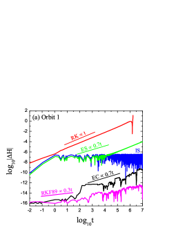
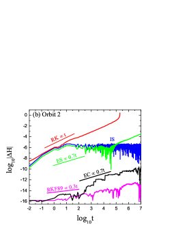
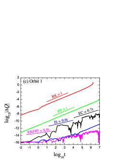
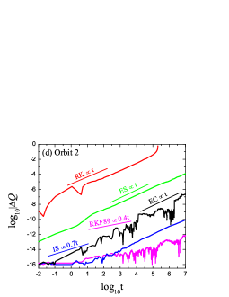
Figure 1: Errors of the Hamiltonian and norm, $\Delta H$ and $\Delta Q$, for the five algorithms solving Orbit 1 and Orbit 2 in the ten-dimensional phase-space DDNLS system. The time step is $h=0.01$. Orbits 1 and 2 have the same initial conditions, where $q_{i}=(6-i)/10$ and $p_{i}=0$. The two orbits take the same values, $\varepsilon_{m}=\varepsilon=0$. $\beta=1$ for Orbit 1, and $\beta=10$ for Orbit 2. The slope of the error growth with time is marked for each algorithm. When the integration time $t=10^{7}$ corresponds to $10^{9}$ integration steps, the implicit symplectic midpoint method IS causes the Hamiltonian errors to have no secular drift. Although the Hamiltonian errors of the new energy-conserving method EC, yield a slightly secular growth, they are smaller than those of IS, and are approximate to those of the high-precision method, RKF89.

Figures 1 (a) and (b) plot the Hamiltonian errors for the four algorithms solving Orbits 1 and 2. When the integration time reaches $t=10^{7}$ corresponding to $10^{9}$ steps, the Hamiltonian errors calculated by the RK method grow linearly with time for the two orbits. They are larger than those given by the IS or ES method. The errors remain bounded and stable for IS. However, ES gives a secular drift to the energy errors after $t=10^{4}$. This may be due to the use of a slightly larger step size. In fact, this drift is absent if $h=0.001$. Clearly, the EC method shows the smallest errors with slight secular growths, as compared with the other three algorithms. The errors for EC are approximate to those for an eighth- and ninth-order Runge–Kutta–Fehlberg integrator [RKF89] with adaptive step sizes. Without doubt, the Hamiltonian or energy is conserved by the IS method because IS is symplectic (Hairer et al. 2006), and retains this property over a long-term integration (Rein et al. 2019; Hernandez et al. 2020). Although the RK and EC methods give secular growths to the Hamiltonian errors, they are not the same. The RK method does not preserve the energy, while the EC method does. This is because the largest errors for the RK method are predominantly algorithmic truncation errors, and the smallest errors for the EC method are due to the roundoff errors. The slopes for the error growth with time from small to large correspond to algorithms IS, RKF89, EC, ES, and RK. However, none of the algorithms has zero slope for the error growth of the norm in Figures 1 (c) and (d). The error of the norm is the smallest for RKF89, whereas it is the largest for RK. In terms of the accuracy of the norm, IS is slightly larger than RKF89, but smaller than EC. The slopes of the growth of norm errors with time are $0.6\sim 0.7$ for IS, and are due to roundoff errors, due to the symplecticity of IS. However, the slopes of the growth of norm errors with time for EC are $0.7\sim 1$, and are mainly due to truncation errors, because EC does not conserve the norm. The norm errors for other methods (except for RKF89) are also due to truncation errors.

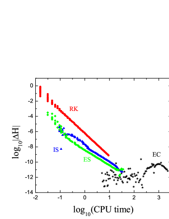
Figure 2: Efficiencies of algorithms EC, IS, ES, and RK. In fact, the efficiency describes the relation between the maximum Hamiltonian error and CPU time (unit: second) for a given step size. Each orbit has the same initial conditions, where $q_{i}=(6-i)/10$ and $p_{i}=(6-i)/100$, $\varepsilon_{m}=\varepsilon=0$, and $\beta=1$. The maximum error is obtained after the integration time $t=10^{4}$. The time steps are fixed for each algorithm, but the points correspond to different time steps $h=0.05/1.07226722^{k-1}$, where $k=1,2,\cdots,100$. Shorter CPU times correspond to larger step sizes, and longer CPU times correspond to smaller step sizes. Although EC has the poorest efficiency, its accuracy does not depend on the choice of step sizes.

Owing to its use of many iterations, EC naturally has the poorest efficiency, as shown in Figure 2. Some details with regard to drawing the efficiency plot are taken from Rein $\&$ Tamayo (2015) or Deng et al. (2020). RK exhibits the best efficiency. The efficiency of ES is better than that of IS. In particular, EC shows the best energy accuracies, which do not seem to depend on the choice of step sizes. However, the energy accuracies depend on the choice of step sizes for IS, ES, and RK. This implies that EC can use a larger step size in order to reduce computational cost.

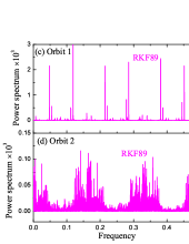
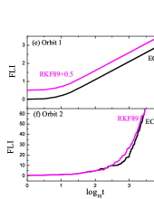
Figure 3: Power spectra and fast Lyapunov indicators (FLIs) of Orbits 1 and 2, given by methods EC and RKF89. They show that Orbit 1 is ordered, and Orbit 2 is chaotic. EC and RKF89 have the same results. Note that EC and RKF89 approximately coincide in panel (e).

The aforementioned numerical tests have confirmed that the new EC method offers long-term conservation of energy if no roundoff errors are considered. This result is independent of the dynamical behavior of the orbits. In fact, Orbit 1 is regular, but Orbit 2 is chaotic, as described by the techniques of power spectra and fast Lyapunov indicators (FLIs) in Figure 3. We make two points relating to the two techniques: the method of power spectra depicts a distribution of frequencies of orbits. In general, a regular orbit has discrete spectra, whereas a chaotic orbit exhibits continuous spectra (Wang $\&$ Wu 2011; Mei et al. 2013b). Using the two different spectra, we can roughly identify the regularity of Orbit 1, and the chaoticity of Orbit 2, which are consistently supported by the FLIs obtained from EC and RKF89 in Figures 3(a)-(d). Although the distinction between the ordered and chaotic cases can be clearly observed, the word “roughly” is still used, because complicated periodic orbits, quasi-periodic orbits, and weakly chaotic orbits may have similar continuous spectra, which may also be true of some non-periodic but non-chaotic orbits. In this sense, other methods finding chaos, such as FLIs, are necessarily employed. Wu et al. (2006) defined the FLI as

$$\emph{FLI}=\log_{10}\frac{d(t)}{d(0)},$$ (20)

where d(0) and d(t) are the phase-space distances between two adjacent orbits at times 0 and t, respectively. Clearly, this describes the growth of the phase-space distance between two adjacent orbits with time $\log_{10}t$. In fact, it originates from a modified version of the FLIS of Froeschlé et al. (1997) and Froeschlé $\&$ Lega (2000), as well as a modified version of the Lyapunov exponents (Tancredi et al. 2001; Wu $\&$ Huang 2003). However, it is more convenient to use than the FLIS of Froeschlé $\&$ Lega (2000), and is more sensitive in distinguishing between chaotic and regular bounded orbits than the technique based on Lyapunov exponents. It grows algebraically with time for the regular case, but exponentially in the chaotic case. The completely different time rates for the growth of the phase-space distance between two adjacent orbits can be used to distinguish chaos from order. The FLIs in Figures 3(e) and (f) clearly determine the properties of Orbits 1 and 2.

In short, the new EC method exhibits good performance in a long-term numerical integration. It can provide reliable numerical results, as RKF89 can. Therefore, it is employed to investigate the orbital dynamics of the DDNLS system.

3.3 Dependence of chaos on parameters

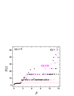
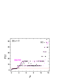
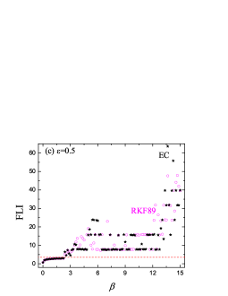
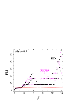
Figure 4: Dependence of FLIs on parameter $\beta$. Each orbit has the same initial variables, $q_{i}=(6-i)/10$ and $p_{i}=(6-i)/100$. Given a value of parameter $\beta$, the FLI is obtained after the integration time $t=3800$. A value of $5$ represents the threshold for FLIs, between ordered and chaotic cases. FLI$>$5 indicates the chaoticity, and FLI$\leq$5 indicates the regularity. Both EC and RKF89 give the same results.

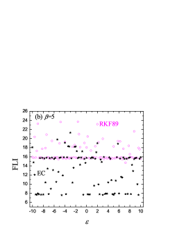
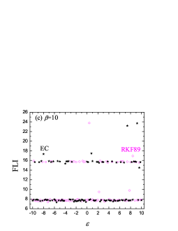
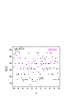
Figure 5: As Figure 4, but relating to the dependence of FLIs on parameters $\varepsilon_{m}=\varepsilon$.

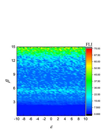
Figure 6: Finding chaos by employing FLIs to scan a two-dimensional space with parameters $\beta$ and $\varepsilon$ in the DDNLS system.

Next, let us trace the dynamical transition from order to chaos with a variation of the parameter $\beta$, or $\varepsilon_{m}=\varepsilon$. The above initial conditions are fixed, and the values of $\varepsilon$ are also given in several values, $\pm 0.5$ and $\pm 5$. However, $\beta$ runs from 0.01 to 15, with a span of $\Delta\beta=0.1499$. The FLI is obtained for each value of $\beta$ after the integration time reaches 3800. It is found that a value of 5 represents the threshold of FLIs between the ordered and chaotic cases. FLI$>$5 corresponds to the presence of chaos, and FLI$\leq$5 indicates the existence of order. Figure 4 plots the dependence of FLI on $\beta$. Chaos is absent for $\beta<2.4084$. However, it is present for $\beta>2.4084$, and the intensity of the chaos increases with an increase in $\beta$. These results are consistent with those given in Figure 5, which depict the dependence of FLI on $\varepsilon$ with fixed values of $\beta$. This is also clearly shown in terms of the FLIs in a two-dimensional space for parameters $\varepsilon$ and $\beta$ in Figure 6, too. Regardless of whether $\varepsilon$ is large or small, no chaos exists for $\beta=1$, whereas chaos exists for $\beta=5,10$,and $15$. We find similar results when other initial conditions are considered. We offer the following simple explanation of the result with respect to the dependence of dynamical transition on the parameters $\beta$ or $\varepsilon$: if $\beta=0$, the system (18) has only quadratic terms, and represents a five-dimensional coupled oscillator. In this case, it is integrable and non-chaotic. This may explain why the presence or extent of chaos does not depend on $\varepsilon$. When $\beta\neq 0$, the quartic terms cause the system (18) to be non-integrable, and probably chaotic. If $\beta$ is very small, the quadratic terms dominate the system (18), and chaos unquestionably does not occur. However, the quartic terms become more important than the quadratic terms if $\beta$ is sufficiently large. Only where the quartic terms approximately match with the quadratic terms, does chaos become possible. This further explains the data in Figures 4-6.

Several conclusions can be drawn from the numerical simulations: $\beta$ is a key parameter for inducing chaos in the DDNLS system. It has a critical value. Chaos cannot occur when $\beta$ is smaller than this critical value. Furthermore, chaos has nothing to do with the choice of parameter $\varepsilon_{m}$.

4 PN Hamiltonian of spinning compact binaries

In this section, the new EC method is applied to a PN Hamiltonian of spinning compact binaries, in order to verify whether this algorithm is still efficient. As such, the Hamiltonian is introduced in Section 4.1. Numerical estimations are given in Section 4.2. Based on the application of the EC method, the dynamics of spinning compact binaries are surveyed in Section 4.3.

4.1 PN Hamiltonian formulation

Let two black holes have masses $m_{1}$ and $m_{2}$. The total mass is $M=m_{1}+m_{2}$. Take the mass ratio $\gamma=m_{1}/m_{2}$ and the reduced mass $\mu=m_{1}m_{2}/M$. Here, $\eta=\mu/M=\gamma/(1+\gamma)^{2}$ is a dimensionless parameter; $\bm{r}=(x,y,z)$ is a position vector of the body, $m_{1}$, relative to the body, $m_{2}$, and $\bm{n}=\bm{r}/r$ is a unit radial vector. The two bodies have spins, described by $\bm{S}_{1}$ and $\bm{S}_{2}$. The speed of light, $c$, and the gravitational constant, $G$, use geometric units, $c=G=1$. Dimensionless operations are carried out via scale transformations as follows: $\bm{r}\rightarrow M\bm{r}$, $t\rightarrow Mt$, $\bm{S}_{i}\rightarrow M\mu\bm{S}_{i}$ $(i=1,2)$ and $H\rightarrow\mu H$. In addition, $\bm{p}\rightarrow\mu\bm{p}$ and $\bm{L}\rightarrow M\mu\bm{L}$, where $\bm{p}$ is a momentum of the body, $m_{1}$, relative to the body $m_{2}$, and $\bm{L}=\bm{r}\times\bm{p}$ is a Newtonian-like angular momentum vector. The evolution of $(\bm{r},\bm{p})$ is governed by the following dimensionless PN Hamiltonian formulation (Damour et al. 2000a, 2000b, 2001b; Nagar 2011):

$$H(\textbf{r},\textbf{p},\textbf{S}_{1},\textbf{S}_{2}) = H_{O}(\textbf{r},\textbf{p})+H_{SO}(\textbf{r},\textbf{p},\textbf{S}_{1},\textbf{S}_{2})$$ (21)

$$+H_{SS}(\textbf{r},\textbf{S}_{1},\textbf{S}_{2}).$$

Here, $H_{O}$ is an orbital component, including the Newtonian term and PN terms to the second order. It is written as

$$H_{O}=H_{N}(\textbf{r},\textbf{p})+H_{1PN}(\textbf{r},\textbf{p})+H_{2PN}(\textbf{r},\textbf{p}),$$ (22)

where the three sub-Hamiltonians are

$$H_{N}=\frac{\textbf{p}^{2}}{2}-\frac{1}{r},$$ (23)

$$H_{1PN} = \frac{1}{8}(3\eta-1)\textbf{p}^{4}-\frac{1}{2r}[(3+\eta)\textbf{p}^{2}$$ (24)

$$+\eta(\textbf{n}{\cdot}\textbf{p})^{2}]+\frac{1}{2r^{2}},$$

$$H_{2PN} = \frac{1}{16}(1-5\eta+5\eta{{}^{2}})\textbf{p}^{6}+\frac{1}{8r}[(5-20\eta$$ (25)

$$-3\eta^{2})\textbf{p}^{4}-2\eta^{2}(\textbf{n}\cdot\textbf{p})^{2}\textbf{p}^{2}$$

$$-3\eta^{2}(\textbf{n}\cdot\textbf{p})^{4}]+\frac{1}{2r^{2}}[(5+8\eta)\textbf{p}^{2}$$

$$+3\eta(\textbf{n}\cdot\textbf{p})^{2}]-\frac{1}{4r^{3}}(1+3\eta).$$

$H_{SO}$ is a spin-orbit coupling contribution at 1.5 PN order (Buonanno et al. 2006)

$$H_{SO}=\frac{\eta}{r^{3}}\mathbf{L}\cdot\mathbf{S}_{\mathrm{eff}},$$ (26)

where

$$\mathbf{S}_{\mathrm{eff}}=\left(2+\frac{3}{2}{}\frac{1}{\gamma}\right)\mathbf{S}_{1}+\left(2+\frac{3}{2}\gamma\right)\mathbf{S}_{2}.$$ (27)

$H_{SS}$ is a spin–spin coupling contribution at 2 PN order (Buonanno et al. 2006)

$$H_{SS}=\frac{\eta}{2r^{3}}\left[3\left(\mathbf{S}_{0}\cdot\mathbf{n}\right)^{2}-\mathbf{S}_{0}^{2}\right],$$ (28)

where

$$\mathbf{S}_{0}=(1+\frac{1}{\gamma})\mathbf{S}_{1}+(1+\gamma)\mathbf{S}_{2}.$$ (29)

Note that the Newton Wigner-Pryce spin supplementary condition $\kappa=0$ is considered (Mikóczi 2017).

The evolution of $(\bm{r},\bm{p})$ satisfies the canonical equations

$$\frac{d\mathbf{r}}{dt} = \frac{\partial H}{\partial\mathbf{p}},$$ (30)

$$\frac{d\mathbf{p}}{dt} = -\frac{\partial H}{\partial\mathbf{r}}.$$ (31)

However, the two spins vary with time, in according with non-canonical equations

$$\frac{{\rm{d}}\mathbf{S}_{i}}{{\rm{d}}t}=\frac{\partial H}{\partial\mathbf{S}_{i}}\times\mathbf{S}_{i}.$$ (32)

Equations (30)-(32) determine four integrals of motion in the system in (21). The integrals are the Hamiltonian (21) as an energy integral

$$E=H,$$ (33)

and the total angular momentum vector

$$\mathbf{J}=\mathbf{L}+\mathbf{S}_{1}+\mathbf{S}_{2}.$$ (34)

Noticing the non-canonical Equation (32), Wu $\&$ Xie (2010) introduced a pair of canonical variables $(\theta_{i},\xi_{i})$ to express each of the spins in the form

$$\mathbf{S}_{i}=\left(\begin{array}[]{c}\rho_{i}\cos\theta_{i}\\ \rho_{i}\sin\theta_{i}\\ \xi_{i}\end{array}\right),$$ (35)

where $\rho_{i}=\sqrt{\mathbf{S}_{i}^{2}-\xi_{i}^{2}}$. Clearly, $\bm{S}_{i}$ is a two-dimensional vector with three components. In this way, a ten-dimensional phase-space canonical Hamiltonian with five degrees of freedom is obtained via

$$\mathcal{H}(x,y,z,\theta_{1},\theta_{2},p_{x},p_{y},p_{z},\xi_{1},\xi_{2})$$

$$=H_{O}(x,y,z,p_{x},p_{y},p_{z})$$

$$+H_{SO}(x,y,z,\theta_{1},\theta_{2},p_{x},p_{y},p_{z},\xi_{1},\xi_{2})$$

$$+H_{SS}(x,y,z,\theta_{1},\theta_{2},\xi_{1},\xi_{2}).$$ (36)

Here, $\theta_{i}$ are generalized coordinates, and $\xi_{i}$ are conjugate momenta. These satisfy the canonical equations

$$\frac{d\theta_{i}}{dt} = \frac{\partial\mathcal{H}}{\partial\xi_{i}},$$ (37)

$$\frac{d\xi_{i}}{dt} = -\frac{\partial\mathcal{H}}{\partial\theta_{i}}.$$ (38)

The EC method is also available for Equations (30), (31), (37) and (38).

4.2 Numerical tests

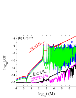
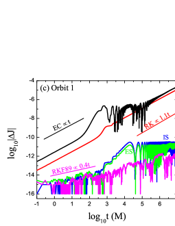
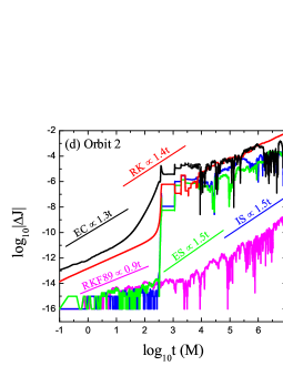
Figure 7: Hamiltonian errors, $\Delta H$, for the four algorithms solving Orbits 1 and 2 in the PN system of spinning compact binaries. The time step is $h=0.1$, and the mass ratio is $\gamma=1$. The two orbits have the initial conditions $x=40$, $y=z=p_{x}=p_{z}=0$, $p_{y}=\sqrt{(1-e)/x}$, $\theta_{1}=\theta_{2}=\pi/4$, and $\xi_{1}=\xi_{2}=0.1$. The initial eccentricities are $e=0.0985$ for Orbit 1, and $e=0.7098$ for Orbit 2. EC and RKF89 exhibit virtually the same energy errors.

In addition to the EC method, the aforementioned other algorithms RK, IS, and ES are also independently used. Letting the time step $h=0.1$, and the mass ratio $\gamma=1$, we take the initial conditions $x=40$, $y=z=p_{x}=p_{z}=0$, $p_{y}=\sqrt{(1-e)/x}$, $\theta_{1}=\theta_{2}=\pi/4$, and $\xi_{1}=\xi_{2}=0.1$, where the initial eccentricities are $e=0.0985$ for Orbit 1, and $e=0.7098$ for Orbit 2. In Figures 7 (a) and (b), the EC method almost gives the machine double-precision to the energies of Orbits 1 and 2 in an integration time of $t=1000$. When the integration spans this time, and tends to $t=10^{7}$ corresponding to $10^{8}$ steps, a slight secular drift in the energy errors occurs due to the roundoff errors. Here, EC demonstrates the best level of accuracy, as compared with the three other integrators, RK, IS, and ES. It is almost the same as the high-precision method RKF89 in terms of the magnitude of energy errors and the slope of error growth. The Hamiltonian errors for IS and ES are larger than those for EC or RKF89, but have no secular changes. Moreover, IS and ES can cause the errors of angular momentum to be bounded for Orbit 1, with a smaller eccentricity in Figure 7 (c), but to linearly grow for Orbit 2, with a larger eccentricity in Figure 7 (d). The errors of angular momentum for EC are similar to those for RK, and grow with time. This result is reasonable, because EC conserves the energy rather than the angular momentum from the theoretical viewpoint.

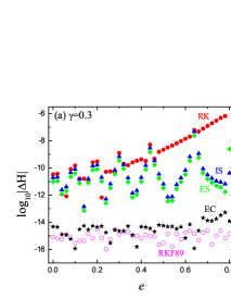
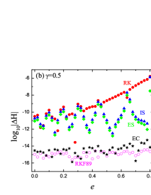
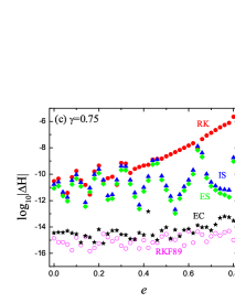
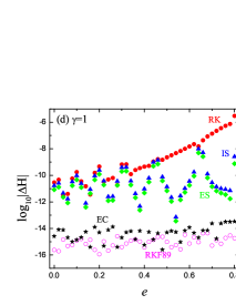
Figure 8: Relations between Hamiltonian errors $\Delta H$ for the five methods, with initial eccentricities, $e$. The same time step, $h=0.1$, is used for EC, IS, ES, and RK, but different mass ratios $\gamma$ appear in the four panels. Given a value of $e$, the error is obtained after the integration time $t=10^{5}$. The results for EC are basically consistent with those for RKF89.

It can also be seen from Figures 7 (a) and (b) that the initial eccentricities do not exert an explicit influence on the Hamiltonian errors for the EC method, unlike the three other schemes, RK, IS, and ES. To clearly show this, Figure 8 plots the dependence of the Hamiltonian errors given by the algorithms on the initial eccentricities, where several values of $\gamma$ are given. The three methods RK, IS, and ES show no dramatic differences in the Hamiltonian errors for smaller initial eccentricities. As the initial eccentricity increases, the Hamiltonian errors increase for the RK method. The IS and ES schemes result in large errors for some large initial eccentricities. However, the energy errors made by the EC method are like those made by RKF89, and are not explicitly dependent on the initial eccentricities. The numerical performance of these algorithms does not depend on the mass ratio, $\gamma$.

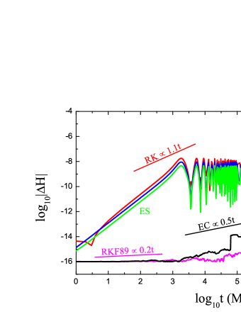
Figure 9: Hamiltonian errors, $\Delta H$, for the five algorithms solving Orbit 3 in the PN system of spinning compact binaries. The time step is $h=1$, and the mass ratio is $\gamma=1$. This orbit has the initial conditions $x=80$, $y=z=p_{x}=p_{z}=0$, and $p_{y}=\sqrt{(1-e)/x}$, where $e=0.15$, and $\theta_{1}=\theta_{2}=\xi_{1}=\xi_{2}=0$. After $10^{9}$ integration steps, IS and ES show no secular change in their energy errors. EC, like RKF89, shows a secular change in terms of energy errors, but exhibits smaller energy errors than either IS or ES.

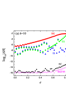
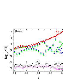
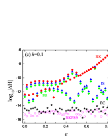
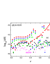
Figure 10: Figure 8 continued. The same mass ratio, $\gamma=1$, is used, but different time steps, $h$, are given.

When we take a larger step size, such as $h=1$, in Figure 9, EC, like RKF89, exhibits good accuracy up to an integration of $10^{9}$ steps, although this leads to a secular drift in the energy errors. The errors of IS and ES remain bounded, but are several orders of magnitude larger than those of EC. The accuracy of EC for the larger step size in Figure 9 is similar to that for the smaller step size in Figure 7, i.e., it is independent of the selected step size. However, the accuracy of IS, ES, and RK is closely related to the selected step size. Figure 10 provides further information regarding the dependence of algorithmic accuracy on the initial eccentricities for different choices of step size, h. It is once again clear that the energy accuracies of EC and RKF89 are not sensitive to or dependent on the choice of step sizes, unlike those of IS, ES, and RK.

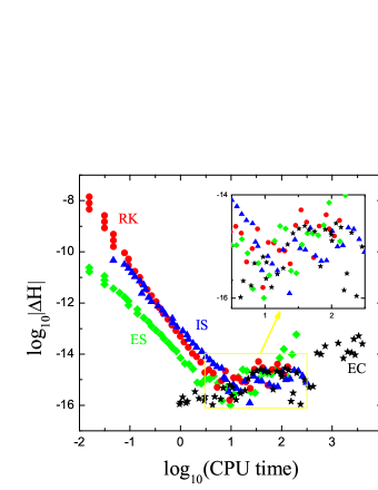
Figure 11: As Figure 2, but with the initial conditions $x=150$, $y=z=p_{x}=p_{z}=0$, $p_{y}=0.082745147$, and $\theta_{1}=\theta_{2}=\xi_{1}=\xi_{2}=0$. The maximum error is obtained after the integration time $t=10^{5}$. The time steps are fixed for each algorithm, but the points correspond to different time steps, $h=10/1.20679264^{k-1}$, where $k=1,2,\cdots,50$. Although EC exhibits the poorest efficiency, its accuracy does not depend on the choice of step size.

Although EC is more time-consuming than IS, ES, and RK in Figure 11, its energy accuracy is better, regardless of whether the step size is small or large. In particular, EC is suitable for larger step sizes. Such larger step sizes not only cause EC to behave with better accuracy, since the roundoff errors are decreased, but also leads to a reduction in EC’s computational cost. As well as the use of appropriately larger step sizes, no other methods are considered to control roundoff errors in the EC method. In fact, several authors have recently been concerned with the issue of roundoff errors, e.g., Rein $\&$ Spiegel (2015), and Wisdom (2018).

Briefly, the main conclusions to be drawn from Figures 7 – 11 are that the energy conservation in the EC method is independent of mass ratio, time step, or initial eccentricity. The EC method deals with many iterative computations, and is therefore more expensive in terms of computational cost than the implicit scheme, IS. Fortunately, the application of appropriately larger time steps to the EC method does not affect computational accuracy, and is very helpful in reducing computational cost.

4.3 Chaotic dynamics

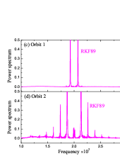
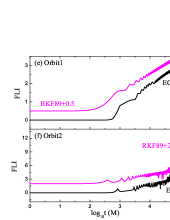
Figure 12: Power spectra and FLIs of Orbits 1 and 2 in the PN spinning binary system, obtained via the EC and RKF89 methods. Both show that Orbit 1 is ordered, and Orbit 2 is chaotic and EC and RKF89 produce the same results. Note that EC and RKF89 approximately coincide in panel (e).

In addition to the mass ratio, time step, and initial eccentricity, the dynamical feature of orbits exerts no influence on the performance of the EC method. As shown above, the EC method exhibits virtually identical errors for Orbits 1 and 2 in Figure 7. The regularity of Orbit 1, and the chaoticity of Orbit 2 are shown via the power spectra and FLIs in Figure 12.

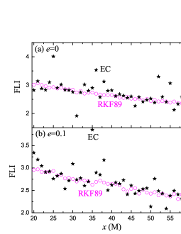
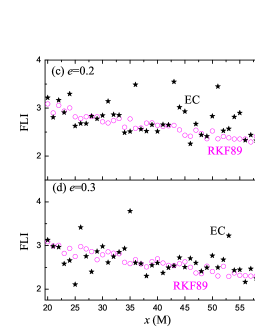
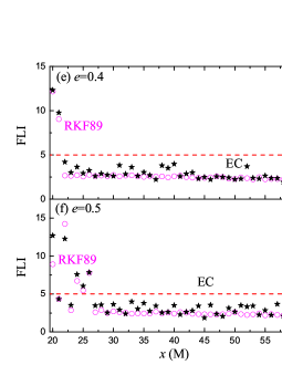
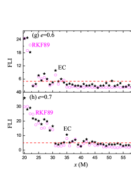
Figure 13: Relations between FLIs and initial separations, $x$. Given an initial separation $x$, the FLI is obtained after the integration time $t=3.5\times 10^{4}$. Here, FLI=5 still represents the threshold between ordered and chaotic cases. Chaos readily occurs for small initial separations and large initial eccentricities. The results for EC are the same as those for RKF89.

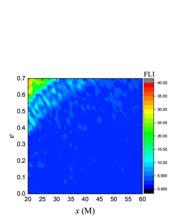
Figure 14: Finding chaos by employing FLIs to scan a two-dimensional space of initial eccentricity $e$, and initial separation, $x$, for a PN spinning binary system. The mass ratio is $\gamma=1$.

We use the EC method to discuss the relation between the chaoticity of orbits and the initial separation, $r=x$. Where the mass ratio $\gamma=1$, and the initial eccentricity $e$ is also given several values, the initial separation, $x$, runs from 20 to 60 in an interval of 1. The FLI is obtained for a given initial separation after the integration time $t=3.5\times 10^{4}$. FLI=5 is still represents the threshold between the ordered and chaotic cases. The dependence of FLIs on the initial separations, $x$, for different initial eccentricities, $e$, is plotted in Figure 13. An important result is that chaos occurs easily for smaller initial separations with higher initial eccentricities. These results can be observed quite clearly from the $x$–$e$ plane, colored in different values of FLIs in Figure 14, and are consistent with those of Hartl $\&$ Buonanno (2005). In fact, the occurrence of chaos is completely due to the spin–spin coupling contribution in Equation (28). If the spin–spin coupling is dropped, the system (21) is integrable and non-chaotic. When it is included, the system (21) is non-integrable, and then chaos becomes possible. For the case of smaller initial separations and higher initial eccentricities, the spin–spin coupling effects become larger. This is more likely to give rise to the occurrence of chaos.

In short, the EC method can provide reliable numerical results with respect to the long-term evolution of spinning compact binaries, comparable with those of the high-precision algorithm RKF89. The FLI technique is a convenient tool for finding chaos by scanning a two-dimensional space with specific parameters and initial conditions.

5 Summary

By performing a suitable discretization-averaging of the Hamiltonian canonical equations of a ten-dimensional phase-space Hamiltonian system with five degrees of freedom, in this paper, we have proposed an implicit nonsymplectic exact energy-preserving integrator. The discretization-averaging involves each component of the Hamiltonian gradient being approximately replaced with the average of ten ratios of Hamiltonian difference terms to the position or momentum increments. This approach confers a second-order accuracy on the numerical solutions.

When the new energy-conserving method is applied to a one-dimensional disordered discrete nonlinear Schrödinger equation, it exhibits good long-term numerical performance in the preservation of energy. This performance is independent of the regular and chaotic behavior of orbits. The new method can provide reliable numerical results to a problem over a long-term numerical integration, comparable to those of the high-precision algorithm RKF89. With the aid of this numerical integrator and fast Lyapunov indicators, the influence of the parameters on chaos can be studied. We have shown numerically that $\beta$, rather than $\varepsilon_{m}$, makes a significant contribution to the occurrence of chaos. No chaos can exist if $\beta$ is too small.

When the newly proposed energy-conserving integrator solves the post-Newtonian Hamiltonian system of spinning compact binaries, it still works well for long-term numerical integrations. This good long-term performance is not affected by the mass ratio, time step, initial eccentricity, or the regular/chaotic dynamical properties of orbits. Unfortunately, the new method is implicit, and therefore expensive in terms of computational cost. However, the use of appropriately large time steps makes it less time-consuming and reduces roundoff errors. The new method, combined with the technique of fast Lyapunov indicators, is highly effective in identifying the dynamical transition from order to chaos when a certain parameter or initial condition is varied. The results, concluded based on a scan of the fast Lyapunov indicators in a two-dimensional space, based on initial separation and eccentricity, is as follows: a combination of small initial separations and high initial eccentricities plays an important role in inducing chaos.

When roundoff errors are neglected, the new method has a good long-term energy conservation, irrespective of time steps, eccentricities of orbits, or the regularity/chaoticity of orbits. It can provide reliable numerical results. Thus, it is worth recommending this approach in order to simulate Hamiltonian problems with a ten-dimensional phase space, if appropriately large time steps are chosen.

Appendix

Appendix A Proof of numerical solutions accurate to the order of $h^{2}$

Expanding each increment of the Hamiltonian between $q_{1(n+1)}$ and $q_{1(n)}$ in Equation (6) to second-order partial derivatives at point $(0,0,0,0,0,0,0,0,0,0)$ in according with the Taylor expansion, we rewrite Equation (6) as follows:

$$q_{1(n+1)}-q_{1(n)} = \frac{h/10}{p_{1(n+1)}-p_{1(n)}}[(H(0000010000)-H(0000000000))+(H(1000010000)$$ (A1)

$$-H(1000000000))+(H(0000110001)-H(0000100001))+(H(1100011000)$$

$$-H(1100001000))+(H(0001110011)-H(0001100011))+(H(1110011100)$$

$$-H(1110001100))+(H(0011110111)-H(0011100111))+(H(1111011110)$$

$$-H(1111001110))+(H(0111111111)-H(0111101111))+(H(1111111111)$$

$$-H(1111101111))]$$

$$= \frac{h}{10}[(\frac{\partial H}{\partial p_{1}}+\frac{1}{2}\frac{\partial^{2}H}{\partial p^{2}_{1}}\Delta p_{1})+(\frac{\partial}{\partial p_{1}}H(1000000000)+\frac{1}{2}\frac{\partial^{2}H}{\partial p^{2}_{1}}\Delta p_{1})$$

$$+(\frac{\partial}{\partial p_{1}}H(0000100001)+\frac{1}{2}\frac{\partial^{2}H}{\partial p^{2}_{1}}\Delta p_{1})+(\frac{\partial}{\partial p_{1}}H(1100001000)+\frac{1}{2}\frac{\partial^{2}H}{\partial p^{2}_{1}}\Delta p_{1})$$

$$+(\frac{\partial}{\partial p_{1}}H(0001100011)+\frac{1}{2}\frac{\partial^{2}H}{\partial p^{2}_{1}}\Delta p_{1})+(\frac{\partial}{\partial p_{1}}H(1110001100)+\frac{1}{2}\frac{\partial^{2}H}{\partial p^{2}_{1}}\Delta p_{1})$$

$$+(\frac{\partial}{\partial p_{1}}H(0011100111)+\frac{1}{2}\frac{\partial^{2}H}{\partial p^{2}_{1}}\Delta p_{1})+(\frac{\partial}{\partial p_{1}}H(1111001110)+\frac{1}{2}\frac{\partial^{2}H}{\partial p^{2}_{1}}\Delta p_{1})$$

$$+(\frac{\partial}{\partial p_{1}}H(0111101111)+\frac{1}{2}\frac{\partial^{2}H}{\partial p^{2}_{1}}\Delta p_{1})+(\frac{\partial}{\partial p_{1}}H(1111101111)+\frac{1}{2}\frac{\partial^{2}H}{\partial p^{2}_{1}}\Delta p_{1})]$$

$$= h\frac{\partial H}{\partial p_{1}}+\frac{h}{2}\frac{\partial^{2}H}{\partial p^{2}_{1}}\Delta p_{1}+\frac{h}{10}[\frac{\partial^{2}}{\partial p_{1}\partial q_{1}}\Delta q_{1}+(\frac{\partial^{2}}{\partial p_{1}\partial q_{5}}\Delta q_{5}+\frac{\partial^{2}}{\partial p_{1}\partial p_{5}}\Delta p_{5})$$

$$+(\frac{\partial^{2}}{\partial p_{1}\partial q_{1}}\Delta q_{1}+\frac{\partial^{2}}{\partial p_{1}\partial q_{2}}\Delta q_{2}+\frac{\partial^{2}}{\partial p_{1}\partial p_{2}}\Delta p_{2})$$

$$+(\frac{\partial^{2}}{\partial p_{1}\partial q_{4}}\Delta q_{4}+\frac{\partial^{2}}{\partial p_{1}\partial q_{5}}\Delta q_{5}+\frac{\partial^{2}}{\partial p_{1}\partial p_{4}}\Delta p_{4}+\frac{\partial^{2}}{\partial p_{1}\partial p_{5}}\Delta p_{5})$$

$$+(\frac{\partial^{2}}{\partial p_{1}\partial q_{1}}\Delta q_{1}+\frac{\partial^{2}}{\partial p_{1}\partial q_{2}}\Delta q_{2}+\frac{\partial^{2}}{\partial p_{1}\partial q_{3}}\Delta q_{3}+\frac{\partial^{2}}{\partial p_{1}\partial p_{2}}\Delta p_{2}+\frac{\partial^{2}}{\partial p_{1}\partial p_{3}}\Delta p_{3})$$

$$+(\frac{\partial^{2}}{\partial p_{1}\partial q_{3}}\Delta q_{3}+\frac{\partial^{2}}{\partial p_{1}\partial q_{4}}\Delta q_{4}+\frac{\partial^{2}}{\partial p_{1}\partial q_{5}}\Delta q_{5}+\frac{\partial^{2}}{\partial p_{1}\partial p_{3}}\Delta p_{3}+\frac{\partial^{2}}{\partial p_{1}\partial p_{4}}\Delta p_{4}+\frac{\partial^{2}}{\partial p_{1}\partial p_{5}}\Delta p_{5})$$

$$+(\frac{\partial^{2}}{\partial p_{1}\partial q_{1}}\Delta q_{1}+\frac{\partial^{2}}{\partial p_{1}\partial q_{2}}\Delta q_{2}+\frac{\partial^{2}}{\partial p_{1}\partial q_{3}}\Delta q_{3}+\frac{\partial^{2}}{\partial p_{1}\partial q_{4}}\Delta q_{4}+\frac{\partial^{2}}{\partial p_{1}\partial p_{2}}\Delta p_{2}+\frac{\partial^{2}}{\partial p_{1}\partial p_{3}}\Delta p_{3}$$

$$+\frac{\partial^{2}}{\partial p_{1}\partial p_{4}}\Delta p_{4})+(\frac{\partial^{2}}{\partial p_{1}\partial q_{2}}\Delta q_{2}+\frac{\partial^{2}}{\partial p_{1}\partial q_{3}}\Delta q_{3}+\frac{\partial^{2}}{\partial p_{1}\partial q_{4}}\Delta q_{4}+\frac{\partial^{2}}{\partial p_{1}\partial q_{5}}\Delta q_{5}+\frac{\partial^{2}}{\partial p_{1}\partial p_{2}}\Delta p_{2}$$

$$+\frac{\partial^{2}}{\partial p_{1}\partial p_{3}}\Delta p_{3}+\frac{\partial^{2}}{\partial p_{1}\partial p_{4}}\Delta p_{4}+\frac{\partial^{2}}{\partial p_{1}\partial p_{5}}\Delta p_{5})+(\frac{\partial^{2}}{\partial p_{1}\partial q_{1}}\Delta q_{1}+\frac{\partial^{2}}{\partial p_{1}\partial q_{2}}\Delta q_{2}+\frac{\partial^{2}}{\partial p_{1}\partial q_{3}}\Delta q_{3}$$

$$+\frac{\partial^{2}}{\partial p_{1}\partial q_{4}}\Delta q_{4}+\frac{\partial^{2}}{\partial p_{1}\partial q_{5}}\Delta q_{5}+\frac{\partial^{2}}{\partial p_{1}\partial p_{2}}\Delta p_{2}+\frac{\partial^{2}}{\partial p_{1}\partial p_{3}}\Delta p_{3}+\frac{\partial^{2}}{\partial p_{1}\partial p_{4}}\Delta p_{4}+\frac{\partial^{2}}{\partial p_{1}\partial p_{5}}\Delta p_{5})]H$$

$$= h\frac{\partial H}{\partial p_{1}}+\frac{h}{2}\frac{\partial}{\partial p_{1}}\sum^{5}_{j=1}(\frac{\partial}{\partial q_{j}}\Delta q_{j}+{\partial p_{j}}\Delta p_{j})H+\mathcal{O}(h^{3}),$$

where $H=H(0000000000)$, and the position and momentum increments are $\Delta q_{j}=q_{j(n+1)}-q_{j(n)}$ and $\Delta p_{j}=p_{j(n+1)}-p_{j(n)}$ on the right-hand side of the above equation. In a similar way, the other position and momentum increments, including the position increment of $q_{1}$, are expressed as

$$\Delta q_{i} = h\frac{\partial}{\partial p_{i}}H(0000000000)+\frac{h}{2}\frac{\partial}{\partial p_{i}}\sum^{5}_{j=1}(\frac{\partial}{\partial q_{j}}\Delta q_{j}+{\partial p_{j}}\Delta p_{j})H(0000000000)+\mathcal{O}(h^{3}),$$ (A2)

$$\Delta p_{i} = -h\frac{\partial}{\partial q_{i}}H(0000000000)-\frac{h}{2}\frac{\partial}{\partial q_{i}}\sum^{5}_{j=1}(\frac{\partial}{\partial q_{j}}\Delta q_{j}+{\partial p_{j}}\Delta p_{j})H(0000000000)+\mathcal{O}(h^{3}),$$ (A3)

where $i=1,\cdots,5$. The position and momentum increments on the right-hand sides of Equations (A2) and (A3) take the first terms

$$\Delta q_{j} \approx h\frac{\partial}{\partial p_{i}}H(0000000000)\sim\mathcal{O}(h),$$ (A4)

$$\Delta p_{j} \approx -h\frac{\partial}{\partial q_{i}}H(0000000000)\sim\mathcal{O}(h).$$ (A5)

Substituting Equations (A4) and (A5) into Equations (A2) and (A3), we obtain the numerical solutions

$$RK: q_{i(n+1)}=p_{i(n)}+h\frac{\partial}{\partial p_{i}}H(0000000000)+\frac{h}{2}\frac{\partial}{\partial p_{i}}\sum^{5}_{j=1}(\frac{\partial}{\partial q_{j}}\Delta q_{j}+{\partial p_{j}}\Delta p_{j})H(0000000000)+\mathcal{O}(h^{3}),$$ (A7)

$$p_{i(n+1)}=p_{i(n)}-h\frac{\partial}{\partial q_{i}}H(0000000000)-\frac{h}{2}\frac{\partial}{\partial q_{i}}\sum^{5}_{j=1}(\frac{\partial}{\partial q_{j}}\Delta q_{j}+{\partial p_{j}}\Delta p_{j})H(0000000000)+\mathcal{O}(h^{3}).$$

It is clear that the numerical solutions are accurate to the order of $h^{2}$.

In fact, the numerical solutions (A6) and (A7) are those given by the refined Euler method, i.e., the second-order Runge-Kutta (RK) method. They are also obtained from the second-order implicit trapezoidal formula

$$TR: q_{i(n+1)}=q_{i(n)}+\frac{h}{2}(\frac{\partial}{\partial p_{i}}H(0000000000)+\frac{\partial}{\partial p_{i}}H(1111111111)),$$ (A9)

$$p_{i(n+1)}=p_{i(n)}-\frac{h}{2}(\frac{\partial}{\partial q_{i}}H(0000000000)+\frac{\partial}{\partial q_{i}}H(1111111111)),$$

or the second-order implicit midpoint rule (Feng 1986; Zhong et al. 2010; Mei et al. 2013a)

$$IS: q_{i(n+1)}=q_{i(n)}+h\frac{\partial}{\partial p_{i}}H(\frac{0+1}{2}\frac{0+1}{2}\frac{0+1}{2}\frac{0+1}{2}\frac{0+1}{2}\frac{0+1}{2}\frac{0+1}{2}\frac{0+1}{2}\frac{0+1}{2}\frac{0+1}{2}),$$ (A11)

$$p_{i(n+1)}=p_{i(n)}-h\frac{\partial}{\partial q_{i}}H(\frac{0+1}{2}\frac{0+1}{2}\frac{0+1}{2}\frac{0+1}{2}\frac{0+1}{2}\frac{0+1}{2}\frac{0+1}{2}\frac{0+1}{2}\frac{0+1}{2}\frac{0+1}{2}),$$

where the solutions $q_{i(n+1)}$ and $p_{i(n+1)}$ in the Hamiltonians $H(1111111111)$ and $H(\frac{0+1}{2}\cdots)$ take the first and second terms on the right-hand side of Equations (A6) and (A7), and $H(1111111111)$ and $H(\frac{0+1}{2}\cdots)$ are expanded to the order of $h$. Although the four algorithms, including the new method in Equations (6)-(15) for RK, TR, and IS, have the same order, they are different in terms of numerical performance. RK does not conserve the energy integral. IS is symplectic, and shows no secular drift in energy errors. TR is the same as IS when it is used to solve a linear Hamiltonian system, but is not symplectic for a nonlinear Hamiltonian system (Feng $\&$ Qin 2009). The new method in Equations (6)-(15) is exactly energy-conserving, theoretically, and moreover, is not symplectic.

References

- Abbott et al. (2016) Abbott, B, P., Abbott, R., Abbott, T, D., et al. 2016, Phys. Rev. Lett., 116, 061102
- Abbott et al. (2020a) Abbott, B, P., Abbott, R., Abbott, T, D., et al. 2020a, Astrophys. J. Lett., 892, L3
- Abbott et al. (2020b) Abbott, R., Abbott, T, D., Abraham, S., et al. 2020b, Phys. Rev. Lett., 125, 101102
- Bacchini et al. (2018) Bacchini, F., Ripperda, B., Chen, A, Y., et al. 2018, Astropys. J. Suppl., 237, 6 (arXiv 1801. 02378 [gr-pc])
- Bacchini et al. (2019) Bacchini, F., Ripperda, B., Chen, A, Y., et al. 2019, Astropys. J. Suppl., 240, 40 (arXiv 1810. 00842 [astro-ph.HE])
- Blanchet et al. (1995) Blanchet, L., Damour, T., Iyer, B, R. 1995, Phys. Rew. D., 51, 5360
- Blanchet et al. (2014) Blanchet, L. 2014, Living. Rew. Relativ., 17, 2
- Buonanno et al. (2006) Buonanno, A., Chen, Y., Damour, T. 2006, Phys. Rev. D., 74, 104005
- Buonanno Damour (1999) Buonanno, A., Damour, T. 1999, Phys. Rew. D., 59, 084006
- Chorin et al. (1978) Chorin, A., Huges, T, J, R., Marsden, J, E., et al. 1978, Comm. Pure and Appl. Math., 31, 205
- Cornish Levin (2002) Cornish, N, J., Levin, J. 2002, Phys. Rev. Lett., 89, 179001
- Cornish Levin (2003) Cornish, N, J., Levin, J. 2003, Phys. Rew. D., 68, 024004
- Damour et al. (2000a) Damour, T., Jaranowski, P., Schäfer, G. 2000a, Phys. Rev. D., 62, 084011
- Damour et al. (2000b) Damour, T., Jaranowski, P., Schäfer, G. 2000b, Phys. Rev. D., 62, 044024
- Damour et al. (2001a) Damour, T., Jaranowski, P., Schäfer, G. 2001a, Phys. Rew. D., 63, 044021
- Damour et al. (2001b) Damour, T., Jaranowski, P., Schäfer, G. 2001b, Phys. Lett. B., 513, 147
- de Andrade et al. (2001) de Andrade V. C., Blanchet L., Faye G. 2001, Classical Quant. Grav., 18, 753
- Deng et al. (2020) Deng, C., Wu, X., Liang, E. 2020, MNRAS, 496, 2946
- Feng (1985) Feng, K. 1985, On difference schemes and symplectic geometry. In K. Feng, editor, Proceedings of the 1984 Beijing Symposium on Differential Geometry and Differential Equations, pages 42-58 (Science Press, Beijing China)
- Feng (1986) Feng, K. 1986, J. Comput. Math., 4, 279
- Feng Qin (2009) Feng, K., Qin, M. Z. 2009, Symplectic Geometric Algorithms for Hamiltonian Systems (Zhejiang Science and Technology Publishing House, Hangzhou China, Springer, New York)
- Froeschlé et al. (1997) Froeschlé, C., Lega, E., Gonczi, R. 1997, Celest. Mech. Dyn. Astron., 67, 41
- Froeschlé Lega (2000) Froeschlé, C., Lega, E. 2000, Celest. Mech. Dyn. Astron., 78, 167
- Fukushima (2003a) Fukushima, T. 2003a, AJ, 126, 1097
- Fukushima (2003b) Fukushima, T. 2003b, AJ, 126, 2567
- Fukushima (2003c) Fukushima, T. 2003c, AJ, 126, 3138
- Fukushima (2004) Fukushima, T. 2004, AJ, 128, 3114
- Gonzalez (1996) Gonzalez, O. 1996, J. Nonlinear. Sci., 6, 449
- Gopakumar Königsdörffer (2005) Gopakumar, A., Königsdörffer, C. 2005, Phys. Rew. D., 72, 121501
- Haire et al. (2006) Hairer, E., Lubich, C., Wanner, G. 2006, GeometricNumerical Integration: Structure-Preserving Algorithms for Ordinary Differential Equations (2nd edn., Springer, Berlin)
- Harten (1983) Harten, A. 1983, J. Comput. Phys., 49, 357
- Hartl Buonanno (2005) Hartl, M, D., Buonanno, A. 2005, Phys. Rev. D., 71, 024027
- Hernandez et al. (2020) Hernandez, D, M., Hadden, S., Makino, J. 2020, MNRAS, 493, 2
- Hu et al. (2019) Hu, S, Y., Wu, X., Huang, G, Q., Liang, E. 2019, ApJ, 887, 191 (arXiv 1910. 10353 [gr-pc])
- Huang et al. (2014) Huang, G, Q., Ni, X, T., Wu, X. 2014, Eur. Phys. J. C., 74, 3012
- Huang et al. (2016) Huang, L., Wu, X., Ma, D, Z., 2016, Eur. Phys. J. C., 76, 488
- Huang Mei (2020) Huang, L., Mei, L, J. 2020, Astropys. J. Suppl., 251, 8
- Itoh Abe (1988) Itoh, T., Abe, K. 1988, J. Comp. Phys., 76, 85
- Königsdörffer Gopakumar (2005) Königsdörffer, C., Gopakumar, A. 2005, Phys. Rew. D., 71, 024039
- Levin (1999) Levin, J. 1999, Phys. Rew. D., 60, 064015
- Levin (2000) Levin, J. 2000, Phys. Rew. Lett., 84, 3515
- Levin (2003) Levin, J. 2003, Phys. Rew. D., 67, 044013
- Levin (2006) Levin, J. 2006, Phys. Rew. D., 74, 124027
- Li Wu (2017) Li, D., Wu, X. 2017, MNRAS, 469, 3031
- Li et al. (2019) Li, D., Wu, X., Liang, E, W. 2019, Ann. Phys., 531, 1900136
- Li et al. (2020) Li, D., Wang, Y., Deng, C., Wu, X. 2020, Eur. Phys. J. Plus., 135, 390
- Liao (1997) Liao, X, H. 1997, Celest. Mech. Dyn. Astr., 66, 243-253
- Liu et al. (2016) Liu, L., Wu, X., Huang, G., et al. 2016, MNRAS, 459, 1968
- Lubich (2010) Lubich, C., Walther, B., Brügmann, B. 2010, Phys. Rew. D., 81, 104025
- Luo et al. (2017) Luo, J, J., Wu, X., Huang, G, Q., et al. 2017, ApJ, 834, 64
- Ma et al. (2008a) Ma, D, Z., Wu, X., Zhong, S, Y. 2008a, ApJ, 687, 1294
- Ma et al. (2008b) Ma, D, Z., Wu, X., Zhu, J, F. 2008b, New Astron., 13, 216
- Mei et al. (2013a) Mei, L, J., Wu, X., Liu, F, Y. 2013a, Eur. Phys. J. C., 73, 2413
- Mei et al. (2013b) Mei, L, J., Ju, M, J., Wu, X., et al. 2013b, MNRAS, 435, 2246
- Mikóczi (2017) Mikóczi, B. 2017, Phys. Rev. D., 95, 064023
- Nacozy (1971) Nacozy, P, E. 1971, Astrophys. Space. Sci., 14, 40
- Nagar (2011) Nagar, A. 2011, Phys. Rew. D., 84, 084028
- Pihajoki (2015) Pihajoki, P. 2015, Celest. Mech. Dyn. Astron., 121, 211
- Preto Saha (2009) Preto, M., Saha, P. 2009, ApJ, 703, 1743
- Qin (1987) Qin, M, Z. 1987, J. Comput. Math., 5, 203
- Quispel McLaren (2008) Quispel, G, R, W., McLaren, D, I. 2008, J. Phys. A Math. Theor., 41, 045206
- Rein Tamayo (2015) Rein, H., Tamayo, D. 2015, MNRAS, 452, 376
- Rein Spiegel (2015) Rein, H., Spiegel, D, S. 2015, MNRAS, 446, 2
- Rein et al. (2019) Rein, H., Brown, G., Tamayo, D. 2019, MNRAS, 490, 4
- Robert et al. (1999) Robert, I, M., Quispel, G, R, W., Robidoux, N. 1999, Philos. T. R. Soc. A., 357, 1021
- Ruth (1983) Ruth, R, D. 1983, IEEE Trans. Nucl. Sci., NS 30, 2669
- Schnittman Rasio (2001) Schnittman, J, D., Rasio, F, A. 2001, Phys. Rev. Lett., 87, 121101
- Senyange et al. (2018) Senyange, B., Manda, B, M., Skokos, C. 2018, Phys. Rev. E., 98, 052229
- Skokos et al. (2014) Skokos, C., Gerlach, E., Bodyfelt, J, D., et al. 2014, Phys. Lett. A., 378, 1809
- Su et al. (2016) Su, X, N., Wu, X., Liu, F, Y. 2016, Astrophys. Space. Sci., 361, 32
- Tancredi et al. (2001) Tancredi, G., Sánchez, A., Roig, F. 2001, AJ, 121, 1171
- Wang et al. (2016) Wang, S, C., Wu, X., Liu, F, Y. 2016, MNRAS, 463, 1352
- Wang et al. (2018) Wang, S, C., Huang, G, Q., Wu, X. 2018, AJ, 155, 67
- Wang Wu (2011) Wang, Y., Wu, X. 2011, Commun. Theor. Phys., 56, 1045
- Wang et al. (2021a) Wang, Y., Sun, W., Liu, F, Y., Wu, X. 2021a, ApJ (Paper I), 907, 66
- Wang et al. (2021b) Wang, Y., Sun, W., Liu, F, Y., Wu, X. 2021b, ApJ (Paper II), 909, 22
- Wisdom (1982) Wisdom, J. 1982, AJ, 87, 577
- Wisdom Holman (1991) Wisdom, J., Holman, M. 1991, AJ, 102, 1528
- Wisdom (2018) Wisdom, J. 2018, MNRAS, 474, 3
- Wu Huang (2003) Wu, X., Huang, T, Y. 2003, Phys. Lett. A., 313, 77
- Wu et al. (2006) Wu, X., Huang, T., Zhang, H. 2006, Phys. Rew. D., 74, 083001
- Wu et al. (2007) Wu, X., Huang, T, Y., Wan, X, S., et al. 2007, AJ, 133, 2643
- Wu Xie (2007) Wu, X., Xie, Y. 2007, Phys. Rev. D., 76, 124004
- Wu Xie (2008) Wu, X., Xie, Y. 2008, Phys. Rev. D., 77, 103012
- Wu Xie (2010) Wu, X., Xie, Y. 2010, Phys. Rew. D., 81, 084045
- Wu et al. (2015) Wu, X., Mei, L, J., Huang, G, Q., et al. 2015, Phys. Rew. D., 91, 024042
- Wu Huang (2015) Wu, X., Huang, G, Q. 2015, MNRAS, 452, 3167
- Zhong Wu (2010) Zhong, S, Y., Wu, X. 2010, Phys. Rev. D., 81, 104037
- Zhong et al. (2010) Zhong, S, Y., Wu, X., Liu, S, Q., et al. 2010, Phys. Rev. D., 82, 124040