SUPPORTING INFORMATION FOR: Imaging properties of large field-of-view quadratic metalenses and their applications to fingerprint detection

These authors made equal contributions to this work. These authors made equal contributions to this work. These authors made equal contributions to this work. These authors made equal contributions to this work.

Number of pages: 16
Number of figures: 10
Number of tables: 1

1 Aberration analysis

Zernike polynomials compose a complete orthogonal set on a unit circular aperture to decompose the wavefront of light. Such a wavefront decomposition is particularly useful to offer a clear insight into the nature of the aberrations of an optical system. Theoretical and experimental metalens aberration analysis and comparison with traditional lenses has been done in several works ^{1, 2, 3}, however, mainly for lenses with hyperbolic phase profiles.

Here, we use the least squares method from Ref. ⁴ to decompose the wavefront of metalenses with quadratic phase profiles, allowing for fast and boundary stable calculations with orthonormal basis even on noncircular apertures. The numerically simulated wavefront of the quadratic metalens was referenced to the perfect spherical wavefront originating from the point source, numerically determined as the maximum intensity of the point spread function (PSF). The decomposition analysis was performed for two cases: metalens with a diameter $D=4f$ and $D=500\,\mu$m, both with a focal distance of $f=203\,\mu$m, which corresponds to our numerically simulated and experimentally fabricated metalenses. As shown in the main text, the effective working area of the quadratic metalens is laterally shifted within the total metalens aperture as a function of the angle of incidence (AOI). Therefore, Zernike decomposition was performed by setting the center as the center of the effective working area.

For the first case ($D=4f$), the Zernike analysis for various AOI ($\theta_{\text{i}}=0^{\circ}{}$, $30^{\circ}{}$ and $50^{\circ}{}$) is shown in Fig. S1 (a). In this case, the effective working area remains uncropped, fully inside the real aperture (i.e. the physical size of the lens, see insets), and the major aberrations are spherical and defocus. Importantly, the value of low order decomposition coefficients is not affected by the AOI (at least up to an AOI of $50^{\circ}{}$ as investigated here). Hence, aberrations and focus quality remain unaffected, as observed in Fig. 1 of the main text. The spherical aberrations are clearly visible in the ray-tracing picture as shown in Fig. S2 (a), where the farther the rays are from the optical axis (OA), the closer to the lens they intersect the OA (positive spherical aberration). The results of the Zernike decomposition for the second case ($D=500\,\mu$m) are given in Fig. S1 (b) as a function of the AOI. One can see that the effective working area is cropped by the real aperture of the lens for large AOI (see insets). Hence, additional aberrations, e.g. coma and trefoil, occur. This is illustrated in Fig. S2 (b), where in addition to spherical aberrations, the coma aberrations become particularly visible at AOI $\theta_{\text{i}}=50^{\circ}{}$ (in blue). Overall, in both cases, it is the spherical aberrations that dominate, followed by defocus aberrations, and by other ones like coma aberrations when the effective area starts to be cropped.

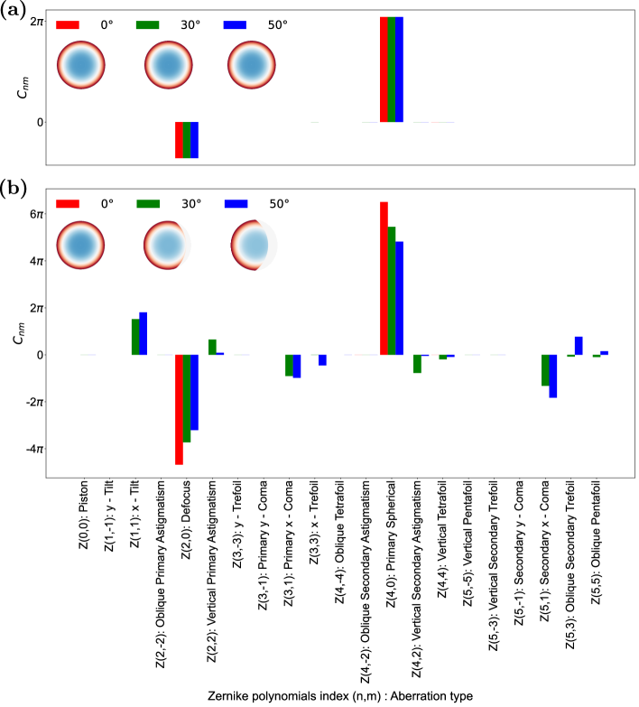
Figure S1: Zernike decomposition of the wavefront of a quadratic metalens with the focal length $f=203\,\mu$m and diameter (a) $D=4f$ and (b) $D=500\,\mu$m for three different AOI: $\theta_{\text{i}}=0^{\circ}{}$, $30^{\circ}{}$ and $50^{\circ}{}$. The insets show the corresponding wavefronts referenced to perfect spherical profiles.

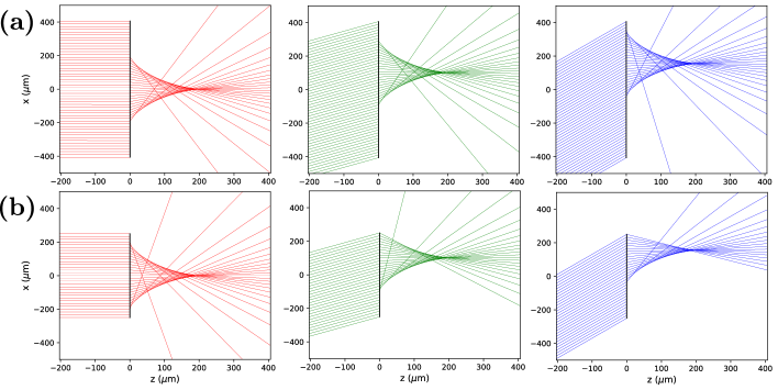
Figure S2: Ray-tracing of a quadratic metalens of focal lens $f=203\,\mu$m with diameter (a) $D=4f$ and (b) $D=500\,\mu$m for three different AOI: $\theta_{\text{i}}=0^{\circ}{}$ (in red), $30^{\circ}{}$ (in green) and $50^{\circ}{}$ (in blue). The lens lies in the plane $z=0$ (black solid line).

2 Focusing properties

Figure S3: Fourier optics simulations of the behaviour of a quadratic metalens. (a) Displacement of the focal spot in the lateral direction ($x$-direction) as a function of the AOI (green dots). The analytical formula $x(\theta_{\text{i}})=f\text{sin}(\theta_{\text{i}})$ [see Eq. (7) in the main text] is also shown (dashed black line). (b) Focusing efficiency (red dots) and FWHM of the focal spot (blue squares) as a function of the AOI. The FWHM corresponding to a diffraction-limited lens with NA$=\sqrt{2}/2$ is also shown (dashed blue line).

3 Imaging properties

In this Section, we derive the ellipse equation for the image formation using ray-tracing methods. We start by recalling the case of an ideal thin lens, in the sense of a perfect stigmatic system that images a point source into a single image point. For such a system, it is sufficient to consider two particular rays coming from an object point to obtain the corresponding image point as the intersection of these two rays in the image space. This approach is also known as the first-order ray-tracing method.

For an ideal thin lens, one uses in general two particular rays, namely, the ray passing through the center of the lens [labeled $(1)$ in Figure S4 (a)], and the ray parallel to the optical axis [labeled $(2)$ in Fig. S4 (a)]. The later will be deflected such that it passes through the focal point in the image space [labeled $(2^{\prime})$ in Fig. S4 (a)], and the former will not be deflected [labeled $(1^{\prime})$ in Fig. S4 (a)]. By considering a planar object located at a distance $d_{\text{o}}$ from the lens, and one point of this object at position $x_{\text{o}}$ (distance from optical axis), the Rays (1) and (2) in the object space are defined by the following equations in the Cartesian coordinate system ($O$,$X$, $Z$) (all quantities being taken as algebraic quantities here):

$$\text{Ray }(1): \quad x=\frac{x_{\text{o}}}{d_{\text{o}}}z$$

$$\text{Ray }(2): \quad x=-x_{\text{o}}$$

The rays in the image space are defined by the following equations:

$$\text{Ray }(1^{\prime}): \quad x=\frac{x_{\text{o}}}{d_{\text{o}}}z$$

$$\text{Ray }(2^{\prime}): \quad x=\text{tan}\left(\theta\right)z-x_{\text{o}}$$

where $\text{tan}\left(\theta\right)=x_{\text{o}}/f$. The image point is found at the intersection of Rays $(1^{\prime})$ and $(2^{\prime})$ and reads:

$$z=\frac{fd_{\text{o}}}{d_{\text{o}}-f}\;.$$ (1)

The last equation means that a planar object located at $d_{\text{o}}$ produces a planar image located at $d_{\text{i}}\equiv z=fd_{\text{o}}/(d_{\text{o}}-f)$, which is the thin lens equation usually given in the form: $1/d_{\text{o}}+1/d_{\text{i}}=1/f$ (see Fig. S4 (a)). Moreover, by combining this thin lens equation with the equation of Ray $(1^{\prime})$, one obtains the magnification: $x_{\text{i}}\equiv x=(d_{\text{i}}/d_{\text{o}})x_{\text{o}}$. One can see that the size of an image linearly depends on the object size, which is a characteristic of an ideal lens. These conclusions are in general valid for real optical systems in the paraxial approximation, that is for object points close to the OA and small AOI ($x_{\text{o}}\ll d_{\text{o}}$).

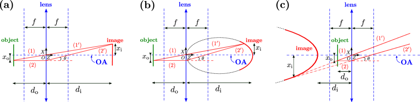
Figure S4: First-order ray-tracing for (a) an ideal and (b), (c) a quadratic lens of focal length $f$ (represented by the blue, double-arrowed line). (a) In the ideal case, the construction of the image of a planar object (green line) located at a distance $d_{\text{o}}$ from the lens is based on two special rays (red lines labeled by $(1)$, $(1^{\prime})$, $(2)$ and $(2^{\prime})$) starting from an object point $x_{\text{o}}$. Their intersection at the point $x_{\text{i}}$ gives the corresponding planar image (red line), at a distance $d_{\text{i}}$ from the lens given by Eq. (1). (b), (c) In the case of a quadratic lens, the intersection of the rays (red lines) coming from the planar object (green line) forms a curve image (red curve) which follows the equation of an ellipse given by Eq. (4) when $d_{\text{o}}>f$, or the equation of an hyperbola given by Eq. (5) when $d_{\text{o}}<f$ (dashed black lines). In configurations (a) and (b), $d_{\text{o}}=1.5f$ and $d_{\text{i}}=3f$, and in configuration (c), $d_{\text{o}}=0.6f$ and $d_{\text{i}}=1.5f$.

Now, we apply this first-order ray-tracing method to the case a quadratic metalens. For a quadratic lens, a ray parallel to the optical axis and reaching the lens at position $x$ is deflected by an angle $\theta$ which obeys: $\text{sin}\left(\theta\right)=x/f$. This means that the equation of Ray $(2^{\prime})$ must be amended by expressing $\text{tan}\left(\theta\right)$ as $\text{tan}\left(\theta\right)=\text{tan}\left[\text{arcsin}(x/f)\right]$. Moreover, using the property that $\text{tan}\left[\text{arcsin}(x/f)\right]=x/f\times 1/\sqrt{1-(x/f)^{2}}$, the equation of Ray $(2^{\prime})$ becomes:

$$\text{Ray }(2^{\prime}):\quad x=\frac{x_{\text{o}}/f}{\sqrt{1-\left(x_{\text{o}}/f\right)^{2}}}z-x_{\text{o}}$$

The image point that is found at the intersection of Rays $(1^{\prime})$ and $(2^{\prime})$ now reads:

$$z+d_{\text{o}}=\frac{d_{\text{o}}}{f}\frac{1}{\sqrt{1-\left(\frac{d_{\text{o}}}{f}\frac{x}{z}\right)^{2}}}z\;,$$ (2)

where we made used of the equation of Ray $(1^{\prime})$ to eliminate the $x_{\text{o}}$ variable and rearranged the terms. In order to derive the ellipse equation, we make the paraxial approximation, that is $x_{\text{o}}\ll d_{\text{o}}$, which implies that $x\ll z$ according to the equation of Ray $(1^{\prime})$. This allows us to make a Taylor expansion of the square-root term in Eq. (2) as:

$$\frac{1}{\sqrt{1-\left(\frac{d_{\text{o}}}{f}\frac{x}{z}\right)^{2}}}\simeq 1+\frac{1}{2}\left(\frac{d_{\text{o}}}{f}\frac{x}{z}\right)^{2}\;.$$ (3)

Thus, after some simple algebraic manipulations, Eq. (2) can be cast in the following forms, depending whether $d_{\text{o}}>f$ or $d_{\text{o}}<f$. In the case where $d_{\text{o}}>f$, the two Rays $(1^{\prime})$ and $(2^{\prime})$ intersect in the zone $z>0$ (real image) according to:

$$\frac{(z-z_{0})^{2}}{a^{2}_{\text{i}}}+\frac{x^{2}}{b^{2}_{\text{i}}}=1\quad\text{with}\quad\left\{\begin{array}[]{ll}z_{0}=\frac{1}{2}\frac{d_{\text{o}}f}{d_{\text{o}}-f}\\[5.69054pt] a_{\text{i}}=\frac{1}{2}\frac{d_{\text{o}}f}{d_{\text{o}}-f}\\[5.69054pt] b_{\text{i}}=\frac{f^{2}}{\sqrt{2d_{\text{o}}(d_{\text{o}}-f)}}\end{array}\right.\;,$$ (4)

which is the ellipse equation given in the main text (see Fig. S4 (b)). In the case where $d_{\text{o}}<f$, the two Rays $(1^{\prime})$ and $(2^{\prime})$ intersect in the zone $z<0$ (virtual image) according to:

$$\frac{(z+z_{0}^{\prime})^{2}}{a_{\text{i}}^{\prime 2}}-\frac{x^{2}}{b_{\text{i}}^{\prime 2}}=1\quad\text{with}\quad\left\{\begin{array}[]{ll}z_{0}^{\prime}=\frac{1}{2}\frac{d_{\text{o}}f}{f-d_{\text{o}}}\\[5.69054pt] a_{\text{i}}^{\prime}=\frac{1}{2}\frac{d_{\text{o}}f}{f-d_{\text{o}}}\\[5.69054pt] b_{\text{i}}^{\prime}=\frac{f^{2}}{\sqrt{2d_{\text{o}}(f-d_{\text{o}})}}\end{array}\right.\;,$$ (5)

which is the equation of a hyperbola centered on $(0,-z_{0}^{\prime})$ with transverse axis length $2a_{\text{i}}^{\prime}$ and conjugate axis length $2b_{\text{i}}^{\prime}$ (see Fig. S4 (c)).

4 Criterion for field-of-view

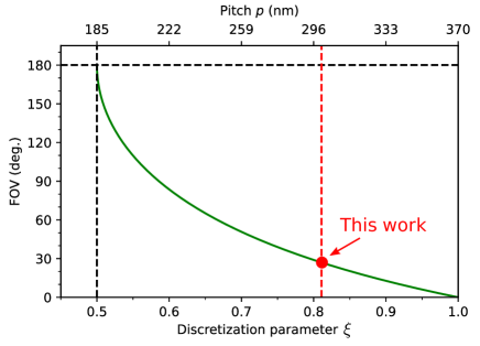
Figure S5: Minimum FOV of a quadratic metalens as given by Eq. (18) in the main text as a function of the discretization parameter $\xi$ (lower axis) and the pitch $p$ (upper axis). The later is plotted for $\lambda_{0}=740\,$nm and for the minimum unit-cell number $N=2$, which corresponds to our fabricated metalens.

5 Angle of incidence study

In addition to the simulations of the transmittance and phase as a function of the nanopillars diameters (shown in Fig. 3 (a) of the main text), we also simulated the influence of the AOI on these quantities. The results are shown in Fig. S6 as a function of the diameters and AOI, for a transverse magnetic (TM) incident wave in Fig. S6 (a) and (b), respectively, and for a transverse electric (TE) incident wave in Fig. S6 (c) and (d), respectively. One can see that the phase vary only weakly with the AOI, while the transmittance remain very high for most of the AOI and diameter parameters, except in some parameter regions where Fabry-Perot resonances occur and are responsible for strong reflections (for example, for diameters around $153\,$nm for the TE wave).

Note that we only show AOI up to $\theta_{\text{i}}=43^{\circ}{}$, which corresponds to the critical angle for an interface glass ($n=1.46$) - air ($n=1$); beyond this critical angle, the transmission efficiency is zero, due to the total internal reflection. However, this effect is a peculiarity of simulations that consider periodic arrangements of identical nanopillars, and does not occur in the metalens since the gradient of phase imparted through different nanopillars gives the required extra momentum for light to be transmitted. To show that, we also simulated the transmission efficiencies of four different phase-gradient metasurfaces made of supercells with respectively $N=9$, $6$, $3$ and $2$ nanopillars, each nanopillars being encompassed in a “unit-cell” of cross section $p\times p$ with $p=300\,$nm. Each supercell samples linearly the $2\pi$ phase by its number of element $N$ by carefully choosing the correct nanopillars (see first column in Table S1). These four supercells are representative of the ones used in the quadratic metalens. In Table S1, we show the computed transmission efficiencies (in red) for TM and TE incident waves and for three different AOI $\theta_{\text{i}}=0^{\circ}{}$, $30^{\circ}{}$ and $50^{\circ}{}$, together with the relative efficiencies into the blazed diffraction order (in blue). One can see that energy is still transmitted at $\theta_{\text{i}}=50^{\circ}{}$ (which is above the critical angle), for the reasons given above. The fact that there is no energy into the blazed order at $\theta_{\text{i}}=0^{\circ}{}$ in the case of supercells with $N=2$ elements (second column / last row in Table S1) is because such a surpercell is sub-diffractive at normal incidence (its length $Np<\lambda_{0}$ with $\lambda_{0}=740\,$nm). Note, however, that for the AOI $\theta_{\text{i}}=30^{\circ}{}$ and $50^{\circ}{}$ the first-order (blazed) diffraction channel becomes propagating and the supercell becomes “active”. In particular, for certain configurations of polarizations and AOI, only the channel corresponding to the blazed order is available, and therefore this channel has 100% of relative efficiency (see Table S1).

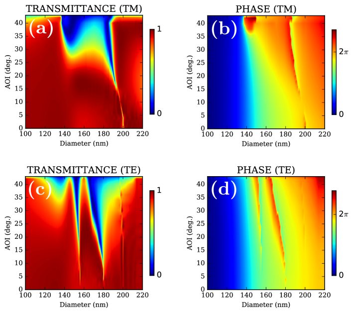
Figure S6: Transmission efficiencies (transmittances) and phases of a periodic arrangement of identical nanopillars as a function of their diameters and AOI. (a), (b) Case of a TM incident wave. (c), (d) Case of a TE incident wave.

$N$	$0^{\circ}{}$ (TM / TE)	$30^{\circ}{}$ (TM / TE)	$50^{\circ}{}$ (TM / TE)
	$97\%$ / $94\%$	$59\%$ / $82\%$	$28\%$ / $40\%$
	$95\%$ / $98\%$	$37\%$ / $55\%$	$86\%$ / $28\%$
	$92\%$ / $94\%$	$56\%$ / $80\%$	$35\%$ / $44\%$
	$93\%$ / $96\%$	$44\%$ / $90\%$	$77\%$ / $31\%$
	$45\%$ / $63\%$	$73\%$ / $77\%$	$33\%$ / $26\%$
	$61\%$ / $74\%$	$67\%$ / $76\%$	$100\%$ / $71\%$
	$14\%$ / $62\%$	$67\%$ / $97\%$	$38\%$ / $59\%$
	$0\%$ / $0\%$	$70\%$ / $99\%$	$100\%$ / $100\%$

Table S1: Transmission efficiencies (in red) for different AOI $\theta_{\text{i}}=0^{\circ}{}$, $30^{\circ}{}$ and $50^{\circ}{}$ of different phase-gradient metasurfaces containing supercells with $N=9$, $6$, $3$ and $2$ elements, respectively, computed for TM and TE incident waves. The relative efficiencies into the blazed diffractive order are also shown (in blue).

6 Barrel distortion

In this Section, we derive analytical formulas to quantify the barrel distortion effect, in order to unveil the existing trade-off between the maximum FOV of an object that can be imaged and the optical resolution of the metalens and/or the detector resolution. The barrel distortion, or fish-eye effect, is the fact that equally spaced object points produce image points that get more compressed in the edges of the image. More specifically, one can show that, for an object point located at a distance $x_{\text{o}}$ from the OA (see Fig. 4 (a) in the main text), a quadratic metalens will produce an image point located at $x_{\text{i}}$:

$$x_{\text{i}}=f\,\frac{x_{\text{o}}/d}{\sqrt{1+\left(x_{\text{o}}/d\right)^{2}}}\;.$$ (6)

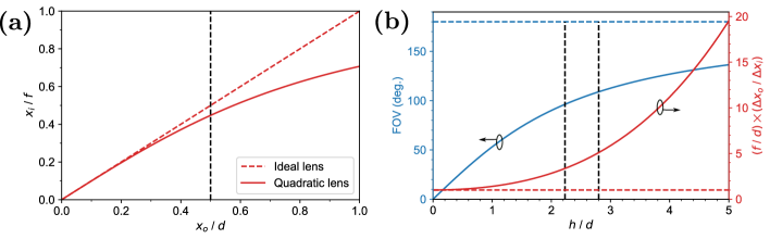
Figure S7: Barrel distortion effect. (a) Point-to-point imaging: image point $x_{\text{i}}$ normalized by $f$ as a function of the corresponding object point $x_{\text{o}}$ normalized by $d$ for a quadratic lens (solid red line). The case of an ideal lens is also shown (dashed red line). (b) Relative image resolution $\Delta x_{\text{o}}/\Delta x_{\text{i}}$ normalized by $d/f$ (solid red line) and object FOV (solid blue line) as a function of the object size $h$ normalized by $d$. The limit FOV $=180^{\circ}{}$ is also shown (dashed blue line). The relative resolution in the case of an ideal lens $\Delta x_{\text{o}}/\Delta x_{\text{i}}=d/f$ is also shown (dashed red line). The two ruler imaging configurations {$d=3\,$cm, $h=6.7\,$cm} and {$d=2\,$cm, $h=5.6\,$cm} are indicated by the two vertical dashed lines (left and right, respectively).

This behavior is shown in Fig. S7 (d), where we plot the image position given by Eq. (6) as a function of the object position (solid red line), together with the behavior of an ideal lens with no distortion (dashed red line). As seen, there is less than 10% of distortion for object points located at a distance $x_{\text{o}}<0.5d$ (this limit is shown by the vertical dashed line), which is barely visible to the naked eye. Indeed, one can check by looking at Figs. 5 (b) and (c) in the main text, that those parts of the ruler up to $h=d$, corresponding to $h=3\,$cm and $h=2\,$cm, respectively, are almost not distorted.

One can see from Eq. (6) that, as the distance of the object points $x_{\text{o}}$ increases, the distance $x_{\text{i}}$ increases at an increasingly slower pace (due to the denominator). This in turn will increase the image spatial resolution required to resolve these points. To quantify this, we start by differentiating Eq. (6) with respect to the distance $x_{\text{o}}$ to obtain:

$$\frac{\Delta x_{\text{o}}}{\Delta x_{\text{i}}}=\frac{d}{f}\left[1+\left(\frac{x_{\text{o}}}{d}\right)^{2}\right]^{3/2}\;,$$ (7)

where $\Delta x_{\text{o}}$ is the distance between two adjacent object points to be resolved, and $\Delta x_{\text{i}}$ is the distance between the corresponding image points. In practice, $\Delta x_{\text{o}}$ is the minimum object feature size that one wants to image and, depending on which one is the limiting factor, $\Delta x_{\text{i}}$ corresponds to either the detector spatial resolution, or to the optical spatial resolution of the lens. In the following, we call the ratio $\Delta x_{\text{o}}/\Delta x_{\text{i}}$ the relative image resolution. In Fig. S7 (e), we plot (solid red line) this relative image resolution $\Delta x_{\text{o}}/\Delta x_{\text{i}}$ given by Eq. (7) as a function of the object size $h$ ($x_{\text{o}}=h/2$) normalized by the distance $d$. We also show the FOV of the object given by Eq. (17) from the main text (solid blue line). One can see that, as the ratio $h/d$ increases, both the relative image resolution and FOV increase.

Finally, by using Eq. (17) from the main text into Eq. (7), we find the relation between the FOV of an object that can be resolved and the relative spatial resolution $\Delta x_{\text{o}}/\Delta x_{\text{i}}$:

$$\text{FOV}=2\,\text{arctan}\left(\sqrt{\left(\frac{f}{d}\frac{\Delta x_{\text{o}}}{\Delta x_{\text{i}}}\right)^{\frac{2}{3}}-1}\right)\;,$$ (8)

which corresponds to Eq. (18) of the main text. In other words, this equation predicts, for a given image spatial resolution $\Delta x_{\text{i}}$, what is the maximum FOV of an object with features down to $\Delta x_{\text{o}}$ in size that can be resolved (see Fig. S8 for a plot of this maximum FOV). The application of this formula to the ruler case in the configurations $d=3\,$cm and $d=2\,$cm gives, with $\Delta x_{\text{o}}\sim 1\,$mm and $\Delta x_{\text{i}}\sim 2\,\mu$m, maximum FOV of $96^{\circ}{}$ and $109^{\circ}{}$, respectively.

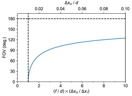
Figure S8: Maximum FOV of an object as given by Eq. (8) as a function of the relative spatial resolution normalized by $d/f$ (lower axis) and the ratio $\Delta x_{\text{o}}/d$ (upper axis). The later is plotted for $\Delta x_{\text{i}}=2\,\mu$m and $f=203\,\mu$m, which corresponds to our fabricated metalens.

7 Imaging experiment

The main text presents the imaging of the ruler and the fingerprint. Both were printed on a white paper and illuminated by the laser in a transmission configuration. Since the ruler is an elongated object, a Thorlabs $0.4^{\circ}\times 100^{\circ}$ line engineered diffuser was utilized to produce a line pattern. The image produced by the metalens was transferred to a CCD camera by a free-space microscope setup with 5X magnification (20X Nikon infinity-corrected objective, NA=0.45, a tube lens with 50 mm focal length, see Fig. S9 (a)).

As far as the fingerprint imaging is concerned, as discussed in the main text, the smallest possible object-lens distance $d=800\,\mu$m corresponds to the thickness of the metalens substrate. To demonstrate this most extreme case, we fabricated a small focal length metalens ($f=100\,\mu$m, $D=246\,\mu$m) and glued the fingerprint image on the opposite side of the substrate. The imaging result is presented in Fig. S9 (b). As one can expect, the object size one can image is quite limited due to the barrel distortions, resulting in $\sim 1.5\,\text{mm}\times 1.5\,$mm visible fingerprint area.

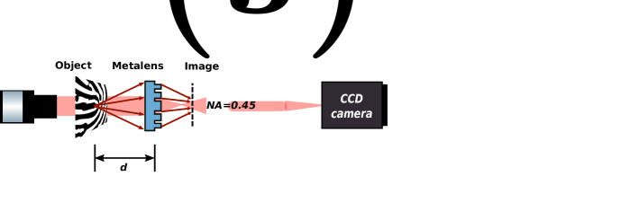
Figure S9: Imaging experiment. (a) Schematic of the optical setup. The light red color denotes the laser beam path in the absence of the object. (b) The result of the experimental imaging of the fingerprint at $d=800\,\mu$m. The scale bar corresponds to $50\,\mu$m.

8 MTF analysis

To give more insight on the quadratic lens imaging performance, we provide here a monochromatic modulation transfer function (MTF) calculation. The MTF of an optical system describes the image contrast attenuation arising from the finite resolution of the optics. Mathematically, the MTF is calculated as the normalized Fourier transform of the PSF, showing the contrast drop for each spatial frequency.

In Fig. S10 (a), we calculated the MTF at the working wavelength $\lambda_{0}=740\,$nm for on-axis ($0^{\circ}{}$ AOI, solid green line) and off-axis points ($30^{\circ}{}$ and $50^{\circ}{}$ AOI, blue and red lines, respectively) for both horizontal and vertical directions (called tangential and sagittal directions in the legend of the figure, respectively). The quadratic lens MTF is compared to a diffraction-limited system with an $\text{NA}=0.37$ (solid black line; see also main text, Section 3.2.3). One can see that the quadratic lens exhibits a rapid contrast drop down to about $10\%$ at $150$ cycles/mm (vertical dashed black line), which is mainly associated with inherent spherical aberrations discussed in the main text. One can also see that the cutoff spatial frequency (i.e., the spatial frequency above which the MTF is equal to zero), defined as $1000\times 2\text{NA}/\lambda_{0}$ (to have it in cycles/mm), is about the same for both and equal to about $1000$ cycles/mm.

To improve the contrast, an aperture stop (pinhole) located at the front focal plane of the lens can be utilized ⁵. In Fig. S10 (b), we present the MTF calculation for a pinhole-metalens system (the green and blue lines can barely be distinguished because they coincide almost perfectly). The pinhole has a diameter of $100\,\mu$m (i.e., about $f/2$). A glass substrate is taken as the medium located between the pinhole and the metalens. One can see that, while the cutoff spatial frequency in the pinhole-metalens system case is about 650 cycles/mm, due to the overall NA reduction, such an arrangement can provide a substantial improvement of the MTF, that may be beneficial for the realization of better devices.

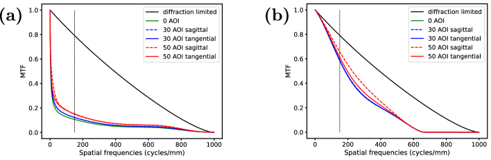
Figure S10: MTF calculations for monochromatic illumination at $\lambda_{0}=740\,$nm for two different configurations: quadratic metalens (a) without and (b) with a pinhole of diameter $100\,\mu$ located at the front focal plane of the lens. The calculations are performed for three different AOI: $0^{\circ}{}$ (green line), $30^{\circ}{}$ (blue lines) and $50^{\circ}{}$ (red lines), and for both tangential and sagittal directions. The MTF of a diffraction-limited system with an $\text{NA}=0.37$ is also shown (solid black line). The vertical black dashed line is a guide-to-the eye at $150$ cycles/mm.

References

- Decker et al. 2019 Decker, M.; Chen, W. T.; Nobis, T.; Zhu, A. Y.; Khorasaninejad, M.; Bharwani, Z.; Capasso, F.; Petschulat, J. Imaging performance of polarization-insensitive metalenses. ACS Photonics 2019, 6, 1493–1499
- Banerji et al. 2019 Banerji, S.; Meem, M.; Majumder, A.; Vasquez, F. G.; Sensale-Rodriguez, B.; Menon, R. Imaging with flat optics: metalenses or diffractive lenses? Optica 2019, 6, 805–810
- Khadir et al. 2021 Khadir, S.; Andrén, D.; Verre, R.; Song, Q.; Monneret, S.; Genevet, P.; Käll, M.; Baffou, G. Metasurface optical characterization using quadriwave lateral shearing interferometry. ACS Photonics 2021, 8, 603–613
- Dai and Mahajan 2008 Dai, G.-M.; Mahajan, V. N. Orthonormal polynomials in wavefront analysis: error analysis. Applied Optics 2008, 47, 3433–3445
- Engelberg et al. 2020 Engelberg, J.; Wildes, T.; Zhou, C.; Mazurski, N.; Bar-David, J.; Kristensen, A.; Levy, U. How good is your metalens? Experimental verification of metalens performance criterion. Optics Letters 2020, 45, 3869–3872