Thermodynamically Consistent Algorithms for Models of Diblock Copolymer Solutions Interacting with Electric and Magnetic Fields

Xiaowen Shen0.10.10.1sxw@csrc.ac.cn, Beijing Computational Science Research Center, Beijing 100193, China. , Qi Wang0.20.20.2qwang@math.sc.edu, Department of Mathematics, University of South Carolina, Columbia, SC 29208, USA.
Abstract

We derive thermodynamically consistent models for diblock copolymer solutions coupled with the electric and magnetic field, respectively. These models satisfy the second law of thermodynamics and therefore are therefore thermodynamically consistent. We then design a set of 2nd order, linear, semi-discrete schemes for the models using the energy quadratization method and the supplementary variable method, respectively, which preserve energy dissipation rates of the models. The spatial discretization is carried out subsequently using 2nd order finite difference methods, leading to fully discrete algorithms that preserve discrete energy-dissipation-rates of the models so that the resulting fully discrete models are thermodynamically consistent. Convergence rates are numerically confirmed through mesh refinement tests and several numerical examples are given to demonstrate the role of the mobility in pattern formation, defect removing effect of both electric and magnetic fields as well as the hysteresis effect for applied external fields in copolymer solutions.

Keywords: Phase field; Diblock copolymer solution; Electric field; Magnetic field; Thermodynamically consistent models.

1 Introduction

A polymer is a class of natural or synthetic substances composed of macromolecules. The block copolymer comprises of two or more homopolymer subunits linked by covalent bonds. The block copolymer solution is a mixture of copolymers and solvent. In the diblock copolymer solution, whose copolymer consists of polymer A𝐴A and polymer B𝐵B, the solvent can be water or another homopolymer that serves as a solvent for A/B𝐴𝐵A/B polymers. Diblock copolymers can self-assemble into various ordered mesoscopic structures as the result of polymer-polymer and polymer-solvent interaction, which are useful in materials science and engineering, in particular, nanotechnologies [17, 18, 19]. In experiments, copolymer solutions often undergo macroscopic phase separation between the copolymer and solvent or microscopic phase separation between polymer A𝐴A and polymer B𝐵B components. A number of meso-structures of copolymer melts and solutions have been experimentally observed and theoretically predicted via the self-consistent mean field theory as well as the phase field theory. In 2D, there are spot and lamellar morphologies; whereas in 3D cases, the class of possible stable structures is rather abundant including lamellae, spheroids, cylinders and gyrations [8, 42, 38, 22, 48, 4].

The phase field approach and associated numerical simulations have proven to be effective means to investigate dynamics in copolymer systems. The seminal work of Ohta and Kawasaki [23] laid the foundation of the phase field models for diblock copolymer system. Ohta et al. [24] also considered models for mixtures of diblock copolymers and a third immiscible phase. Choksi and Ren [9, 10] rederived the models with rigorous mathematical details. Recently, some rigorous analyses on minimizers of the free energy functional or stable steady states of the Ohta–Kawasaki model in both 2D and 3D were reported [35, 36], providing insightful information about the dynamics and their attractors in the model of copolymer systems.

Applying an external electric field or magnetic field to copolymer systems is one of the efficient ways to manipulate and produce various nanostructured materials in self-assembly involving copolymers [31, 29, 12]. The electric or magnetic field assisted self-assembly is a cutting-edge research topic in materials science and engineering today.

When the electric field is applied to a copolymer system, dipoles are induced so that the electric field is fully coupled to dynamics of the copolymer system. The existing phase field models for this problem, however, have adopted a over-simplified approach which results in a model that does not respect the thermodynamical consistency in the coupled system of equations [41, 39, 30, 28, 6, 3, 49]. In fact, all existing models coupling the electric field are based on two original papers [2, 40], where significant simplified approximations were applied. As the result, the models do not satisfy the second law of thermodynamics. This thermodynamical inconsistency prevents one from devising structure-preserving numerical approximations, which are thermodynamically consistent at the discrete level, to the important class of models for copolymer solutions with a wide range of applications in fabrications of novel materials. Thermodynamical consistency here refers to the positive entropy production principle in nonequilibrium thermodynamics expressed either as the generalized Onsager principle or as the second law of thermodynamics. It is an important principle to follow when devising mathematical models for any material systems. It is also an important criterion to respect when designing numerical algorithms.

In this paper, we will first derive a thermodynamically consistent phase field model for the diblock copolymer solution or melt system interacting with electric and magnetic fields, following fundamental principles of electrodynamics [21] and the generalized Onsager principle [44, 37]. In particular, the model for copolymer systems with coupled electric field respects the energy dissipation law, overcoming the shortcomings in the previous models for copolymer systems coupled with the electric field due to over-simplification. These thermodynamically consistent models allow us to design efficient and accurate structure-preserving numerical algorithms to simulate field assisted processing of diblock copolymer solutions based on the dynamical models while respecting the model specific energy dissipation rate.

Around 2011, Badia and Tierra et al. explored an idea of transforming the free energy into a quadratic functional to derive energy stable schemes [1, 14, 15]. Later the idea was amplified and systematically applied to many specific thermodynamic and hydrodynamic models by Yang, Zhao, Shen and Wang et al. [51, 32, 33, 5], which is termed energy quadratization. The energy quadratization (EQ) strategy bypasses the traditional complicated ones to arrive at semi-discrete, 2nd order or higher order in time linear schemes readily. This strategy is so general that it has little restriction on the specific expression of the free energy density so long as it is bounded below required by physics. Shen, Xu and Yang proposed the scalar auxiliary variable (SAV) method based upon the EQ strategy for gradient flow systems so long as their free energies are bounded below [32, 33]. In [51], Wang et al. summarized previous works they had done using the EQ strategy and presented a general framework to discretize the thermodynamically consistent models in forms of partial differential equations to arrive at linear, 2nd order, energy stable numerical schemes. Yang and Shen et al. applied the EQ and SAV strategies to copolymer melts and copolymer-homopolymer mixtures and proposed a set of energy stable schemes [6, 43, 48]. Zhang et al. used a stabilized SAV method to discretize a magnetic field coupled copolymer melt model and a hydrodynamic model to develop energy stable schemes recently [50, 4].

For a dissipative system, a numerical scheme is called energy stable if it respects energy decay. Among energy stable schemes, the ones that preserve the energy-dissipation-rate are better than the ones that simply preserve energy dissipation inequalities since the energy dissipation rate in the energy stable discrete scheme may not be calculated accurately or even correctly despite of the energy decay property in general. Usually, excessive dissipation is added to the discrete equation system to ensure energy stability. Therefore, developing numerical schemes that preserve the energy-dissipation-rate is desirable and very important. There are no numerical works that preserve energy-dissipation-rates of diblock copolymer systems on the original free energy and the corresponding energy-dissipation-rate yet.

In [13, 20], Wang et al. proposed a new temporal discretization paradigm for developing energy-production-rate preserving numerical approximations to thermodynamically consistent partial differential equations with deduced equations, called the supplementary variable method (SVM). The central idea behind this method is to introduce a set of supplementary variables to the thermodynamically consistent model to remove the over-determinedness of the system of equations consisting of the partial differential equations and the deduced equations (the energy definition and the energy-dissipation-rate equation). The introduction of supplementary variables allows one to enforce the deduced equations (i.e., the energy dissipation rate equation in the diblock copolymer model) at the discrete level as intended. This numerical paradigm can be applied to any partial differential equation systems with deduced equations including thermodynamically consistent gradient flow models as well as hydrodynamic models. Upon discretization, some implementations of this method resemble that of the Lagrange multiplier method proposed by Cheng, Liu and Shen recently [5], and they also share some similarity to the extended SAV approach discussed by Yang and Dong in [45] and the projection method in [16]. This numerical strategy allows a great degree of freedom in the implementation of the supplementary variables in the governing system of equations compared to the other methods mentioned above.

As the second component of this paper, we design a series of energy dissipation rate preserving numerical algorithms for the thermodynamically consistent, electric and magnetic fields coupled phase field model for diblock copolymer solutions, respectively. These schemes are linear, 2nd order and energy-dissipation-rate preserving based on the energy quadratization and the supplementary variable strategy, respectively. The SVM is presented as a prediction-correction scheme, in which the solution and the energy dissipation rate are predicted using 2nd order schemes in the predictive step and the solution and the energy dissipation rate are corrected within the same order to satisfy the discrete equation that respects the energy dissipation rate. The solution of the supplementary variable consumes a negligibly small computational cost, making this method quite efficient compared to the EQ method. We then use a developed scheme to numerically simulate transient dynamics of the diblock copolymer solution coupled with electric and magnetic fields.

The rest of the paper is organized as follows. In Section 2, using the Onsager principle along with the theory on electrodynamics, we derive thermodynamically consistent phase field models for the diblock copolymer solution coupled with an electric field and a magnetic field, respectively. In Section 3, we recall numerical strategies in the EQ method and SVM for gradient flow models. In Section 4, we develop a set of fully discrete, linear, 2nd order, structure-preserving schemes. In Section 5, we numerically demonstrate the accuracy and energy stability of proposed schemes. Then we use one of the SVM schemes to numerically simulate transient dynamics in the copolymer solution system driven by electric and magnetic fields. In Section 6, we give some concluding remarks.

2 Thermodynamically consistent models

We derive the thermodynamically consistent models for the diblock copolymer solution that couples the electric and magnetic fields properly. We begin the derivation with a brief review of the generalized Onsager principle which is a constructive method for developing thermodynamically consistent models.

2.1 Onsager principle

Nonequilibrium phenomena require models derived from principles of nonequilibrium thermodynamics to describe. The generalized Onsager principle is a linear response theory for developing dynamical models for nonequilibrium phenomena near the equilibrium of any matter systems [25, 26, 27, 44, 37]. Assuming the thermodynamical variables describing nonequilibrium phenomena of the matter system are denoted as ϕ(𝒙,t)Nbold-italic-ϕ𝒙𝑡superscript𝑁\bm{\phi}(\bm{x},t)\in\mathbb{R}^{N}, where N𝑁N is the number of the variables, and the free energy of the matter system is prescribed by a functional F[ϕ]𝐹delimited-[]bold-italic-ϕF[\bm{\phi}] in isothermal cases (for nonisothermal cases, we would have to use an entropy functional instead). The Onsager linear response theory states

𝑹ϕ˙=𝑴𝝁,𝝁=δFδϕ,formulae-sequence𝑹˙bold-italic-ϕ𝑴𝝁𝝁𝛿𝐹𝛿bold-italic-ϕ\bm{R}\dot{\bm{\phi}}=-\bm{M}\bm{\mu},\quad\bm{\mu}=\frac{\delta F}{\delta\bm{\phi}}, (2.1)

where 𝑹𝑹\bm{R} and 𝑴𝑴\bm{M} are operators, 𝑴1𝑹superscript𝑴1𝑹\bm{M}^{-1}\bm{R} is known as the friction and 𝑹1𝑴superscript𝑹1𝑴\bm{R}^{-1}\bm{M} as the mobility operator (or matrix) when they exist. This equation system provides relaxation dynamics for the nonequilibrium state to return to equilibrium in dissipative systems or to oscillate in nondissipative systems. Without loss of generality, we assume 𝑹=I𝑹𝐼\bm{R}=I in this work so that 𝑴𝑴\bm{M} is the mobility operator.

In general, the mobility operator 𝑴(ϕ)𝑴bold-italic-ϕ\bm{M}(\bm{\phi}) can be decomposed into a symmetric part 𝑴s(ϕ)subscript𝑴𝑠bold-italic-ϕ\bm{M}_{s}(\bm{\phi}), satisfying the reciprocal relation [25, 26], and an antisymmetric part 𝑴a(ϕ)subscript𝑴𝑎bold-italic-ϕ\bm{M}_{a}(\bm{\phi}) as follows

𝑴=𝑴a+𝑴s.𝑴subscript𝑴𝑎subscript𝑴𝑠\bm{M}=\bm{M}_{a}+\bm{M}_{s}. (2.2)

The time rate of change of the free energy is given by

dFdt=ΩδFδϕ𝑴δFδϕ𝑑𝒙=ΩδFδϕ𝑴sδFδϕ𝑑𝒙,𝑑𝐹𝑑𝑡subscriptΩ𝛿𝐹𝛿bold-italic-ϕ𝑴𝛿𝐹𝛿bold-italic-ϕdifferential-d𝒙subscriptΩ𝛿𝐹𝛿bold-italic-ϕsubscript𝑴𝑠𝛿𝐹𝛿bold-italic-ϕdifferential-d𝒙\frac{dF}{dt}=-\int_{\Omega}\frac{\delta F}{\delta\bm{\phi}}\bm{M}\frac{\delta F}{\delta\bm{\phi}}d\bm{x}=-\int_{\Omega}\frac{\delta F}{\delta\bm{\phi}}\bm{M}_{s}\frac{\delta F}{\delta\bm{\phi}}d\bm{x}, (2.3)

under proper adiabatic boundary conditions on ϕbold-italic-ϕ\bm{\phi}. Here, ΩΩ\Omega is the domain that the system occupies. If 𝑴s0subscript𝑴𝑠0\bm{M}_{s}\geq 0 is positive semi-definite, the system is a dissipative system; if 𝑴s=0subscript𝑴𝑠0\bm{M}_{s}=0, it is a conservative one.

2.2 Free energy

We adopt a free energy functional firstly derived by Ohta et al. [24] and then reformulated by Choksi and Ren [10]. Consider the diblock copolymer solution in a fixed domain Ωd(d=2,3)Ωsuperscript𝑑𝑑23\Omega\subset\mathbb{R}^{d}(d=2,3). We utilize Nisubscript𝑁𝑖{N_{i}} to denote the polymerization degree of species i=A,B,S𝑖𝐴𝐵𝑆i=A,B,S (NS=1subscript𝑁𝑆1N_{S}=1 when the solvent is water). We denote the local volume fraction of each component as ϕi(𝒙,t),i=A,B,S,formulae-sequencesubscriptitalic-ϕ𝑖𝒙𝑡𝑖𝐴𝐵𝑆\phi_{i}(\bm{x},t),i=A,B,S, respectively. In the following, we use either i=A,B,S𝑖𝐴𝐵𝑆i=A,B,S or i=1,2,3𝑖123i=1,2,3, or even omit them in some cases for convenience. The free energy functional consists of 2 parts

F=FS+FL,𝐹subscript𝐹𝑆subscript𝐹𝐿F=F_{S}+F_{L}, (2.4)

where FS,FLsubscript𝐹𝑆subscript𝐹𝐿F_{S},F_{L} represent the short and long range energy, respectively. The short range part FSsubscript𝐹𝑆F_{S} is given by

FS=Ω[iγi2|ϕi|2+i,jχij2ϕiϕj+f(ϕ)]𝑑𝒙,f(ϕ)=iϕiNilnϕi,formulae-sequencesubscript𝐹𝑆subscriptΩdelimited-[]subscript𝑖subscript𝛾𝑖2superscriptsubscriptitalic-ϕ𝑖2subscript𝑖𝑗subscript𝜒𝑖𝑗2subscriptitalic-ϕ𝑖subscriptitalic-ϕ𝑗𝑓bold-italic-ϕdifferential-d𝒙𝑓bold-italic-ϕsubscript𝑖subscriptitalic-ϕ𝑖subscript𝑁𝑖subscriptitalic-ϕ𝑖F_{S}=\int_{\Omega}\Big{[}\sum_{i}\frac{\gamma_{i}}{2}|\nabla\phi_{i}|^{2}+\sum_{i,j}\frac{\chi_{ij}}{2}\phi_{i}\phi_{j}+f(\bm{\phi})\Big{]}d\bm{x},\quad f(\bm{\phi})=\sum_{i}\frac{\phi_{i}}{N_{i}}\ln\phi_{i}, (2.5)

where χij(=χji)annotatedsubscript𝜒𝑖𝑗absentsubscript𝜒𝑗𝑖\chi_{ij}(=\chi_{ji}) is the interaction constant between polymer i𝑖i and polymer j𝑗j (χii=0subscript𝜒𝑖𝑖0\chi_{ii}=0). The long range part FLsubscript𝐹𝐿F_{L} is given by

FL=i,jαij2ΩΩG(𝒙,𝒚)[ϕi(𝒙)ϕ¯i][ϕj(𝒚)ϕ¯j]𝑑𝒚𝑑𝒙,subscript𝐹𝐿subscript𝑖𝑗subscript𝛼𝑖𝑗2subscriptΩsubscriptΩ𝐺𝒙𝒚delimited-[]subscriptitalic-ϕ𝑖𝒙subscript¯italic-ϕ𝑖delimited-[]subscriptitalic-ϕ𝑗𝒚subscript¯italic-ϕ𝑗differential-d𝒚differential-d𝒙F_{L}=\sum_{i,j}\frac{\alpha_{ij}}{2}\int_{\Omega}\int_{\Omega}G(\bm{x},\bm{y})[\phi_{i}(\bm{x})-\overline{\phi}_{i}][\phi_{j}(\bm{y})-\overline{\phi}_{j}]d\bm{y}d\bm{x}, (2.6)

where

ϕ¯i=1|Ω|Ωϕi(𝒙)𝑑𝒙,i=A,B,S,formulae-sequencesubscript¯italic-ϕ𝑖1ΩsubscriptΩsubscriptitalic-ϕ𝑖𝒙differential-d𝒙𝑖𝐴𝐵𝑆\overline{\phi}_{i}=\frac{1}{|\Omega|}\int_{\Omega}\phi_{i}(\bm{x})~{}d\bm{x},\quad i=A,B,S, (2.7)

G𝐺G is the Green’s function with homogeneous Neumann boundary conditions such that

Δ𝒚G(𝒙,𝒚)=δ(𝒙𝒚)inΩ,subscriptΔ𝒚𝐺𝒙𝒚𝛿𝒙𝒚inΩ-\Delta_{\bm{y}}G(\bm{x},\bm{y})=\delta(\bm{x}-\bm{y})\quad{\rm in}~{}\Omega, (2.8)

δ(𝒙𝒚)𝛿𝒙𝒚\delta(\bm{x}-\bm{y}) denotes the Dirac measure giving unit mass to the point 𝒙𝒙\bm{x}, and αijsubscript𝛼𝑖𝑗\alpha_{ij} are the coupling constants, γisubscript𝛾𝑖\gamma_{i} measure the strength of the conformational entropy. The Kuhn length of the copolymer is set to unity. In the reformulation of Choksi and Ren [10], parameters of the model admit the following relations

γi=ε2ϕ¯i,(αij)=32εγ[1/(ϕ¯Aϕ¯A)1/(ϕ¯Aϕ¯B)01/(ϕ¯Aϕ¯B)1/(ϕ¯Bϕ¯B)0000].formulae-sequencesubscript𝛾𝑖superscript𝜀2subscript¯italic-ϕ𝑖subscript𝛼𝑖𝑗32𝜀𝛾delimited-[]matrix1subscript¯italic-ϕ𝐴subscript¯italic-ϕ𝐴1subscript¯italic-ϕ𝐴subscript¯italic-ϕ𝐵01subscript¯italic-ϕ𝐴subscript¯italic-ϕ𝐵1subscript¯italic-ϕ𝐵subscript¯italic-ϕ𝐵0000\gamma_{i}=\frac{\varepsilon^{2}}{\overline{\phi}_{i}},\quad(\alpha_{ij})=\frac{3}{2}\varepsilon\gamma\left[\begin{matrix}1/(\overline{\phi}_{A}\overline{\phi}_{A})&-1/(\overline{\phi}_{A}\overline{\phi}_{B})&0\\ -1/(\overline{\phi}_{A}\overline{\phi}_{B})&1/(\overline{\phi}_{B}\overline{\phi}_{B})&0\\ 0&0&0\end{matrix}\right]. (2.9)

We define

ψj(𝒙):=ΩG(𝒙,𝒚)[ϕj(𝒚)ϕ¯j]𝑑𝒚Δψj=ϕjϕ¯j,formulae-sequenceassignsubscript𝜓𝑗𝒙subscriptΩ𝐺𝒙𝒚delimited-[]subscriptitalic-ϕ𝑗𝒚subscript¯italic-ϕ𝑗differential-d𝒚Δsubscript𝜓𝑗subscriptitalic-ϕ𝑗subscript¯italic-ϕ𝑗\psi_{j}(\bm{x}):=-\int_{\Omega}G(\bm{x},\bm{y})[\phi_{j}(\bm{y})-\overline{\phi}_{j}]d\bm{y}\quad\Leftrightarrow\quad\Delta\psi_{j}=\phi_{j}-\overline{\phi}_{j}, (2.10)

with Neumann boundary conditions ψj𝒏|Ω=0,j=A,B,Sformulae-sequenceevaluated-atsubscript𝜓𝑗𝒏Ω0𝑗𝐴𝐵𝑆\nabla\psi_{j}\cdot\bm{n}|_{\partial\Omega}=0,~{}j=A,B,S. Then, we obtain an equivalent free energy

F[ϕ]=Ω[iγi2|ϕi|2+i,jχij2ϕiϕj+f(ϕ)]𝑑𝒙i,jαij2Ω[ϕi(𝒙)ϕ¯i]ψj(𝒙)𝑑𝒙.𝐹delimited-[]bold-italic-ϕsubscriptΩdelimited-[]subscript𝑖subscript𝛾𝑖2superscriptsubscriptitalic-ϕ𝑖2subscript𝑖𝑗subscript𝜒𝑖𝑗2subscriptitalic-ϕ𝑖subscriptitalic-ϕ𝑗𝑓bold-italic-ϕdifferential-d𝒙subscript𝑖𝑗subscript𝛼𝑖𝑗2subscriptΩdelimited-[]subscriptitalic-ϕ𝑖𝒙subscript¯italic-ϕ𝑖subscript𝜓𝑗𝒙differential-d𝒙F[\bm{\phi}]=\int_{\Omega}\Big{[}\sum_{i}\frac{\gamma_{i}}{2}|\nabla\phi_{i}|^{2}+\sum_{i,j}\frac{\chi_{ij}}{2}\phi_{i}\phi_{j}+f(\bm{\phi})\Big{]}d\bm{x}-\sum_{i,j}\frac{\alpha_{ij}}{2}\int_{\Omega}[\phi_{i}(\bm{x})-\overline{\phi}_{i}]\psi_{j}(\bm{x})d\bm{x}. (2.11)

2.3 Thermodynamically consistent diblock copolymer solution model

The time rate of change of the free energy given above is calculated as follows

dFdt=Ωi(γiΔϕi+jχijϕj+fϕi)ϕitd𝒙+Ωiγiϕi𝒏ϕitdsi,jαijΩψjϕit𝑑𝒙.𝑑𝐹𝑑𝑡subscriptΩsubscript𝑖subscript𝛾𝑖Δsubscriptitalic-ϕ𝑖subscript𝑗subscript𝜒𝑖𝑗subscriptitalic-ϕ𝑗𝑓subscriptitalic-ϕ𝑖subscriptitalic-ϕ𝑖𝑡𝑑𝒙subscriptΩsubscript𝑖subscript𝛾𝑖subscriptitalic-ϕ𝑖𝒏subscriptitalic-ϕ𝑖𝑡𝑑𝑠subscript𝑖𝑗subscript𝛼𝑖𝑗subscriptΩsubscript𝜓𝑗subscriptitalic-ϕ𝑖𝑡differential-d𝒙\frac{dF}{dt}=\int_{\Omega}\sum_{i}\Big{(}-\gamma_{i}\Delta\phi_{i}+\sum_{j}\chi_{ij}\phi_{j}+\frac{\partial f}{\partial\phi_{i}}\Big{)}\frac{\partial\phi_{i}}{\partial t}d\bm{x}+\int_{\partial\Omega}\sum_{i}\gamma_{i}\nabla\phi_{i}\cdot\bm{n}\frac{\partial\phi_{i}}{\partial t}ds-\sum_{i,j}\alpha_{ij}\int_{\Omega}\psi_{j}\frac{\partial\phi_{i}}{\partial t}d\bm{x}. (2.12)

In the adiabatic case, the surface energy dissipation vanishes at the zero Neumann boundary conditions:

ϕi𝒏|Ω=0,i=A,B,S.formulae-sequenceevaluated-atsubscriptitalic-ϕ𝑖𝒏Ω0𝑖𝐴𝐵𝑆\nabla\phi_{i}\cdot\bm{n}|_{\partial\Omega}=0,\quad i=A,B,S. (2.13)

The chemical potentials are given by

μAsubscript𝜇𝐴\displaystyle\mu_{A} =δFδϕA=γAΔϕA+jχAjϕj+fϕAαAAψAαABψB,absent𝛿𝐹𝛿subscriptitalic-ϕ𝐴subscript𝛾𝐴Δsubscriptitalic-ϕ𝐴subscript𝑗subscript𝜒𝐴𝑗subscriptitalic-ϕ𝑗𝑓subscriptitalic-ϕ𝐴subscript𝛼𝐴𝐴subscript𝜓𝐴subscript𝛼𝐴𝐵subscript𝜓𝐵\displaystyle=\frac{\delta F}{\delta\phi_{A}}=-\gamma_{A}\Delta\phi_{A}+\sum_{j}\chi_{Aj}\phi_{j}+\frac{\partial f}{\partial\phi_{A}}-\alpha_{AA}\psi_{A}-\alpha_{AB}\psi_{B}, (2.14)
μBsubscript𝜇𝐵\displaystyle\mu_{B} =δFδϕB=γBΔϕB+jχBjϕj+fϕBαABψAαBBψB,absent𝛿𝐹𝛿subscriptitalic-ϕ𝐵subscript𝛾𝐵Δsubscriptitalic-ϕ𝐵subscript𝑗subscript𝜒𝐵𝑗subscriptitalic-ϕ𝑗𝑓subscriptitalic-ϕ𝐵subscript𝛼𝐴𝐵subscript𝜓𝐴subscript𝛼𝐵𝐵subscript𝜓𝐵\displaystyle=\frac{\delta F}{\delta\phi_{B}}=-\gamma_{B}\Delta\phi_{B}+\sum_{j}\chi_{Bj}\phi_{j}+\frac{\partial f}{\partial\phi_{B}}-\alpha_{AB}\psi_{A}-\alpha_{BB}\psi_{B},
μSsubscript𝜇𝑆\displaystyle\mu_{S} =δFδϕS=γSΔϕS+jχSjϕj+fϕS.absent𝛿𝐹𝛿subscriptitalic-ϕ𝑆subscript𝛾𝑆Δsubscriptitalic-ϕ𝑆subscript𝑗subscript𝜒𝑆𝑗subscriptitalic-ϕ𝑗𝑓subscriptitalic-ϕ𝑆\displaystyle=\frac{\delta F}{\delta\phi_{S}}=-\gamma_{S}\Delta\phi_{S}+\sum_{j}\chi_{Sj}\phi_{j}+\frac{\partial f}{\partial\phi_{S}}.

Now we derive the transport equations for the copolymer solution system using the Onsager principle. The transport equations are proposed as

ϕit=ji,i=A,B,S,formulae-sequencesubscriptitalic-ϕ𝑖𝑡subscript𝑗𝑖𝑖𝐴𝐵𝑆\frac{\partial\phi_{i}}{\partial t}=j_{i},\quad i=A,B,S, (2.15)

where jisubscript𝑗𝑖j_{i} is the rate of production for ϕi,i=A,B,Sformulae-sequencesubscriptitalic-ϕ𝑖𝑖𝐴𝐵𝑆\phi_{i},i=A,B,S, respectively. We add the incompressibility condition to the free energy as a constraint through Lagrange multiplier L𝐿L:

E[ϕ,L]=F[ϕ]+ΩL(𝒙,t)(ϕA+ϕB+ϕS1)𝑑𝒙.𝐸bold-italic-ϕ𝐿𝐹delimited-[]bold-italic-ϕsubscriptΩ𝐿𝒙𝑡subscriptitalic-ϕ𝐴subscriptitalic-ϕ𝐵subscriptitalic-ϕ𝑆1differential-d𝒙E[\bm{\phi},L]=F[\bm{\phi}]+\int_{\Omega}L(\bm{x},t)(\phi_{A}+\phi_{B}+\phi_{S}-1)d\bm{x}. (2.16)

The time derivative of the free energy becomes

dEdt=Ω[(μA+L)ϕAt+(μB+L)ϕBt+(μS+L)ϕSt]𝑑𝒙.𝑑𝐸𝑑𝑡subscriptΩdelimited-[]subscript𝜇𝐴𝐿subscriptitalic-ϕ𝐴𝑡subscript𝜇𝐵𝐿subscriptitalic-ϕ𝐵𝑡subscript𝜇𝑆𝐿subscriptitalic-ϕ𝑆𝑡differential-d𝒙\frac{dE}{dt}=\int_{\Omega}\Big{[}(\mu_{A}+L)\frac{\partial\phi_{A}}{\partial t}+(\mu_{B}+L)\frac{\partial\phi_{B}}{\partial t}+(\mu_{S}+L)\frac{\partial\phi_{S}}{\partial t}\Big{]}d\bm{x}. (2.17)

We apply the Onsager principle to obtain

[jA,jB,jS]=𝑴[μA+L,μB+L,μS+L],superscriptsubscript𝑗𝐴subscript𝑗𝐵subscript𝑗𝑆top𝑴superscriptsubscript𝜇𝐴𝐿subscript𝜇𝐵𝐿subscript𝜇𝑆𝐿top[j_{A},j_{B},j_{S}]^{\top}=-\bm{M}[\mu_{A}+L,\mu_{B}+L,\mu_{S}+L]^{\top}, (2.18)

where

𝑴=(M)=([M11(ϕ)M12(ϕ)M13(ϕ)M12(ϕ)M22(ϕ)M23(ϕ)M13(ϕ)M23(ϕ)M33(ϕ)])𝑴𝑀delimited-[]matrixsubscript𝑀11bold-italic-ϕsubscript𝑀12bold-italic-ϕsubscript𝑀13bold-italic-ϕsubscript𝑀12bold-italic-ϕsubscript𝑀22bold-italic-ϕsubscript𝑀23bold-italic-ϕsubscript𝑀13bold-italic-ϕsubscript𝑀23bold-italic-ϕsubscript𝑀33bold-italic-ϕ\bm{M}=-\nabla\cdot(M\nabla)=-\nabla\cdot\Big{(}\left[\begin{matrix}M_{11}(\bm{\phi})&M_{12}(\bm{\phi})&M_{13}(\bm{\phi})\\ M_{12}(\bm{\phi})&M_{22}(\bm{\phi})&M_{23}(\bm{\phi})\\ M_{13}(\bm{\phi})&M_{23}(\bm{\phi})&M_{33}(\bm{\phi})\end{matrix}\right]\nabla\Big{)} (2.19)

is the mobility operator and Mijsubscript𝑀𝑖𝑗M_{ij} are the coefficients. So the dynamical equations are given as follows

{ΔψA=ϕAϕ¯A,ΔψB=ϕBϕ¯B,ϕAt=[M11(μA+L)]+[M12(μB+L)]+[M13(μS+L)],ϕBt=[M12(μA+L)]+[M22(μB+L)]+[M23(μS+L)],ϕSt=[M13(μA+L)]+[M23(μB+L)]+[M33(μS+L)],(i,jMijL)=(i,jMijμi).\left\{\begin{aligned} &\Delta\psi_{A}=\phi_{A}-\overline{\phi}_{A},\quad\Delta\psi_{B}=\phi_{B}-\overline{\phi}_{B},\\ &\frac{\partial\phi_{A}}{\partial t}=\nabla\cdot\big{[}M_{11}\nabla(\mu_{A}+L)\big{]}+\nabla\cdot\big{[}M_{12}\nabla(\mu_{B}+L)\big{]}+\nabla\cdot\big{[}M_{13}\nabla(\mu_{S}+L)\big{]},\\ &\frac{\partial\phi_{B}}{\partial t}=\nabla\cdot\big{[}M_{12}\nabla(\mu_{A}+L)\big{]}+\nabla\cdot\big{[}M_{22}\nabla(\mu_{B}+L)\big{]}+\nabla\cdot\big{[}M_{23}\nabla(\mu_{S}+L)\big{]},\\ &\frac{\partial\phi_{S}}{\partial t}=\nabla\cdot\big{[}M_{13}\nabla(\mu_{A}+L)\big{]}+\nabla\cdot\big{[}M_{23}\nabla(\mu_{B}+L)\big{]}+\nabla\cdot\big{[}M_{33}\nabla(\mu_{S}+L)\big{]},\\ &\nabla\cdot\Big{(}\sum_{i,j}M_{ij}\nabla L\Big{)}=-\nabla\cdot\Big{(}\sum_{i,j}M_{ij}\nabla\mu_{i}\Big{)}.\end{aligned}\right. (2.20)

The adiabatic boundary conditions for the copolymer model are

𝒏M[μA+L,μB+L,μS+L]|Ω=𝟎,𝒏ϕi|Ω=0,i=A,B,S,ψj𝒏|Ω=0,j=A,B.\bm{n}\cdot M\cdot\nabla[\mu_{A}+L,\mu_{B}+L,\mu_{S}+L]^{\top}\big{|}_{\partial\Omega}=\bm{0},~{}\bm{n}\cdot\nabla\phi_{i}|_{\partial\Omega}=0,i=A,B,S,~{}\nabla\psi_{j}\cdot\bm{n}|_{\partial\Omega}=0,j=A,B. (2.21)

Under these boundary conditions, we obtain the energy dissipation rate

dEdt=Ω[μA+L,μB+L,μS+L]M[μA+L,μB+L,μS+L]𝑑𝒙.𝑑𝐸𝑑𝑡subscriptΩsubscript𝜇𝐴𝐿subscript𝜇𝐵𝐿subscript𝜇𝑆𝐿𝑀subscript𝜇𝐴𝐿subscript𝜇𝐵𝐿subscript𝜇𝑆𝐿differential-d𝒙\frac{dE}{dt}=-\int_{\Omega}\nabla[\mu_{A}+L,\mu_{B}+L,\mu_{S}+L]\cdot M\cdot\nabla[\mu_{A}+L,\mu_{B}+L,\mu_{S}+L]d\bm{x}. (2.22)

The model is energy dissipative provided (Mij)0subscript𝑀𝑖𝑗0(M_{ij})\geq 0. We note that the Onsager principle also allows one to propose nonadiabatic boundary conditions in which energy can exchange with the surrounding. For simplicity, we focus on the adiabatic case in this study.

2.4 Electric field coupled model

Copolymers are responsive to external field such as electric and magnetic fields. Field assisted processing is one of the promising means to control the morphology of the copolymer system. The electric and magnetic fields impact on the copolymer system by modifying the free energy landscape. Developing a thermodynamically consistent relaxation model for the copolymer system subject to external fields is an important first step in understanding dynamics of the system. Finding stable steady state (or low energy state) along with the energy decaying path is of great importance [7, 34, 46, 47]. In this paper, we utilize the PDE paradigm to describe the dynamical path, whose governing equations are derived from the Onsager principle. This is one legitimate description of relaxation dynamics from the nonequilibrium state to return to the equilibrium state through the mobility operator.

We consider the additional free energy due to the existence of electric field 𝑬𝑬\bm{E}

Fe=Ω12𝑫𝑬𝑑𝒙=Ω12ϵ𝑫𝑫𝑑𝒙,subscript𝐹esubscriptΩ12𝑫𝑬differential-d𝒙subscriptΩ12italic-ϵ𝑫𝑫differential-d𝒙F_{\rm e}=\int_{\Omega}\frac{1}{2}\bm{D}\cdot\bm{E}~{}d\bm{x}=\int_{\Omega}\frac{1}{2\epsilon}\bm{D}\cdot\bm{D}~{}d\bm{x}, (2.23)

where 𝑫=ϵ𝑬𝑫italic-ϵ𝑬\bm{D}=\epsilon\bm{E} is the electric displacement, ϵitalic-ϵ\epsilon is the dielectric constant, which can be approximated as [2, 40]

ϵ(𝒙,t)=ϵ0+ϵ1φ,φ=(ϕAϕB)(ϕ¯Aϕ¯B),formulae-sequenceitalic-ϵ𝒙𝑡subscriptitalic-ϵ0subscriptitalic-ϵ1𝜑𝜑subscriptitalic-ϕ𝐴subscriptitalic-ϕ𝐵subscript¯italic-ϕ𝐴subscript¯italic-ϕ𝐵\epsilon(\bm{x},t)=\epsilon_{0}+\epsilon_{1}\varphi,\quad\varphi=(\phi_{A}-\phi_{B})-(\overline{\phi}_{A}-\overline{\phi}_{B}), (2.24)

where ϵ0subscriptitalic-ϵ0\epsilon_{0} is the vacuum permittivity, ϵ1subscriptitalic-ϵ1\epsilon_{1} is a constant related to the material. Because of the inhomogeneity of ϵ(𝒙,t)italic-ϵ𝒙𝑡\epsilon(\bm{x},t), the electric field 𝑬𝑬\bm{E} inside the material deviates from the applied electric field 𝑬0subscript𝑬0\bm{E}_{0} and is given by

𝑬=𝑬0Φ,𝑬subscript𝑬0Φ\bm{E}=\bm{E}_{0}-\nabla\Phi, (2.25)

where ΦΦ\Phi is the electric potential for the induced electric field. ΦΦ\Phi can be expressed in terms of φ𝜑\varphi or ϕbold-italic-ϕ\bm{\phi}, by solving the following Poisson equation (Gauss theorem)

𝑫=[(ϵ0+ϵ1φ)(𝑬0Φ)]=ϵ0ΔΦ+ϵ1𝑬0φϵ1φΦϵ1φΔΦ=0,𝑫delimited-[]subscriptitalic-ϵ0subscriptitalic-ϵ1𝜑subscript𝑬0Φsubscriptitalic-ϵ0ΔΦsubscriptitalic-ϵ1subscript𝑬0𝜑subscriptitalic-ϵ1𝜑Φsubscriptitalic-ϵ1𝜑ΔΦ0\nabla\cdot\bm{D}=\nabla\cdot\big{[}(\epsilon_{0}+\epsilon_{1}\varphi)(\bm{E}_{0}-\nabla\Phi)\big{]}=-\epsilon_{0}\Delta\Phi+\epsilon_{1}\bm{E}_{0}\cdot\nabla\varphi-\epsilon_{1}\nabla\varphi\cdot\nabla\Phi-\epsilon_{1}\varphi\Delta\Phi=0, (2.26)

where we use the Dirichlet boundary condition Φ|Ω=Φ0evaluated-atΦΩsubscriptΦ0\Phi|_{\partial\Omega}=\Phi_{0} for the electric potential and Φ0subscriptΦ0\Phi_{0} is a prescribed value (we use Φ0=0subscriptΦ00\Phi_{0}=0 in this study).

Following the work of [21], we have

dFedt=Ω12ϵ2|𝑫|2ϵφφtd𝒙=Ωϵ12|𝑬|2(ϕAtϕBt)d𝒙.𝑑subscript𝐹e𝑑𝑡subscriptΩ12superscriptitalic-ϵ2superscript𝑫2italic-ϵ𝜑𝜑𝑡𝑑𝒙subscriptΩsubscriptitalic-ϵ12superscript𝑬2subscriptitalic-ϕ𝐴𝑡subscriptitalic-ϕ𝐵𝑡𝑑𝒙\frac{dF_{\rm e}}{dt}=\int_{\Omega}-\frac{1}{2\epsilon^{2}}|\bm{D}|^{2}\frac{\partial\epsilon}{\partial\varphi}\frac{\partial\varphi}{\partial t}d\bm{x}=\int_{\Omega}-\frac{\epsilon_{1}}{2}|\bm{E}|^{2}\Big{(}\frac{\partial\phi_{A}}{\partial t}-\frac{\partial\phi_{B}}{\partial t}\Big{)}d\bm{x}. (2.27)

Since the total free energy is given by

E[ϕ,L]=F[ϕ]+Fe[ϕ]+ΩL(𝒙,t)(ϕA+ϕB+ϕS1)𝑑𝒙.𝐸bold-italic-ϕ𝐿𝐹delimited-[]bold-italic-ϕsubscript𝐹edelimited-[]bold-italic-ϕsubscriptΩ𝐿𝒙𝑡subscriptitalic-ϕ𝐴subscriptitalic-ϕ𝐵subscriptitalic-ϕ𝑆1differential-d𝒙E[\bm{\phi},L]=F[\bm{\phi}]+F_{\rm e}[\bm{\phi}]+\int_{\Omega}L(\bm{x},t)(\phi_{A}+\phi_{B}+\phi_{S}-1)d\bm{x}. (2.28)

the time derivative of the total free energy becomes

dEdt=Ω[(μA+μe+L)ϕAt+(μBμe+L)ϕBt+(μS+L)ϕSt]𝑑𝒙,μe=ϵ12|𝑬0Φ|2.formulae-sequence𝑑𝐸𝑑𝑡subscriptΩdelimited-[]subscript𝜇𝐴subscript𝜇e𝐿subscriptitalic-ϕ𝐴𝑡subscript𝜇𝐵subscript𝜇e𝐿subscriptitalic-ϕ𝐵𝑡subscript𝜇𝑆𝐿subscriptitalic-ϕ𝑆𝑡differential-d𝒙subscript𝜇esubscriptitalic-ϵ12superscriptsubscript𝑬0Φ2\frac{dE}{dt}=\int_{\Omega}\Big{[}(\mu_{A}+\mu_{\rm e}+L)\frac{\partial\phi_{A}}{\partial t}+(\mu_{B}-\mu_{\rm e}+L)\frac{\partial\phi_{B}}{\partial t}+(\mu_{S}+L)\frac{\partial\phi_{S}}{\partial t}\Big{]}d\bm{x},~{}\mu_{\rm e}=-\frac{\epsilon_{1}}{2}|\bm{E}_{0}-\nabla\Phi|^{2}. (2.29)

We denote μ^A=μA+μe,μ^B=μBμe,μ^S=μSformulae-sequencesubscript^𝜇𝐴subscript𝜇𝐴subscript𝜇eformulae-sequencesubscript^𝜇𝐵subscript𝜇𝐵subscript𝜇esubscript^𝜇𝑆subscript𝜇𝑆\widehat{\mu}_{A}=\mu_{A}+\mu_{\rm e},~{}\widehat{\mu}_{B}=\mu_{B}-\mu_{\rm e},~{}\widehat{\mu}_{S}=\mu_{S}. Using the Onsager principle, we obtain the model coupled with the electric field

{ΔψA=ϕAϕ¯A,ΔψB=ϕBϕ¯B,[(ϵ0+ϵ1φ)(𝑬0Φ)]=0,ϕAt=[M11(μ^A+L)]+[M12(μ^B+L)]+[M13(μ^S+L)],ϕBt=[M12(μ^A+L)]+[M22(μ^B+L)]+[M23(μ^S+L)],ϕSt=[M13(μ^A+L)]+[M23(μ^B+L)]+[M33(μ^S+L)],(i,jMijL)=(i,jMijμ^i).\left\{\begin{aligned} &\Delta\psi_{A}=\phi_{A}-\overline{\phi}_{A},\quad\Delta\psi_{B}=\phi_{B}-\overline{\phi}_{B},\\ &\nabla\cdot\big{[}(\epsilon_{0}+\epsilon_{1}\varphi)(\bm{E}_{0}-\nabla\Phi)\big{]}=0,\\ &\frac{\partial\phi_{A}}{\partial t}=\nabla\cdot\Big{[}M_{11}\nabla(\widehat{\mu}_{A}+L)\Big{]}+\nabla\cdot\Big{[}M_{12}\nabla(\widehat{\mu}_{B}+L)\Big{]}+\nabla\cdot\big{[}M_{13}\nabla(\widehat{\mu}_{S}+L)\big{]},\\ &\frac{\partial\phi_{B}}{\partial t}=\nabla\cdot\Big{[}M_{12}\nabla(\widehat{\mu}_{A}+L)\Big{]}+\nabla\cdot\Big{[}M_{22}\nabla(\widehat{\mu}_{B}+L)\Big{]}+\nabla\cdot\big{[}M_{23}\nabla(\widehat{\mu}_{S}+L)\big{]},\\ &\frac{\partial\phi_{S}}{\partial t}=\nabla\cdot\Big{[}M_{13}\nabla(\widehat{\mu}_{A}+L)\Big{]}+\nabla\cdot\Big{[}M_{23}\nabla(\widehat{\mu}_{B}+L)\Big{]}+\nabla\cdot\big{[}M_{33}\nabla(\widehat{\mu}_{S}+L)\big{]},\\ &\nabla\cdot\Big{(}\sum_{i,j}M_{ij}\nabla L\Big{)}=-\nabla\cdot\Big{(}\sum_{i,j}M_{ij}\nabla\widehat{\mu}_{i}\Big{)}.\end{aligned}\right. (2.30)

The adiabatic boundary conditions for the electric field coupled copolymer model are

𝒏M[μ^A+L,μ^B+L,μ^S+L]|Ω=𝟎,𝒏ϕi|Ω=0,i=A,B,S,ψj𝒏|Ω=0,j=A,B,Φ|Ω=Φ0.\bm{n}\cdot M\cdot\nabla\big{[}\widehat{\mu}_{A}+L,\widehat{\mu}_{B}+L,\widehat{\mu}_{S}+L\big{]}^{\top}\big{|}_{\partial\Omega}\!=\!\bm{0},~{}\bm{n}\cdot\nabla\phi_{i}\big{|}_{\partial\Omega}\!=\!0,i\!=\!A,\!B,\!S,~{}\nabla\psi_{j}\cdot\bm{n}|_{\partial\Omega}\!=\!0,j\!=\!A,\!B,~{}\Phi\big{|}_{\partial\Omega}\!=\!\Phi_{0}. (2.31)

The energy dissipation rate is given by

dEdt=Ω[μ^A+L,μ^B+L,μ^S+L]M[μ^A+L,μ^B+L,μ^S+L]𝑑𝒙.𝑑𝐸𝑑𝑡subscriptΩsubscript^𝜇𝐴𝐿subscript^𝜇𝐵𝐿subscript^𝜇𝑆𝐿𝑀subscript^𝜇𝐴𝐿subscript^𝜇𝐵𝐿subscript^𝜇𝑆𝐿differential-d𝒙\frac{dE}{dt}=-\int_{\Omega}\nabla\big{[}\widehat{\mu}_{A}+L,\widehat{\mu}_{B}+L,\widehat{\mu}_{S}+L\big{]}\cdot M\cdot\nabla\big{[}\widehat{\mu}_{A}+L,\widehat{\mu}_{B}+L,\widehat{\mu}_{S}+L\big{]}d\bm{x}. (2.32)

The model is energy dissipative provided (Mij)0subscript𝑀𝑖𝑗0(M_{ij})\geq 0.

Remark 2.1.

Consider a diblock copolymer melt system. If we drop nonlinear terms in (2.26) and approximate it by

ΔΦ=ϵ1ϵ0𝑬0φ,ΔΦsubscriptitalic-ϵ1subscriptitalic-ϵ0subscript𝑬0𝜑\Delta\Phi=\frac{\epsilon_{1}}{\epsilon_{0}}\bm{E}_{0}\cdot\nabla\varphi, (2.33)

we obtain a simplified electric field coupled model for diblock copolymer melts

φt=MΔ(δFδφϵ12|𝑬0Φ|2)=MΔδFδϕ+Mϵ12ϵ0(𝑬0Φ)φ𝑬0Mϵ1Φ:Φ.:𝜑𝑡𝑀Δ𝛿𝐹𝛿𝜑subscriptitalic-ϵ12superscriptsubscript𝑬0Φ2𝑀Δ𝛿𝐹𝛿italic-ϕ𝑀superscriptsubscriptitalic-ϵ12subscriptitalic-ϵ0subscript𝑬0Φ𝜑subscript𝑬0𝑀subscriptitalic-ϵ1ΦsuperscriptΦtop\frac{\partial\varphi}{\partial t}=M\Delta\Big{(}\frac{\delta F}{\delta\varphi}-\frac{\epsilon_{1}}{2}|\bm{E}_{0}-\nabla\Phi|^{2}\Big{)}=M\Delta\frac{\delta F}{\delta\phi}+M\frac{\epsilon_{1}^{2}}{\epsilon_{0}}(\bm{E}_{0}-\nabla\Phi)\cdot\nabla\nabla\varphi\cdot\bm{E}_{0}-M\epsilon_{1}\nabla\nabla\Phi:\nabla\nabla\Phi^{\top}. (2.34)

Furthermore, we drop the last term and use approximation 𝐄0Φ𝐄0subscript𝐄0Φsubscript𝐄0\bm{E}_{0}-\nabla\Phi\approx\bm{E}_{0} in the above, we recover the approximate model used in [2, 40, 41, 39, 30, 28, 6, 3, 49]

φt=MΔδFδϕ+Mϵ12ϵ0𝑬0φ𝑬0φt=MΔδFδϕ+Mϵ12ϵ0E12x2φ,when𝑬0=[E1,0]2.formulae-sequence𝜑𝑡𝑀Δ𝛿𝐹𝛿italic-ϕ𝑀superscriptsubscriptitalic-ϵ12subscriptitalic-ϵ0subscript𝑬0𝜑subscript𝑬0𝜑𝑡𝑀Δ𝛿𝐹𝛿italic-ϕ𝑀superscriptsubscriptitalic-ϵ12subscriptitalic-ϵ0superscriptsubscript𝐸12subscriptsuperscript2𝑥𝜑whensubscript𝑬0superscriptsubscript𝐸10topsuperscript2\frac{\partial\varphi}{\partial t}=M\Delta\frac{\delta F}{\delta\phi}+M\frac{\epsilon_{1}^{2}}{\epsilon_{0}}\bm{E}_{0}\cdot\nabla\nabla\varphi\cdot\bm{E}_{0}~{}\Rightarrow~{}\frac{\partial\varphi}{\partial t}=M\Delta\frac{\delta F}{\delta\phi}+M\frac{\epsilon_{1}^{2}}{\epsilon_{0}}E_{1}^{2}\partial^{2}_{x}\varphi,~{}\text{when}~{}\bm{E}_{0}=[E_{1},0]^{\top}\in\mathbb{R}^{2}. (2.35)

This model is not thermodynamically consistent!

2.5 Magnetic field coupled model

When the magnetic field is present, we consider the corresponding free energy due to the imposed magnetic field 𝑩0subscript𝑩0\bm{B}_{0}. The free energy corresponding to the polymer-magnetic field interaction must be added with an additional term [21]

Fm=Ωγm2|𝑩0φ|2𝑑𝒙,φ=(ϕAϕB)(ϕ¯Aϕ¯B),formulae-sequencesubscript𝐹msubscriptΩsubscript𝛾𝑚2superscriptsubscript𝑩0𝜑2differential-d𝒙𝜑subscriptitalic-ϕ𝐴subscriptitalic-ϕ𝐵subscript¯italic-ϕ𝐴subscript¯italic-ϕ𝐵F_{\rm m}=\int_{\Omega}\frac{\gamma_{m}}{2}|\bm{B}_{0}\cdot\nabla\varphi|^{2}d\bm{x},\quad\varphi=(\phi_{A}-\phi_{B})-(\overline{\phi}_{A}-\overline{\phi}_{B}), (2.36)

where γmsubscript𝛾𝑚\gamma_{m} is the constant parameter related to magnetic permeability. Taking the time derivative of this free energy term, we obtain

dFmdt=Ωγm𝑩0(ϕAϕB)𝑩0(ϕAtϕBt)d𝒙+Ωγm𝑩0φ𝑩0𝒏(ϕAtϕBt)𝑑s,𝑑subscript𝐹m𝑑𝑡subscriptΩsubscript𝛾𝑚subscript𝑩0subscriptitalic-ϕ𝐴subscriptitalic-ϕ𝐵subscript𝑩0subscriptitalic-ϕ𝐴𝑡subscriptitalic-ϕ𝐵𝑡𝑑𝒙subscriptΩsubscript𝛾𝑚subscript𝑩0𝜑subscript𝑩0𝒏subscriptitalic-ϕ𝐴𝑡subscriptitalic-ϕ𝐵𝑡differential-d𝑠\frac{dF_{\rm m}}{dt}=\int_{\Omega}-\gamma_{m}\bm{B}_{0}\cdot\nabla\nabla(\phi_{A}-\phi_{B})\cdot\bm{B}_{0}\Big{(}\frac{\partial\phi_{A}}{\partial t}-\frac{\partial\phi_{B}}{\partial t}\Big{)}d\bm{x}+\int_{\partial\Omega}\gamma_{m}\bm{B}_{0}\cdot\nabla\varphi\bm{B}_{0}\cdot\bm{n}\Big{(}\frac{\partial\phi_{A}}{\partial t}-\frac{\partial\phi_{B}}{\partial t}\Big{)}ds, (2.37)

where the boundary integral vanishes due to zero Neumann boundary condition (2.13). Since the total free energy is given by

E[ϕ,L]=F[ϕ]+Fm[ϕ]+ΩL(𝒙,t)(ϕA+ϕB+ϕS1)𝑑𝒙,𝐸bold-italic-ϕ𝐿𝐹delimited-[]bold-italic-ϕsubscript𝐹mdelimited-[]bold-italic-ϕsubscriptΩ𝐿𝒙𝑡subscriptitalic-ϕ𝐴subscriptitalic-ϕ𝐵subscriptitalic-ϕ𝑆1differential-d𝒙E[\bm{\phi},L]=F[\bm{\phi}]+F_{\rm m}[\bm{\phi}]+\int_{\Omega}L(\bm{x},t)(\phi_{A}+\phi_{B}+\phi_{S}-1)d\bm{x}, (2.38)

the time derivative of the total free energy becomes

dEdt=Ω[(μA+μm+L)ϕAt+(μBμm+L)ϕBt+(μS+L)ϕSt]𝑑𝒙,μm=γm𝑩0(ϕAϕB)𝑩0.formulae-sequence𝑑𝐸𝑑𝑡subscriptΩdelimited-[]subscript𝜇𝐴subscript𝜇m𝐿subscriptitalic-ϕ𝐴𝑡subscript𝜇𝐵subscript𝜇m𝐿subscriptitalic-ϕ𝐵𝑡subscript𝜇𝑆𝐿subscriptitalic-ϕ𝑆𝑡differential-d𝒙subscript𝜇msubscript𝛾𝑚subscript𝑩0subscriptitalic-ϕ𝐴subscriptitalic-ϕ𝐵subscript𝑩0\frac{dE}{dt}=\int_{\Omega}\Big{[}(\mu_{A}+\mu_{\rm m}+L)\frac{\partial\phi_{A}}{\partial t}+(\mu_{B}-\mu_{\rm m}+L)\frac{\partial\phi_{B}}{\partial t}+(\mu_{S}+L)\frac{\partial\phi_{S}}{\partial t}\Big{]}d\bm{x},~{}\mu_{\rm m}=-\gamma_{m}\bm{B}_{0}\cdot\nabla\nabla(\phi_{A}-\phi_{B})\cdot\bm{B}_{0}. (2.39)

We denote μ^A=μA+μm,μ^B=μBμm,μ^S=μSformulae-sequencesubscript^𝜇𝐴subscript𝜇𝐴subscript𝜇mformulae-sequencesubscript^𝜇𝐵subscript𝜇𝐵subscript𝜇msubscript^𝜇𝑆subscript𝜇𝑆\widehat{\mu}_{A}=\mu_{A}+\mu_{\rm m},~{}\widehat{\mu}_{B}=\mu_{B}-\mu_{\rm m},~{}\widehat{\mu}_{S}=\mu_{S}. Using the Onsager principle, we obtain the model coupled with the magnetic field

{ΔψA=ϕAϕ¯A,ΔψB=ϕBϕ¯B,ϕAt=[M11(μ^A+L)]+[M12(μ^B+L)]+[M13(μ^S+L)],ϕBt=[M12(μ^A+L)]+[M22(μ^B+L)]+[M23(μ^S+L)],ϕSt=[M13(μ^A+L)]+[M23(μ^B+L)]+[M33(μ^S+L)],(i,jMijL)=(i,jMijμ^i).\left\{\begin{aligned} &\Delta\psi_{A}=\phi_{A}-\overline{\phi}_{A},\quad\Delta\psi_{B}=\phi_{B}-\overline{\phi}_{B},\\ &\frac{\partial\phi_{A}}{\partial t}=\nabla\cdot\Big{[}M_{11}\nabla(\widehat{\mu}_{A}+L)\Big{]}+\nabla\cdot\Big{[}M_{12}\nabla(\widehat{\mu}_{B}+L)\Big{]}+\nabla\cdot\big{[}M_{13}\nabla(\widehat{\mu}_{S}+L)\big{]},\\ &\frac{\partial\phi_{B}}{\partial t}=\nabla\cdot\Big{[}M_{12}\nabla(\widehat{\mu}_{A}+L)\Big{]}+\nabla\cdot\Big{[}M_{22}\nabla(\widehat{\mu}_{B}+L)\Big{]}+\nabla\cdot\big{[}M_{23}\nabla(\widehat{\mu}_{S}+L)\big{]},\\ &\frac{\partial\phi_{S}}{\partial t}=\nabla\cdot\Big{[}M_{13}\nabla(\widehat{\mu}_{A}+L)\Big{]}+\nabla\cdot\Big{[}M_{23}\nabla(\widehat{\mu}_{B}+L)\Big{]}+\nabla\cdot\big{[}M_{33}\nabla(\widehat{\mu}_{S}+L)\big{]},\\ &\nabla\cdot\Big{(}\sum_{i,j}M_{ij}\nabla L\Big{)}=-\nabla\cdot\Big{(}\sum_{i,j}M_{ij}\nabla\widehat{\mu}_{i}\Big{)}.\end{aligned}\right. (2.40)

The adiabatic boundary conditions for the magnetic field coupled copolymer model are

𝒏M[μ^A+L,μ^B+L,μ^S+L]|Ω=𝟎,𝒏ϕi|Ω=0,i=A,B,S,ψj𝒏|Ω=0,j=A,B.\bm{n}\cdot M\cdot\nabla\big{[}\widehat{\mu}_{A}+L,\widehat{\mu}_{B}+L,\widehat{\mu}_{S}+L\big{]}^{\top}\big{|}_{\partial\Omega}=\bm{0},~{}\bm{n}\cdot\nabla\phi_{i}\big{|}_{\partial\Omega}=0,i=A,B,S,~{}\nabla\psi_{j}\cdot\bm{n}|_{\partial\Omega}=0,j=A,B. (2.41)

The energy dissipation rate is given by

dEdt=Ω[μ^A+L,μ^B+L,μ^S+L]M[μ^A+L,μ^B+L,μ^S+L]𝑑𝒙.𝑑𝐸𝑑𝑡subscriptΩsubscript^𝜇𝐴𝐿subscript^𝜇𝐵𝐿subscript^𝜇𝑆𝐿𝑀subscript^𝜇𝐴𝐿subscript^𝜇𝐵𝐿subscript^𝜇𝑆𝐿differential-d𝒙\frac{dE}{dt}=-\int_{\Omega}\nabla\big{[}\widehat{\mu}_{A}+L,\widehat{\mu}_{B}+L,\widehat{\mu}_{S}+L\big{]}\cdot M\cdot\nabla\big{[}\widehat{\mu}_{A}+L,\widehat{\mu}_{B}+L,\widehat{\mu}_{S}+L\big{]}d\bm{x}. (2.42)

The model is energy dissipative provided (Mij)0subscript𝑀𝑖𝑗0(M_{ij})\geq 0.

Next, we discuss how to design numerical algorithms that respect the thermodynamical consistency in the discrete models. We call them the thermodynamically consistent algorithms.

3 Numerical strategies in time

We discuss a couple of numerical strategies for discretizing the field-coupled copolymer models in time in this section and then discuss the spatial discretization in the next section. We focus on two methods: the energy quadratization (EQ) method and the supplementary variable method (SVM).

3.1 Energy quadratization (EQ) method

We recall the EQ procedure applied to a gradient flow system

ϕt=𝑴𝝁,𝝁=δFδϕ,F[ϕ]=Ω[12ϕϕ+f(ϕ,ϕ)]𝑑𝒙,formulae-sequencebold-italic-ϕ𝑡𝑴𝝁formulae-sequence𝝁𝛿𝐹𝛿bold-italic-ϕ𝐹delimited-[]bold-italic-ϕsubscriptΩdelimited-[]12bold-italic-ϕbold-italic-ϕ𝑓bold-italic-ϕbold-italic-ϕdifferential-d𝒙\frac{\partial\bm{\phi}}{\partial t}=-\bm{M}\bm{\mu},\quad\bm{\mu}=\frac{\delta F}{\delta\bm{\phi}},\quad F[\bm{\phi}]=\int_{\Omega}\Big{[}\frac{1}{2}\bm{\phi}\mathcal{L}\bm{\phi}+f(\bm{\phi},\nabla\bm{\phi})\Big{]}d\bm{x}, (3.1)

where \mathcal{L} is a linear, self-adjoint, positive definite operator. The representation of the EQ process is not unique. For example, we introduce an intermediate variable

q=f(ϕ,ϕ)+C,𝑞𝑓bold-italic-ϕbold-italic-ϕ𝐶q=\sqrt{f(\bm{\phi},\nabla\bm{\phi})+C}, (3.2)

where constant C>0𝐶0C>0 is large enough to make q𝑞q real-valued for all ϕbold-italic-ϕ\bm{\phi}, to quadratize the free energy density. The free energy then is rewritten into a quadratic form

F[ϕ,q]=Ω(12ϕϕ+q2C)𝑑𝒙.𝐹bold-italic-ϕ𝑞subscriptΩ12bold-italic-ϕbold-italic-ϕsuperscript𝑞2𝐶differential-d𝒙F[\bm{\phi},q]=\int_{\Omega}\Big{(}\frac{1}{2}\bm{\phi}\mathcal{L}\bm{\phi}+q^{2}-C\Big{)}d\bm{x}. (3.3)

The reformulated chemical potential is

𝝁=ϕ+2qqϕ(2qqϕ).𝝁bold-italic-ϕ2𝑞𝑞bold-italic-ϕ2𝑞𝑞bold-italic-ϕ\bm{\mu}=\mathcal{L}\bm{\phi}+2q\frac{\partial q}{\partial\bm{\phi}}-\nabla\cdot\Big{(}2q\frac{\partial q}{\partial\nabla\bm{\phi}}\Big{)}. (3.4)

The time evolutionary equation of the intermediate variable is

qt=qϕϕt+qϕϕt=i(qϕiϕit+qϕiϕit).𝑞𝑡𝑞bold-italic-ϕbold-italic-ϕ𝑡𝑞bold-italic-ϕbold-italic-ϕ𝑡subscript𝑖𝑞subscriptitalic-ϕ𝑖subscriptitalic-ϕ𝑖𝑡𝑞subscriptitalic-ϕ𝑖subscriptitalic-ϕ𝑖𝑡\frac{\partial q}{\partial t}=\frac{\partial q}{\partial\bm{\phi}}\cdot\frac{\partial\bm{\phi}}{\partial t}+\frac{\partial q}{\partial\nabla\bm{\phi}}\cdot\nabla\frac{\partial\bm{\phi}}{\partial t}=\sum_{i}\Big{(}\frac{\partial q}{\partial\phi_{i}}\frac{\partial\phi_{i}}{\partial t}+\frac{\partial q}{\partial\nabla\phi_{i}}\cdot\nabla\frac{\partial\phi_{i}}{\partial t}\Big{)}. (3.5)

We obtain the equivalent system

{ϕt=𝑴[ϕ+2qqϕ(2qqϕ)],qt=qϕϕt+qϕϕt,\left\{\begin{aligned} \frac{\partial\bm{\phi}}{\partial t}&=-\bm{M}\Big{[}\mathcal{L}\bm{\phi}+2q\frac{\partial q}{\partial\bm{\phi}}-\nabla\cdot\Big{(}2q\frac{\partial q}{\partial\nabla\bm{\phi}}\Big{)}\Big{]},\\ \frac{\partial q}{\partial t}&=\frac{\partial q}{\partial\bm{\phi}}\cdot\frac{\partial\bm{\phi}}{\partial t}+\frac{\partial q}{\partial\nabla\bm{\phi}}\cdot\nabla\frac{\partial\bm{\phi}}{\partial t},\end{aligned}\right. (3.6)

with consistent initial condition for q𝑞q and the boundary conditions for the original variables. The reformulated model shares the same energy dissipation rate as the original one

dFdt=Ω[ϕ+2qqϕ(2qqϕ)]𝑴[ϕ+2qqϕ(2qqϕ)]𝑑𝒙𝑑𝐹𝑑𝑡subscriptΩdelimited-[]bold-italic-ϕ2𝑞𝑞bold-italic-ϕ2𝑞𝑞bold-italic-ϕ𝑴delimited-[]bold-italic-ϕ2𝑞𝑞bold-italic-ϕ2𝑞𝑞bold-italic-ϕdifferential-d𝒙\frac{dF}{dt}=-\int_{\Omega}\Big{[}\mathcal{L}\bm{\phi}+2q\frac{\partial q}{\partial\bm{\phi}}-\nabla\cdot\Big{(}2q\frac{\partial q}{\partial\nabla\bm{\phi}}\Big{)}\Big{]}\bm{M}\Big{[}\mathcal{L}\bm{\phi}+2q\frac{\partial q}{\partial\bm{\phi}}-\nabla\cdot\Big{(}2q\frac{\partial q}{\partial\nabla\bm{\phi}}\Big{)}\Big{]}d\bm{x} (3.7)

with the consistent adiabatic boundary conditions on ϕbold-italic-ϕ\bm{\phi}.

3.2 Supplementary variable method

EQ methods preserve the energy dissipation rate for an EQ reformulated quadratic free energy. Here, we present the supplementary variable method for the gradient flow model that preserves the energy dissipation rate of the original free energy functional. Consider the following gradient flow system

ϕt=𝑴𝝁,𝝁=δFδϕ,formulae-sequencebold-italic-ϕ𝑡𝑴𝝁𝝁𝛿𝐹𝛿bold-italic-ϕ\frac{\partial\bm{\phi}}{\partial t}=-\bm{M}\bm{\mu},\quad\bm{\mu}=\frac{\delta F}{\delta\bm{\phi}}, (3.8)

where ϕNbold-italic-ϕsuperscript𝑁\bm{\phi}\in\mathbb{R}^{N} is the thermodynamic variable describing nonequilibrium phenomena of the system, 𝑴(ϕ)𝑴bold-italic-ϕ\bm{M}(\bm{\phi}) is the mobility operator, the free energy is expressed as

F=12(ϕ,ϕ)+(f(ϕ),1),𝐹12bold-italic-ϕbold-italic-ϕ𝑓bold-italic-ϕ1F=\frac{1}{2}(\bm{\phi},\mathcal{L}\bm{\phi})+\big{(}f(\bm{\phi}),1\big{)}, (3.9)

(,)(\cdot,\cdot) is the L2superscript𝐿2L^{2} inner product, \mathcal{L} is a linear self-adjoint positive definite operator, f𝑓f is bounded below for physically accessible state of ϕbold-italic-ϕ\bm{\phi}. In SVM paradigm, we view F𝐹F as one of the thermodynamical variables. Under proper boundary conditions, we obtain an over-determined system with N+2𝑁2N+2 equations and N+1𝑁1N+1 unknowns [ϕ,F]bold-italic-ϕ𝐹[\bm{\phi},F]:

ϕt=𝑴(ϕ+f(ϕ)),bold-italic-ϕ𝑡𝑴bold-italic-ϕsuperscript𝑓bold-italic-ϕ\displaystyle\frac{\partial\bm{\phi}}{\partial t}=-\bm{M}\big{(}\mathcal{L}\bm{\phi}+f^{\prime}(\bm{\phi})\big{)}, (3.10a)
dFdt=(𝝁,𝑴𝝁),𝑑𝐹𝑑𝑡𝝁𝑴𝝁\displaystyle\frac{dF}{dt}=-(\bm{\mu},\bm{M}\bm{\mu}), (3.10b)
F=12(ϕ,ϕ)+(f(ϕ),1).𝐹12bold-italic-ϕbold-italic-ϕ𝑓bold-italic-ϕ1\displaystyle F=\frac{1}{2}(\bm{\phi},\mathcal{L}\bm{\phi})+\big{(}f(\bm{\phi}),1\big{)}. (3.10c)

This system is consistent and solvable should gradient flow model (3.8) is solvable with free energy (3.9) and proper initial and boundary conditions.

However, this system is structurally unstable in that if the equations are discretized in (3.10), there is a high likelihood that the discretized system would be inconsistent so that there would be no solutions of the discretized system. To address this catastrophic problem, we augment (3.10) with sufficient number of supplementary variables properly so that the augmented system is well-determined and structural stable. For this gradient flow model, we need 1 supplementary variable. Here we present an implementation of SVM in a prediction-correction formulation. There are other ways SVM can be implemented which we will not elaborate here.

3.2.1 Predictive step

We rewrite (3.10a) and (3.10b) as

ϕt=𝑴(ϕ+f(ϕ)),bold-italic-ϕ𝑡𝑴bold-italic-ϕsuperscript𝑓bold-italic-ϕ\displaystyle\frac{\partial\bm{\phi}}{\partial t}=-\bm{M}\big{(}\mathcal{L}\bm{\phi}+f^{\prime}(\bm{\phi})\big{)}, (3.11a)
𝝁=ϕ+f(ϕ),𝝁bold-italic-ϕsuperscript𝑓bold-italic-ϕ\displaystyle\bm{\mu}=\mathcal{L}\bm{\phi}+f^{\prime}(\bm{\phi}), (3.11b)
dFdt=(𝝁,𝑴𝝁).𝑑𝐹𝑑𝑡𝝁𝑴𝝁\displaystyle\frac{dF}{dt}=-(\bm{\mu},\bm{M}\bm{\mu}). (3.11c)

Assuming ϕn1,ϕnsuperscriptbold-italic-ϕ𝑛1superscriptbold-italic-ϕ𝑛\bm{\phi}^{n-1},\bm{\phi}^{n} are known, we define

𝝁n=ϕn+f(ϕn),Fn=12(ϕn,ϕn)+(f(ϕn),1),ϕ¯n+12=3ϕnϕn12.formulae-sequencesuperscript𝝁𝑛superscriptbold-italic-ϕ𝑛superscript𝑓superscriptbold-italic-ϕ𝑛formulae-sequencesuperscript𝐹𝑛12superscriptbold-italic-ϕ𝑛superscriptbold-italic-ϕ𝑛𝑓superscriptbold-italic-ϕ𝑛1superscript¯bold-italic-ϕ𝑛123superscriptbold-italic-ϕ𝑛superscriptbold-italic-ϕ𝑛12\bm{\mu}^{n}=\mathcal{L}\bm{\phi}^{n}+f^{\prime}(\bm{\phi}^{n}),\quad F^{n}=\frac{1}{2}(\bm{\phi}^{n},\mathcal{L}\bm{\phi}^{n})+\big{(}f(\bm{\phi}^{n}),1\big{)},\quad\overline{\bm{\phi}}^{n+\frac{1}{2}}=\frac{3\bm{\phi}^{n}-\bm{\phi}^{n-1}}{2}. (3.12)

Firstly, we approximate the energy-dissipation-rate equation of the system as follows

ϕ~n+12ϕnt/2=𝑴(ϕ¯n+12)[ϕ~n+12+f(ϕ¯n+12)],superscript~bold-italic-ϕ𝑛12superscriptbold-italic-ϕ𝑛𝑡2𝑴superscript¯bold-italic-ϕ𝑛12delimited-[]superscript~bold-italic-ϕ𝑛12superscript𝑓superscript¯bold-italic-ϕ𝑛12\displaystyle\frac{\widetilde{\bm{\phi}}^{n+\frac{1}{2}}-\bm{\phi}^{n}}{\triangle t/2}=-\bm{M}(\overline{\bm{\phi}}^{n+\frac{1}{2}})\left[\mathcal{L}\widetilde{\bm{\phi}}^{n+\frac{1}{2}}+f^{\prime}(\overline{\bm{\phi}}^{n+\frac{1}{2}})\right], (3.13a)
𝝁~n+12=ϕ~n+12+f(ϕ~n+12),superscript~𝝁𝑛12superscript~bold-italic-ϕ𝑛12superscript𝑓superscript~bold-italic-ϕ𝑛12\displaystyle\widetilde{\bm{\mu}}^{n+\frac{1}{2}}=\mathcal{L}\widetilde{\bm{\phi}}^{n+\frac{1}{2}}+f^{\prime}(\widetilde{\bm{\phi}}^{n+\frac{1}{2}}), (3.13b)
F~n+1Fnt=(𝝁~n+12,𝑴(ϕ~n+12)𝝁~n+12),superscript~𝐹𝑛1superscript𝐹𝑛𝑡superscript~𝝁𝑛12𝑴superscript~bold-italic-ϕ𝑛12superscript~𝝁𝑛12\displaystyle\frac{\widetilde{F}^{n+1}-F^{n}}{\triangle t}=-\left(\widetilde{\bm{\mu}}^{n+\frac{1}{2}},~{}\bm{M}(\widetilde{\bm{\phi}}^{n+\frac{1}{2}})\widetilde{\bm{\mu}}^{n+\frac{1}{2}}\right), (3.13c)

where t𝑡\triangle t is the time step. It follows that

ϕ~n+12=[1+t2𝑴(ϕ¯n+12)]1[ϕnt2𝑴(ϕ¯n+12)f(ϕ¯n+12)],F~n+1=Fnt(𝝁~n+12,𝑴(ϕ~n+12)𝝁~n+12),formulae-sequencesuperscript~bold-italic-ϕ𝑛12superscriptdelimited-[]1𝑡2𝑴superscript¯bold-italic-ϕ𝑛121delimited-[]superscriptbold-italic-ϕ𝑛𝑡2𝑴superscript¯bold-italic-ϕ𝑛12superscript𝑓superscript¯bold-italic-ϕ𝑛12superscript~𝐹𝑛1superscript𝐹𝑛𝑡superscript~𝝁𝑛12𝑴superscript~bold-italic-ϕ𝑛12superscript~𝝁𝑛12\widetilde{\bm{\phi}}^{n+\frac{1}{2}}\!=\!\Big{[}\!1\!+\!\frac{\triangle t}{2}\bm{M}(\overline{\bm{\phi}}^{n+\frac{1}{2}})\mathcal{L}\Big{]}^{-1}\!\Big{[}\!\bm{\phi}^{n}\!-\!\frac{\triangle t}{2}\bm{M}(\overline{\bm{\phi}}^{n+\frac{1}{2}})f^{\prime}(\overline{\bm{\phi}}^{n+\frac{1}{2}})\Big{]},\widetilde{F}^{n+1}\!=\!F^{n}\!-\!\triangle t\left(\widetilde{\bm{\mu}}^{n+\frac{1}{2}},\bm{M}(\widetilde{\bm{\phi}}^{n+\frac{1}{2}})\widetilde{\bm{\mu}}^{n+\frac{1}{2}}\right), (3.14)

which is a 2nd order approximation to the model.

3.2.2 Corrective step

Secondly, we impose (3.13c) as a constraint for equation (3.11a), i.e.

F[ϕ(tn+1)]=F~n+1.𝐹delimited-[]bold-italic-ϕsubscript𝑡𝑛1superscript~𝐹𝑛1F[\bm{\phi}(t_{n+1})]=\widetilde{F}^{n+1}. (3.15)

To solve equation (3.11a) with the constraint (3.15), we modify (3.11a) by a time-dependent supplementary variable α(t)𝛼𝑡\alpha(t) together with a user supplied function 𝒈(ϕ)𝒈bold-italic-ϕ\bm{g}(\bm{\phi})

{ϕt=𝑴(ϕ+f(ϕ))+α(t)𝒈(ϕ),tn<ttn+1,F[ϕ(tn+1)]=F~n+1.\left\{\begin{aligned} &\frac{\partial\bm{\phi}}{\partial t}=-\bm{M}\big{(}\mathcal{L}\bm{\phi}+f^{\prime}(\bm{\phi})\big{)}+\alpha(t)\bm{g}(\bm{\phi}),\quad t_{n}<t\leq t_{n+1},\\ &F[\bm{\phi}(t_{n+1})]=\widetilde{F}^{n+1}.\end{aligned}\right. (3.16)

There is a great deal of flexibility in determining how to modify the gradient flow model with a supplementary variable. Here we present 4 implementations. In theory, there are infinitely many choices to choose from.

  • SVM1: We take

    𝒈(ϕ)=𝑴f(ϕ),𝒈bold-italic-ϕ𝑴superscript𝑓bold-italic-ϕ\bm{g}(\bm{\phi})=-\bm{M}f^{\prime}(\bm{\phi}), (3.17)

    which leads to

    {ϕt=𝑴(ϕ+(1+α)f(ϕ)),𝝁=ϕ+(1+α)f(ϕ),dFdt=(𝝁,𝑴𝝁).\left\{\begin{aligned} &\frac{\partial\bm{\phi}}{\partial t}=-\bm{M}\big{(}\mathcal{L}\bm{\phi}+(1+\alpha)f^{\prime}(\bm{\phi})\big{)},\\ &\bm{\mu}=\mathcal{L}\bm{\phi}+(1+\alpha)f^{\prime}(\bm{\phi}),\\ &\frac{dF}{dt}=-(\bm{\mu},\bm{M}\bm{\mu}).\end{aligned}\right. (3.18)

    This is a new system with a modified chemical potential.

  • SVM2: We take

    𝒈(ϕ)=𝑴(ϕ+f(ϕ)),𝒈bold-italic-ϕ𝑴bold-italic-ϕsuperscript𝑓bold-italic-ϕ\bm{g}(\bm{\phi})=-\bm{M}\big{(}\mathcal{L}\bm{\phi}+f^{\prime}(\bm{\phi})\big{)}, (3.19)

    which leads to

    {ϕt=(1+α)𝑴(ϕ+f(ϕ)),𝝁=ϕ+f(ϕ),dFdt=(𝝁,𝑴𝝁).\left\{\begin{aligned} &\frac{\partial\bm{\phi}}{\partial t}=-(1+\alpha)\bm{M}\big{(}\mathcal{L}\bm{\phi}+f^{\prime}(\bm{\phi})\big{)},\\ &\bm{\mu}=\mathcal{L}\bm{\phi}+f^{\prime}(\bm{\phi}),\\ &\frac{dF}{dt}=-(\bm{\mu},\bm{M}\bm{\mu}).\end{aligned}\right. (3.20)

    This is a new system with a modified mobility.

Note that (3.18) is equivalent to the reformulated model proposed in [5] using what they call the Lagrange multiplier method. The supplementary variable is a perturbation variable since when α(t)=0𝛼𝑡0\alpha(t)=0, the modified/perturbed system reduces to the original one. By supplementing the over-determined system with a new variable without an equation, we effectively remove the over-determinedness by embedding the system into a higher dimensional phase space! We reiterate that there is a great deal of flexibility to place the supplementary variable in the model, which differentiates it from the Lagrange multiplier method and the projection method in structural preserving approximations. We introduce 2 other implementations in following numerical procedures.

3.2.3 Semi-discrete numerical algorithms in time

We apply the implicit-explicit Crank-Nicolson scheme in time to (3.16) to arrive at

{δt+ϕn=𝑴(ϕ~n+12)[ϕn+12+f(ϕ~n+12)]+αn+12𝒈(ϕ~n+12),F[ϕn+1]=F~n+1,\left\{\begin{aligned} &\delta^{+}_{t}\bm{\phi}^{n}=-\bm{M}(\widetilde{\bm{\phi}}^{n+\frac{1}{2}})\Big{[}\mathcal{L}\bm{\phi}^{n+\frac{1}{2}}+f^{\prime}(\widetilde{\bm{\phi}}^{n+\frac{1}{2}})\Big{]}+\alpha^{n+\frac{1}{2}}\bm{g}(\widetilde{\bm{\phi}}^{n+\frac{1}{2}}),\\ &F[\bm{\phi}^{n+1}]=\widetilde{F}^{n+1},\end{aligned}\right. (3.21)

where

δt+ϕn=ϕn+1ϕnt,ϕn+12=ϕn+1+ϕn2,formulae-sequencesubscriptsuperscript𝛿𝑡superscriptbold-italic-ϕ𝑛superscriptbold-italic-ϕ𝑛1superscriptbold-italic-ϕ𝑛𝑡superscriptbold-italic-ϕ𝑛12superscriptbold-italic-ϕ𝑛1superscriptbold-italic-ϕ𝑛2\delta^{+}_{t}\bm{\phi}^{n}=\frac{\bm{\phi}^{n+1}-\bm{\phi}^{n}}{\triangle t},\quad\bm{\phi}^{n+\frac{1}{2}}=\frac{\bm{\phi}^{n+1}+\bm{\phi}^{n}}{2}, (3.22)

and ϕ~n+12,F~n+1superscript~bold-italic-ϕ𝑛12superscript~𝐹𝑛1\widetilde{\bm{\phi}}^{n+\frac{1}{2}},\widetilde{F}^{n+1} are obtained through (3.14). Next we discuss how to solve system (3.21) efficiently. Let

{ϕ^n+1=[1+t2𝑴(ϕ~n+12)]1[(1t2𝑴(ϕ~n+12))ϕnt𝑴(ϕ~n+12)f(ϕ~n+12)],ϕˇn+12=[1+t2𝑴(ϕ~n+12)]1𝒈(ϕ~n+12),β=αn+12t.\left\{\begin{aligned} &\widehat{\bm{\phi}}^{n+1}=\Big{[}1+\frac{\triangle t}{2}\bm{M}(\widetilde{\bm{\phi}}^{n+\frac{1}{2}})\mathcal{L}\Big{]}^{-1}\Big{[}\Big{(}1-\frac{\triangle t}{2}\bm{M}(\widetilde{\bm{\phi}}^{n+\frac{1}{2}})\mathcal{L}\Big{)}\bm{\phi}^{n}-\triangle t\bm{M}(\widetilde{\bm{\phi}}^{n+\frac{1}{2}})f^{\prime}(\widetilde{\bm{\phi}}^{n+\frac{1}{2}})\Big{]},\\ &\check{\bm{\phi}}^{n+\frac{1}{2}}=\Big{[}1+\frac{\triangle t}{2}\bm{M}(\widetilde{\bm{\phi}}^{n+\frac{1}{2}})\mathcal{L}\Big{]}^{-1}\bm{g}(\widetilde{\bm{\phi}}^{n+\frac{1}{2}}),\\ &\beta=\alpha^{n+\frac{1}{2}}\triangle t.\end{aligned}\right. (3.23)

It follows from the first equation in (3.21) that

ϕn+1=ϕ^n+1+βϕˇn+12.superscriptbold-italic-ϕ𝑛1superscript^bold-italic-ϕ𝑛1𝛽superscriptˇbold-italic-ϕ𝑛12\bm{\phi}^{n+1}=\widehat{\bm{\phi}}^{n+1}+\beta\check{\bm{\phi}}^{n+\frac{1}{2}}. (3.24)

We give 2 more implementations hinted by (3.24).

  • SVM3: We take

    𝒈(ϕ)=(1+t2𝑴)ϕ,𝒈bold-italic-ϕ1𝑡2𝑴bold-italic-ϕ\bm{g}(\bm{\phi})=\Big{(}1+\frac{\triangle t}{2}\bm{M}\mathcal{L}\Big{)}\bm{\phi}, (3.25)

    which leads to ϕˇn+12=ϕ~n+12superscriptˇbold-italic-ϕ𝑛12superscript~bold-italic-ϕ𝑛12\check{\bm{\phi}}^{n+\frac{1}{2}}=\widetilde{\bm{\phi}}^{n+\frac{1}{2}}.

  • SVM4: We take

    ϕˇn+12=ϕ^n+1.superscriptˇbold-italic-ϕ𝑛12superscript^bold-italic-ϕ𝑛1\check{\bm{\phi}}^{n+\frac{1}{2}}=\widehat{\bm{\phi}}^{n+1}. (3.26)

We plug (3.24) into the second equation in (3.21) to arrive at

F[ϕ^n+1+βϕˇn+12]=F~n+1,𝐹delimited-[]superscript^bold-italic-ϕ𝑛1𝛽superscriptˇbold-italic-ϕ𝑛12superscript~𝐹𝑛1F[\widehat{\bm{\phi}}^{n+1}+\beta\check{\bm{\phi}}^{n+\frac{1}{2}}]=\widetilde{F}^{n+1}, (3.27)

which is an algebraic equation for β𝛽\beta. In general, it can have multiple solutions, but one of them must be close to 00 and it approaches 00 as t0𝑡0\triangle t\rightarrow 0. So we solve for this solution using an iterative method such as the Newton iteration or an optimization method with 00 as the initial condition, it converges to a solution close to 00 when t𝑡\triangle t is not too large. After obtaining β𝛽\beta, we update ϕn+1superscriptbold-italic-ϕ𝑛1\bm{\phi}^{n+1} through (3.24).

3.2.4 Existence of the supplementary variable

The solution existence of the algebraic equation is guaranteed under the conditions given in the following theorems.

Theorem 3.1.

If (𝛍n,g(ϕn))0superscript𝛍𝑛𝑔superscriptbold-ϕ𝑛0\big{(}\bm{\mu}^{n},g(\bm{\phi}^{n})\big{)}\neq 0, there exists tsuperscript𝑡\triangle t^{*} such that (3.27) defines a unique function β(t)𝛽𝑡\beta(\triangle t) for all t[0,t]𝑡0superscript𝑡\triangle t\in[0,\triangle t^{*}] and scheme (3.21) is 2nd order.

Proof.

For t,β𝑡𝛽\triangle t,\beta in a neighborhood of (0,0)00(0,0), we define the real valued function

u(t,β)=F[ϕ^n+1+βϕˇn+12]F~n+1=F[ϕ^n+1+βϕˇn+12]F[ϕn]+t(𝝁~,𝑴~𝝁~).𝑢𝑡𝛽𝐹delimited-[]superscript^bold-italic-ϕ𝑛1𝛽superscriptˇbold-italic-ϕ𝑛12superscript~𝐹𝑛1𝐹delimited-[]superscript^bold-italic-ϕ𝑛1𝛽superscriptˇbold-italic-ϕ𝑛12𝐹delimited-[]superscriptbold-italic-ϕ𝑛𝑡~𝝁~𝑴~𝝁u(\triangle t,\beta)=F[\widehat{\bm{\phi}}^{n+1}+\beta\check{\bm{\phi}}^{n+\frac{1}{2}}]-\widetilde{F}^{n+1}=F[\widehat{\bm{\phi}}^{n+1}+\beta\check{\bm{\phi}}^{n+\frac{1}{2}}]-F[\bm{\phi}^{n}]+\triangle t(\widetilde{\bm{\mu}},\widetilde{\bm{M}}\widetilde{\bm{\mu}}). (3.28)

It follows from (3.13b)(3.14)(3.23) that

u(0,0)=0,uβ(0,0)=(δFδϕ(ϕn),𝒈(ϕn))0.formulae-sequence𝑢000𝑢𝛽00𝛿𝐹𝛿bold-italic-ϕsuperscriptbold-italic-ϕ𝑛𝒈superscriptbold-italic-ϕ𝑛0u(0,0)=0,\quad\frac{\partial u}{\partial\beta}(0,0)=\left(\frac{\delta F}{\delta\bm{\phi}}(\bm{\phi}^{n}),\bm{g}(\bm{\phi}^{n})\right)\neq 0. (3.29)

According to the implicit function theorem, there exists t>0superscript𝑡0\triangle t^{*}>0 such that equation u(t,β)=0𝑢𝑡𝛽0u(\triangle t,\beta)=0 defines a unique smooth function β=β(t)𝛽𝛽𝑡\beta=\beta(\triangle t) satisfying β(0)=0𝛽00\beta(0)=0 and u(t,β(t))=0𝑢𝑡𝛽𝑡0u\big{(}\triangle t,\beta(\triangle t)\big{)}=0 for all t[0,t]𝑡0superscript𝑡\triangle t\in[0,\triangle t^{*}]. Since ϕ^n+1superscript^bold-italic-ϕ𝑛1\widehat{\bm{\phi}}^{n+1} satisfies the following scheme

ϕ^n+1ϕnt=𝑴(ϕ~n+12)[ϕ^n+1+ϕn2+f(ϕ~n+12)],superscript^bold-italic-ϕ𝑛1superscriptbold-italic-ϕ𝑛𝑡𝑴superscript~bold-italic-ϕ𝑛12delimited-[]superscript^bold-italic-ϕ𝑛1superscriptbold-italic-ϕ𝑛2superscript𝑓superscript~bold-italic-ϕ𝑛12\frac{\widehat{\bm{\phi}}^{n+1}-\bm{\phi}^{n}}{\triangle t}=-\bm{M}(\widetilde{\bm{\phi}}^{n+\frac{1}{2}})\Big{[}\mathcal{L}\frac{\widehat{\bm{\phi}}^{n+1}+\bm{\phi}^{n}}{2}+f^{\prime}(\widetilde{\bm{\phi}}^{n+\frac{1}{2}})\Big{]}, (3.30)

through local truncation error analysis we have

ϕ^n+1=ϕ(tn+1)+𝒪(t3),F[ϕ^n+1]=F[ϕ(tn+1)]+𝒪(t3).formulae-sequencesuperscript^bold-italic-ϕ𝑛1bold-italic-ϕsubscript𝑡𝑛1𝒪superscript𝑡3𝐹delimited-[]superscript^bold-italic-ϕ𝑛1𝐹delimited-[]bold-italic-ϕsubscript𝑡𝑛1𝒪superscript𝑡3\widehat{\bm{\phi}}^{n+1}=\bm{\phi}(t_{n+1})+\mathcal{O}(\triangle t^{3}),\quad F[\widehat{\bm{\phi}}^{n+1}]=F[\bm{\phi}(t_{n+1})]+\mathcal{O}(\triangle t^{3}). (3.31)

In addition, we expand

u(t,β)=u(t,0)+βuβ(t,0)+𝒪(β2),𝑢𝑡𝛽𝑢𝑡0𝛽𝑢𝛽𝑡0𝒪superscript𝛽2u(\triangle t,\beta)=u(\triangle t,0)+\beta\frac{\partial u}{\partial\beta}(\triangle t,0)+\mathcal{O}(\beta^{2}), (3.32)

with

u(t,0)=F[ϕ^n+1]F~n+1=𝒪(t3),uβ(t,0)=uβ(0,0)+𝒪(t).formulae-sequence𝑢𝑡0𝐹delimited-[]superscript^bold-italic-ϕ𝑛1superscript~𝐹𝑛1𝒪superscript𝑡3𝑢𝛽𝑡0𝑢𝛽00𝒪𝑡u(\triangle t,0)=F[\widehat{\bm{\phi}}^{n+1}]-\widetilde{F}^{n+1}=\mathcal{O}(\triangle t^{3}),\quad\frac{\partial u}{\partial\beta}(\triangle t,0)=\frac{\partial u}{\partial\beta}(0,0)+\mathcal{O}(\triangle t). (3.33)

Then β=β(t)=𝒪(t3)𝛽𝛽𝑡𝒪superscript𝑡3\beta=\beta(\triangle t)=\mathcal{O}(\triangle t^{3}) and the proposed scheme is 2nd order. ∎

Theorem 3.2.

If (3.19) is chosen i.e. 𝐠(ϕ)=𝐌𝛍𝐠bold-ϕ𝐌𝛍\bm{g}(\bm{\phi})=-\bm{M}\bm{\mu}, the sufficient condition in Theorem 3.1 reduces to (𝛍n,𝐌n𝛍n)0superscript𝛍𝑛superscript𝐌𝑛superscript𝛍𝑛0(\bm{\mu}^{n},\bm{M}^{n}\bm{\mu}^{n})\neq 0, which is usually satisfied when the steady state is not reached.

4 Fully discrete numerical algorithms

We present fully discrete numerical schemes in this section. In this paper, we consider cases where Mijsubscript𝑀𝑖𝑗M_{ij} are all constants, where it is readily seen that the Lagrange multiplier for the volume fraction constraint is given by

L=i,jMijμii,jMij.𝐿subscript𝑖𝑗subscript𝑀𝑖𝑗subscript𝜇𝑖subscript𝑖𝑗subscript𝑀𝑖𝑗L=-\frac{\sum_{i,j}M_{ij}\mu_{i}}{\sum_{i,j}M_{ij}}. (4.1)

We deduce from (2.20) that

{ϕAt=Δ(m11μA+m12μB+m13μS),ϕBt=Δ(m21μA+m22μB+m23μS),ϕSt=Δ(m31μA+m32μB+m33μS),\left\{\begin{aligned} \frac{\partial\phi_{A}}{\partial t}&=\Delta(m_{11}\mu_{A}+m_{12}\mu_{B}+m_{13}\mu_{S}),\\ \frac{\partial\phi_{B}}{\partial t}&=\Delta(m_{21}\mu_{A}+m_{22}\mu_{B}+m_{23}\mu_{S}),\\ \frac{\partial\phi_{S}}{\partial t}&=\Delta(m_{31}\mu_{A}+m_{32}\mu_{B}+m_{33}\mu_{S}),\end{aligned}\right. (4.2)

where

mkl=Mkl(jMkj)(jMlj)/(i,jMij).subscript𝑚𝑘𝑙subscript𝑀𝑘𝑙subscript𝑗subscript𝑀𝑘𝑗subscript𝑗subscript𝑀𝑙𝑗subscript𝑖𝑗subscript𝑀𝑖𝑗m_{kl}=M_{kl}-\big{(}\sum_{j}M_{kj}\big{)}\big{(}\sum_{j}M_{lj}\big{)}/\big{(}\sum_{i,j}M_{ij}\big{)}. (4.3)

4.1 Numerical treatment of the logarithmic potential

Following the work in [11, 43], we regularize the logarithmic bulk potential by a C2superscript𝐶2C^{2} piecewise function. More precisely, for any 0<σ10𝜎much-less-than10<\sigma\ll 1, the regularized function of

h(ϕ)=ϕNlnϕ,0<ϕ<1formulae-sequenceitalic-ϕitalic-ϕ𝑁italic-ϕ0italic-ϕ1h(\phi)=\frac{\phi}{N}\ln\phi,\quad 0<\phi<1 (4.4)

is defined by

h^(ϕ)={1N(ϕ22σ+ϕlnσσ2),ϕσ,ϕNlnϕ,ϕσ,\widehat{h}(\phi)=\left\{\begin{aligned} &\frac{1}{N}\Big{(}\frac{\phi^{2}}{2\sigma}+\phi\ln\sigma-\frac{\sigma}{2}\Big{)},&&\phi\leq\sigma,\\ &\frac{\phi}{N}\ln\phi,&&\phi\geq\sigma,\end{aligned}\right. (4.5)

In [11], the authors proved the error bound between the regularized PDE and the original PDE is controlled by σ𝜎\sigma up to a constant. We use the modified logarithmic function with σ=0.01𝜎0.01\sigma=0.01 in all numerical simulations in this paper. However for simplicity, we retain the original notation in our presentation of schemes.

4.2 Notations used in discretization

We consider a time domain [0,T]0𝑇[0,T] for T+𝑇superscriptT\in\mathbb{R}^{+}. For Nt+subscript𝑁𝑡superscriptN_{t}\in\mathbb{Z}^{+} we define the time step as t=T/Nt𝑡𝑇subscript𝑁𝑡\triangle t=T/N_{t} and the n𝑛n-th step as tn=nt(n=0,,Nt)subscript𝑡𝑛𝑛𝑡𝑛0subscript𝑁𝑡t_{n}=n\triangle t~{}(n=0,\cdots,N_{t}). Denote

fn+12=(fn+fn+1)/2.superscript𝑓𝑛12superscript𝑓𝑛superscript𝑓𝑛12f^{n+\frac{1}{2}}=(f^{n}+f^{n+1})/2. (4.6)

We define the temporal difference operator and extrapolation operator respectively as

δt+fn=(fn+1fn)/t,f¯n+12=(3fnfn1)/2.formulae-sequencesubscriptsuperscript𝛿𝑡superscript𝑓𝑛superscript𝑓𝑛1superscript𝑓𝑛𝑡superscript¯𝑓𝑛123superscript𝑓𝑛superscript𝑓𝑛12\delta^{+}_{t}f^{n}=(f^{n+1}-f^{n})/{\triangle t},\quad\overline{f}^{n+\frac{1}{2}}=(3f^{n}-f^{n-1})/2. (4.7)

For simplicity, we present a spatial discretization in 2D rectangular domain Ω=[0,Lx]×[0,Ly]Ω0subscript𝐿𝑥0subscript𝐿𝑦\Omega=[0,L_{x}]\times[0,L_{y}]. Let Nx,Nysubscript𝑁𝑥subscript𝑁𝑦N_{x},N_{y} be two positive integers. The domain ΩΩ\Omega is uniformly partitioned with mesh sizes hx=Lx/Nx,hy=Ly/Nyformulae-sequencesubscript𝑥subscript𝐿𝑥subscript𝑁𝑥subscript𝑦subscript𝐿𝑦subscript𝑁𝑦h_{x}=L_{x}/N_{x},~{}h_{y}=L_{y}/N_{y}. The cell centered grid points are denoted by

Ωh={(xi,yj)|xi=(i1/2)hx,yj=(j1/2)hy,1iNx,1jNy}.subscriptΩconditional-setsubscript𝑥𝑖subscript𝑦𝑗formulae-sequenceformulae-sequencesubscript𝑥𝑖𝑖12subscript𝑥formulae-sequencesubscript𝑦𝑗𝑗12subscript𝑦1𝑖subscript𝑁𝑥1𝑗subscript𝑁𝑦\Omega_{h}=\{(x_{i},y_{j})~{}|~{}x_{i}=(i-1/2)h_{x},~{}y_{j}=(j-1/2)h_{y},~{}1\leq i\leq N_{x},~{}1\leq j\leq N_{y}\}. (4.8)

We define the following average and finite difference operators

Axfij=fi12,j+fi+12,j2,Ayfij=fi,j12+fi,j+122,Dxfij=fi+12,jfi12,jhx,Dyfij=fi,j+12fi,j12hy,dxfi12,j=fijfi1,jhx,dyfi,j12=fijfi,j1hy,Δhfij=(dxDx+dyDy)fij.formulae-sequencesubscript𝐴𝑥subscript𝑓𝑖𝑗subscript𝑓𝑖12𝑗subscript𝑓𝑖12𝑗2formulae-sequencesubscript𝐴𝑦subscript𝑓𝑖𝑗subscript𝑓𝑖𝑗12subscript𝑓𝑖𝑗122formulae-sequencesubscript𝐷𝑥subscript𝑓𝑖𝑗subscript𝑓𝑖12𝑗subscript𝑓𝑖12𝑗subscript𝑥formulae-sequencesubscript𝐷𝑦subscript𝑓𝑖𝑗subscript𝑓𝑖𝑗12subscript𝑓𝑖𝑗12subscript𝑦formulae-sequencesubscript𝑑𝑥subscript𝑓𝑖12𝑗subscript𝑓𝑖𝑗subscript𝑓𝑖1𝑗subscript𝑥formulae-sequencesubscript𝑑𝑦subscript𝑓𝑖𝑗12subscript𝑓𝑖𝑗subscript𝑓𝑖𝑗1subscript𝑦subscriptΔsubscript𝑓𝑖𝑗subscript𝑑𝑥subscript𝐷𝑥subscript𝑑𝑦subscript𝐷𝑦subscript𝑓𝑖𝑗\begin{gathered}A_{x}f_{ij}=\frac{f_{i-\frac{1}{2},j}+f_{i+\frac{1}{2},j}}{2},~{}A_{y}f_{ij}=\frac{f_{i,j-\frac{1}{2}}+f_{i,j+\frac{1}{2}}}{2},~{}D_{x}f_{ij}=\frac{f_{i+\frac{1}{2},j}-f_{i-\frac{1}{2},j}}{h_{x}},~{}D_{y}f_{ij}=\frac{f_{i,j+\frac{1}{2}}-f_{i,j-\frac{1}{2}}}{h_{y}},\\ d_{x}f_{i-\frac{1}{2},j}=\frac{f_{ij}-f_{i-1,j}}{h_{x}},~{}d_{y}f_{i,j-\frac{1}{2}}=\frac{f_{ij}-f_{i,j-1}}{h_{y}},~{}\Delta_{h}f_{ij}=(d_{x}D_{x}+d_{y}D_{y})f_{ij}.\end{gathered} (4.9)

The discrete inner product and norm are defined respectively by

(f,g)h=i=1Nxj=1Nyfijgijhxhy,fh=(f,f)h.formulae-sequencesubscript𝑓𝑔subscriptsuperscriptsubscript𝑁𝑥𝑖1subscriptsuperscriptsubscript𝑁𝑦𝑗1subscript𝑓𝑖𝑗subscript𝑔𝑖𝑗subscript𝑥subscript𝑦subscriptnorm𝑓subscript𝑓𝑓(f,g)_{h}=\sum^{N_{x}}_{i=1}\sum^{N_{y}}_{j=1}f_{ij}g_{ij}h_{x}h_{y},\quad\|f\|_{h}=\sqrt{(f,f)_{h}}. (4.10)

The following summation-by-parts formulas are valid analogous to the integration-by-parts formulas

(f,Dαg)h+(Dαf,g)h=0,(f,dαg)h+(dαf,g)h=0,α=x,y,formulae-sequencesubscript𝑓subscript𝐷𝛼𝑔subscriptsubscript𝐷𝛼𝑓𝑔0formulae-sequencesubscript𝑓subscript𝑑𝛼𝑔subscriptsubscript𝑑𝛼𝑓𝑔0𝛼𝑥𝑦(f,D_{\alpha}g)_{h}+(D_{\alpha}f,g)_{h}=0,\quad(f,d_{\alpha}g)_{h}+(d_{\alpha}f,g)_{h}=0,\quad\alpha=x,y, (4.11)

when f,g𝑓𝑔f,g satisfy proper boundary conditions making the corresponding boundary integrals vanish.

On the cell-centered grid, the zero Neumann boundary conditions we use in this study can be easily implemented using the scheme and the discrete summation-by-parts formulae apply.

4.3 EQ algorithm for diblock copolymer solutions

We present a 2nd order, linear algorithm using the EQ method. We introduce an intermediate variable

q=f(ϕ)+C=ϕANAlnϕA+ϕBNBlnϕB+ϕSNSlnϕS+C,𝑞𝑓bold-italic-ϕ𝐶subscriptitalic-ϕ𝐴subscript𝑁𝐴subscriptitalic-ϕ𝐴subscriptitalic-ϕ𝐵subscript𝑁𝐵subscriptitalic-ϕ𝐵subscriptitalic-ϕ𝑆subscript𝑁𝑆subscriptitalic-ϕ𝑆𝐶q=\sqrt{f(\bm{\phi})+C}=\sqrt{\frac{\phi_{A}}{N_{A}}\ln\phi_{A}+\frac{\phi_{B}}{N_{B}}\ln\phi_{B}+\frac{\phi_{S}}{N_{S}}\ln\phi_{S}+C}, (4.12)

where C>0𝐶0C>0 is large enough to make q>0𝑞0q>0. We have

q(ϕ)=[qϕA,qϕB,qϕS],qϕi=12q1+lnϕiNi,i=A,B,S.formulae-sequencesuperscript𝑞bold-italic-ϕsuperscript𝑞subscriptitalic-ϕ𝐴𝑞subscriptitalic-ϕ𝐵𝑞subscriptitalic-ϕ𝑆topformulae-sequence𝑞subscriptitalic-ϕ𝑖12𝑞1subscriptitalic-ϕ𝑖subscript𝑁𝑖𝑖𝐴𝐵𝑆q^{\prime}(\bm{\phi})=\Big{[}\frac{\partial q}{\partial\phi_{A}},\frac{\partial q}{\partial\phi_{B}},\frac{\partial q}{\partial\phi_{S}}\Big{]}^{\top},\quad\frac{\partial q}{\partial\phi_{i}}=\frac{1}{2q}\frac{1+\ln\phi_{i}}{N_{i}},\quad i=A,B,S. (4.13)

For simplicity, we use notations

ϕ=[ϕA,ϕB,ϕS],(mkl)=[m11m12m13m12m22m33m13m23m33],Fh[ϕ]=12(ϕ,ϕ)h+(f(ϕ),1)h,ϕ=[γAΔϕA+χAAϕA+χABϕB+χASϕSαAAψAαABψBγBΔϕB+χABϕA+χBBϕB+χBSϕSαABψAαBBψBγSΔϕS+χASϕA+χBSϕB+χSSϕS].\begin{gathered}\bm{\phi}=[\phi_{A},\phi_{B},\phi_{S}]^{\top},\quad(m_{kl})=\left[\begin{matrix}m_{11}&m_{12}&m_{13}\\ m_{12}&m_{22}&m_{33}\\ m_{13}&m_{23}&m_{33}\end{matrix}\right],\quad F_{h}[\bm{\phi}]=\frac{1}{2}(\bm{\phi},\mathcal{L}\bm{\phi})_{h}+\big{(}f(\bm{\phi}),1\big{)}_{h},\\ \mathcal{L}\bm{\phi}=\left[\begin{matrix}-\gamma_{A}\Delta\phi_{A}+\chi_{AA}\phi_{A}+\chi_{AB}\phi_{B}+\chi_{AS}\phi_{S}-\alpha_{AA}\psi_{A}-\alpha_{AB}\psi_{B}\\ -\gamma_{B}\Delta\phi_{B}+\chi_{AB}\phi_{A}+\chi_{BB}\phi_{B}+\chi_{BS}\phi_{S}-\alpha_{AB}\psi_{A}-\alpha_{BB}\psi_{B}\\ -\gamma_{S}\Delta\phi_{S}+\chi_{AS}\phi_{A}+\chi_{BS}\phi_{B}+\chi_{SS}\phi_{S}\end{matrix}\right].\end{gathered} (4.14)
Algorithm 4.1 (Fully discrete EQ algorithm).

Assuming ϕAn1,ϕBn1,ϕSn1,ϕAn,ϕBn,ϕSn(ϕAn1+ϕBn1+ϕSn1=ϕAn+ϕBn+ϕSn=1)subscriptsuperscriptitalic-ϕ𝑛1𝐴subscriptsuperscriptitalic-ϕ𝑛1𝐵subscriptsuperscriptitalic-ϕ𝑛1𝑆subscriptsuperscriptitalic-ϕ𝑛𝐴subscriptsuperscriptitalic-ϕ𝑛𝐵subscriptsuperscriptitalic-ϕ𝑛𝑆subscriptsuperscriptitalic-ϕ𝑛1𝐴subscriptsuperscriptitalic-ϕ𝑛1𝐵subscriptsuperscriptitalic-ϕ𝑛1𝑆subscriptsuperscriptitalic-ϕ𝑛𝐴subscriptsuperscriptitalic-ϕ𝑛𝐵subscriptsuperscriptitalic-ϕ𝑛𝑆1\phi^{n-1}_{A},\phi^{n-1}_{B},\phi^{n-1}_{S},\phi^{n}_{A},\phi^{n}_{B},\phi^{n}_{S}~{}(\phi^{n-1}_{A}+\phi^{n-1}_{B}+\phi^{n-1}_{S}=\phi^{n}_{A}+\phi^{n}_{B}+\phi^{n}_{S}=1) are known, we solve ϕAn+1,ϕBn+1,ϕSn+1subscriptsuperscriptitalic-ϕ𝑛1𝐴subscriptsuperscriptitalic-ϕ𝑛1𝐵subscriptsuperscriptitalic-ϕ𝑛1𝑆\phi^{n+1}_{A},\phi^{n+1}_{B},\phi^{n+1}_{S} through

{Δh(ψA)ijn+12=(ϕA)ijn+12ϕ¯A,Δh(ψB)ijn+12=(ϕB)ijn+12ϕ¯B,δt+ϕijn=(mkl)Δh[hϕijn+12+2qijn+12q(ϕ¯ijn+12)],δt+qijn=q(ϕ¯ijn+12)δt+ϕijn,\left\{\begin{aligned} &\Delta_{h}(\psi_{A})^{n+\frac{1}{2}}_{ij}=(\phi_{A})^{n+\frac{1}{2}}_{ij}-\overline{\phi}_{A},\quad\Delta_{h}(\psi_{B})^{n+\frac{1}{2}}_{ij}=(\phi_{B})^{n+\frac{1}{2}}_{ij}-\overline{\phi}_{B},\\ &\delta_{t}^{+}\bm{\phi}^{n}_{ij}=(m_{kl})\Delta_{h}\Big{[}\mathcal{L}_{h}\bm{\phi}^{n+\frac{1}{2}}_{ij}+2q^{n+\frac{1}{2}}_{ij}q^{\prime}(\overline{\bm{\phi}}^{n+\frac{1}{2}}_{ij})\Big{]},\\ &\delta_{t}^{+}q^{n}_{ij}=q^{\prime}(\overline{\bm{\phi}}^{n+\frac{1}{2}}_{ij})\cdot\delta_{t}^{+}\bm{\phi}^{n}_{ij},\end{aligned}\right. (4.15)

where 1iNx,1jNyformulae-sequence1𝑖subscript𝑁𝑥1𝑗subscript𝑁𝑦1\leq i\leq N_{x},~{}1\leq j\leq N_{y}.

4.4 SVM algorithms for diblock copolymer solutions

Here we present SVM2 algorithm only. The other 3 SVM algorithms are developed analogously using the other 3 SVM strategies. With notations in (4.14), we denote

f(ϕ)=[fϕA,fϕB,fϕS],fϕi=1+lnϕiNi,i=A,B,S.formulae-sequencesuperscript𝑓bold-italic-ϕsuperscript𝑓subscriptitalic-ϕ𝐴𝑓subscriptitalic-ϕ𝐵𝑓subscriptitalic-ϕ𝑆topformulae-sequence𝑓subscriptitalic-ϕ𝑖1subscriptitalic-ϕ𝑖subscript𝑁𝑖𝑖𝐴𝐵𝑆f^{\prime}(\bm{\phi})=\Big{[}\frac{\partial f}{\partial\phi_{A}},\frac{\partial f}{\partial\phi_{B}},\frac{\partial f}{\partial\phi_{S}}\Big{]}^{\top},\quad\frac{\partial f}{\partial\phi_{i}}=\frac{1+\ln\phi_{i}}{N_{i}},~{}i=A,B,S. (4.16)

In SVM2 strategy, we also use function

𝒈(ϕ)=(mkl)Δ[ϕ+f(ϕ)].𝒈bold-italic-ϕsubscript𝑚𝑘𝑙Δdelimited-[]bold-italic-ϕsuperscript𝑓bold-italic-ϕ\bm{g}(\bm{\phi})=(m_{kl})\Delta\big{[}\mathcal{L}\bm{\phi}+f^{\prime}(\bm{\phi})\big{]}. (4.17)
Algorithm 4.2 (Fully discrete SVM algorithm).

Prediction: Assuming ϕAn1,ϕBn1,ϕSn1,ϕAn,ϕBn,ϕSn(ϕAn1+ϕBn1+ϕSn1=ϕAn+ϕBn+ϕSn=1),Fnsubscriptsuperscriptitalic-ϕ𝑛1𝐴subscriptsuperscriptitalic-ϕ𝑛1𝐵subscriptsuperscriptitalic-ϕ𝑛1𝑆subscriptsuperscriptitalic-ϕ𝑛𝐴subscriptsuperscriptitalic-ϕ𝑛𝐵subscriptsuperscriptitalic-ϕ𝑛𝑆subscriptsuperscriptitalic-ϕ𝑛1𝐴subscriptsuperscriptitalic-ϕ𝑛1𝐵subscriptsuperscriptitalic-ϕ𝑛1𝑆subscriptsuperscriptitalic-ϕ𝑛𝐴subscriptsuperscriptitalic-ϕ𝑛𝐵subscriptsuperscriptitalic-ϕ𝑛𝑆1superscript𝐹𝑛\phi^{n-1}_{A},\phi^{n-1}_{B},\phi^{n-1}_{S},\phi^{n}_{A},\phi^{n}_{B},\phi^{n}_{S}~{}(\phi^{n-1}_{A}+\phi^{n-1}_{B}+\phi^{n-1}_{S}=\phi^{n}_{A}+\phi^{n}_{B}+\phi^{n}_{S}=1),F^{n} are known, we compute ϕ~An+12,ϕ~Bn+12,ϕ~Sn+12subscriptsuperscript~italic-ϕ𝑛12𝐴subscriptsuperscript~italic-ϕ𝑛12𝐵subscriptsuperscript~italic-ϕ𝑛12𝑆\widetilde{\phi}^{n+\frac{1}{2}}_{A},\widetilde{\phi}^{n+\frac{1}{2}}_{B},\widetilde{\phi}^{n+\frac{1}{2}}_{S} and Fn+1superscript𝐹𝑛1F^{n+1} by

{Δh(ψ~A)ijn+12=(ϕ~A)ijn+12ϕ¯A,Δh(ψ~B)ijn+12=(ϕ~B)ijn+12ϕ¯B,ϕ~ijn+12ϕijnt/2=(mkl)Δh[hϕ~ijn+12+f(ϕ¯ijn+12)],Fn+1Fnt=(ϕ~n+12+f(ϕ~n+12),(mkl)Δ[ϕ~n+12+f(ϕ~n+12)])h;\left\{\begin{aligned} &\Delta_{h}(\widetilde{\psi}_{A})^{n+\frac{1}{2}}_{ij}=(\widetilde{\phi}_{A})^{n+\frac{1}{2}}_{ij}-\overline{\phi}_{A},\quad\Delta_{h}(\widetilde{\psi}_{B})^{n+\frac{1}{2}}_{ij}=(\widetilde{\phi}_{B})^{n+\frac{1}{2}}_{ij}-\overline{\phi}_{B},\\ &\frac{\widetilde{\bm{\phi}}^{n+\frac{1}{2}}_{ij}-\bm{\phi}^{n}_{ij}}{\triangle t/2}=(m_{kl})\Delta_{h}\Big{[}\mathcal{L}_{h}\widetilde{\bm{\phi}}^{n+\frac{1}{2}}_{ij}+f^{\prime}(\overline{\bm{\phi}}^{n+\frac{1}{2}}_{ij})\Big{]},\\ &\frac{F^{n+1}-F^{n}}{\triangle t}=\Big{(}\mathcal{L}\widetilde{\bm{\phi}}^{n+\frac{1}{2}}+f^{\prime}(\widetilde{\bm{\phi}}^{n+\frac{1}{2}}),(m_{kl})\Delta\big{[}\mathcal{L}\widetilde{\bm{\phi}}^{n+\frac{1}{2}}+f^{\prime}(\widetilde{\bm{\phi}}^{n+\frac{1}{2}})\big{]}\Big{)}_{h};\end{aligned}\right. (4.18)

Correction: We compute ϕAn+1,ϕBn+1,ϕSn+1subscriptsuperscriptitalic-ϕ𝑛1𝐴subscriptsuperscriptitalic-ϕ𝑛1𝐵subscriptsuperscriptitalic-ϕ𝑛1𝑆\phi^{n+1}_{A},\phi^{n+1}_{B},\phi^{n+1}_{S} and αn+12superscript𝛼𝑛12\alpha^{n+\frac{1}{2}} by

{Δh(ψA)ijn+12=(ϕA)ijn+12ϕ¯A,Δh(ψB)ijn+12=(ϕB)ijn+12ϕ¯B,δt+ϕijn=(mkl)Δh[hϕijn+12+f(ϕ~ijn+12)]+αn+12𝒈(ϕ~ijn+12),Fh[ϕn+1]=Fn+1,\left\{\begin{aligned} &\Delta_{h}(\psi_{A})^{n+\frac{1}{2}}_{ij}=(\phi_{A})^{n+\frac{1}{2}}_{ij}-\overline{\phi}_{A},\quad\Delta_{h}(\psi_{B})^{n+\frac{1}{2}}_{ij}=(\phi_{B})^{n+\frac{1}{2}}_{ij}-\overline{\phi}_{B},\\ &\delta_{t}^{+}\bm{\phi}^{n}_{ij}=(m_{kl})\Delta_{h}\Big{[}\mathcal{L}_{h}\bm{\phi}^{n+\frac{1}{2}}_{ij}+f^{\prime}(\widetilde{\bm{\phi}}^{n+\frac{1}{2}}_{ij})\Big{]}+\alpha^{n+\frac{1}{2}}\bm{g}(\widetilde{\bm{\phi}}^{n+\frac{1}{2}}_{ij}),\\ &F_{h}[\bm{\phi}^{n+1}]=F^{n+1},\end{aligned}\right. (4.19)

where 1iNx,1jNyformulae-sequence1𝑖subscript𝑁𝑥1𝑗subscript𝑁𝑦1\leq i\leq N_{x},~{}1\leq j\leq N_{y}.

4.5 SVM algorithm for the electric field coupled model

In the electric field coupled model, there is an additional Poisson equation for the electric potential ΦΦ\Phi. With (4.14), we add the following notations in the description of the scheme.

(μ¯e)ijn+12=ϵ12|𝑬0[dxAx,dyAy]Φ¯ijn+12|2,(μ~e)ijn+12=ϵ12|𝑬0[dxAx,dyAy]Φ~ijn+12|2,𝒉¯ijn+12=f(ϕ¯ijn+12)+[(μ¯e)ijn+12,(μ¯e)ijn+12,0],𝒉~ijn+12=f(ϕ~ijn+12)+[(μ~e)ijn+12,(μ~e)ijn+12,0],𝒈(ϕ~)=(mkl)Δ(ϕ~+𝒉~),Eh[ϕ,Φ]=Fh[ϕ]+12(ϵ0+ϵ1(ϕAϕBϕ¯A+ϕ¯B),|𝑬0Φ|2)h.\begin{gathered}(\overline{\mu}_{\rm e})^{n+\frac{1}{2}}_{ij}=-\frac{\epsilon_{1}}{2}\Big{|}\bm{E}_{0}-[d_{x}A_{x},d_{y}A_{y}]^{\top}\overline{\Phi}^{n+\frac{1}{2}}_{ij}\Big{|}^{2},\quad(\widetilde{\mu}_{\rm e})^{n+\frac{1}{2}}_{ij}=-\frac{\epsilon_{1}}{2}\Big{|}\bm{E}_{0}-[d_{x}A_{x},d_{y}A_{y}]^{\top}\widetilde{\Phi}^{n+\frac{1}{2}}_{ij}\Big{|}^{2},\\ \overline{\bm{h}}^{n+\frac{1}{2}}_{ij}=f^{\prime}(\overline{\bm{\phi}}^{n+\frac{1}{2}}_{ij})+\Big{[}(\overline{\mu}_{\rm e})^{n+\frac{1}{2}}_{ij},-(\overline{\mu}_{\rm e})^{n+\frac{1}{2}}_{ij},0\Big{]}^{\top},\quad\widetilde{\bm{h}}^{n+\frac{1}{2}}_{ij}=f^{\prime}(\widetilde{\bm{\phi}}^{n+\frac{1}{2}}_{ij})+\Big{[}(\widetilde{\mu}_{\rm e})^{n+\frac{1}{2}}_{ij},-(\widetilde{\mu}_{\rm e})^{n+\frac{1}{2}}_{ij},0\Big{]}^{\top},\\ \bm{g}(\widetilde{\bm{\phi}})=(m_{kl})\Delta(\mathcal{L}\widetilde{\bm{\phi}}+\widetilde{\bm{h}}),\quad E_{h}[\bm{\phi},\Phi]=F_{h}[\bm{\phi}]+\frac{1}{2}\big{(}\epsilon_{0}+\epsilon_{1}(\phi_{A}-\phi_{B}-\overline{\phi}_{A}+\overline{\phi}_{B}),|\bm{E}_{0}-\nabla\Phi|^{2}\big{)}_{h}.\end{gathered} (4.20)
Algorithm 4.3 (Fully discrete SVM algorithm for the electric field coupled model).

Prediction: Assuming ϕAn1,ϕBn1,ϕSn1,ϕAn,ϕBn,ϕSn(ϕAn1+ϕBn1+ϕSn1=ϕAn+ϕBn+ϕSn=1),Φn,Ensubscriptsuperscriptitalic-ϕ𝑛1𝐴subscriptsuperscriptitalic-ϕ𝑛1𝐵subscriptsuperscriptitalic-ϕ𝑛1𝑆subscriptsuperscriptitalic-ϕ𝑛𝐴subscriptsuperscriptitalic-ϕ𝑛𝐵subscriptsuperscriptitalic-ϕ𝑛𝑆subscriptsuperscriptitalic-ϕ𝑛1𝐴subscriptsuperscriptitalic-ϕ𝑛1𝐵subscriptsuperscriptitalic-ϕ𝑛1𝑆subscriptsuperscriptitalic-ϕ𝑛𝐴subscriptsuperscriptitalic-ϕ𝑛𝐵subscriptsuperscriptitalic-ϕ𝑛𝑆1superscriptΦ𝑛superscript𝐸𝑛\phi^{n-1}_{A},\phi^{n-1}_{B},\phi^{n-1}_{S},\phi^{n}_{A},\phi^{n}_{B},\phi^{n}_{S}~{}(\phi^{n-1}_{A}+\phi^{n-1}_{B}+\phi^{n-1}_{S}=\phi^{n}_{A}+\phi^{n}_{B}+\phi^{n}_{S}=1),\Phi^{n},E^{n} are known, we compute Φ¯n+12,ϕ~An+12,ϕ~Bn+12,ϕ~Sn+12superscript¯Φ𝑛12subscriptsuperscript~italic-ϕ𝑛12𝐴subscriptsuperscript~italic-ϕ𝑛12𝐵subscriptsuperscript~italic-ϕ𝑛12𝑆\overline{\Phi}^{n+\frac{1}{2}},\widetilde{\phi}^{n+\frac{1}{2}}_{A},\widetilde{\phi}^{n+\frac{1}{2}}_{B},\widetilde{\phi}^{n+\frac{1}{2}}_{S} and En+1superscript𝐸𝑛1E^{n+1} by

{[ϵ0ϵ1ϕ¯A+ϕ¯B+(ϕ¯A)ijn+12(ϕ¯B)ijn+12]ΔhΦ¯ijn+12=(𝑬0[dxAx,dyAy]Φ¯ijn+12)[dxAx,dyAy][(ϕ¯A)ijn+12(ϕ¯B)ijn+12],Δh(ψ~A)ijn+12=(ϕ~A)ijn+12ϕ¯A,Δh(ψ~B)ijn+12=(ϕ~B)ijn+12ϕ¯B,ϕ~ijn+12ϕijnt/2=(mkl)Δh[hϕ~ijn+12+𝒉¯ijn+12)],En+1Ent=(ϕ~n+12+𝒉~n+12,(mkl)Δ[ϕ~n+12+𝒉~n+12])h;\left\{\begin{aligned} &\Big{[}\!\frac{\epsilon_{0}}{\epsilon_{1}}\!-\!\overline{\phi}_{A}\!+\!\overline{\phi}_{B}\!+\!(\overline{\phi}_{A})^{n\!+\!\frac{1}{2}}_{ij}\!\!-\!\!(\overline{\phi}_{B})^{n\!+\!\frac{1}{2}}_{ij}\!\Big{]}\!\Delta_{h}\!\overline{\Phi}^{n\!+\!\frac{1}{2}}_{ij}\!\!=\!\!\big{(}\bm{E}_{0}\!-\![d_{x}A_{x},\!d_{y}A_{y}]^{\top}\!\overline{\Phi}^{n\!+\!\frac{1}{2}}_{ij}\big{)}\!\cdot\![d_{x}A_{x},\!d_{y}A_{y}]^{\top}\!\Big{[}\!(\overline{\phi}_{A})^{n\!+\!\frac{1}{2}}_{ij}\!\!-\!\!(\overline{\phi}_{B})^{n\!+\!\frac{1}{2}}_{ij}\!\Big{]},\\ &\Delta_{h}(\widetilde{\psi}_{A})^{n+\frac{1}{2}}_{ij}=(\widetilde{\phi}_{A})^{n+\frac{1}{2}}_{ij}-\overline{\phi}_{A},\quad\Delta_{h}(\widetilde{\psi}_{B})^{n+\frac{1}{2}}_{ij}=(\widetilde{\phi}_{B})^{n+\frac{1}{2}}_{ij}-\overline{\phi}_{B},\\ &\frac{\widetilde{\bm{\phi}}^{n+\frac{1}{2}}_{ij}-\bm{\phi}^{n}_{ij}}{\triangle t/2}=(m_{kl})\Delta_{h}\Big{[}\mathcal{L}_{h}\widetilde{\bm{\phi}}^{n+\frac{1}{2}}_{ij}+\overline{\bm{h}}^{n+\frac{1}{2}}_{ij})\Big{]},\\ &\frac{E^{n+1}-E^{n}}{\triangle t}=\Big{(}\mathcal{L}\widetilde{\bm{\phi}}^{n+\frac{1}{2}}+\widetilde{\bm{h}}^{n+\frac{1}{2}},(m_{kl})\Delta\big{[}\mathcal{L}\widetilde{\bm{\phi}}^{n+\frac{1}{2}}+\widetilde{\bm{h}}^{n+\frac{1}{2}}\big{]}\Big{)}_{h};\end{aligned}\right. (4.21)

Correction: We compute Φ~n+12,ϕAn+1,ϕBn+1,ϕSn+1superscript~Φ𝑛12subscriptsuperscriptitalic-ϕ𝑛1𝐴subscriptsuperscriptitalic-ϕ𝑛1𝐵subscriptsuperscriptitalic-ϕ𝑛1𝑆\widetilde{\Phi}^{n+\frac{1}{2}},\phi^{n+1}_{A},\phi^{n+1}_{B},\phi^{n+1}_{S} and αn+12superscript𝛼𝑛12\alpha^{n+\frac{1}{2}} by

{[ϵ0ϵ1ϕ¯A+ϕ¯B+(ϕ~A)ijn+12(ϕ~B)ijn+12]ΔhΦ~ijn+12=(𝑬0[dxAx,dyAy]Φ~ijn+12)[dxAx,dyAy][(ϕ~A)ijn+12(ϕ~B)ijn+12],Δh(ψA)ijn+12=(ϕA)ijn+12ϕ¯A,Δh(ψB)ijn+12=(ϕB)ijn+12ϕ¯B,δt+ϕijn=(mkl)Δh[hϕijn+12+𝒉~ijn+12]+αn+12𝒈(ϕ~ijn+12),Eh[ϕn+1]=En+1,\left\{\begin{aligned} &\Big{[}\!\frac{\epsilon_{0}}{\epsilon_{1}}\!-\!\overline{\phi}_{A}\!+\!\overline{\phi}_{B}\!+\!(\widetilde{\phi}_{A})^{n\!+\!\frac{1}{2}}_{ij}\!\!-\!\!(\widetilde{\phi}_{B})^{n\!+\!\frac{1}{2}}_{ij}\!\Big{]}\!\Delta_{h}\!\widetilde{\Phi}^{n\!+\!\frac{1}{2}}_{ij}\!\!=\!\!\big{(}\bm{E}_{0}\!-\![d_{x}A_{x},\!d_{y}A_{y}]^{\top}\!\widetilde{\Phi}^{n\!+\!\frac{1}{2}}_{ij}\big{)}\!\cdot\![d_{x}A_{x},\!d_{y}A_{y}]^{\top}\!\Big{[}\!(\widetilde{\phi}_{A})^{n\!+\!\frac{1}{2}}_{ij}\!\!-\!\!(\widetilde{\phi}_{B})^{n\!+\!\frac{1}{2}}_{ij}\!\Big{]},\\ &\Delta_{h}(\psi_{A})^{n+\frac{1}{2}}_{ij}=(\phi_{A})^{n+\frac{1}{2}}_{ij}-\overline{\phi}_{A},\quad\Delta_{h}(\psi_{B})^{n+\frac{1}{2}}_{ij}=(\phi_{B})^{n+\frac{1}{2}}_{ij}-\overline{\phi}_{B},\\ &\delta_{t}^{+}\bm{\phi}^{n}_{ij}=(m_{kl})\Delta_{h}\Big{[}\mathcal{L}_{h}\bm{\phi}^{n+\frac{1}{2}}_{ij}+\widetilde{\bm{h}}^{n+\frac{1}{2}}_{ij}\Big{]}+\alpha^{n+\frac{1}{2}}\bm{g}(\widetilde{\bm{\phi}}^{n+\frac{1}{2}}_{ij}),\\ &E_{h}[\bm{\phi}^{n+1}]=E^{n+1},\end{aligned}\right. (4.22)

where 1iNx,1jNyformulae-sequence1𝑖subscript𝑁𝑥1𝑗subscript𝑁𝑦1\leq i\leq N_{x},~{}1\leq j\leq N_{y}.

4.6 SVM algorithm for the magnetic field coupled model

In the magnetic field coupled model, the magnetic field is assumed a prescribed field. With (4.14), we add the following notations in the description of the scheme.

(μ¯m)ijn+12=γm[(B12dxDx+B22dyDy)(ϕ¯An+12ϕ¯Bn+12)ij+2B1B2dxdyAxAy(ϕ¯An+12ϕ¯Bn+12)ij],(μ~m)ijn+12=γm[(B12dxDx+B22dyDy)(ϕ~An+12ϕ~Bn+12)ij+2B1B2dxdyAxAy(ϕ~An+12ϕ~Bn+12)ij],𝒉¯ijn+12=f(ϕ¯ijn+12)+[(μ¯m)ijn+12,(μ¯m)ijn+12,0],𝒉~ijn+12=f(ϕ~ijn+12)+[(μ~m)ijn+12,(μ~m)ijn+12,0],𝒈(ϕ~)=(mkl)Δ(ϕ~+𝒉~),Eh[ϕ]=Fh[ϕ]+12(γm,|𝑩0(ϕAϕB)|2)h.\begin{gathered}(\overline{\mu}_{\rm m})^{n+\frac{1}{2}}_{ij}=-\gamma_{m}\Big{[}(B^{2}_{1}d_{x}D_{x}+B^{2}_{2}d_{y}D_{y})(\overline{\phi}_{A}^{n+\frac{1}{2}}-\overline{\phi}_{B}^{n+\frac{1}{2}})_{ij}+2B_{1}B_{2}d_{x}d_{y}A_{x}A_{y}(\overline{\phi}_{A}^{n+\frac{1}{2}}-\overline{\phi}_{B}^{n+\frac{1}{2}})_{ij}\Big{]},\\ (\widetilde{\mu}_{\rm m})^{n+\frac{1}{2}}_{ij}=-\gamma_{m}\Big{[}(B^{2}_{1}d_{x}D_{x}+B^{2}_{2}d_{y}D_{y})(\widetilde{\phi}_{A}^{n+\frac{1}{2}}-\widetilde{\phi}_{B}^{n+\frac{1}{2}})_{ij}+2B_{1}B_{2}d_{x}d_{y}A_{x}A_{y}(\widetilde{\phi}_{A}^{n+\frac{1}{2}}-\widetilde{\phi}_{B}^{n+\frac{1}{2}})_{ij}\Big{]},\\ \overline{\bm{h}}^{n+\frac{1}{2}}_{ij}=f^{\prime}(\overline{\bm{\phi}}^{n+\frac{1}{2}}_{ij})+\Big{[}(\overline{\mu}_{\rm m})^{n+\frac{1}{2}}_{ij},-(\overline{\mu}_{\rm m})^{n+\frac{1}{2}}_{ij},0\Big{]}^{\top},\quad\widetilde{\bm{h}}^{n+\frac{1}{2}}_{ij}=f^{\prime}(\widetilde{\bm{\phi}}^{n+\frac{1}{2}}_{ij})+\Big{[}(\widetilde{\mu}_{\rm m})^{n+\frac{1}{2}}_{ij},-(\widetilde{\mu}_{\rm m})^{n+\frac{1}{2}}_{ij},0\Big{]}^{\top},\\ \bm{g}(\widetilde{\bm{\phi}})=(m_{kl})\Delta(\mathcal{L}\widetilde{\bm{\phi}}+\widetilde{\bm{h}}),\quad E_{h}[\bm{\phi}]=F_{h}[\bm{\phi}]+\frac{1}{2}\big{(}\gamma_{m},|\bm{B}_{0}\cdot\nabla(\phi_{A}-\phi_{B})|^{2}\big{)}_{h}.\end{gathered} (4.23)
Algorithm 4.4 (Fully discrete SVM algorithm for the magnetic field coupled model).

Prediction: Assuming ϕAn1,ϕBn1,ϕSn1,ϕAn,ϕBn,ϕSn(ϕAn1+ϕBn1+ϕSn1=ϕAn+ϕBn+ϕSn=1),Ensubscriptsuperscriptitalic-ϕ𝑛1𝐴subscriptsuperscriptitalic-ϕ𝑛1𝐵subscriptsuperscriptitalic-ϕ𝑛1𝑆subscriptsuperscriptitalic-ϕ𝑛𝐴subscriptsuperscriptitalic-ϕ𝑛𝐵subscriptsuperscriptitalic-ϕ𝑛𝑆subscriptsuperscriptitalic-ϕ𝑛1𝐴subscriptsuperscriptitalic-ϕ𝑛1𝐵subscriptsuperscriptitalic-ϕ𝑛1𝑆subscriptsuperscriptitalic-ϕ𝑛𝐴subscriptsuperscriptitalic-ϕ𝑛𝐵subscriptsuperscriptitalic-ϕ𝑛𝑆1superscript𝐸𝑛\phi^{n-1}_{A},\phi^{n-1}_{B},\phi^{n-1}_{S},\phi^{n}_{A},\phi^{n}_{B},\phi^{n}_{S}~{}(\phi^{n-1}_{A}+\phi^{n-1}_{B}+\phi^{n-1}_{S}=\phi^{n}_{A}+\phi^{n}_{B}+\phi^{n}_{S}=1),E^{n} are known, we compute ϕ~An+12,ϕ~Bn+12,ϕ~Sn+12subscriptsuperscript~italic-ϕ𝑛12𝐴subscriptsuperscript~italic-ϕ𝑛12𝐵subscriptsuperscript~italic-ϕ𝑛12𝑆\widetilde{\phi}^{n+\frac{1}{2}}_{A},\widetilde{\phi}^{n+\frac{1}{2}}_{B},\widetilde{\phi}^{n+\frac{1}{2}}_{S} and En+1superscript𝐸𝑛1E^{n+1} by

{Δh(ψ~A)ijn+12=(ϕ~A)ijn+12ϕ¯A,Δh(ψ~B)ijn+12=(ϕ~B)ijn+12ϕ¯B,ϕ~ijn+12ϕijnt/2=(mkl)Δh[hϕ~ijn+12+𝒉¯ijn+12)],En+1Ent=(ϕ~n+12+𝒉~n+12,(mkl)Δ[ϕ~n+12+𝒉~n+12])h;\left\{\begin{aligned} &\Delta_{h}(\widetilde{\psi}_{A})^{n+\frac{1}{2}}_{ij}=(\widetilde{\phi}_{A})^{n+\frac{1}{2}}_{ij}-\overline{\phi}_{A},\quad\Delta_{h}(\widetilde{\psi}_{B})^{n+\frac{1}{2}}_{ij}=(\widetilde{\phi}_{B})^{n+\frac{1}{2}}_{ij}-\overline{\phi}_{B},\\ &\frac{\widetilde{\bm{\phi}}^{n+\frac{1}{2}}_{ij}-\bm{\phi}^{n}_{ij}}{\triangle t/2}=(m_{kl})\Delta_{h}\Big{[}\mathcal{L}_{h}\widetilde{\bm{\phi}}^{n+\frac{1}{2}}_{ij}+\overline{\bm{h}}^{n+\frac{1}{2}}_{ij})\Big{]},\\ &\frac{E^{n+1}-E^{n}}{\triangle t}=\Big{(}\mathcal{L}\widetilde{\bm{\phi}}^{n+\frac{1}{2}}+\widetilde{\bm{h}}^{n+\frac{1}{2}},(m_{kl})\Delta\big{[}\mathcal{L}\widetilde{\bm{\phi}}^{n+\frac{1}{2}}+\widetilde{\bm{h}}^{n+\frac{1}{2}}\big{]}\Big{)}_{h};\end{aligned}\right. (4.24)

Correction: We compute ϕAn+1,ϕBn+1,ϕSn+1subscriptsuperscriptitalic-ϕ𝑛1𝐴subscriptsuperscriptitalic-ϕ𝑛1𝐵subscriptsuperscriptitalic-ϕ𝑛1𝑆\phi^{n+1}_{A},\phi^{n+1}_{B},\phi^{n+1}_{S} and αn+12superscript𝛼𝑛12\alpha^{n+\frac{1}{2}} by

{Δh(ψA)ijn+12=(ϕA)ijn+12ϕ¯A,Δh(ψB)ijn+12=(ϕB)ijn+12ϕ¯B,δt+ϕijn=(mkl)Δh[hϕijn+12+𝒉~ijn+12]+αn+12𝒈(ϕ~ijn+12),Eh[ϕn+1]=En+1,\left\{\begin{aligned} &\Delta_{h}(\psi_{A})^{n+\frac{1}{2}}_{ij}=(\phi_{A})^{n+\frac{1}{2}}_{ij}-\overline{\phi}_{A},\quad\Delta_{h}(\psi_{B})^{n+\frac{1}{2}}_{ij}=(\phi_{B})^{n+\frac{1}{2}}_{ij}-\overline{\phi}_{B},\\ &\delta_{t}^{+}\bm{\phi}^{n}_{ij}=(m_{kl})\Delta_{h}\Big{[}\mathcal{L}_{h}\bm{\phi}^{n+\frac{1}{2}}_{ij}+\widetilde{\bm{h}}^{n+\frac{1}{2}}_{ij}\Big{]}+\alpha^{n+\frac{1}{2}}\bm{g}(\widetilde{\bm{\phi}}^{n+\frac{1}{2}}_{ij}),\\ &E_{h}[\bm{\phi}^{n+1}]=E^{n+1},\end{aligned}\right. (4.25)

where 1iNx,1jNyformulae-sequence1𝑖subscript𝑁𝑥1𝑗subscript𝑁𝑦1\leq i\leq N_{x},~{}1\leq j\leq N_{y}.

4.7 Energy-dissipation-rate preservation and remarks

Both the EQ and SVM algorithms are linear, 2nd order accurate and energy-dissipation-rate preserving. The proof for the EQ algorithm follows the standard routine [51], while the SVM algorithms preserve the energy-dissipation-rate by design. In fact, there are various formulations of the equations for the SVM strategy. In the presented algorithm, the dissipation rate is evaluated at the predicted value. We might as well use the final updated value in the energy-dissipation-rate without altering the order of the scheme. This demonstrates that a non-structure-preservation scheme can be turned into a structure-preserving scheme in the context of SVM through a correction in the order of the truncation error for any numerical schemes.

For variable mobility i.e. Mij(ϕ)subscript𝑀𝑖𝑗bold-italic-ϕM_{ij}(\bm{\phi}) are functions of phase variables, the Lagrange multiplier can no longer be given by an explicit formula like (4.1). So, it must be solved from the elliptic equation about L𝐿L in (2.20). We can propose EQ and SVM algorithms for that model as well although they are more complicated. Hence, that model along with the numerical treatment warrants a separate discussion.

If we replace all ¯n+12superscript¯𝑛12\overline{\square}^{n+\frac{1}{2}} with n+12superscript𝑛12\square^{n+\frac{1}{2}} in Crank-Nicolson schemes, we obtain a 2nd order nonlinear energy stable scheme. If we replace all ¯n+12superscript¯𝑛12\overline{\square}^{n+\frac{1}{2}} with nsuperscript𝑛\square^{n}, we obtain a two-level energy stable scheme, which is still linear but is of first order in time. In numerical experiments, we use the two-level scheme to compute the initial data for the second level values of the three-level schemes. This does not affect the overall accuracy of our 2nd order schemes. In addition, 2nd order BDF schemes can be used for the temporal discretization as well to achieve structure preservation in the SVM and EQ algorithms.

5 Numerical results

We first verify the order of the schemes in time and space using mesh refinement tests. Then we use SVM2 algorithm to investigate (1). how the cross-coupling effect in the mobility affects transient dynamics in phase separation; (2). how the electric field accelerates phase separation in the copolymer system and removes transient defects from the material’s domain; (3). how the magnetic field affects phase separation and defect dynamics. We use dimensionless domain Ω=[0,1]×[0,1]Ω0101\Omega=[0,1]\times[0,1] and take hx=hy=h=1/Nsubscript𝑥subscript𝑦1𝑁h_{x}=h_{y}=h=1/N in all numerical experiments.

5.1 Mesh refinement test and computational efficiency

Example 5.1 (Mesh refinement).

We set NA=3,NB=2,NS=1,χAA=χBB=χSS=0,χAB=2,χAS=3,χBS=4,ε=0.1,γ=1formulae-sequenceformulae-sequencesubscript𝑁𝐴3formulae-sequencesubscript𝑁𝐵2formulae-sequencesubscript𝑁𝑆1subscript𝜒𝐴𝐴subscript𝜒𝐵𝐵subscript𝜒𝑆𝑆0formulae-sequencesubscript𝜒𝐴𝐵2formulae-sequencesubscript𝜒𝐴𝑆3formulae-sequencesubscript𝜒𝐵𝑆4formulae-sequence𝜀0.1𝛾1N_{A}=3,~{}N_{B}=2,~{}N_{S}=1,~{}\chi_{AA}=\chi_{BB}=\chi_{SS}=0,~{}\chi_{AB}=2,~{}\chi_{AS}=3,~{}\chi_{BS}=4,~{}\varepsilon=0.1,~{}\gamma=1. The mobility matrix and initial conditions are given respectively by

M=105×[412153236],ϕA0=0.3(1+cosπxcosπy),ϕB0=0.2(1+cosπxcosπy),ϕS0=1ϕA0ϕB0.formulae-sequence𝑀superscript105delimited-[]matrix412153236formulae-sequencesubscriptsuperscriptitalic-ϕ0𝐴0.31𝜋𝑥𝜋𝑦formulae-sequencesubscriptsuperscriptitalic-ϕ0𝐵0.21𝜋𝑥𝜋𝑦subscriptsuperscriptitalic-ϕ0𝑆1subscriptsuperscriptitalic-ϕ0𝐴subscriptsuperscriptitalic-ϕ0𝐵M=10^{-5}\!\times\!\left[\begin{matrix}4&1&2\\ 1&5&3\\ 2&3&6\end{matrix}\right]\!,\quad\phi^{0}_{A}=0.3(1+\cos\pi x\cos\pi y),~{}\phi^{0}_{B}=0.2(1+\cos\pi x\cos\pi y),~{}\phi^{0}_{S}=1-\phi^{0}_{A}-\phi^{0}_{B}. (5.1)

First, we conduct the temporal accuracy test with spatial mesh size h=1/2561256h=1/256 and time step t=0.05×2k,k=0,,5formulae-sequence𝑡0.05superscript2𝑘𝑘05\triangle t=0.05\times 2^{-k},~{}k=0,\cdots,5 respectively. We then conduct the spatial accuracy test with time step t=104𝑡superscript104\triangle t=10^{-4} and spatial mesh size h=1/8×2k,k=0,,5formulae-sequence18superscript2𝑘𝑘05h=1/8\times 2^{-k},~{}k=0,\cdots,5 respectively. The errors are calculated as the differences between the coarser step and the adjacent finer step. The discrete L2superscript𝐿2L^{2} errors at t=1𝑡1t=1 are shown in Figures 5.1, 5.2 respectively. The results demonstrate that all proposed schemes yield 2nd order convergence rates in both time and space.
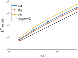
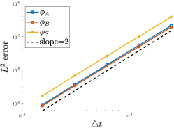
Refer to caption
(a) EQ
Refer to caption
(b) SVM1
Refer to caption
(c) SVM2
Refer to caption
(d) SVM3
Refer to caption
(e) SVM4
Figure 5.1: Temporal mesh refinement tests. The solution is computed up to t=1𝑡1t=1 with spatial mesh size h=1/2561256h=1/256 and variable time steps. Subplots show the mesh refinement test in time for the convergence rate of the EQ, SVM1, SVM2, SVM3, SVM4 scheme, respectively.
Refer to caption
(a) EQ
Refer to caption
(b) SVM1
Refer to caption
(c) SVM2
Refer to caption
(d) SVM3
Refer to caption
(e) SVM4
Figure 5.2: Spatial mesh refinement tests. The solution is computed up to t=1𝑡1t=1 at fixed time step t=104𝑡superscript104\triangle t=10^{-4}. Subplots show the mesh refinement test in space for the convergence rate of the EQ, SVM1, SVM2, SVM3, SVM4 scheme, respectively.

Taking T=1,t=104,h=1/128formulae-sequence𝑇1formulae-sequence𝑡superscript1041128T=1,~{}\triangle t=10^{-4},~{}h=1/128 and h=1/2561256h=1/256 respectively, we use Example 5.1 to examine the computational efficiency of the schemes. The results in CPU time(s) and convergence rate of supplementary variable α𝛼\alpha using each scheme are summarized in Figures 5.3 and 5.4, respectively. Firstly, α(t)𝛼𝑡\alpha(t) scales with C(h)Δt2𝐶Δsuperscript𝑡2C(h)\Delta t^{2} as expected. Secondly, C(h)𝐶C(h) decays with hh. Thirdly, SVM schemes compute faster than the EQ scheme on our workstation.
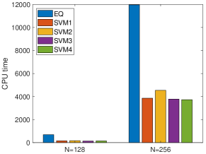
Refer to caption
Figure 5.3: For this model, SVM algorithms are more efficient than the EQ algorithm. In SVM algorithms, one solves a couple of linear system with all constant coefficients and a scalar nonlinear equation of the supplementary variable α𝛼\alpha. Whereas, in EQ algorithm, one solves a linear system with variable coefficients.
Refer to caption
(a) h=1/2561256h=1/256
Refer to caption
(b) N=128𝑁128N=128
Refer to caption
(c) N=256𝑁256N=256
Figure 5.4: Supplementary variable α𝛼\alpha obtained in SVM schemes are within the expected order (α𝒪(t2)similar-to𝛼𝒪superscript𝑡2\alpha\sim\mathcal{O}(\triangle t^{2})). In comparison, α𝛼\alpha in SVM1 and SVM2 algorithms is larger than that in SVM3 and SVM4 algorithms.

We use SVM2 algorithm with t=105,h=1/128formulae-sequence𝑡superscript1051128\triangle t=10^{-5},h=1/128 to conduct the following numerical investigations.

5.2 Dynamics of the copolymer solution

Notice that the volume fractions are dimensionless and we can easily nondimensionalize the model using the characteristic time and length scale. Thus, we assume the model we use in the numerical investigations are dimensionless as well. For details on the non-dimensionalization, please refer to [10]. We present 3 examples to show spot and lamellar structures in 2D copolymer solutions, which are present in copolymer melts as well. In this subsection, we fix the mobility matrix as

M=4×10³×diag[1,1,1].𝑀4superscript103diag111M=4\times 10^{-3}\times{\rm diag}[1,1,1]. (5.2)

All numerical experiments conducted by our algorithms respect energy dissipation rate and volume conservation although we do not show these in all examples.

Example 5.2 (Spots).
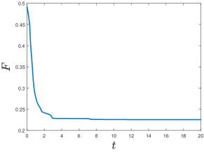
We set NA=2,NB=NS=1,χAA=χBB=χSS=0,χAB=6,χAS=4,χBS=8,ε=0.01,γ=103formulae-sequenceformulae-sequencesubscript𝑁𝐴2subscript𝑁𝐵subscript𝑁𝑆1subscript𝜒𝐴𝐴subscript𝜒𝐵𝐵subscript𝜒𝑆𝑆0formulae-sequencesubscript𝜒𝐴𝐵6formulae-sequencesubscript𝜒𝐴𝑆4formulae-sequencesubscript𝜒𝐵𝑆8formulae-sequence𝜀0.01𝛾superscript103N_{A}=2,~{}N_{B}=N_{S}=1,~{}\chi_{AA}=\chi_{BB}=\chi_{SS}=0,~{}\chi_{AB}=6,~{}\chi_{AS}=4,~{}\chi_{BS}=8,~{}\varepsilon=0.01,~{}\gamma=10^{3} and ϕA0=1/15+2/15(1cos2πx)(1cos2πy),ϕB0=0.5ϕA0,ϕS0=1ϕA0ϕB0formulae-sequencesubscriptsuperscriptitalic-ϕ0𝐴11521512𝜋𝑥12𝜋𝑦formulae-sequencesubscriptsuperscriptitalic-ϕ0𝐵0.5subscriptsuperscriptitalic-ϕ0𝐴subscriptsuperscriptitalic-ϕ0𝑆1subscriptsuperscriptitalic-ϕ0𝐴subscriptsuperscriptitalic-ϕ0𝐵\phi^{0}_{A}=1/15+2/15(1-\cos 2\pi x)(1-\cos 2\pi y),~{}\phi^{0}_{B}=0.5\phi^{0}_{A},~{}\phi^{0}_{S}=1-\phi^{0}_{A}-\phi^{0}_{B}. The free energy and volume conservation are shown in Figure 5.5. Some phase portraits are plotted in Figure 5.6.

Refer to caption
(a) free energy
Refer to caption
(b) average volume fractions
Figure 5.5: Energy decays and volume of each species conserves in t[0,20]𝑡020t\in[0,20], respectively.
Refer to caption
(a) ϕAϕBsubscriptitalic-ϕ𝐴subscriptitalic-ϕ𝐵\phi_{A}-\phi_{B}
Refer to caption
(b) ϕSsubscriptitalic-ϕ𝑆\phi_{S}
Figure 5.6: Microphase and macrophase separation at t=0.5,1,3,20𝑡0.51320t=0.5,~{}1,~{}3,~{}20. At the steady state, we observe spot structures in microphase separation that B𝐵B forms into spots surrounded by A𝐴A. In the 2nd row, the volume fraction of the solvent is shown.
Example 5.3 (Lamellae).

We set NA=NB=NS=1,χAA=χBB=χSS=0,χAB=χAS=6,χBS=8,ε=0.01,γ=104formulae-sequencesubscript𝑁𝐴subscript𝑁𝐵subscript𝑁𝑆1subscript𝜒𝐴𝐴subscript𝜒𝐵𝐵subscript𝜒𝑆𝑆0subscript𝜒𝐴𝐵subscript𝜒𝐴𝑆6formulae-sequencesubscript𝜒𝐵𝑆8formulae-sequence𝜀0.01𝛾superscript104N_{A}=N_{B}=N_{S}=1,~{}\chi_{AA}=\chi_{BB}=\chi_{SS}=0,~{}\chi_{AB}=\chi_{AS}=6,~{}\chi_{BS}=8,~{}\varepsilon=0.01,~{}\gamma=10^{4} and ϕA0=ϕB0=3/16+1/16(1cos2πx)(1cos2πy),ϕS0=1ϕA0ϕB0formulae-sequencesubscriptsuperscriptitalic-ϕ0𝐴subscriptsuperscriptitalic-ϕ0𝐵31611612𝜋𝑥12𝜋𝑦subscriptsuperscriptitalic-ϕ0𝑆1subscriptsuperscriptitalic-ϕ0𝐴subscriptsuperscriptitalic-ϕ0𝐵\phi^{0}_{A}=\phi^{0}_{B}=3/16+1/16(1-\cos 2\pi x)(1-\cos 2\pi y),~{}\phi^{0}_{S}=1-\phi^{0}_{A}-\phi^{0}_{B}. Some phase portraits are plotted in Figure 5.7.

Refer to caption
(a) ϕAϕBsubscriptitalic-ϕ𝐴subscriptitalic-ϕ𝐵\phi_{A}-\phi_{B}
Refer to caption
(b) ϕSsubscriptitalic-ϕ𝑆\phi_{S}
Figure 5.7: Microphase and macrophase separation at t=1,20,40,80𝑡1204080t=1,~{}20,~{}40,~{}80. At the steady state, we observe lamellar structures in microphase separation that both A𝐴A and B𝐵B forms into lamellae. The solvent volume fraction is shown in the 2nd row.
Example 5.4 (Lamellae+spots).

We set NA=NB=NS=1,χAA=χBB=χSS=0,χAB=χAS=6,χBS=8,ε=0.01,γ=103formulae-sequencesubscript𝑁𝐴subscript𝑁𝐵subscript𝑁𝑆1subscript𝜒𝐴𝐴subscript𝜒𝐵𝐵subscript𝜒𝑆𝑆0subscript𝜒𝐴𝐵subscript𝜒𝐴𝑆6formulae-sequencesubscript𝜒𝐵𝑆8formulae-sequence𝜀0.01𝛾superscript103N_{A}=N_{B}=N_{S}=1,~{}\chi_{AA}=\chi_{BB}=\chi_{SS}=0,~{}\chi_{AB}=\chi_{AS}=6,~{}\chi_{BS}=8,~{}\varepsilon=0.01,~{}\gamma=10^{3} and ϕA0=ϕB0=0.05+0.1(1cos2πx)(1cos2πy),ϕS0=1ϕA0ϕB0formulae-sequencesubscriptsuperscriptitalic-ϕ0𝐴subscriptsuperscriptitalic-ϕ0𝐵0.050.112𝜋𝑥12𝜋𝑦subscriptsuperscriptitalic-ϕ0𝑆1subscriptsuperscriptitalic-ϕ0𝐴subscriptsuperscriptitalic-ϕ0𝐵\phi^{0}_{A}=\phi^{0}_{B}=0.05+0.1(1-\cos 2\pi x)(1-\cos 2\pi y),~{}\phi^{0}_{S}=1-\phi^{0}_{A}-\phi^{0}_{B}. Some phase portraits are plotted in Figure 5.8.

Refer to caption
(a) ϕAϕBsubscriptitalic-ϕ𝐴subscriptitalic-ϕ𝐵\phi_{A}-\phi_{B}
Refer to caption
(b) ϕSsubscriptitalic-ϕ𝑆\phi_{S}
Figure 5.8: Microphase and macrophase separation at t=1,2,5,20𝑡12520t=1,~{}2,~{}5,~{}20. At the steady state, we observe both lamellar and spot structures in microphase separation that there is an A𝐴A spot in the core surrounded by B𝐵B lamellae and there are 4 B𝐵B spots separated by A𝐴A lamellae scattered on the edge of the circular copolymer area.

5.3 Cross-coupling effect in mobility on dynamics

In the past, nearly all numerical simulations on dynamics of copolymers focused on a mobility matrix without the cross-coupling effect, i.e., the mobility coefficient matrix is a diagonal matrix. Likewise, the corresponding friction matrix is diagonal as well. Given the fact that there exists friction between different species of polymers and long range interaction in the copolymer solution, we would like to know how the chemical potential derived from one species affects the dynamics of the other so as to impact on the overall dynamics in the mixture. This in fact investigates how forces generated from chemical potentials of different species impact on dynamics of the other species via frictions.

Notice that M𝑀M is the inverse of the friction matrix. So qualitatively, the smaller the molecule is, the larger the corresponding Miisubscript𝑀𝑖𝑖M_{ii} should be. In theory, mobility matrices dictate dynamical paths of the system while relaxing back to the steady state. We all know that the steady state is determined by the free energy while the path towards the steady state in the phase space is dictated by the mobility. In this subsection, we choose mobility matrices with diagonally dominant elements and the cross-coupling effect is represented by the off-diagonal entries.

Example 5.5 (Cross-coupling effect in mobility).

We set NA=3,NB=2,NS=1,χAA=χBB=χSS=0,χAB=4,χAS=6,χBS=8,ε=0.01,γ=104formulae-sequenceformulae-sequencesubscript𝑁𝐴3formulae-sequencesubscript𝑁𝐵2formulae-sequencesubscript𝑁𝑆1subscript𝜒𝐴𝐴subscript𝜒𝐵𝐵subscript𝜒𝑆𝑆0formulae-sequencesubscript𝜒𝐴𝐵4formulae-sequencesubscript𝜒𝐴𝑆6formulae-sequencesubscript𝜒𝐵𝑆8formulae-sequence𝜀0.01𝛾superscript104N_{A}=3,~{}N_{B}=2,~{}N_{S}=1,~{}\chi_{AA}=\chi_{BB}=\chi_{SS}=0,~{}\chi_{AB}=4,~{}\chi_{AS}=6,~{}\chi_{BS}=8,~{}\varepsilon=0.01,~{}\gamma=10^{4} and ϕA0=3/14+3/35(1cos2πx)(1cos2πy),ϕB0=2/3ϕA0,ϕS0=1ϕA0ϕB0formulae-sequencesubscriptsuperscriptitalic-ϕ0𝐴31433512𝜋𝑥12𝜋𝑦formulae-sequencesubscriptsuperscriptitalic-ϕ0𝐵23subscriptsuperscriptitalic-ϕ0𝐴subscriptsuperscriptitalic-ϕ0𝑆1subscriptsuperscriptitalic-ϕ0𝐴subscriptsuperscriptitalic-ϕ0𝐵\phi^{0}_{A}=3/14+3/35(1-\cos 2\pi x)(1-\cos 2\pi y),~{}\phi^{0}_{B}=2/3\phi^{0}_{A},~{}\phi^{0}_{S}=1-\phi^{0}_{A}-\phi^{0}_{B}. We take 6 different mobility matrices respectively given by

M1:103×[444],M2:103×[345],M3:103×[30.50.545],M4:103×[30.50.50.540.50.50.55],M5:103×[30.50.545],M6:103×[30.50.50.540.50.50.55].:𝑀1superscript103delimited-[]matrix4missing-subexpressionmissing-subexpressionmissing-subexpression4missing-subexpressionmissing-subexpressionmissing-subexpression4𝑀2:superscript103delimited-[]matrix3missing-subexpressionmissing-subexpressionmissing-subexpression4missing-subexpressionmissing-subexpressionmissing-subexpression5𝑀3:superscript103delimited-[]matrix30.5missing-subexpression0.54missing-subexpressionmissing-subexpressionmissing-subexpression5𝑀4:superscript103delimited-[]matrix30.50.50.540.50.50.55𝑀5:superscript103delimited-[]matrix30.5missing-subexpression0.54missing-subexpressionmissing-subexpressionmissing-subexpression5𝑀6:superscript103delimited-[]matrix30.50.50.540.50.50.55\begin{gathered}M1:10^{-3}\!\times\!\left[\begin{matrix}4&&\\ &4&\\ &&4\end{matrix}\right],~{}M2:10^{-3}\!\times\!\left[\begin{matrix}3&&\\ &4&\\ &&5\end{matrix}\right],~{}M3:10^{-3}\!\times\!\left[\begin{matrix}3&-0.5&\\ -0.5&4&\\ &&5\end{matrix}\right],\\ M4:10^{-3}\!\times\!\left[\begin{matrix}3&-0.5&-0.5\\ -0.5&4&-0.5\\ -0.5&-0.5&5\end{matrix}\right],~{}M5:10^{-3}\!\times\!\left[\begin{matrix}3&0.5&\\ 0.5&4&\\ &&5\end{matrix}\right],~{}M6:10^{-3}\!\times\!\left[\begin{matrix}3&0.5&0.5\\ 0.5&4&0.5\\ 0.5&0.5&5\end{matrix}\right].\end{gathered} (5.3)

Some phase portraits and free energies are plotted in Figures 5.9, 5.10 and 5.11, respectively.

Refer to caption
(a) M1𝑀1M1
Refer to caption
(b) M2𝑀2M2
Refer to caption
(c) M3𝑀3M3
Refer to caption
(d) M4𝑀4M4
Refer to caption
(e) M5𝑀5M5
Refer to caption
(f) M6𝑀6M6
Figure 5.9: ϕAϕBsubscriptitalic-ϕ𝐴subscriptitalic-ϕ𝐵\phi_{A}-\phi_{B} at t=4,25,45,120𝑡42545120t=4,~{}25,~{}45,~{}120 with respect to 6 different mobilites. From the core parts of the copolymer area, we observe different microscopic phase separations in transient dynamics decided by 6 different mobilities (It is helpful to observe macrophase separations simultaneously). At t=120𝑡120t=120, all 6 steady state structures are similar with (a)(b)(f) are 90 degree rotation of (c)(d)(e). Since there is no external field is present, the steady states are essentially the same modulo a rotational motion.
Refer to caption
(a) M1𝑀1M1
Refer to caption
(b) M2𝑀2M2
Refer to caption
(c) M3𝑀3M3
Refer to caption
(d) M4𝑀4M4
Refer to caption
(e) M5𝑀5M5
Refer to caption
(f) M6𝑀6M6
Figure 5.10: ϕSsubscriptitalic-ϕ𝑆\phi_{S} at t=4,25,45,120𝑡42545120t=4,~{}25,~{}45,~{}120 with respect to 6 different mobilites. Macroscopic phase separations are different in transient dynamics deictated by 6 different mobilities. At t=120𝑡120t=120, they are all the same.
Refer to caption
Figure 5.11: Free energies in t[0,120]𝑡0120t\in[0,120]. There are slight differences among the results quantitatively.

Figure 5.9 shows the microscopic phase separation between A𝐴A and B𝐵B polymers, while Figure 5.10 shows the macroscopic phase separation between the copolymer and the solvent. At t=120𝑡120t=120, the system reaches the metastable/steady state, which is determined by the free energy. In this example, all mobilities eventually lead to the same metastable/steady state as expected since mobility is instrumental to transient dynamics not to the final steady state. During transient dynamics, the free energy decays with time as shown in Figure 5.11.

We reiterate that different mobilities result in different dynamics, while different mobilities do not necessarily lead to different metastable/steady state. In fact, if the steady state is globally stable and unique, it is independent of the mobility. In Example 5.6 and Example 5.7, 3 different mobilities also lead to the same steady state. However, different mobilities lead to different metastable states as depicted in Figure 5.9(b)(c), dictated by mobilities M2,M3𝑀2𝑀3M2,M3. For discussion about metastable states and energy landscapes, we suggest readers refer to [34, 7, 46, 47].

5.4 Dynamics of the copolymer solution coupled with the electric field

When an electric field is applied to the copolymer solution, patterns normally emerge in long time. During the transient state from an irregular phase morphology to lamellar patterns, branches are formed momentarily and annihilated eventually by the electric field. This is a process of defect removal in material processing, where one refers to the branches as defects. In the following example, we would like to showcase the process at selected time slots.

Example 5.6 (Pattern formation driven by the electric field).

We set NA=15,NB=10,NS=1,χAA=χBB=χSS=0,χAB=1,χAS=2,χBS=4,ε=0.01,γ=105,ϵ0=ϵ1=1,𝐄0=[10,20]formulae-sequenceformulae-sequencesubscript𝑁𝐴15formulae-sequencesubscript𝑁𝐵10formulae-sequencesubscript𝑁𝑆1subscript𝜒𝐴𝐴subscript𝜒𝐵𝐵subscript𝜒𝑆𝑆0formulae-sequencesubscript𝜒𝐴𝐵1formulae-sequencesubscript𝜒𝐴𝑆2formulae-sequencesubscript𝜒𝐵𝑆4formulae-sequence𝜀0.01formulae-sequence𝛾superscript105subscriptitalic-ϵ0subscriptitalic-ϵ11subscript𝐄0superscript1020topN_{A}=15,~{}N_{B}=10,~{}N_{S}=1,~{}\chi_{AA}=\chi_{BB}=\chi_{SS}=0,~{}\chi_{AB}=1,~{}\chi_{AS}=2,~{}\chi_{BS}=4,~{}\varepsilon=0.01,~{}\gamma=10^{5},~{}\epsilon_{0}=\epsilon_{1}=1,~{}\bm{E}_{0}=[10,20]^{\top} and

mobility1:104×[4620],mobility2:104×[411620],mobility3:104×[4111611120].:mobility1superscript104delimited-[]matrix4missing-subexpressionmissing-subexpressionmissing-subexpression6missing-subexpressionmissing-subexpressionmissing-subexpression20mobility2:superscript104delimited-[]matrix41missing-subexpression16missing-subexpressionmissing-subexpressionmissing-subexpression20mobility3:superscript104delimited-[]matrix4111611120{\rm mobility}~{}1\!:\!10^{-4}\!\times\!\left[\begin{matrix}4&&\\ &6&\\ &&20\end{matrix}\right]\!,~{}{\rm mobility}~{}2\!:\!10^{-4}\!\times\!\left[\begin{matrix}4&-1&\\ -1&6&\\ &&20\end{matrix}\right]\!,~{}{\rm mobility}~{}3\!:\!10^{-4}\!\times\!\left[\begin{matrix}4&-1&-1\\ -1&6&-1\\ -1&-1&20\end{matrix}\right]\!. (5.4)

The initial conditions are

ϕA0=0.3+0.001×rand(x,y),ϕB0=0.2+0.001×rand(x,y),ϕS0=1ϕA0ϕB0,formulae-sequencesubscriptsuperscriptitalic-ϕ0𝐴0.30.001rand𝑥𝑦formulae-sequencesubscriptsuperscriptitalic-ϕ0𝐵0.20.001rand𝑥𝑦subscriptsuperscriptitalic-ϕ0𝑆1subscriptsuperscriptitalic-ϕ0𝐴subscriptsuperscriptitalic-ϕ0𝐵\displaystyle\phi^{0}_{A}=0.3+0.001\times{\rm rand}(x,y),\quad\phi^{0}_{B}=0.2+0.001\times{\rm rand}(x,y),\quad\phi^{0}_{S}=1-\phi^{0}_{A}-\phi^{0}_{B}, (5.5)

where rand(x,y)(1,1)rand𝑥𝑦11{\rm rand}(x,y)\in(-1,1) denotes a random number generator that follows the uniform distribution. Some phase portraits and the total energy are plotted in Figures 5.12, 5.13 and 5.14. Notice that the imposed electric field is slanted in this example.

Refer to caption
(a) mobility 1
Refer to caption
(b) mobility 2
Refer to caption
(c) mobility 3
Figure 5.12: ϕAϕBsubscriptitalic-ϕ𝐴subscriptitalic-ϕ𝐵\phi_{A}-\phi_{B} at t=12,15,22,200𝑡121522200t=12,~{}15,~{}22,~{}200 in dynamics with respect to 3 different mobilities. Defects in the microscopic phase separation are observed in transient. The electric field irons out the defect branches. The system generates a lamellar pattern in the steady state.
Refer to caption
(a) mobility 1
Refer to caption
(b) mobility 2
Refer to caption
(c) mobility 3
Figure 5.13: ϕSsubscriptitalic-ϕ𝑆\phi_{S} at t=12,15,22,200𝑡121522200t=12,~{}15,~{}22,~{}200 in dynamics with respect to 3 different mobilities. Defects in the macroscopic phase separation are observed in transient. Final lamellar patterned phase portraits are obtained through the Ostwald ripening.
Refer to caption
Figure 5.14: Energies in t[0,200]𝑡0200t\in[0,200] with respect to 3 different mobilities.

Under the electric field, lamellar stripes emerge and so do defects. Defects move along the direction of the electric field and disappear at the boundary of the computational domain. The number of defects decreases to 00 eventually and the morphology of the final meso-structures maintain a lamellar pattern with stripes along the direction of the electric field. The free energy curves decay with time as shown in Figure 5.14.

5.5 Dynamics of the copolymer solution coupled with the magnetic field

Like the electric field, the magnetic field aligns the copolymer in the solution and eliminate transient defects as well.

Example 5.7 (Pattern formation driven by the magnetic field).

We set NA=15,NB=10,NS=1,χAA=χBB=χSS=0,χAB=1,χAS=2,χBS=4,ε=0.01,γ=105formulae-sequenceformulae-sequencesubscript𝑁𝐴15formulae-sequencesubscript𝑁𝐵10formulae-sequencesubscript𝑁𝑆1subscript𝜒𝐴𝐴subscript𝜒𝐵𝐵subscript𝜒𝑆𝑆0formulae-sequencesubscript𝜒𝐴𝐵1formulae-sequencesubscript𝜒𝐴𝑆2formulae-sequencesubscript𝜒𝐵𝑆4formulae-sequence𝜀0.01𝛾superscript105N_{A}=15,~{}N_{B}=10,~{}N_{S}=1,~{}\chi_{AA}=\chi_{BB}=\chi_{SS}=0,~{}\chi_{AB}=1,~{}\chi_{AS}=2,~{}\chi_{BS}=4,~{}\varepsilon=0.01,~{}\gamma=10^{5} and γm=103,𝐁0=[1,0]formulae-sequencesubscript𝛾𝑚superscript103subscript𝐁0superscript10top\gamma_{m}=10^{-3},~{}\bm{B}_{0}=[1,0]^{\top}. We use mobility matrices in (5.4) and initial conditions in (5.5). Some phase portraits and the total energy are plotted in Figures 5.15, 5.16 and 5.17. Notice the magnetic field is aligned in the x𝑥x-direction in this simulation.

Refer to caption
(a) mobility 1
Refer to caption
(b) mobility 2
Refer to caption
(c) mobility 3
Figure 5.15: ϕAϕBsubscriptitalic-ϕ𝐴subscriptitalic-ϕ𝐵\phi_{A}-\phi_{B} at t=2.5,3.5,10,100𝑡2.53.510100t=2.5,~{}3.5,~{}10,~{}100. Microscopic phase separation is shown for 3 different mobilities.
Refer to caption
(a) mobility 1
Refer to caption
(b) mobility 2
Refer to caption
(c) mobility 3
Figure 5.16: ϕSsubscriptitalic-ϕ𝑆\phi_{S} at t=2.5,3.5,10,100𝑡2.53.510100t=2.5,~{}3.5,~{}10,~{}100. Macroscopic phase separation is shown for 3 different mobilities.
Refer to caption
Figure 5.17: Energies in t[0,100]𝑡0100t\in[0,100] with respect to 3 different mobilities.

The effect of the magnetic field is similar to that of the electric field in that it induces lamellar stripes in the final state. During transient dynamics, both lamellar structures and defects emerge. Defects move along the direction of the magnetic field and disappear at the boundary of the computational domain. The number of defects eventually decreases to 00 and the morphology of the lamellar structure shows stripes in the direction of the imposed magnetic field. The energy curves decay to a steady state as shown in Figure 5.17.

5.6 Hysteresis effect related to the electric field

In this example, we use the electric field coupled model to simulate the hysteresis effect due to the increase and decrease of the strength of an electric field. First, taking the steady state denoted as S1subscript𝑆1S_{1} in Example 5.2 as the initial condition, we add an electric field 𝑬0(t)subscript𝑬0𝑡\bm{E}_{0}(t) to drive state S1subscript𝑆1S_{1} into a new state S2subscript𝑆2S_{2}. Then, we shut down the electric field and we expect structure S2subscript𝑆2S_{2} relaxes back to S1subscript𝑆1S_{1}.

Example 5.8 (Hysteresis effect).

We set NA=2,NB=NS=1,χAA=χBB=χSS=0,χAB=6,χAS=4,χBS=8,ε=0.01,γ=103,ϵ0=1,ϵ1=0.6formulae-sequenceformulae-sequencesubscript𝑁𝐴2subscript𝑁𝐵subscript𝑁𝑆1subscript𝜒𝐴𝐴subscript𝜒𝐵𝐵subscript𝜒𝑆𝑆0formulae-sequencesubscript𝜒𝐴𝐵6formulae-sequencesubscript𝜒𝐴𝑆4formulae-sequencesubscript𝜒𝐵𝑆8formulae-sequence𝜀0.01formulae-sequence𝛾superscript103formulae-sequencesubscriptitalic-ϵ01subscriptitalic-ϵ10.6N_{A}=2,~{}N_{B}=N_{S}=1,~{}\chi_{AA}=\chi_{BB}=\chi_{SS}=0,~{}\chi_{AB}=6,~{}\chi_{AS}=4,~{}\chi_{BS}=8,~{}\varepsilon=0.01,~{}\gamma=10^{3},~{}\epsilon_{0}=1,~{}\epsilon_{1}=0.6. We use the mobility matrix in (5.2) and take the numerical solution at t=20𝑡20t=20 from Example 5.2 as the initial condition of this example. The imposed electric field is given by 𝐄0(t)=[E1(t),0]subscript𝐄0𝑡superscriptsubscript𝐸1𝑡0top\bm{E}_{0}(t)=[E_{1}(t),0]^{\top} where

E1(t)={2t,0t5,10,5t15,402t,15t20,0,t20.E_{1}(t)=\left\{\begin{aligned} &2t,&&0\leq t\leq 5,\\ &10,&&5\leq t\leq 15,\\ &40-2t,&&15\leq t\leq 20,\\ &0,&&t\geq 20.\end{aligned}\right. (5.6)

Some phase portraits at different time frames and the total energy are plotted in Figures 5.18, 5.19 and 5.20. The magnitudes of the electric field and induced electric field are presented in Figure 5.21.

Refer to caption
(a) ϕAϕBsubscriptitalic-ϕ𝐴subscriptitalic-ϕ𝐵\phi_{A}-\phi_{B}
Refer to caption
(b) ϕSsubscriptitalic-ϕ𝑆\phi_{S}
Figure 5.18: Microphase and macrophase separation at t=1.3,5,15,20𝑡1.351520t=1.3,~{}5,~{}15,~{}20 after the electric field is imposed. The electric field stretches the given spot structures into lamellar stripes.
Refer to caption
(a) ϕAϕBsubscriptitalic-ϕ𝐴subscriptitalic-ϕ𝐵\phi_{A}-\phi_{B}
Refer to caption
(b) ϕSsubscriptitalic-ϕ𝑆\phi_{S}
Figure 5.19: Microphase and macrophase separation at t=22,25,35,70𝑡22253570t=22,~{}25,~{}35,~{}70 after the imposed electric field is reversed. Without the electric field, the lamellar stripe structures gradually relax back to spot structures. However, the time it takes for S2subscript𝑆2S_{2} to relax back to S1subscript𝑆1S_{1} is much longer than it evolves from S1subscript𝑆1S_{1} to S2subscript𝑆2S_{2}.
Refer to caption
(a) 20t7020𝑡70-20\leq t\leq 70
Refer to caption
(b) 20t020𝑡0-20\leq t\leq 0
Refer to caption
(c) 5t155𝑡155\leq t\leq 15
Refer to caption
(d) 20t7020𝑡7020\leq t\leq 70
Figure 5.20: Energy in t[20,70]𝑡2070t\in[-20,70]. We use “t[20,0]𝑡200t\in[-20,0]” to substitute expression “t[0,20]𝑡020t\in[0,20]” from Example 5.2 to display the energy evolution. The result shows that the energy is not symmetric with respect to t[0,20]𝑡020t\in[0,20].
Refer to caption
(a) 𝑬0Φnormsubscript𝑬0Φ\|\bm{E}_{0}-\nabla\Phi\|
Refer to caption
(b) ΦnormΦ\|\nabla\Phi\|
Figure 5.21: Magnitudes (discrete L2superscript𝐿2L^{2} norm) of the electric field 𝑬=𝑬0Φ𝑬subscript𝑬0Φ\bm{E}=\bm{E}_{0}-\nabla\Phi and induced electric field ΦΦ\nabla\Phi in t[0,20]𝑡020t\in[0,20]. The magnitude of induced electric field ΦnormΦ\|\nabla\Phi\| is small compared to 𝑬0Φnormsubscript𝑬0Φ\|\bm{E}_{0}-\nabla\Phi\|, but not negligible.

Notice that the induced electric potential ΦΦ\Phi satisfies (2.26), i.e.

[(ϵ0+ϵ1(ϕAϕBϕ¯A+ϕ¯B))(𝑬0Φ)]=0.delimited-[]subscriptitalic-ϵ0subscriptitalic-ϵ1subscriptitalic-ϕ𝐴subscriptitalic-ϕ𝐵subscript¯italic-ϕ𝐴subscript¯italic-ϕ𝐵subscript𝑬0Φ0\nabla\cdot\Big{[}\big{(}\epsilon_{0}+\epsilon_{1}(\phi_{A}-\phi_{B}-\overline{\phi}_{A}+\overline{\phi}_{B})\big{)}(\bm{E}_{0}-\nabla\Phi)\Big{]}=0. (5.7)

So ΦΦ\Phi implies some mesoscopic structure properties of the system. We observe that curve 𝑬0Φnormsubscript𝑬0Φ\|\bm{E}_{0}-\nabla\Phi\| in Figure 5.21(a) appears to be symmetric about t=10𝑡10t=10 at large scale, while curve ΦnormΦ\|\nabla\Phi\| in Figure 5.21(b) does not in fine scale. The asymmetry in the relaxation dynamics of the morphology of transient states and the induced electric field confirm the existence of hysteresis effect with respect to the increase and decrease of the electric field.

6 Conclusion

We have derived thermodynamically consistent models for diblock copolymer solutions coupled with the electric and magnetic field, respectively, using the generalized Onsager principle. We then devised a series of structure-preserving numerical algorithms for the models to preserve their energy dissipation rates using the EQ method and the supplementary variable method (SVM), respectively. Like EQ, SVM provides a paradigm for one to develop structure-preserving numerical algorithms that preserve the thermodynamical consistency of the models after discretization. Numerical experiments using the SVM scheme are performed to confirm the convergence rates and reveal the impact of the mobility, the electric and magnetic fields on controlling dynamics of the copolymer solution.

Acknowledgements

This research is partially supported by the National Natural Science Foundation of China (award 11971051 and NSAF-U1930402). Qi Wang’s research is partially supported by a DOE grant (DE-SC0020272), National Science Foundation grants (award DMS-1815921 and OIA-1655740) and a GEAR award from SC EPSCoR/IDeA Program.

References

  • [1] Santiago Badia, Francisco Guillén-González, and Juan Vicente Gutiérrez-Santacreu. Finite element approximation of nematic liquid crystal flows using a saddle-point structure. J. Comput. Phys., 230(41):1686–1706, 2011.
  • [2] A. Böker, H. Elbs, H. Hänsel, A. Knoll, S. Ludwigs, H. Zettl, A. V. Zvelindovsky, G. J. A. Sevink, V. Urban, V. Abetz, A. H. E. Müller, and G. Krausch. Electric field induced alignment of concentrated block copolymer solutions. Macromolecules, 36(21):8078–8087, 2003.
  • [3] Chuanjun Chen, Xi Li, Jun Zhang, and Xiaofeng Yang. Efficient linear, decoupled, and unconditionally stable scheme for a ternary Cahn-Hilliard type Nakazawa-Ohta phase-field model for tri-block copolymers. Appl. Math. Comput., 388(1):125463, 2021.
  • [4] Chuanjun Chen, Jun Zhang, and Xiaofeng Yang. Efficient numerical scheme for a new hydrodynamically-coupled conserved Allen–Cahn type Ohta–Kawaski phase-field model for diblock copolymer melt. Comput. Phys. Commun., 256:107418, 2020.
  • [5] Qing Cheng, Chun Liu, and Jie Shen. A new Lagrange multiplier approach for gradient flows. Comput. Methods Appl. Mech. Engrg., 367:113070, 2020.
  • [6] Qing Cheng, Xiaofeng Yang, and Jie Shen. Efficient and accurate numerical schemes for a hydro-dynamically coupled phase field diblock copolymer model. J. Comput. Phys., 341:44–60, 2017.
  • [7] Rustum Choksi, Mirjana Maras, and J. F. Williams. 2D phase diagram for minimizers of a Cahn–Hilliard functional with long-range interactions. Siam J. Appl. Dyn. Syst., 10(4):1344–1362, 2011.
  • [8] Rustum Choksi, Mark A. Peletier, and J. F. Williams. On the phase diagram for microphase separation of diblock copolymers: an approach via a nonlocal Cahn–Hilliard functional. Siam J. Appl. Math., 69(6):1712–1738, 2009.
  • [9] Rustum Choksi and Xiaofeng Ren. On the derivation of a density functional theory for microphase separation of diblock copolymers. J. Stat. Phys., 113(1-2):151–176, 2003.
  • [10] Rustum Choksi and Xiaofeng Ren. Diblock copolymer/homopolymer blends: derivation of a density functional theory. Physica D, 203(1-2):100–119, 2005.
  • [11] Maria Inês Martins Copetti and Charlie M. Elliott. Numerical analysis of the Cahn-Hilliard equation with a logarithmic free energy. Numer. Math., 63(1):39–65, 1992.
  • [12] Niloufar Faghihi, Simiso Mkhonta, Ken R. Elder, and Martin Grant. Magnetic islands modelled by a phase-field-crystal approach. Eur. Phys. J. B, 91:55, 2018.
  • [13] Yuezheng Gong, Qi Hong, and Qi Wang. Supplementary variable method for developing structure-preserving numerical approximations to thermodynamically consistent partial differential equations. arXiv:2006.04348, 2020.
  • [14] Francisco Guillén-González and Giordano Tierra. On linear schemes for a Cahn-Hilliard diffuse interface model. J. Comput. Phys., 234:140–171, 2013.
  • [15] Francisco Guillén-González and Giordano Tierra. Second order schemes and time-step adaptivity for Allen–Cahn and Cahn–Hilliard models. Comput. Math. Appl., 68(8):821–846, 2013.
  • [16] Ernst Hairer, Christian Lubich, and Gerhard Wanner. Geometric numerical integration: structure-preserving algorithms for ordinary differential equations. Springer, 2006.
  • [17] Ian W. Hamley. The physics of block copolymers. Oxfor University Press, 1998.
  • [18] Ian W. Hamley. Developments in block copolymer science and technology. John Wiley, 2004.
  • [19] Ian W. Hamley. Block copolymers in solution: fundamentals and applications. John Wiley, 2005.
  • [20] Qi Hong, Jun Li, and Qi Wang. Supplementary variable method for structure-preserving approximations to partial differential equations with deduced equations. Appl. Math. Lett., 110:106576, 2020.
  • [21] Lev Davidovich Landau and Evgenii Mikhaílovich Lifshitz. Electrodynamics of continuous media. Elsevier, 1984.
  • [22] Dung Q. Ly and Charalampos Makatsoris. Effects of the homopolymer molecular weight on a diblock copolymer in a 3D spherical confinement. BMC Chem., 13(1):24, 2019.
  • [23] Takao Ohta and Kyozi Kawasaki. Equilibrium morphology of block copolymer melts. Macromolecules, 19(10):2621–2632, 1986.
  • [24] Takao Ohta and Makiko Nonomura. Elastic property of bilayer membrane in copolymer-homopolymer mixtures. Eur. Phys. J. B, 2(1):57–68, 1998.
  • [25] Lars Onsager. Reciprocal relations in irreversible processes. I. Phys. Rev., 37:405–426, 1931.
  • [26] Lars Onsager. Reciprocal relations in irreversible processes. II. Phys. Rev., 38:2265–2279, 1931.
  • [27] Lars Onsager and Stefan Machlup. Fluctuations and irreversible processes. Phys. Rev., 91:1505–1512, 1953.
  • [28] Saulo Orizaga and Karl Glasner. Instability and reorientation of block copolymer microstructure by imposed electric fields. Phys. Rev. E, 93(5):052504, 2016.
  • [29] Christian W. Pestera, Clemens Liedel, Markus Ruppel, and Alexander Böker. Block copolymers in electric fields. Prog. Polym. Sci., 64:182–214, 2017.
  • [30] Marco Pinna, Ludwig Schreier, and Andrei V. Zvelindovsky. Mechanisms of electric-field-induced alignment of block copolymer lamellae. Soft Matter, 5:970–973, 2009.
  • [31] Matthew Seymour, F. Sanches, Ken Elde, and Nikolas Provatas. Phase-field crystal approach for modeling the role of microstructure in multiferroic composite materials. Phys. Rev. E, 92:184109, 2015.
  • [32] Jie Shen, Jie Xu, and Jiang Yang. The scalar auxiliary variable (SAV) approach for gradient flows. J. Comput. Phys., 353:407–416, 2018.
  • [33] Jie Shen, Jie Xu, and Jiang Yang. A new class of efficient and robust energy stable schemes for gradient flows. Siam Rev., 61(3):474–506, 2019.
  • [34] David Shirokoff, Rustum Choksi, and Jean-Christophe Nave. Sufficient conditions for global minimality of metastable states in a class of non-convex functionals: a simple approach via quadratic lower bounds. J. Nonlinear Sci., 25(3):539–582, 2015.
  • [35] Jan Bouwe van den Berg and J. F. Williams. Validation of the bifurcation diagram in the 2D Ohta–Kawasaki problem. Nonlinearty, 30(4):1584–1638, 2017.
  • [36] Jan Bouwe van den Berg and J. F. Williams. Rigorously computing symmetric stationary states of the Ohta-Kawasaki problem in three dimensions. Siam J. Math. Aanl., 51(1):131–158, 2019.
  • [37] Qi Wang. Generalized onsager principle and its applications. In Xiangyang Liu, editor, Frontiers and progress of current soft matter research, chapter 3. Springer Singapore, 2021.
  • [38] Jiaping Wu, Zheng Wang, Yuhua Yin, Run Jiang, Baohui Li, and An chang Shi. A simulation study of phase behavior of double-hydrophilic block copolymers in aqueous solutions. Macromolecules, 48(24):8897–8906, 2014.
  • [39] Xiangfa Wu and Yuris A. Dzenis. Phase-field modeling of the formation of lamellar nanostructures in diblock copolymer thin films under inplanar electric fields. Phys. Rev. E, 77(511):031807, 2008.
  • [40] Ting Xu, A. V. Zvelindovsky, G. J. A. Sevink, Oleg Gang, Ben Ocko, Yuqing Zhu, Samuel P. Gido, and Thomas P. Russell. Electric field induced sphere-to-cylinder transition in diblock copolymer thin films. Macromolecules, 37(18):6980–6984, 2004.
  • [41] Ting Xu, A. V. Zvelindovsky, G. J. A. Sevink, K. S. Lyakhova, H. Jinnai, and Thomas P. Russell. Electric field alignment of asymmetric diblock copolymer thin films. Macromolecules, 38(26):10788–10798, 2005.
  • [42] Kohtaro Yamada, Emiko Yasuno Youhei Kawabata, and Tohru Okuzono Tadashi Kato. Mesoscopic simulation of phase behaviors and structures in an amphiphile-solvent system. Phys. Rev. E, 89(6):062310, 2014.
  • [43] Xiaofeng Yang and Jia Zhao. On linear and unconditionally energy stable algorithms for variable mobility Cahn-Hilliard equation with logarithmic Flory-Huggins potential. Comm. Comp. Phys., 25:703–728, 2019.
  • [44] Xiaogang Yang, Jun Li, M. Gregory Forest, and Qi Wang. Hydrodynamic theories for flows of active liquid crystals and the Generalized Onsager principle. Entropy, 18(6):202, 2016.
  • [45] Zhiguo Yang and Suchuan Dong. A roadmap for discretely energy-stable schemes for dissipative systems based on a generalized auxiliary variable with guaranteed positivity. J. Comput. Phys., 404:109121, 2020.
  • [46] Jianyuan Yin, Yiwei Wang, Jeff Z. Y. Chen, Pingwen Zhang, and Lei Zhang. Construction of a pathway map on a complicated energy landscape. Phys. Rev. Lett., 124(9):090601, 2020.
  • [47] Bing Yu and Lei Zhang. Global optimization-based dimer method for finding saddle points. Discrete Cont. Dyn.-B, 26(1):741–753, 2021.
  • [48] Jun Zhang, Chuanjun Chen, and Xiaofeng Yang. Efficient and energy stable method for the Cahn-Hilliard phase-field model for diblock copolymers. Appl. Numer. Math., 151:263–281, 2020.
  • [49] Jun Zhang, Chuanjun Chen, Xiaofeng Yang, and Kejia Pan. Efficient numerical scheme for a penalized Allen–Cahn type Ohta–Kawasaki phase-field model for diblock copolymers. J. Comput. Appl. Math., 378:112905, 2020.
  • [50] Jun Zhang and Xiaofeng Yang. A new magnetic-coupled Cahn–Hilliard phase-field model for diblock copolymers and its numerical approximations. Appl. Math. Lett., 107:106412, 2020.
  • [51] Jia Zhao, Xiaofeng Yang, Yuezheg Gong, Xueping Zhao, Xiaogang Yang, Jun Li, and Qi Wang. A general strategy for numerical approximations of non-equilibrium models–part i: thermodynamical systems. Int. J. Numer. Anal. Mod., 15(6):884–918, 2018.