Near-Optimal Algorithms for Private Online Learning in a Stochastic Environment

Abstract

We consider two variants of private stochastic online learning. The first variant is differentially private stochastic bandits. Previously, Sajed & Sheffet (2019) devised the DP Successive Elimination (DP-SE) algorithm that achieves the optimal $O\biggl{(}\sum\limits_{1\leq j\leq K:\Delta_{j}>0}\frac{\log T}{\Delta_{j}}+\frac{K\log T}{\epsilon}\biggr{)}$ problem-dependent regret bound, where $K$ is the number of arms, $\Delta_{j}$ is the mean reward gap of arm $j$, $T$ is the time horizon, and $\epsilon$ is the required privacy parameter. However, like other elimination style algorithms, it is not an anytime algorithm. Until now, it was not known whether UCB-based algorithms could achieve this optimal regret bound. We present an anytime, UCB-based algorithm that achieves optimality. Our experiments show that the UCB-based algorithm is competitive with DP-SE. The second variant is the full information version of private stochastic online learning. Specifically, for the problem of decision-theoretic online learning with stochastic rewards, we present the first algorithm that achieves an $O\left(\frac{\log K}{\Delta_{\min}}+\frac{\log(K)\min\{\log(\frac{1}{\Delta_{\min}}),\log(T)\}}{\epsilon}\right)$ regret bound, where $\Delta_{\min}$ is the minimum mean reward gap. In addition, we also show an $\Omega\left(\max\left\{\frac{\log K}{\Delta_{\min}},\frac{\log K}{\epsilon}\right\}\right)$ problem-dependent lower bound. The key idea behind our good theoretical guarantees in both settings is forgetfulness, i.e., decisions are made based on a certain amount of newly obtained observations instead of all the observations obtained from the very beginning.

1 Introduction

In this work, we consider the setting of differentially private online learning with stochastic rewards. In particular, we consider the problems of multi-armed bandits (MAB) and decision-theoretic online learning (DTOL) proposed by Freund & Schapire (1997). In a stochastic MAB problem, we have $K$ actions and a stochastic environment. At the beginning of each round, the environment draws random rewards according to fixed but unknown distributions for all actions. Simultaneously, Learner chooses one action to play. Then, Learner only observes and obtains the reward of the played action. In contrast, in DTOL, instead of choosing a single action to play, Learner chooses to play a weight distribution over all actions. Then Learner observes the rewards of all actions and obtains the expected reward associated with the played weight distribution. Learner’s goal is to accumulate as much reward as possible over $T$ rounds.

In these classical settings, Learner can always use the true values of observations obtained in previous rounds to guide it to make a future decision. However, this may not be true in some applications. Take clinical tests for example; some patients may not be willing to let others know that they have participated in certain tests due to privacy concerns. Hence, for the sake of privacy, Learner cannot always use the true results in previous tests to design the tests for the future.

Motivated by this kind of practical application, prior works of Jain et al. (2012); Guha Thakurta & Smith (2013); Mishra & Thakurta (2015); Tossou & Dimitrakakis (2015); Agarwal & Singh (2017); Sajed & Sheffet (2019) have explored the setting of differentially private online learning under the framework of event-level differential privacy that was proposed by Dwork et al. (2010). Differential privacy provides a tool to tackle privacy concerns by creating plausible deniability of any possible outcomes from learning algorithms. Simultaneously, it also guarantees that the learning algorithms are not too sensitive to a single change of the input.

Regarding differentially private stochastic bandits, Mishra & Thakurta (2015); Tossou & Dimitrakakis (2015) devised upper confidence bound (UCB)-based algorithms (Auer et al., 2002). However, the regret bounds of their algorithms are sub-optimal. We will provide more discussion about their learning algorithms in Section 3. Only very recently, (Sajed & Sheffet, 2019) devised DP-SE, an optimal Successive Elimination (SE)-based algorithm (Even-Dar et al., 2002). However, just like other elimination-style algorithms, the horizon $T$ needs to be known in advance. Hence, DP-SE cannot be an anytime learning algorithm. Also, in some problem instances, SE-based algorithms do not practically perform well compared to UCB-based algorithms. In this paper, we devise an anytime, UCB-based algorithm with the optimal $O\biggl{(}\sum\limits_{1\leq j\leq K:\Delta_{j}>0}\frac{\log T}{\Delta_{j}}+\frac{K\log T}{\epsilon}\biggr{)}$ problem-dependent regret bound, where $\Delta_{j}$ is the mean reward gap for a sub-optimal arm $j$ and $\epsilon$ is the privacy parameter.

Regarding the differentially private full information setting, Jain et al. (2012); Guha Thakurta & Smith (2013); Agarwal & Singh (2017) derived regret bounds with adversarial losses and the best known regret bound (in terms of the problem of prediction with expert advice) is $O\left(\sqrt{T\log(K)}+\frac{K\log(K)\log^{2}(T)}{\epsilon}\right)$ (Agarwal & Singh, 2017). Note that the term involving $\epsilon$ is at least linear in $K$. However, for the non-private full information setting with stochastic rewards, the best known result is $O\left(\frac{\log(K)}{\Delta_{\min}}\right)$ (Van Erven et al., 2014), where $\Delta_{\min}$ is the minimum mean reward gap among all sub-optimal actions. Note that this regret bound does not depend on $T$. Therefore, it will be interesting to see what regret bound is possible for the differentially private full information setting with stochastic rewards. In this paper, we devise an algorithm with an $O\left(\frac{\log K}{\Delta_{\min}}+\frac{\log(K)\min\{\log(\frac{1}{\Delta_{\min}}),\log(T)\}}{\epsilon}\right)$ regret bound.

Recall that in a non-private stochastic environment, learning algorithms typically rely on each action $j$’s empirical mean (the average value among all observations of action $j$) to make a decision. However, with the consideration of differential privacy, Learner cannot rely on the true empirical means as doing so will violate privacy. Instead, Learner can make a decision based on each action $j$’s differentially private empirical mean which is action $j$’s true empirical mean plus some injected noise.

To achieve our goals to devise algorithms with good theoretical guarantees, we use the ideas of “laziness” and “forgetfulness”. At first glance, these ideas seem only to make learning algorithms worse. However, they are the key to devise good algorithms in a stochastic environment with differential privacy. The term “laziness” comes from the idea that we only update the differentially private empirical means occasionally (not too often). The term “forgetfulness” comes from the idea that the differentially private empirical mean is only computed based on a certain amount of newly obtained observations instead of all the observations obtained from the very beginning. Intuitively, if the differentially private empirical mean uses all the observations obtained so far, it must need more noise injected as compared to when only using a subsequence of all observations.

The following summarizes the key contributions.

1. We devise the first, anytime, UCB-based algorithm, Anytime-Lazy-UCB, for private stochastic bandits with the optimal $O\biggl{(}\sum\limits_{1\leq j\leq K:\Delta_{j}>0}\frac{\log T}{\Delta_{j}}+\frac{K\log T}{\epsilon}\biggr{)}$ regret bound.

2. We devise the first algorithm, Follow-the-Noisy-Leader (FTNL), for the private stochastic full information setting with an $O\left(\frac{\log K}{\Delta_{\min}}+\frac{\log(K)\min\{\log(\frac{1}{\Delta_{\min}}),\log(T)\}}{\epsilon}\right)$ regret bound.

3. For the private stochastic full information setting, we present a problem-dependent regret lower bound of order $\max\left\{\frac{\log K}{\Delta_{\min}},\frac{\log K}{\epsilon}\right\}$, which also implies a minimax lower bound of order $\max\left\{\sqrt{T\log K},\frac{\log K}{\epsilon}\right\}$.

4. We show that a version of a UCB-based algorithm with the Hybrid mechanism of Chan et al. (2011) obtains an $O\left(\sum\limits_{1\leq j\leq K:\Delta_{j}>0}\max\left\{\frac{\log(T)}{\Delta_{j}},\frac{\log(T)}{\epsilon}\log\left(\frac{\log(T)}{\epsilon\Delta_{j}}\right)\right\}\right)$ regret bound (in Section 4.2). The same result was previously presented by Tossou & Dimitrakakis (2015); we explain in Section 3 and Appendix E why we opt to present our own result.

5. We conduct experiments to compare the practical performance of our UCB-based algorithm with DP-SE of Sajed & Sheffet (2019).

The remainder of this paper is organized as follows. Section 2 presents our formal learning problems, and Section 3 discusses the previous work. Section 4 presents our new algorithm for the bandit setting, and Section 5 presents our new algorithm and lower bound for the full information setting. In Section 6, we present the experimental results, and Section 7 concludes the paper. All proofs are deferred to the appendix.

2 Learning Problem Settings

2.1 Stochastic Online Learning

In the stochastic MAB problem, we have an arm set $\mathcal{A}$ with size $K$ and a stochastic environment. At the beginning of round $t$, the environment generates a reward vector $X(t):=\left(X_{1}(t),X_{2}(t),\dotsc,X_{K}(t)\right)$, where each $X_{j}(t)\in[0,1]$ is i.i.d. over time from a fixed but unknown distribution. Simultaneously, Learner pulls an arm $J_{t}\in\mathcal{A}$. Then Learner observes and obtains $X_{J_{t}}(t)$, the reward associated with the pulled arm. The goal of Learner is to accumulate as much reward as possible over $T$ rounds.

In the stochastic DTOL problem, we have an action set $\mathcal{A}$ with size $K$ and a stochastic environment. Different from bandit setting where Learner pulls one arm $J_{t}\in\mathcal{A}$ in round $t$, in DTOL, Learner plays a weight distribution $a_{t}=\left(a_{1,t},a_{2,t},\dotsc,a_{K,t}\right)$ over all actions in $\mathcal{A}$ in round $t$. Then Learner obtains $\langle a_{t},X(t)\rangle=\sum_{j\in\mathcal{A}}a_{j,t}X_{j}(t)$, the expected reward of the played weight distribution. Note that in DTOL, Learner can observe the complete reward vector $X(t)$. The goal of Learner is also to accumulate as much reward as possible over $T$ rounds.

Let $\mu_{j}:=\mathbb{E}\left[X_{j}(t)\right]$ be the mean reward of arm (action) $j\in\mathcal{A}$. Without loss of generality, we assume that the first one is the unique optimal one, i.e., the only one with the highest mean reward. Let $\Delta_{j}:=\mu_{1}-\mu_{j}$ be the mean reward gap for a sub-optimal arm $j$.

For stochastic DTOL problems, we use (pseudo)-regret $\mathcal{R}(T)$ to measure the performance of Learner’s decisions. It is defined as

$$\begin{array}[]{lll}\mathcal{R}(T)&:=&\max\limits_{j\in\mathcal{A}}\mathbb{E}\left[\sum\limits_{t=1}^{T}X_{j}(t)-\sum\limits_{t=1}^{T}\langle a_{t},X(t)\rangle\right]\\ &=&T\mu_{1}-\mathbb{E}\left[\sum\limits_{t=1}^{T}\langle a_{t},X(t)\rangle\right]\end{array}$$ (1)

For stochastic MAB problems, let $O_{j}(t):=\sum_{s=1}^{t}\bm{1}\{J_{s}=j\}$ be the number of pulls of arm $j\in\mathcal{A}$ by the end of round $t$. We also use (pseudo)-regret $\mathcal{R}(T)$ to measure the performance of Learner’s decisions. It can be expressed as

$$\begin{array}[]{lll}\mathcal{R}(T)&:=&\mathop{\max}\limits_{j\in\mathcal{A}}\mathbb{E}\left[\sum\limits_{t=1}^{T}X_{j}(t)-\sum\limits_{t=1}^{T}X_{J_{t}}(t)\right]\\ &=&T\mu_{1}-\mathbb{E}\left[\sum\limits_{t=1}^{T}\mu_{J_{t}}\right]\\ &=&\sum\limits_{j\in\mathcal{A}}\mathbb{E}[O_{j}(T)]\cdot\Delta_{j}\end{array}$$ (2)

2.2 Differential Privacy

In this work, we consider differentially private online learning under the event-level privacy framework of Dwork et al. (2010). Formally, we say two sequences of reward vectors are neighbours if they differ in at most one reward vector and are identical in any other vectors.

Definition 1 (Differential Privacy).

An algorithm $\Pi$ is $\epsilon$-differentially private if for any two neighbouring reward sequences $S$ and $S^{\prime}$, for any set $\mathcal{D}$ of decisions made from round $1$ to $T$, it holds that $\mathbb{P}\left\{\Pi(S)\in\mathcal{D}\right\}\leq e^{\epsilon}\cdot\mathbb{P}\left\{\Pi(S^{\prime})\in\mathcal{D}\right\}$.

Remark. Both the input and output are in an online fashion. Our definition is the same as the one used in (Mishra & Thakurta, 2015; Tossou & Dimitrakakis, 2015; Agarwal & Singh, 2017; Sajed & Sheffet, 2019).

3 Previous Work

Mishra & Thakurta (2015) devised the first differentially private UCB algorithm for stochastic bandits by using the Tree-based aggregation mechanism of Dwork et al. (2010); Chan et al. (2011). In their work, for arm $j$, a complete binary tree with $T$ leaf nodes is used to track arm $j$’s differentially private empirical mean. Then Learner constructs upper confidence bounds based on each arm’s differentially private empirical mean to decide which arm to pull. In arm $j$’s binary tree, each leaf node holds an obtained observation of arm $j$. The usage of a tree with $T$ leaf nodes results in a sub-optimal regret bound as a sub-optimal arm $j$ will be pulled at most $O\left(\frac{\log(T)}{\Delta_{j}\min\{\Delta_{j},\epsilon\}}\right)$ times with high probability. Also, since a complete binary tree with $T$ leaf nodes is maintained, their algorithm cannot be an anytime algorithm.

Tossou & Dimitrakakis (2015) applied the Hybrid mechanism of Chan et al. (2011) for private stochastic bandits. They claimed an $O\left(\frac{K\log(T)}{\Delta}+\frac{K\log(T)}{\epsilon}\log\left(\frac{\log(T)}{\epsilon\cdot\Delta}\right)\right)$ regret bound by using the Hybrid mechanism in UCB. However, we are uncertain about some parts of their analysis (some concerns have also been raised by Sajed & Sheffet (2019)). Hence, for completeness, we provide our own regret bound for another Hybrid mechanism-based UCB. This bound, appearing in Section 4.2, is the same as the stated bound of Tossou & Dimitrakakis (2015); Appendix E provides more details about why we present our own result.

Sajed & Sheffet (2019) devised DP-SE, an optimal differentially private algorithm for stochastic bandits, based on the Successive Elimination (SE) algorithm of Even-Dar et al. (2002). Their $O\left(\frac{K\log T}{\Delta}+\frac{K\log T}{\epsilon}\right)$ regret bound matches the $\Omega\left(\frac{K\log T}{\Delta}+\frac{K\log T}{\epsilon}\right)$ lower bound of Shariff & Sheffet (2018). DP-SE progresses in epochs and at the end of each epoch, the arms with smaller differentially private empirical means are eliminated. In DP-SE, the number of pulls of each non-eliminated arm in each epoch is carefully designed, which depends on both $T$ and $\epsilon$. Therefore, DP-SE cannot be an anytime algorithm. Also, in some problem instances, DP-SE does not practically perform well compared to algorithms in the UCB family. Our algorithm, Anytime-Lazy-UCB, is the first optimal algorithm in the UCB family. Also, it preserves the typical property that UCB has: the anytime property. The experimental results in Section 6 confirm that Anytime-Lazy-UCB is competitive with DP-SE.

For the private stochastic full information setting, it is not known whether any algorithm can achieve $O\left(\frac{\log(K)}{\Delta}+\frac{\log(K)}{\epsilon}\right)$ regret. Until very recently, the best known result was $O\left(\sqrt{T\log(K)}+\frac{K\log(K)\log^{2}(T)}{\epsilon}\right)$ by way of a result of Agarwal & Singh (2017) for the adversarial full information setting (the standard DTOL setting). Very recently, Asi et al. (2022) showed a problem-independent regret bound of order $O\left(\sqrt{T\log K}+\frac{\log(K)\log(T)}{\epsilon}\right)$. Our algorithm, FTNL, achieves a problem-dependent regret bound of order $O\left(\frac{\log K}{\Delta_{\min}}+\frac{\log(K)\min\{\log(\frac{1}{\Delta_{\min}}),\log(T)\}}{\epsilon}\right)$ as well as the same problem-independent regret bound as Asi et al. (2022).

4 Bandit Setting

As mentioned in Section 3, for private stochastic bandits, it is possible to have a better regret bound by leveraging the fact that for a sub-optimal arm $j$, it is wasteful to maintain a complete binary tree with $T$ leaf nodes. Instead, we can use the following design. We can construct an array with size $O\left(\frac{\log(T)}{\Delta_{j}\min\{\Delta_{j},\epsilon\}}\right)$ to hold the to-be-obtained observations if we knew the gap $\Delta_{j}$ and $T$ in advance. Every time arm $j$ is pulled, the obtained observation will be inserted into an empty slot in the array. When the array is full, we aggregate the values of all the inserted observations and inject $\text{Lap}\left(1/\epsilon\right)$ noise, where $\text{Lap}(b)$ denotes an independent random variable drawn from a Laplace distribution centered at $0$ with scale $b$. Intuitively, this idea works, as once a sub-optimal arm $j$ has been observed “enough” times, Learner will not pull it again with high probability.

As practically we do not know the gap $\Delta_{j}$, and to achieve the goal of devising an algorithm which does not need to know $T$ in advance, we take the strategy of constructing a sequence of arrays with the array size doubling each time. To minimize the amount of noise needed to preserve $\epsilon$-differential privacy, we only update the differentially private empirical mean when an array is full of inserted observations, i.e., we update the differential private empirical mean in a lazy way (not too often). Also, the updated differentially private empirical mean is computed only based on observations in a single array, i.e., we forget all the observations held in the previous arrays.

In this section, we first present our anytime, UCB-based learning algorithm, Anytime-Lazy-UCB, and then we provide some discussion of Hybrid-UCB, a version of UCB that uses the Hybrid mechanism of Chan et al. (2011). Let $\log(x)$ denote the base-$2$ logarithm of $x$ and $\ln(x)$ denote the natural logarithm of $x$. Let $\bm{\sum}\mathcal{T}$ denote the aggregated values of all inserted observations in array $\mathcal{T}$.

Input: Arm set $\mathcal{A}$, and privacy parameter $\epsilon$

Initialization:

for $j\in\mathcal{A}$ do

       Set $r_{j}\leftarrow 0$; Pull $j$ once to initialize $\widetilde{\mu}_{j,1,0}$; Set $O_{j}\leftarrow 1$; Create $\mathcal{T}_{j}^{(1)}$ with size $\lambda_{j}^{(1)}\leftarrow 2$.

end for

for $t=K+1,K+2,\dotsc$ do

       Construct $\overline{\mu}_{j}(t)$ based on (4); Pull $J_{t}\in\mathop{\max}_{j\in\mathcal{A}}\overline{\mu}_{j}(t)$; Set $O_{J_{t}}\leftarrow O_{J_{t}}+1$; Insert $X_{J_{t}}(t)$ to an empty slot in $\mathcal{T}_{J_{t}}^{(r_{J_{t}}+1)}$; if $O_{J_{t}}=\sum_{r=0}^{r_{J_{t}}+1}\lambda_{J_{t}}^{(r)}$ then

             Set $r_{J_{t}}\leftarrow r_{J_{t}}+1$; Update $\widetilde{\mu}_{J_{t},\lambda_{j}^{(r_{J_{t}})},r_{J_{t}}}$ based on (3); Create a new array $\mathcal{T}_{J_{t}}^{(r_{J_{t}}+1)}$ with size $\lambda_{J_{t}}^{(r_{J_{t}}+1)}\leftarrow 2^{r_{J_{t}}+1}$.

       end if

      

end for

Algorithm 1 Anytime-Lazy-UCB

4.1 Anytime-Lazy-UCB

The idea behind Anytime-Lazy-UCB is to create arm-specific arrays sequentially. Every time arm $j$ is pulled, the newly obtained observation will be inserted into an empty slot in an array. For arm $j$, let $\mathcal{T}_{j}^{(r)}$ be the $r$-th array with size $\lambda_{j}^{(r)}=2^{r}$. Let $r_{j}(t-1)$ be the index of the most recently created array that is full of inserted observations by the end of round $t-1$. Our definition of $r_{j}(t-1)$ guarantees that array $\mathcal{T}_{j}^{(r_{j}(t-1))}$ is full of observations by the end of round $t-1$. Hence, $\bm{\sum}\mathcal{T}_{j}^{(r_{j}(t-1))}$ can be interpreted as the aggregated reward of all observations inserted in $\mathcal{T}_{j}^{(r_{j}(t-1))}$. To preserve $\epsilon$-differential privacy, we apply the Laplace mechanism of Dwork et al. (2014), i.e., inject $\text{Lap}\left(1/\epsilon\right)$ noise, to $\bm{\sum}\mathcal{T}_{j}^{(r_{j}(t-1))}$. Let $\widetilde{\mu}_{j,\lambda_{j}^{(r_{j}(t-1))},r_{j}(t-1)}$ be arm $j$’s differentially private empirical mean among the observations held in $\mathcal{T}_{j}^{(r_{j}(t-1))}$. Then we have

$$\begin{array}[]{l}\widetilde{\mu}_{j,\lambda_{j}^{(r_{j}(t-1))},r_{j}(t-1)}:=\left(\bm{\sum}\mathcal{T}_{j}^{(r_{j}(t-1))}+\text{Lap}\left(\frac{1}{\epsilon}\right)\right)/\lambda_{j}^{(r_{j}(t-1))}\quad.\end{array}$$ (3)

At the beginning of round $t$, for each arm $j$, Learner constructs an upper confidence bound

$$\begin{array}[]{l}\overline{\mu}_{j}(t):=\widetilde{\mu}_{j,\lambda_{j}^{(r_{j}(t-1))},r_{j}(t-1)}+\sqrt{\frac{3\ln(t)}{\lambda_{j}^{(r_{j}(t-1))}}}+\frac{3\ln(t)}{\epsilon\cdot\lambda_{j}^{(r_{j}(t-1))}}\quad.\end{array}$$ (4)

Then Learner pulls arm $J_{t}\in\arg\mathop{\max}_{j\in\mathcal{A}}\overline{\mu}_{j}(t)$. The reward of the pulled arm, $X_{J_{t}}(t)$, will be inserted into an empty slot in $\mathcal{T}_{J_{t}}^{(r_{J_{t}}(t-1)+1)}$. Next, we check whether it is the “right” time to update the differentially private empirical mean of arm $J_{t}$. The rule is that if $\mathcal{T}_{J_{t}}^{(r_{J_{t}}(t-1)+1)}$ will be full after inserting $X_{J_{t}}(t)$, then the differentially private empirical mean of arm $J_{t}$ will be updated. Also, if array $\mathcal{T}_{J_{t}}^{(r_{J_{t}}(t-1)+1)}$ will be full after inserting $X_{J_{t}}(t)$, we will create another empty array for the future use.

Algorithm 1 presents Anytime-Lazy-UCB in detail. At first glance, Algorithm 1 may consume $O(T)$ space for each arm. However, as described in Appendix A, an efficient implementation based on cumulative statistics rather than creating arrays explicitly only needs $O(1)$ space for each arm, i.e., the space complexity of the efficient implementation of Algorithm 1 is $O(K)$, the same as UCB1 (Auer et al., 2002). Also, Anytime-Lazy-UCB is simple in the sense that for each arm, it does not need to carefully tune the size of arrays as the array size has no dependency on $\epsilon$.

We now present a privacy guarantee for Algorithm 1.

Theorem 2.

Algorithm 1 is $\epsilon$-differentially private.

Proof sketch:.

Intuitively, differential privacy holds because if two neighbouring reward vector sequences differ in a round $t$, then this difference can be witnessed for only one arm $J_{t}$. Ultimately, the affected observation $X_{J_{t}}(t)$ will be used only via a noisy sum involving $\text{Lap}\left(1/\epsilon\right)$ noise. Hence, $\epsilon$-differential privacy holds. For completeness, we give a full, mathematical proof in Appendix B. ∎

We now present regret guarantees for Algorithm 1. Theorem 3 provides a problem-dependent regret bound while Theorem 4 provides a problem-independent regret bound.

Theorem 3.

The regret of Algorithm 1 is at most $O\left(\sum_{j\in\mathcal{A}:\Delta_{j}>0}\frac{\log(T)}{\min\{\Delta_{j},\epsilon\}}\right)$.

Theorem 4.

The regret of Algorithm 1 is also at most $O\left(\sqrt{KT\log(T)}+\frac{K\log(T)}{\epsilon}\right)$.

Theorem 3 is optimal in the sense that it matches the $\Omega\left(\sum\limits_{j\in\mathcal{A}:\Delta_{j}>0}\frac{\log T}{\Delta_{j}}+\frac{K\log T}{\epsilon}\right)$ problem-dependent regret lower bound of Shariff & Sheffet (2018). When $\epsilon$ is very large, Theorem 3 is the same as the regret bound of non-private stochastic bandits. Our Theorem 4 is the same as the problem-independent regret of DP-SE (shown in Theorem 4.4 of Sajed & Sheffet (2019)). We mention in passing that apparently both of our problem-independent regret upper bound and that of Sajed & Sheffet (2019) stand in opposition to a minimax regret lower bound of Basu et al. (2019) (see Theorem 3 therein). However, the latter is an unpublished manuscript.

Proof sketch of Theorem 3:.

Instead of upper bounding $\mathbb{E}\left[O_{j}(T)\right]$ directly, we take a different approach based on which array the last observation of arm $j$ is inserted into. Let $\theta_{j}$ be the index of the array where the $O_{j}(T)$-th observation is inserted. Note that $\theta_{j}$ is random. Recall that the array size of $\mathcal{T}_{j}^{(r)}$ is $\lambda_{j}^{(r)}=2^{r}$. Let $\omega_{j}^{(s)}:=\sum_{r=1}^{s}\lambda_{j}^{(r)}=\sum_{r=1}^{s}2^{r}$ be the total length of all arrays up to the array with index $s$. Let $d_{j}:=\left\lceil\log\left(\frac{24\ln(T)}{\Delta_{j}\cdot\min\{\Delta_{j},\epsilon\}}\right)\right\rceil$. Then we have

$$\begin{array}[]{ll}\mathbb{E}\left[O_{j}(T)\right]&\leq\omega_{j}^{(d_{j})}+\mathbb{E}\left[\sum_{r=d_{j}+1}^{\theta_{j}}\lambda_{j}^{(r)}\right]\\ &\leq\omega_{j}^{(d_{j})}+\sum_{s=d_{j}+1}^{\log(T)}\underbrace{\mathbb{P}\left\{\theta_{j}=s\right\}\omega_{j}^{(s)}}_{\text{bounded by Lemma}\leavevmode\nobreak\ \ref{Tomorrow}}\\ &\leq O\left(\frac{\log(T)}{\Delta_{j}\cdot\min\left\{\Delta_{j},\epsilon\right\}}\right)\end{array}$$ (5)

The idea of (5) is that if the last observation of a sub-optimal arm $j$ is inserted into array $\mathcal{T}_{j}^{(s)}$, where $s\leq d_{j}$, the number of pulls of $j$ is at most $\sum_{r=1}^{d_{j}}2^{r}=\omega_{j}^{(d_{j})}$. If the last observation of a sub-optimal arm $j$ is inserted into array $\mathcal{T}_{j}^{(s)}$, where $s\geq d_{j}+1$, the number of pulls of arm $j$ is at most $\sum_{r=1}^{s}2^{r}=\omega_{j}^{(s)}$. Our Lemma 11 (in Appendix C) further shows that if arm $j$ has been pulled enough, the probability to pull it again is very low. Note that we can create at most $\log(T)$ arrays as the array size doubles each time. ∎

4.2 Hybrid-UCB

Both Anytime-Lazy-UCB and DP-SE use the ideas of laziness and forgetfulness to achieve optimality. They do not update the differentially private empirical mean of the pulled arm in every round or use all the observations obtained so far. Therefore, it is a natural question to ask what regret bound is possible if the private empirical mean is updated at the end of each round by using all the observations.

We now show that by extending our Algorithm 1 and applying the Hybrid mechanism of Chan et al. (2011) for stochastic bandits, yielding Hybrid-UCB, we can have a near-optimal regret bound. Our Hybrid-UCB, a variant of Algorithm 1 of Tossou & Dimitrakakis (2015), can be found in Appendix E. Similar to Tossou & Dimitrakakis (2015), our Hybrid-UCB also maintains two differential privacy mechanisms simultaneously with each preserving $\epsilon/2$-differential privacy. If arm $j$ is pulled in round $t$, to update arm $j$’s differentially private empirical mean at the end of round $t$, all arm $j$’s observations obtained so far will be partitioned into two groups and each differential privacy mechanism takes care of one group of observations. The first group contains the first $\left(2^{\left\lfloor\log(O_{j}(t)/2+1)\right\rfloor+1}-2\right)$ observations from the very beginning, and we use the logarithmic mechanism of Chan et al. (2011) to inject noise. For the remaining observations in the second group, we use the binary mechanism of Chan et al. (2011) to inject noise.

We now present privacy and regret guarantees for our Hybrid-UCB. The Hybrid-UCB algorithm itself can be found in Appendix E.

Theorem 5.

Our Hybrid-UCB is $\epsilon$-differentially private and the regret of Hybrid-UCB is at most

$O\left(\sum_{j\in\mathcal{A}:\Delta_{j}>0}\max\left\{\frac{\log(T)}{\Delta_{j}},\frac{\log(T)}{\epsilon}\log\left(\frac{\log(T)}{\epsilon\cdot\Delta_{j}}\right)\right\}\right)$.

Theorem 5 is sub-optimal; however, in terms of $T$, the sub-optimality is only an extra factor of $\log\log T$.

5 Full Information Setting

Different from the bandit setting where only the reward of the pulled arm can be observed, in a full information game a complete reward vector of all actions can be seen. Therefore, it may be harder to preserve $\epsilon$-differential privacy in a full information game. A naive algorithm is to let each action’s private empirical mean maintain $(\epsilon/K)$-differential privacy. Then Learner runs the naive Follow-the-Noisy-Leader (FTNL). The difference between Follow-the-Leader (FTL) and the naive FTNL is that in FTL, Learner plays the action with the highest empirical mean in each round and at the end of the round, each action’s empirical mean is updated based on all the observations obtained so far. In contrast, in the naive FTNL, Learner plays the action with the highest differentially private empirical mean. However, the way to compute the differentially private empirical means also rely on the ideas of laziness and forgetfulness that have already been described in Section 4. Otherwise, the regret bound will pay an extra factor of $\log\log T$. From the post-processing proposition and the basic composition theorem of Dwork et al. (2014), we immediately have that the sequence of decisions made by Learner is $\epsilon$-differentially private. However, a straightforward analysis of this naive FTNL will result in an $O\left(\max\left\{\frac{\log(K)}{\Delta},\frac{K\log(K)}{\epsilon}\right\}\right)$ regret bound. Note that the term involving $\epsilon$ is still $\widetilde{O}(K)$. If $K$ is very large, the naive FTNL is very sub-optimal.

To remove the linearity in $K$, in this section, we introduce a new ingredient in the design of the naive FTNL, which is the technique of Report Noisy Max of Dwork et al. (2014).

5.1 FTNL

Algorithm 2 presents FTNL in detail. FTNL progresses in epochs with epoch $s$ having $2^{s}$ rounds and at the end of each epoch, FTNL invokes a procedure called Report Noisy Max (RNM). Let $\mathbf{X}[s]$ be the collection of all complete reward vectors belonging to epoch $s$. In epoch $s$, Learner plays $J^{(s-1)}$ for $2^{s}$ times, where $J^{(s-1)}$ is the output of RNM (Algorithm 3) that takes $(\mathbf{X}[s-1],\epsilon)$ as input. At the end of epoch $s$, RNM takes $\mathbf{X}[s]$, all the complete reward vectors within epoch $s$, as input and outputs a single action that has the highest differentially private empirical mean, i.e., $J^{(s)}\in\arg\mathop{\max}_{j\in\mathcal{A}}\widetilde{\mu}_{j,2^{s}}$, where $\widehat{\mu}_{j,2^{s}}$ is the true empirical mean of observations in epoch $s$ and $\widetilde{\mu}_{j,2^{s}}=\widehat{\mu}_{j,2^{s}}+\text{Lap}(1/\epsilon)/2^{s}$ is the differentially private empirical mean of action $j$. After invoking RNM, FTNL moves to the next epoch and plays the output $J^{(s)}$ for $2^{s+1}$ times. For initialization purpose, we set $s=0$ and $J^{(0)}=1$.

It is important to note that RNM must take fresh observations as input every time. If RNM reuses any observation more than once, then the claim of preserving $\epsilon$-differential privacy is violated. In private stochastic full information setting, forgetfulness plays an even more important role.

We now present FTNL’s privacy and regret guarantees.

Input: Action set $\mathcal{A}$ and privacy parameter $\epsilon$

Initialization: Set $s\leftarrow 0$; Set $J\leftarrow 1$.

while Still have rounds left do

       Play $J$ for $2^{s}$ times; Set $J\leftarrow\text{RNM}(\mathbf{X}[s],\epsilon)$; Set $s\leftarrow s+1$.

end while

Algorithm 2 FTNL

Input: $\left(\mathbf{X}[s],\epsilon\right)$

Output: $J\in\arg\mathop{\max}_{j\in\mathcal{A}}\left(\widehat{\mu}_{j,2^{s}}+\text{Lap}(1/\epsilon)/2^{s}\right)$

Algorithm 3 Report Noisy Max (RNM)

Theorem 6.

Algorithm 2 is $\epsilon$-differentially private.

Proof sketch:.

Let $\bm{X}_{1:T}:=\left(X(1),\dotsc,X(t),\dotsc,X(T)\right)$ be the sequence of original reward vectors and $\bm{X}^{\prime}_{1:T}:=\left(X(1),\dotsc,X^{\prime}(t),\dotsc,X(T)\right)$ be an arbitrary neighbouring sequence of reward vectors such that $\bm{X}_{1:T}$ and $\bm{X}^{\prime}_{1:T}$ differ in at most one reward vector. Let us say that they differ in the reward vector of round $t$. Note that the change of a single reward vector may impact the differentially private empirical means of all actions in $\mathcal{A}$. However, by introducing the procedure of RNM to FTNL, the amount of noise needed to preserve $\epsilon$-differential privacy is significantly reduced.

Let epoch $s_{0}$ be the one including round $t$. Then we know that the decisions made until the last round of $s_{0}$ stay the same whether working over $\bm{X}_{1:T}$ or $\bm{X}^{\prime}_{1:T}$, conditional on the noise injected. Recall that $J^{(s_{0})}$ indicates the action output by RNM at the end of epoch $s_{0}$ when working over $\bm{X}_{1:T}$. Let $J^{\prime(s_{0})}$ indicate the corresponding action output by RNM when working over $\bm{X}^{\prime}_{1:T}$. As $\text{Lap}\left(1/\epsilon\right)$ noise is injected to each action $j$’s observations obtained in epoch $s_{0}$, from Claim 3.9 (the Report Noisy Max algorithm is $\epsilon$-differentially private) of Dwork et al. (2014), for any $\sigma\in\mathcal{A}$, we have

$$\mathbb{P}\left\{J^{(s_{0})}=\sigma\right\}\leq e^{\epsilon}\mathbb{P}\left\{J^{\prime(s_{0})}=\sigma\right\}.$$

We defer the full, mathematical proof to Appendix F.∎

Before presenting our pseudo-regret upper bound for FTNL, we first introduce a decomposition of the set of experts into brackets of experts whose suboptimality is geometrically increasing. To this end, for $k=1,2,\ldots$, define

$$\mathcal{J}_{k}:=\left\{j\in[K]\colon 2^{k-1}\cdot\Delta_{\min}\leq\Delta_{j}<2^{k}\cdot\Delta_{\min}\right\}.$$

In addition, let $\Delta_{(k)}:=2^{k-1}\Delta_{\min}$; hence, $j\in\mathcal{J}_{k}$ implies that $\Delta_{(k)}\leq\Delta_{j}<2\Delta_{(k)}$.

Theorem 7.

The pseudo-regret of FTNL is at most

$$O\left(\frac{\log(K)}{\Delta_{\min}}+\sum_{k\geq 1\colon|\mathcal{J}_{k}|>0,\Delta_{(k)}>\varepsilon}\frac{\log|\mathcal{J}_{k}|}{\varepsilon}\right)=O\left(\frac{\log(K)}{\Delta_{\min}}+\frac{\log(K)\min\{\log(\frac{1}{\Delta_{\min}}),\log(T)\}}{\varepsilon}\right).$$

The following corollary illustrates the power of the theorem with some examples.

Corollary 8.

The following are true:

1. If $\Delta_{j}\leq\varepsilon$ for all $j\in[K]$, then FTNL has pseudo-regret of order at most $\frac{\log(K)}{\Delta_{\min}}$.

2. If $\Delta_{j}\in[\Delta_{\min},2\Delta_{\min}]$ for all $j\in[K]$, then FTNL has pseudo-regret of order at most $\frac{\log(K)}{\min\{\Delta_{\min},\varepsilon\}}$.

Proof.

For (i), note that if $j\in\mathcal{J}_{k}$, then $\Delta_{(k)}\leq\Delta_{j}\leq\varepsilon$. Therefore, we may drop the summation term in the first bound of Theorem 7.

For (ii), the premise implies that $\mathcal{J}_{1}=[K]$. Since there is only one term in the summation in the first bound of Theorem 7, the result follows. ∎

In addition, a slight modification to the proof of Theorem 7 yields the following problem-independent regret bound.

Corollary 9 (Problem-independent bound).

For any problem instance, FTNL’s pseudo-regret is at most

$$O\left(\sqrt{T\log K}+\frac{\log(K)\log(T)}{\varepsilon}\right).$$

Proof.

We use an argument of Audibert & Bubeck (2009, discussion after Theorem 2).

First, observe that among all experts for which $\Delta_{j}<\Delta^{*}:=\sqrt{\frac{\log K}{T}}$, their total collective contribution to the regret can be at most $T\cdot\Delta^{*}=\sqrt{T\log K}$.

Next, having accounted for the above experts, the idea is to retrace the proof of Theorem 7 except that we need only consider groups of experts for which $\Delta_{(k)}\leq\Delta^{*}:=\sqrt{\frac{\log K}{T}}$. Since (effectively) we now have $\Delta_{\min}\geq\Delta^{*}$, the first term of Theorem 7 is now of the same order $\sqrt{T\log K}$. On the other hand, the worst case of the second term of Theorem 7 is when $\varepsilon\leq\Delta_{(k)}$ for all $k\geq 1$. Of course, it still holds that there can be at most $\log(T)$ groups $\mathcal{J}_{k}$ and that $|\mathcal{J}_{k}|\leq K$ for all $k$, and so the result follows. ∎

A previous version of this work (Hu et al., 2021, arXiv:2102.07929v1) contained exactly the same algorithm as we present here. In that version, we claimed that the pseudo-regret is $O\left(\frac{\log K}{\min\{\Delta_{\min},\epsilon\}}\right)$. However, there was a mistake in one part of the analysis. In more detail, in equation (54) of (Hu et al., 2021, arXiv:2102.07929v1), the first inequality does not hold in general. For example, when $\epsilon$ is small enough, we can have that

$$d_{1}=d_{2}-1=d_{3}-2=\dots=d_{r_{\max}}+1-r_{\max},$$

which implies that we may have to pay an extra factor of order $\min\left\{\log\left(\frac{1}{\Delta_{\min}}\right),\log(T)\right\}$. We thus far have not succeeded in proving the originally claimed $O\left(\frac{\log K}{\min\{\Delta_{\min},\epsilon\}}\right)$ pseudo-regret bound.

More recently, we discovered a later work (Asi et al., 2022) that presented a problem-independent regret bound for the pseudo-regret (see Corollary 3.4 of Asi et al. (2022)). Their approach is to reduce the online setting to the offline differentially private stochastic convex optimization setting, and their problem-independent regret bound is of order $\sqrt{T\log K}+\frac{\log(K)\log(T)}{\epsilon}$, which is the same rate that we obtain in our Corollary 9. Similar to our approach, they also use an epoch-based algorithm which, in the current epoch, passes the samples from the previous epoch to a differentially private offline algorithm and then plays the resulting hypothesis (expert) for all of the rounds of the current epoch. The differentially private offline algorithm that we adopt within each epoch is simple: it can be viewed as differentially private ERM. Their offline algorithm, Private Variance Reduced Frank-Wolfe, is more sophisticated, but we stress that they solve a more general problem. It is not clear to us if their approach also can be used to obtain problem-dependent bounds. Even if it could be used to obtain such bounds (perhaps by first showing problem-dependent bounds for Private Variance Reduced Frank-Wolfe), their style of analysis adds up the pseudo-regret bound for each epoch separately. Although our analysis of course also proceeds in epochs, we tune certain parameters in our regret analysis in a global way, i.e., taking into consideration all the epochs. We believe this is what allows our regret bound to, in certain special cases, have a privacy price of only $\frac{\log K}{\varepsilon}$ rather than $\frac{\log(K)\log(T)}{\varepsilon}$. Although both our works have a privacy price of $\frac{\log(K)\log(T)}{\epsilon}$, we conjecture that the optimal rate should have a price of either $\frac{\log(K)}{\epsilon}$ or $\frac{\log(T)}{\epsilon}$. We have yet not succeeded yet in obtaining either of these rates.

To complement the above upper bound, we also show a problem-dependent regret lower bound and then briefly explain how this also implies a minimax regret lower bound.

Theorem 10.

Let $\Delta_{\min}>0$ and $T\geq\max\left\{\frac{\ln K}{16\Delta_{\min}^{2}},\frac{\ln K}{10\varepsilon\Delta_{\min}}\right\}$. Consider any $\epsilon$-differentially private online learning algorithm for the stochastic DTOL setting. There is a distribution over reward vectors such that $j^{*}=\operatorname*{arg\,max}\mu_{j}$ is unique, it holds for all $j\neq j^{*}$ that $\Delta_{j}\geq\Delta_{\min}$, and the regret of the algorithm on this distribution is lower bounded as $\Omega\left(\max\left\{\frac{\log K}{\Delta_{\min}},\frac{\log K}{\epsilon}\right\}\right)$.

We will sketch a proof of this result momentarily; the full proof is left to Appendix H. The first term in the lower bound is from the non-private setting (see Proposition 4 of Mourtada & Gaïffas (2019)) and, in terms of the time horizon $T$, requires only $T\geq\frac{\ln K}{16\Delta_{\min}^{2}}$. The second term is the new one, coming from the restriction of $\epsilon$-differential privacy, and establishing it requires only $T\geq\frac{\ln K}{10\epsilon\Delta_{\min}}$. Note that by taking $\Delta_{\min}=\sqrt{\frac{\ln K}{T}}$ (as mentioned by Mourtada & Gaïffas (2019) just after their Proposition 4), we recover the minimax lower bound (now also with a privacy-related term) of order $\max\left\{\sqrt{T\log K},\frac{\log K}{\varepsilon}\right\}$, which holds provided that $T\geq\frac{\ln K}{100\varepsilon^{2}}$. The lower bound of Theorem 10 does not match the best known upper bound, which, as mentioned earlier, is of order $\frac{\log K}{\Delta_{\min}}+\frac{\log(K)\log(T)}{\epsilon}$. Closing the gap between the upper and lower bound is a very exciting direction.

Proof sketch (of Theorem 10):.

The non-private $\Omega\left(\log(K)/\Delta_{\min}\right)$ term is from Proposition 4 of Mourtada & Gaïffas (2019). We now sketch a proof for the $\Omega\left(\log(K)/\epsilon\right)$ term. The proof is in three steps.

Step 1: First, we construct a set of $K$ problem instances. Each problem instance is specified by a product distribution composed of $K$ reward distributions, with each arm associated with a reward distribution. The two key properties of the construction are that:

1. in each problem instance, a different arm has the highest mean reward;

2. for any two problem instances, the total variation distance between their corresponding product distributions is of order $\Delta_{\min}$.

Note that the second property means the product distributions form a packing.

Step 2: Next, we consider the multiple hypothesis testing problem corresponding to the packing from Step 1. For any $\epsilon$-differentially private algorithm, Corollary 4 of Acharya et al. (2021) gives an $\Omega\left(\frac{\log K}{\Delta_{\min}\cdot\epsilon}\right)$ lower bound on the sample complexity of this hypothesis testing problem (for a constant failure probability).

Step 3: The final step is a “batch-to-online” conversion which, given a sample complexity lower bound for the multiple hypothesis testing problem, yields a lower bound on the regret of any $\epsilon$-differentially private online learning algorithm for the full-information online learning problem. The key intuition is that any such online learning algorithm can be transformed into a hypothesis selector by taking the majority vote among the hypotheses that were played in each round. Therefore, if the learning algorithm is run for a number of rounds strictly less than the sample complexity $m$, then the best action cannot be the majority vote (if it were, then the algorithm is successful on the hypothesis testing problem). Consequently, in each of at least roughly $0.5\cdot m$ rounds, a sub-optimal action must have been played, giving regret $\Omega\left(\frac{\log K}{\epsilon}\right)$. ∎

6 Experimental Results

Figure 1: Mean reward setting 1: regret with $\epsilon=0.5$

Figure 2: Mean reward setting 1: regret with $\epsilon=1$

Figure 3: Mean reward setting 1: regret with $\epsilon=8$

Figure 4: Mean reward setting 1: regret with $\epsilon=64$

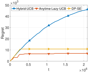
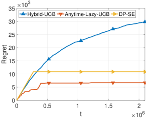
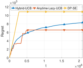
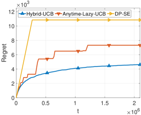
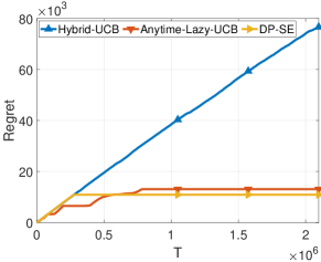
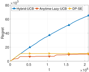
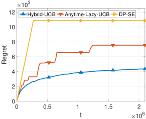
We conduct experiments to see the practical performance of Anytime-Lazy-UCB, Hybrid-UCB, and DP-SE of  Sajed & Sheffet (2019). We set $T=2\times 2^{21}$ and each plot is an average of $15$ independent runs. We set $\beta=1/T$ in DP-SE. For the choices of $\epsilon$, we set $\epsilon=0.10,0.25,0.5,1,8,64,128$. We set the number of arms $K=5$ and reuse the same mean reward settings of Sajed & Sheffet (2019):

1. Mean reward setting 1: $0.75,0.70,0.70,0.70,0.70$;

2. Mean reward setting 2: $0.75,0.625,0.5,0.375,0.25$.

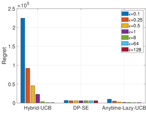
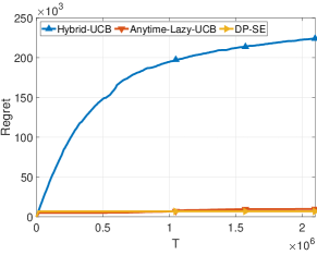
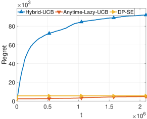
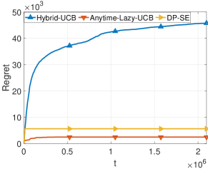
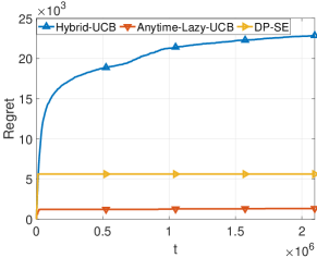
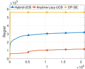
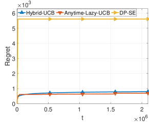
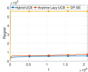
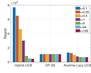
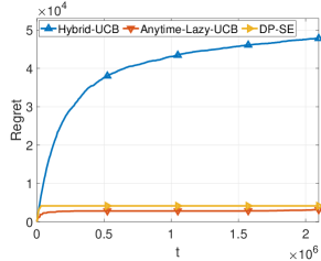
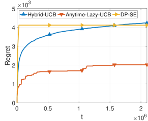
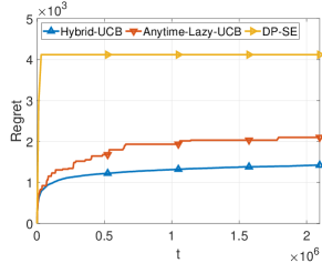
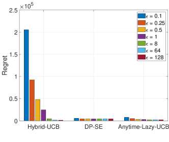
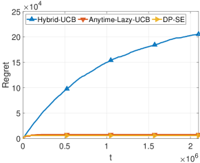
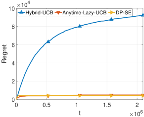
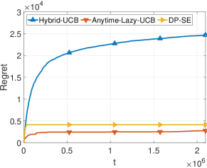
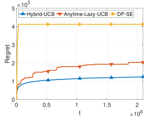
Figures 1 and 2 show that when $\epsilon$ is small ($\epsilon=0.5,1$), Anytime-Lazy-UCB is competitive with DP-SE while Hybrid-UCB does not perform well. However, when $\epsilon$ is large ($\epsilon=8,64$), Hybrid-UCB starts performing well, as shown in Figures 3 and 4. The larger $\epsilon$ is, the better the performance. This fact is just what we have expected, as Hybrid-UCB with a large $\epsilon$ value is basically UCB1 of Auer et al. (2002). Recall that Hybrid-UCB uses all the observations obtained so far to compute differentially private empirical mean and updates the differentially private empirical mean of the pulled arm at the end of each round. Figure 5 summarizes the final regret (the total regret suffered by the end of round $T$) for all the considered choices of $\epsilon$ and all the compared algorithms. Apparently, for the UCB-based algorithms, Hybrid-UCB and Anytime-Lazy-UCB, the final regret decreases as $\epsilon$ increases. However, just as already shown in (Sajed & Sheffet, 2019), the final regret of DP-SE with different choices of $\epsilon$ tends to stay flat. Figures 6, 7, and 8 show the performance of all the algorithms in mean reward setting 2 with $\epsilon=0.5,8,64$. Generally, all three algorithms in setting 2 behave very similarly to how they perform in setting 1, e.g., Anytime-Lazy-UCB is competitive with DP-SE and Hybrid-UCB performs well with large $\epsilon$ values. Appendix I provides more plots with other choices of $\epsilon$.

Figure 5: Mean reward setting 1: final regret for all $\epsilon$

Figure 6: Mean reward setting 2: regret with $\epsilon=0.5$

Figure 7: Mean reward setting 2: regret with $\epsilon=8$

Figure 8: Mean reward setting 2: regret with $\epsilon=64$

7 Conclusion

We have introduced the first non-elimination-style algorithm that obtains the optimal problem-dependent regret for differentially private stochastic bandits. Moreover, it is an anytime algorithm, a property that DP-SE (which is also optimal) does not have. While it may be possible to obtain an anytime variant of DP-SE by way of the exponential trick of Besson & Kaufmann (2018); Auer & Ortner (2010) to preserve the regret bounds, using such tricks is wasteful and may harm the regret by a multiplicative constant between 4 or 8, depending on whether the focus is to preserve problem-dependent regret bounds or problem-independent regret bounds. Despite the above difference, Anytime-Lazy-UCB and DP-SE share in common that they are both lazy and forgetful, i.e., they both update the differentially private empirical mean occasionally and use the newly obtained information only. This raises a natural open question: Is there any optimal algorithm for this setting that avoids being either lazy or forgetful?

Suppose that such an optimal algorithm exists which simultaneously avoids both of these properties. Such an algorithm would use all the history information obtained by the end of each round, in the style of classic UCB-style algorithms. We conjecture that any such algorithm cannot be optimal. Proving this would require a lower bound. We further conjecture that the lower bound is $\Omega\left(\max\left\{\frac{K\log(T)}{\Delta},\frac{K\log(T)}{\epsilon}\cdot\log\left(\frac{\log(T)}{\epsilon\cdot\Delta}\right)\right\}\right)$. Note that this conjectured lower bound matches the regret upper bound of Hybrid-UCB in Theorem 5.

In the stochastic full-information setting, there is a gap between our problem-dependent upper and lower bounds. Surprisingly, for fixed $\Delta_{\min}$ the hard instance used to prove the problem-dependent lower bound (Theorem 10) is not the instance which maximizes our upper bound (Theorem 7). Indeed, for this instance, where all suboptimal experts $j$ have $\Delta_{j}=\Delta_{\min}$, our upper bound achieves the rate $\frac{\log K}{\min\{\Delta,\epsilon\}}$, which is the same rate as our lower bound. Rather, the witness of the largest discrepancy between our upper and lower bounds is when we have the “doubling instance” $\Delta_{j}=\Delta_{\min}\cdot 2^{j-2}$ for $j=2,3,\ldots,K$ for $\varepsilon\leq\Delta_{\min}$, in which case our upper bound is of order

$$\frac{\log K}{\Delta_{\min}}+\frac{\log(K)\log(T)}{\varepsilon}.$$

Intuitively, the “doubling” instance should not be more difficult than the instance used to prove the lower bound. Therefore, we conjecture that the rate of $\frac{\log K}{\min\{\Delta_{\min},\varepsilon\}}$ is optimal. It would be very interesting to resolve the gap between the upper and lower bounds.

Supplementary material

The organization of this supplementary material is as follows:

• A - Efficient implementation of Algorithm 1

• B - Proof of Theorem 2

• C - Proof of Theorem 3

• D - Proof of Theorem 4

• E - Discussion on Hybrid mechanism-based UCB and proof of Theorem 5

• F - Proof of Theorem 6

• G - Proof of Theorem 7 (upper bound for the full-information setting)

• H - Proof of Theorem 10 (lower bound for the full-information setting)

• I - Additional experimental plots

In these sections, we will often make use of the following facts.

Fact 1. (Fact 3.7 in (Dwork et al., 2014)). If $Y\sim\text{Lap}(b)$, for any $0<\delta<1$, we have

$$\mathbb{P}\left\{|Y|>\ln\left(\frac{1}{\delta}\right)\cdot b\right\}=\delta.$$ (6)

Fact 2. (Corollary 2.9 in (Chan et al., 2011)). Let $\gamma_{1},\gamma_{2},\dotsc,\gamma_{n}$ be i.i.d. random variables drawn from $\text{Lap}(b)$. Let $Y=\sum\limits_{i=1}^{n}\gamma_{i}$. For any $0<\delta<1$, and $\chi>b\cdot\max\left\{\sqrt{n},\sqrt{\ln\left(\frac{2}{\delta}\right)}\right\}$, we have

$$\mathbb{P}\left\{|Y|>\chi\cdot\sqrt{8\ln\left(\frac{2}{\delta}\right)}\right\}\leq\delta.$$ (7)

Appendix A Efficient implementation of Algorithm 1

We can compress $\mathcal{T}_{j}^{(r)}$ to a tuple $\left(N_{j}^{(r)},S_{j}^{(r)},\lambda_{j}^{(r)}\right)$ rather than explicitly creating an array $\mathcal{T}_{j}^{(r)}$, where counter $N_{j}^{(r)}$ records the number of already inserted observations and $S_{j}^{(r)}$ records the aggregated rewards among these inserted $N_{j}^{(r)}$ observations. When $N_{j}^{(r)}$ hits $\lambda_{j}^{(r)}$, the differentially private empirical mean of arm $j$ will be updated. Note that Algorithm 1 uses two tuples simultaneously at most. Therefore, the space complexity of Anytime-Lazy-UCB is $O(K)$ if using this efficient implementation as each arm only consumes constant space.

Appendix B Proof of Theorem 2

Proof of Theorem 2:.

Let ${X}_{1:T}$ be the original reward vector sequence and ${X}^{\prime}_{1:T}$ be an arbitrary neighbouring reward vector sequence of ${X}_{1:T}$ such that they can differ in an arbitrary round. Let us say ${X}_{1:T}$ and ${X}^{\prime}_{1:T}$ differ from each other in round $t$. Let $D_{1:T}$ be the sequence of decisions made through round $1$ to round $T$ when working over ${X}_{1:T}$. Let $D_{1:T}^{\prime}$ be the sequence of decisions made when working over ${X}^{\prime}_{1:T}$.

For an arbitrary $\sigma_{1:T}\in\mathcal{A}^{T}$, we claim that

$$\mathbb{P}\left\{D_{1:T}=\sigma_{1:T}\mid X_{1:T}\right\}\leq e^{\epsilon}\cdot\mathbb{P}\left\{D_{1:T}^{\prime}=\sigma_{1:T}\mid X^{\prime}_{1:T}\right\}\quad.$$ (8)

To prove this claim, we rewrite both sides in (8) first.

The LHS in (8) can be expressed as

$$\mathbb{P}\left\{D_{1:T}=\sigma_{1:T}\mid X_{1:T}\right\}=\mathbb{P}\left\{D_{1:t}=\sigma_{1:t}\mid X_{1:T}\right\}\cdot\underbrace{\mathbb{P}\left\{D_{t+1:T}=\sigma_{t+1:T}\mid D_{1:t}=\sigma_{1:t},X_{1:T}\right\}}_{\eta}\quad.$$ (9)

Similarly, we have

$$\mathbb{P}\left\{D^{\prime}_{1:T}=\sigma_{1:T}\mid X^{\prime}_{1:T}\right\}=\mathbb{P}\left\{D^{\prime}_{1:t}=\sigma_{1:t}\mid X^{\prime}_{1:T}\right\}\cdot\underbrace{\mathbb{P}\left\{D^{\prime}_{t+1:T}=\sigma_{t+1:T}\mid D^{\prime}_{1:t}=\sigma_{1:t},X^{\prime}_{1:T}\right\}}_{\eta^{\prime}}\quad.$$ (10)

Since ${X}_{1:T}$ and ${X}^{\prime}_{1:T}$ only differ in round $t$ at most, the sequence of arms pulled up to round $t$ (including round $t$) has the same distribution either of ${X}_{1:T}$ or ${X}^{\prime}_{1:T}$. That is also to say, we have

$$\mathbb{P}\left\{D_{1:t}=\sigma_{1:t}\mid X_{1:T}\right\}=\mathbb{P}\left\{D^{\prime}_{1:t}=\sigma_{1:t}\mid X^{\prime}_{1:T}\right\}\quad.$$ (11)

We now only need to prove $\eta\leq e^{\epsilon}\cdot\eta^{\prime}$ to conclude the proof.

Let $r$ be the index of the array where the observation obtained in round $t$, i.e., $X_{J_{t}}(t)$, is inserted, when taking $X_{1:T}$ as input. Note that $r$ is random. Let $t_{*}\geq t$ be the first round such that, at the end of this round, array $\mathcal{T}_{J_{t}}^{(r)}$ is full of inserted observations. Note that $t_{*}$ is also random.

Then $\eta$ can be expressed as

$$\begin{array}[]{lll}\eta&=&\sum\limits_{j\in\mathcal{A}}\sum\limits_{q=1}^{\log(T)}\sum\limits_{s=t}^{T}\mathbb{P}\left\{J_{t}=j,r=q,t_{*}=s\mid D_{1:t}=\sigma_{1:t},X_{1:T}\right\}\\ &&\underbrace{\mathbb{P}\left\{D_{t+1:T}=\sigma_{t+1:T}\mid J_{t}=j,r=q,t_{*}=s,D_{1:t}=\sigma_{1:t},X_{1:T}\right\}}_{\alpha}\quad.\end{array}$$ (12)

Similarly, let $J^{\prime}_{t}$ be the arm pulled in round $t$ when working over ${X}^{\prime}_{1:T}$. Let $r^{\prime}$ be the index of the array where observation $X^{\prime}_{J^{\prime}_{t}}(t)$ is inserted. Let $t^{\prime}_{*}\geq t$ be the first round such that, at the end of this round, array $\mathcal{T}_{J^{\prime}_{t}}^{(r^{\prime})}$ is full of inserted observations.

Then $\eta^{\prime}$ can be expressed as

$$\begin{array}[]{lll}\eta^{\prime}&=&\sum\limits_{j\in\mathcal{A}}\sum\limits_{q=1}^{\log(T)}\sum\limits_{s=t}^{T}\mathbb{P}\left\{J^{\prime}_{t}=j,r^{\prime}=q,t^{\prime}_{*}=s\mid D^{\prime}_{1:t}=\sigma_{1:t},X^{\prime}_{1:T}\right\}\\ &&\underbrace{\mathbb{P}\left\{D^{\prime}_{t+1:T}=\sigma_{t+1:T}\mid J^{\prime}_{t}=j,r^{\prime}=q,t^{\prime}_{*}=s,D^{\prime}_{1:t}=\sigma_{1:t},X^{\prime}_{1:T}\right\}}_{\alpha^{\prime}}\quad.\end{array}$$ (13)

Since $X_{1:t-1}=X^{\prime}_{1:t-1}$, $X_{t+1:T}=X^{\prime}_{t+1:T}$, and the fact that $X_{J_{t}}(t)$ (or $X^{\prime}_{J^{\prime}_{t}}(t)$) will only be used after array $\mathcal{T}_{J_{t}}^{(r)}$ or $\mathcal{T}_{J^{\prime}_{t}}^{(r^{\prime})}$ is full of inserted observations, we have that $J_{t}$ and $J^{\prime}_{t}$ have the same distribution, $r$ and $r^{\prime}$ have the same distribution, and $t_{*}$ and $t^{\prime}_{*}$ have the same distribution. Therefore, only $\alpha$ and $\alpha^{\prime}$ are different in (12) and (13). We now show $\alpha\leq e^{\epsilon}\cdot\alpha^{\prime}$.

We now rewrite $\alpha$ as

$$\begin{array}[]{lll}\alpha&=&\mathbb{P}\left\{D_{t+1:T}=\sigma_{t+1:T}\mid J_{t}=j,r=q,t_{*}=s,D_{1:t}=\sigma_{1:t},X_{1:T}\right\}\\ &=&\mathbb{P}\left\{D_{t+1:t_{*}}=\sigma_{t+1:t_{*}}\mid J_{t}=j,r=q,t_{*}=s,D_{1:t}=\sigma_{1:t},X_{1:T}\right\}\\ &&\underbrace{\mathbb{P}\left\{D_{t_{*}+1:T}=\sigma_{t_{*}+1:T}\mid\underbrace{D_{t+1:t_{*}}=\sigma_{t+1:t_{*}},J_{t}=j,r=q,t_{*}=s,D_{1:t}=\sigma_{1:t},X_{1:T}}_{=:M}\right\}}_{\beta}\end{array}$$ (14)

Similarly, we rewrite $\alpha^{\prime}$ as

$$\begin{array}[]{lll}\alpha^{\prime}&=&\mathbb{P}\left\{D^{\prime}_{t+1:T}=\sigma_{t+1:T}\mid J^{\prime}_{t}=j,r^{\prime}=q,t^{\prime}_{*}=s,D^{\prime}_{1:t}=\sigma_{1:t},X^{\prime}_{1:T}\right\}\\ &=&\mathbb{P}\left\{D^{\prime}_{t+1:t^{\prime}_{*}}=\sigma_{t+1:t^{\prime}_{*}}\mid J^{\prime}_{t}=j,r^{\prime}=q,t^{\prime}_{*}=s,D^{\prime}_{1:t}=\sigma_{1:t},X^{\prime}_{1:T}\right\}\\ &&\underbrace{\mathbb{P}\left\{D^{\prime}_{t^{\prime}_{*}+1:T}=\sigma_{t^{\prime}_{*}+1:T}\mid\underbrace{D^{\prime}_{t+1:t^{\prime}_{*}}=\sigma_{t+1:t^{\prime}_{*}},J^{\prime}_{t}=j,r^{\prime}=q,t^{\prime}_{*}=s,D^{\prime}_{1:t}=\sigma_{1:t},X^{\prime}_{1:T}}_{=:M^{\prime}}\right\}}_{\beta^{\prime}}\end{array}$$ (15)

Since $X_{t+1:T}=X^{\prime}_{t+1:T}$, and the fact that $X_{J_{t}}(t)$ (or $X^{\prime}_{J^{\prime}_{t}}(t)$) will only be used after array $\mathcal{T}_{J_{t}}^{(r)}$ or $\mathcal{T}_{J^{\prime}_{t}}^{(r^{\prime})}$ is full of inserted observations, we have that $D_{t+1:t_{*}}$ and $D^{\prime}_{t+1:t^{\prime}_{*}}$ have the same conditional distribution. We now show $\beta\leq e^{\epsilon}\cdot\beta^{\prime}$. The key idea to prove this piece of argument is to use the property that differential privacy is immune to post-processing.

Recall that $\widetilde{\mu}_{J_{t},\lambda_{J_{t}}^{(r)},r}$ is the differentially private empirical mean of arm $J_{t}$ among all inserted observations in array $\mathcal{T}_{J_{t}}^{(r)}$ (i.e., at the end of round $t_{*}$) when working over $X_{1:T}$. Let $\widetilde{\mu}_{J^{\prime}_{t},\lambda_{J^{\prime}_{t}}^{(r^{\prime})},r^{\prime}}$ be the differentially private empirical mean of arm $J^{\prime}_{t}$ among all inserted observations in array $\mathcal{T}_{J^{\prime}_{t}}^{(r^{\prime})}$ (i.e., at the end of round $t^{\prime}_{*}$) when working over $X^{\prime}_{1:T}$.

As $\text{Lap}\left(\frac{1}{\epsilon}\right)$ noise is injected to each array after the array is full of inserted observations, for all $\mathcal{I}\subseteq\mathbb{R}$, we have

$$\begin{array}[]{ll}&\mathbb{P}\left\{\widetilde{\mu}_{J_{t},\lambda_{J_{t}}^{(r)},r}\cdot\lambda_{J_{t}}^{(r)}\in\mathcal{I}\mid M\right\}\\ \leq&e^{\epsilon}\cdot\mathbb{P}\left\{\widetilde{\mu}_{J^{\prime}_{t},\lambda_{J^{\prime}_{t}}^{(r^{\prime})},r^{\prime}}\cdot\lambda_{J^{\prime}_{t}}^{(r^{\prime})}\in\mathcal{I}\mid M^{\prime}\right\}\quad.\end{array}$$ (16)

As $X_{t_{*}+1:T}=X^{\prime}_{t^{\prime}_{*}+1:T}$, we have

$$\begin{array}[]{ll}&\mathbb{P}\left\{D_{t_{*}+1:T}=\sigma_{t_{*}+1:T}\mid\widetilde{\mu}_{J_{t},\lambda_{J_{t}}^{(r)},r}\cdot\lambda_{J_{t}}^{(r)}\in\mathcal{I},M\right\}\\ =&\mathbb{P}\left\{D^{\prime}_{t^{\prime}_{*}+1:T}=\sigma_{t^{\prime}_{*}+1:T}\mid\widetilde{\mu}_{J^{\prime}_{t},\lambda_{J^{\prime}_{t}}^{(r^{\prime})},r^{\prime}}\cdot\lambda_{J^{\prime}_{t}}^{(r^{\prime})}\in\mathcal{I},M^{\prime}\right\}\quad.\end{array}$$ (17)

By combining (16) and (17), we have $\beta\leq e^{\epsilon}\cdot\beta^{\prime}$, which concludes the proof. ∎

Appendix C Proof of Theorem 3

Proof of Theorem 3:.

To prove Theorem 3, instead of upper bounding the expected number of pulls of a sub-optimal arm $j$ directly, we take a different approach. Our new approach is based on which array the last observation of arm $j$ is inserted into. Let $\theta_{j}$ be index of the array where the $O_{j}(T)$-th observation is inserted. Note that $\theta_{j}$ is random. Let $d_{j}:=\left\lceil\log\left(\frac{24\ln(T)}{\Delta_{j}\cdot\min\{\Delta_{j},\epsilon\}}\right)\right\rceil$ and $\omega_{j}^{(r)}:=\sum\limits_{s=1}^{r}\lambda_{j}^{(s)}=\sum\limits_{s=1}^{r}2^{r}=2^{r+1}-2$. Then we have $\omega_{j}^{(d_{j})}=O\left(\frac{\log(T)}{\Delta_{j}\cdot\min\left\{\Delta_{j},\epsilon\right\}}\right)$.

We have that the number of pulls of a sub-optimal arm $j$ by the end of round $T$ (except for the pull in the initialization phase) is at most

$$\begin{array}[]{ll}O_{j}(T)&\leq\sum\limits_{r=1}^{\theta_{j}}\lambda_{j}^{(r)}=\sum\limits_{r=1}^{d_{j}}\lambda_{j}^{(r)}+\sum\limits_{r=d_{j}+1}^{\theta_{j}}\lambda_{j}^{(r)}=\omega_{j}^{(d_{j})}+\sum\limits_{r=d_{j}+1}^{\theta_{j}}\lambda_{j}^{(r)}.\end{array}$$ (18)

By taking the expectation of both sides, we have

$$\begin{array}[]{lll}\mathbb{E}\left[O_{j}(T)\right]&\leq&\mathbb{E}\left[\sum\limits_{r=1}^{\theta_{j}}\lambda_{j}^{(r)}\right]\\ &\leq&\omega_{j}^{(d_{j})}+\sum\limits_{s=d_{j}+1}^{\log(T)}\mathbb{P}\left\{\theta_{j}=s\right\}\cdot\sum\limits_{r=d_{j}+1}^{s}\lambda_{j}^{(r)}\\ &\leq&\omega_{j}^{(d_{j})}+\sum\limits_{s=d_{j}+1}^{\log(T)}\underbrace{\mathbb{P}\left\{\theta_{j}=s\right\}\cdot\omega_{j}^{(s)}}_{=O(1),\text{ Lemma\leavevmode\nobreak\ \ref{Tomorrow}}}\\ &\leq&O\left(\frac{\log(T)}{\Delta_{j}\cdot\min\left\{\Delta_{j},\epsilon\right\}}\right)+O\left(\log(T)\right)\\ &=&O\left(\frac{\log(T)}{\Delta_{j}\cdot\min\left\{\Delta_{j},\epsilon\right\}}\right)\quad.\end{array}$$ (19)

The second term in the third inequality of (19) uses the fact that $\sum\limits_{r=d_{j}+1}^{s}\lambda_{j}^{(r)}\leq\omega_{j}^{(s)}$. Also, if the last observation of arm $j$ is inserted into array $\mathcal{T}_{j}^{(s)}$, where $s\geq d_{j}+1$, it implies array $\mathcal{T}_{j}^{(s-1)}$ has no empty slots left at all, i.e., the number of inserted observations in array $\mathcal{T}_{j}^{(s-1)}$ is $\lambda_{j}^{(s-1)}=2^{s-1}\geq 2^{d_{j}+1-1}\geq\frac{24\ln(T)}{\Delta_{j}\cdot\min\{\Delta_{j},\epsilon\}}$. This amount of i.i.d. observations makes the probability that arm $j$ is pulled in the future very low. We formalize this intuition in Lemma 11.

Lemma 11.

For a fixed sub-optimal arm $j$ and $s\geq d_{j}+1$, we have $\mathbb{P}\left\{\theta_{j}=s\right\}\cdot\omega_{j}^{(s)}\leq O(1)$.

We now prove Theorem 3 and defer the proof of Lemma 11 to the end of this section.

From (2), we have the regret

$$\begin{array}[]{lll}\mathcal{R}(T)&=&\sum\limits_{j\in\mathcal{A}:\Delta_{j}>0}\mathbb{E}\left[O_{j}(T)\right]\cdot\Delta_{j}\leq\sum\limits_{j\in\mathcal{A}:\Delta_{j}>0}O\left(\frac{\log(T)}{\Delta_{j}\cdot\min\left\{\Delta_{j},\epsilon\right\}}\right)\cdot\Delta_{j}=\sum\limits_{j\in\mathcal{A}:\Delta_{j}>0}O\left(\frac{\log(T)}{\min\left\{\Delta_{j},\epsilon\right\}}\right),\end{array}$$ (20)

which concludes the proof.∎

Proof of Lemma 11:.

Recall that $d_{j}=\left\lceil\log\left(\frac{24\ln(T)}{\Delta_{j}\cdot\min(\Delta_{j},\epsilon)}\right)\right\rceil$ and $\omega_{j}^{(r)}=\sum\limits_{s=1}^{r}\lambda_{j}^{(s)}=\sum\limits_{s=1}^{r}2^{r}=2^{r+1}-2$. Then we have $\log\left(\frac{24\ln(T)}{\Delta_{j}\cdot\min(\Delta_{j},\epsilon)}\right)\leq 2^{d_{j}}\leq 2\log\left(\frac{24\ln(T)}{\Delta_{j}\cdot\min(\Delta_{j},\epsilon)}\right)$. We upper bound the LHS of Lemma 11 as

$$\begin{array}[]{ll}&\mathbb{P}\left\{\theta_{j}=s\right\}\cdot\omega_{j}^{(s)}\\ \leq&\mathbb{P}\left\{\exists t\in\{\omega_{j}^{(s-1)}+1+K,\dotsc,T\}:J_{t}=j,r_{j}(t-1)=s-1\right\}\cdot\omega_{j}^{(s)}\\ \leq&\sum\limits_{t=\omega_{j}^{(s-1)}}^{T}\mathbb{P}\left\{\overline{\mu}_{j}(t)\geq\overline{\mu}_{1}(t),r_{j}(t-1)=s-1\right\}\cdot\omega_{j}^{(s)}\\ \leq&\sum\limits_{t=\omega_{j}^{(s-1)}}^{T}\mathbb{E}\left[\bm{1}\left\{\overline{\mu}_{j}(t)\geq\overline{\mu}_{1}(t),r_{j}(t-1)=s-1\right\}\right]\cdot\omega_{j}^{(s)}\\ \leq&\sum\limits_{t=\omega_{j}^{(s-1)}}^{T}\sum\limits_{\tau=0}^{\left\lfloor\log(t)\right\rfloor-1}\mathbb{E}\left[\bm{1}\left\{\underbrace{\widetilde{\mu}_{j,2^{s-1},s-1}+\sqrt{\frac{\ln(t^{3})}{2^{s-1}}}+\frac{\ln(t^{3})}{\epsilon 2^{s-1}}\geq\widetilde{\mu}_{1,2^{\tau},\tau}+\sqrt{\frac{\ln(t^{3})}{2^{\tau}}}+\frac{\ln(t^{3})}{\epsilon 2^{\tau}}}_{\Psi}\right\}\right]\omega_{j}^{(s)}\quad.\end{array}$$ (21)

If $\Psi$ is true, then at least one of the following is true:

$$\widetilde{\mu}_{j,2^{s-1},s-1}\geq\mu_{j}+\sqrt{\frac{\ln(t^{3})}{2^{s-1}}}+\frac{\ln(t^{3})}{\epsilon 2^{s-1}}\quad;$$ (22)

$$\widetilde{\mu}_{1,2^{\tau},\tau}\leq\mu_{1}-\sqrt{\frac{\ln(t^{3})}{2^{\tau}}}-\frac{\ln(t^{3})}{\epsilon 2^{\tau}}\quad;$$ (23)

$$\frac{\Delta_{j}}{2}<\sqrt{\frac{\ln(t^{3})}{2^{s-1}}}+\frac{\ln(t^{3})}{\epsilon 2^{s-1}}\quad.$$ (24)

For (22), we apply inequality (6) and Hoeffding’s inequality. We have

$$\begin{array}[]{ll}&\mathbb{P}\left\{\widetilde{\mu}_{j,2^{s-1},s-1}\geq\mu_{j}+\sqrt{\frac{\ln(t^{3})}{2^{s-1}}}+\frac{\ln(t^{3})}{\epsilon 2^{s-1}}\right\}\\ \leq&\underbrace{\mathbb{P}\left\{\widetilde{\mu}_{j,2^{s-1},s-1}\geq\widehat{\mu}_{j,2^{s-1},s-1}+\frac{\ln(t^{3})}{\epsilon 2^{s-1}}\right\}}_{\text{Inequality (\ref{fact 1})}}+\underbrace{\mathbb{P}\left\{\widehat{\mu}_{j,2^{s-1},s-1}\geq\mu_{j}+\sqrt{\frac{\ln(t^{3})}{2^{s-1}}}\right\}}_{\text{Hoeffding's inequality}}\\ =&O\left(\frac{1}{t^{3}}\right)\quad.\end{array}$$ (25)

Similarly, for (23), we have

$$\mathbb{P}\left\{\widetilde{\mu}_{1,2^{\tau},\tau}\leq\mu_{1}-\sqrt{\frac{\ln(t^{3})}{2^{\tau}}}-\frac{\ln(t^{3})}{\epsilon 2^{\tau}}\right\}=O\left(\frac{1}{t^{3}}\right)\quad.$$ (26)

We now prove that inequality (24) cannot be true by using contradiction. The RHS in (24) is upper bounded as

$$\begin{array}[]{lll}&&\sqrt{\frac{\ln(t^{3})}{2^{s-1}}}+\frac{\ln(t^{3})}{\epsilon 2^{s-1}}\\ &\leq&\sqrt{\frac{\ln(T^{3})}{2^{d_{j}}}}+\frac{\ln(T^{3})}{\epsilon 2^{d_{j}}}\quad\text{(Note that $s-1\geq d_{j}$)}\\ &\leq&\sqrt{\frac{\ln(T^{3})}{\frac{24\ln(T)}{\Delta_{j}\cdot\min\left\{\Delta_{j},\epsilon\right\}}}}+\frac{\ln(T^{3})}{\epsilon\cdot\frac{24\ln(T)}{\Delta_{j}\cdot\min\left\{\Delta_{j},\epsilon\right\}}}\quad\text{(Use the lower bound of $2^{d_{j}}$)}\\ &<&0.5\Delta_{j}\quad,\end{array}$$ (27)

which implies that (24) cannot be true.

We now come back to (21) and have

$$\begin{array}[]{ll}&\mathbb{P}\left\{\theta_{j}=s\right\}\omega_{j}^{(s)}\\ \leq&\sum\limits_{t=\omega_{j}^{(s-1)}}^{T}\sum\limits_{\tau=0}^{\left\lfloor\log(t)\right\rfloor-1}\mathbb{E}\left[\underbrace{\bm{1}\left\{\widetilde{\mu}_{j,2^{s-1},s-1}+\sqrt{\frac{\ln(t^{3})}{2^{s-1}}}+\frac{\ln(t^{3})}{\epsilon 2^{s-1}}\geq\widetilde{\mu}_{1,2^{\tau},\tau}+\sqrt{\frac{\ln(t^{3})}{2^{\tau}}}+\frac{\ln(t^{3})}{\epsilon 2^{\tau}}\right\}}_{\Psi}\right]\omega_{j}^{(s)}\\ \leq&\sum\limits_{t=\omega_{j}^{(s-1)}}^{T}\sum\limits_{\tau=0}^{\left\lfloor\log(t)\right\rfloor-1}\left(\underbrace{\mathbb{P}\left\{\widetilde{\mu}_{j,2^{s-1},s-1}\geq\mu_{j}+\sqrt{\frac{\ln(t^{3})}{2^{s-1}}}+\frac{\ln(t^{3})}{\epsilon 2^{s-1}}\right\}}_{(=O(1/t^{3}))}+\underbrace{\mathbb{P}\left\{\widetilde{\mu}_{1,2^{\tau},\tau}\leq\mu_{1}-\sqrt{\frac{\ln(t^{3})}{2^{\tau}}}-\frac{\ln(t^{3})}{\epsilon 2^{\tau}}\right\}}_{(=O(1/t^{3}))}\right)\omega_{j}^{(s)}\\ \leq&\sum\limits_{t=\omega_{j}^{(s-1)}}^{T}\sum\limits_{\tau=0}^{\left\lfloor\log(t)\right\rfloor-1}O\left(\frac{1}{t^{3}}\right)\cdot\omega_{j}^{(s)}\\ \leq&\sum\limits_{t=\omega_{j}^{(s-1)}}^{T}O\left(\frac{1}{t^{2}}\right)\cdot\omega_{j}^{(s)}\\ \leq&\int_{\omega_{j}^{(s-1)}}^{T}O\left(\frac{1}{t^{2}}\right)d_{t}\cdot\omega_{j}^{(s)}\\ <&O\left(\frac{\omega_{j}^{(s)}}{\omega_{j}^{(s-1)}}\right)\\ \leq&O(1)\quad.\end{array}$$ (28)

The second to last inequality uses the following fact. When $r\geq 1$, we have $\frac{\omega_{j}^{(r+1)}}{\omega_{j}^{(r)}}=\frac{2^{r+2}-2}{2^{r+1}-2}=\frac{4\cdot 2^{r}-2}{2\cdot 2^{r}-2}=\frac{2\cdot 2^{r}-1}{2^{r}-1}=\frac{2\cdot 2^{r}-2+1}{2^{r}-1}=2+\frac{1}{2^{r}-1}\leq 3$. ∎

Appendix D Proof of Theorem 4

Proof of Theorem 4:.

Let $\Delta^{*}:=\sqrt{\frac{K\log(T)}{T}}$ be the critical gap threshold and, for each $j\in\mathcal{A}$, let $N_{j}:=\mathbb{E}\left[O_{j}(T)\right]$. We use the following basic decomposition of the pseudo-regret:

$$\sum_{j\in\mathcal{A}:\Delta_{j}>0}N_{j}\Delta_{j}=\sum_{j\in\mathcal{A}:\Delta_{j}\geq\Delta^{*}}N_{j}\Delta_{j}+\sum_{j\in\mathcal{A}:0<\Delta_{j}<\Delta^{*}}N_{j}\Delta_{j}\quad.$$ (29)

We now bound each summation in turn.

The first summation in (29) can be upper bounded as

$$\begin{array}[]{lll}\sum\limits_{j\in\mathcal{A}:\Delta_{j}\geq\Delta^{*}}N_{j}\Delta_{j}&=&\sum\limits_{j\in\mathcal{A}:\Delta_{j}\geq\Delta^{*}}O\left(\frac{\log(T)}{\min\{\Delta_{j},\varepsilon\}}\right)\\ &\leq&\sum\limits_{j\in\mathcal{A}:\Delta_{j}\geq\Delta^{*}}O\left(\max\left\{\frac{\log(T)}{\Delta^{*}},\frac{\log(T)}{\varepsilon}\right\}\right)\\ &\leq&O\left(K\max\left\{\frac{\log(T)}{\Delta^{*}},\frac{\log(T)}{\varepsilon}\right\}\right)\\ &\leq&O\left(\max\left\{\sqrt{KT\log(T)},\frac{K\log(T)}{\varepsilon}\right\}\right)\quad,\end{array}$$ (30)

where the first equality uses the problem-dependent regret bound of Algorithm 1.

The second summation in (29) admits the bound:

$$\sum_{j\in\mathcal{A}:0<\Delta_{j}<\Delta^{*}}N_{j}\Delta_{j}\leq\Delta^{*}\cdot\sum_{j\in\mathcal{A}:0<\Delta_{j}<\Delta^{*}}N_{j}\leq T\Delta^{*}=\sqrt{KT\log(T)}\quad.$$ (31)

Combining (30) and (31) concludes the proof.∎

Appendix E Hybrid Mechanism-based Differentially Private UCB

E.1 Discussion of Algorithm 1 in (Tossou & Dimitrakakis, 2015)

Tossou & Dimitrakakis (2015) applied the Hybrid mechanism of Chan et al. (2011) for differentially private stochastic bandits and devised the DP-UCB-Bound learning algorithm (Algorithm 1 in (Tossou & Dimitrakakis, 2015)). They claimed an $O\left(\frac{K\log(T)}{\Delta}+\frac{K\log(T)}{\epsilon}\log\left(\frac{\log(T)}{\Delta\cdot\epsilon}\right)\right)$ regret bound of their DP-UCB-Bound learning algorithm.

However, Sajed & Sheffet (2019) raised some concerns about their claimed regret bound. We carefully studied the proof of Theorem 3.2 of Tossou & Dimitrakakis (2015) and found numerous issues, e.g., (A.6), and all steps involving (A.6) such as (A.11), (A.12), (A.14) and afterwards. We do believe that it is possible to have a correct analysis for Algorithm 1 of Tossou & Dimitrakakis (2015). However, this new analysis is outside the scope of this appendix.

E.2 Our Hybrid-UCB

Input: Arm set $\mathcal{A}$ and privacy parameter $\epsilon$

Initialization:

for $j\in\mathcal{A}$ do

       Pull arm $j$ once and insert the corresponding observation into an empty array $\mathcal{F}_{j}^{(0)}$ with size 1; Set $\widetilde{\mu}_{j,1}\leftarrow\bm{\sum}\mathcal{F}_{j}^{(0)}+\text{Lap}\left(\frac{1}{0.5\epsilon}\right)$; Set $O_{j}\leftarrow 1$; Set $r_{j}\leftarrow 1$; Create an empty complete binary tree $\mathcal{B}_{j}^{(r_{j})}$ with $\lambda_{j}^{(r_{j})}\leftarrow 2^{r_{j}}$ leaf nodes and an empty array $\mathcal{F}_{j}^{(r_{j})}$ also with size $\lambda_{j}^{(r_{j})}\leftarrow 2^{r_{j}}$.

end for

for $t=K+1,K+2,\dotsc$ do

       Set $\overline{\mu}_{j}(t):=\widetilde{\mu}_{j,O_{j}}+\sqrt{\frac{3\log(t)}{O_{j}}}+\frac{6\sqrt{8}\log(t)\cdot\left\lfloor\log(O_{j}+1)\right\rfloor}{O_{j}\cdot\epsilon}$ for all $j\in\mathcal{A}$ and pull arm $J_{t}\in\mathop{\max}\limits_{j\in\mathcal{A}}\overline{\mu}_{j}(t)$; Set $O_{J_{t}}\leftarrow O_{J_{t}}+1$ and insert $X_{J_{t}}(t)$ into the left-most empty leaf node in $\mathcal{B}_{{J_{t}}}^{(r_{J_{t}})}$ and the left-most empty slot in $\mathcal{F}_{J_{t}}^{(r_{J_{t}})}$; Noisily sum all observations inserted into arrays $\left(\mathcal{F}_{J_{t}}^{(0)},\dotsc,\mathcal{F}_{J_{t}}^{(r_{J_{t}}-1)}\right)$ to have $\widetilde{F}_{J_{t},0:r_{J_{t}}-1}$ based on (32); Noisily sum all observations inserted into complete binary tree $\mathcal{B}_{J_{t}}^{(r_{J_{t}})}$ to have $\widetilde{B}_{J_{t},r_{J_{t}}}$ based on (33); Set $\widetilde{\mu}_{J_{t},O_{J_{t}}}\leftarrow\frac{\widetilde{F}_{J_{t},0:r_{J_{t}}-1}+\widetilde{B}_{J_{t},r_{J_{t}}}}{O_{J_{t}}}$ based on (34). if $O_{J_{t}}=\sum\limits_{r=0}^{r_{J_{t}}}\lambda_{J_{t}}^{(r)}$ then

             Set $r_{J_{t}}\leftarrow r_{J_{t}}+1$; Create a new empty complete binary tree $\mathcal{B}_{J_{t}}^{(r_{J_{t}})}$ with $\lambda_{J_{t}}^{(r_{J_{t}})}\leftarrow 2^{r_{J_{t}}}$ leaf nodes and a new empty array $\mathcal{F}_{J_{t}}^{(r_{J_{t}})}$ also with size $\lambda_{J_{t}}^{(r_{J_{t}})}\leftarrow 2^{r_{J_{t}}}$.

       end if

      

end for

Algorithm 4 Hybrid-UCB

For completeness, we present our own learning algorithm, Hybrid-UCB, by extending our array-based design. Algorithm 4 presents our Hybrid-UCB in detail. In Hybrid-UCB, two differentially private mechanisms are used simultaneously, just like the Hybrid mechanism of Chan et al. (2011), to track the differentially private empirical mean of each arm.

Let $O_{j}(t-1)$ be the number of observations of arm $j$ by the end of round $t-1$. Every time a new observation of arm $j$ is obtained, we insert this newly obtained observation into both an empty leaf node in a complete binary tree and an empty slot in an array (except the pull in initialization phase). Let $r_{j}(t-1)$ be the binary tree (and array) index that the $O_{j}(t-1)$-th observation was inserted into by the end of round $t-1$. Then we know that arrays $\left(\mathcal{F}_{j}^{(0)},\mathcal{F}_{j}^{(1)},\dotsc,\mathcal{F}_{j}^{(r_{j}(t-1)-1)}\right)$ will be full of inserted observations, as $\mathcal{F}_{j}^{(r)}$ and $\mathcal{B}_{j}^{(r)}$ are always holding the same observations. In Hybrid-UCB, all $O_{j}(t-1)$ observations are partitioned into two subsequences, and different subsequences will use different differential privacy mechanisms to inject noise.

The first subsequence contains the observations inserted into arrays $\left(\mathcal{F}_{j}^{(0)},\mathcal{F}_{j}^{(1)},\dotsc,\mathcal{F}_{j}^{(r_{j}(t-1)-1)}\right)$ and each array $\mathcal{F}_{j}^{(r)}$ is injected with noise $Z_{j}^{(r)}\sim\text{Lap}\left(\frac{1}{0.5\epsilon}\right)$. Then the noisy sum of all observations inserted into these arrays $\widetilde{F}_{j,0:r_{j}(t-1)-1}$ can be expressed as

$$\widetilde{F}_{j,0:r_{j}(t-1)-1}:=\sum\limits_{r=0}^{r_{j}(t-1)-1}\left(\bm{\sum}\mathcal{F}_{j}^{(r)}+Z_{j}^{(r)}\right)\quad.$$ (32)

The second subsequence contains the remaining observations, i.e., the ones inserted into binary tree $\mathcal{B}_{j}^{(r_{j}(t-1))}$. Note that according to the tree-based aggregation mechanism (Dwork et al., 2010; Chan et al., 2011), each node in binary tree $\mathcal{B}_{j}^{(r_{j}(t-1))}$ is injected with noise $Y_{j}^{(v)}\sim\text{Lap}\left(\frac{\log\left(\lambda_{j}^{(r_{j}(t-1))}\right)}{0.5\epsilon}\right)$, where $v$ is a node in complete binary tree $\mathcal{B}_{j}^{(r_{j}(t-1))}$. Node $v$ can be a leaf node or an internal node in $\mathcal{B}_{j}^{(r_{j}(t-1))}$. Note that $\log\left(\lambda_{j}^{(r_{j}(t-1))}\right)=r_{j}(t-1)$. The noisy sum of all observations inserted into the binary tree $\mathcal{B}_{j,r_{j}(t-1)}$ can be expressed as

$$\widetilde{B}_{j,r_{j}(t-1)}:=\bm{\sum}\mathcal{B}_{j}^{(r_{j}(t-1))}+\sum\limits_{v\in\mathcal{S}_{j,t-1}}Y_{j}^{(v)}\quad,$$ (33)

where $\bm{\sum}\mathcal{B}_{j}^{(r_{j}(t-1))}$ is the true aggregated values of all observations inserted into $\mathcal{B}_{j}^{(r_{j}(t-1))}$ and $\mathcal{S}_{j,t-1}$ is the set of nodes (p-sums) involved in the tree-based aggregation mechanism in order to noisily sum the values of observations inserted into complete binary tree $\mathcal{B}_{j}^{(r_{j}(t-1))}$. Note that the size of set $\mathcal{S}_{j,t-1}$ can be at most $\log\left(\lambda_{j}^{(r_{j}(t-1))}\right)=\log\left(2^{r_{j}(t-1)}\right)=r_{j}(t-1)$.

Let $\widetilde{\mu}_{j,O_{j}(t-1)}$ be the differentially private empirical of arm $j$ by the end of round $t-1$. It can be expressed as

$$\widetilde{\mu}_{j,O_{j}(t-1)}=\frac{\widetilde{F}_{j,0:r_{j}(t-1)-1}+\widetilde{B}_{j,r_{j}(t-1)}}{O_{j}(t-1)}\quad.$$ (34)

At the beginning of round $t$, for each arm $j$, we construct the upper confidence bound $\overline{\mu}_{j}(t)$ as

$$\overline{\mu}_{j}(t):=\widetilde{\mu}_{j,O_{j}(t-1)}+\sqrt{\frac{3\log(t)}{O_{j}(t-1)}}+\frac{6\sqrt{8}\cdot\log(t)\cdot\left\lfloor\log\left(O_{j}(t-1)+1\right)\right\rfloor}{\epsilon\cdot O_{j}(t-1)}\quad.$$ (35)

Then the arm with the highest $\overline{\mu}_{j}(t)$ will be pulled, i.e., $J_{t}\in\arg\mathop{\max}\limits_{j\in\mathcal{A}}\overline{\mu}_{j}(t)$.

At the end of round $t$, the observation of the pulled arm, $X_{J_{t}}(t)$, is inserted into the left-most empty slot (and the left-most leaf node) in the most recently created array (and tree). If there is no empty space left after inserting $X_{J_{t}}(t)$, we will create a new empty array and a new empty binary tree for future use.

E.3 Proof of Theorem 5

E.3.1 Differential privacy analysis

As Hybrid-UCB is the composition of our array-based learning algorithm, Algorithm 1 with the required privacy parameter set to $0.5\epsilon$, and the tree-based aggregation mechanism of Dwork et al. (2010); Chan et al. (2011) with the required privacy parameter set to $0.5\epsilon$, from the composition theorem of Dwork et al. (2014) (the property that $\epsilon$’s can be added up), we immediately conclude that Algorithm 4 preserves $\epsilon$-differential privacy.

E.3.2 Regret analysis

Regret bound proof of Theorem 5:.

Before we step into the detailed proof, we first give a few definitions and then we decompose the regret. Let $d_{j}:=\left\lceil\log\left(\max\left\{\frac{256\log(T)}{\Delta_{j}^{2}},\frac{256\log(T)}{\epsilon\cdot\Delta_{j}}\cdot\log\left(\frac{256\log(T)}{\epsilon\cdot\Delta_{j}}\right)\right\}\right)\right\rceil$. Let $\omega_{j}^{(r)}:=\sum\limits_{s=0}^{r}\lambda_{j}^{(r)}=\sum\limits_{s=0}^{r}2^{r}=2^{r+1}-1$. Then we have $\omega_{j}^{(d_{j})}=O\left(\max\left\{\frac{\log(T)}{\Delta_{j}^{2}},\frac{\log(T)}{\epsilon\cdot\Delta_{j}}\cdot\log\left(\frac{\log(T)}{\epsilon\cdot\Delta_{j}}\right)\right\}\right)$. Let $\theta_{j}$ be the array/tree index that the $O_{j}(T)$-th observation of arm $j$ is inserted into by the end of round $T$. Note that $\theta_{j}$ is random. Then we have the number of pulls of a sub-optimal arm $j$ by the end of round $T$ is at most

$$\begin{array}[]{lll}O_{j}(T)&\leq&\sum\limits_{r=0}^{\theta_{j}}\lambda_{j}^{(r)}\\ &=&\sum\limits_{r=0}^{d_{j}}\lambda_{j}^{(r)}+\sum\limits_{r=d_{j}+1}^{\theta_{j}}\lambda_{j}^{(r)}\\ &=&\omega_{j}^{(d_{j})}+\sum\limits_{r=d_{j}+1}^{\theta_{j}}\lambda_{j}^{(r)}\quad.\end{array}$$ (36)

As $\theta_{j}$ is random, by taking the expectation of both sides, we have

$$\begin{array}[]{lll}\mathbb{E}\left[O_{j}(T)\right]&\leq&\omega_{j}^{(d_{j})}+\mathbb{E}\left[\sum\limits_{r=d_{j}+1}^{\theta_{j}}\lambda_{j}^{(r)}\right]\\ &\leq&\omega_{j}^{(d_{j})}+\sum\limits_{s=d_{j}+1}^{\log(T)}\underbrace{\mathbb{P}\left\{\theta_{j}=s\right\}\cdot\omega_{j}^{(s)}}_{\text{Lemma}\leavevmode\nobreak\ \ref{bubble tea}}\quad.\end{array}$$ (37)

To upper bound (37), we introduce Lemma 12 first, which states that after a sub-optimal $j$ has been observed “enough” times, the probability that it will be pulled again is very low.

Lemma 12.

For a fixed sub-optimal arm $j$ and $s\geq d_{j}+1$, we have $\mathbb{P}\left\{\theta_{j}=s\right\}\cdot\omega_{j}^{(s)}=O(1)$.

We now prove Theorem 5. The proof of Lemma 12 is deferred to the end of this section.

From (2), we have

$$\begin{array}[]{lll}\mathcal{R}(T)&=&\sum\limits_{j\in\mathcal{A}:\Delta_{j}>0}\mathbb{E}\left[O_{j}(T)\right]\cdot\Delta_{j}\\ &\leq&\sum\limits_{j\in\mathcal{A}:\Delta_{j}>0}\left(\omega_{j}^{(d_{j})}\cdot\Delta_{j}+\sum\limits_{s=d_{j}+1}^{\log(T)}\underbrace{\mathbb{P}\left\{\theta_{j}=s\right\}\cdot\omega_{j}^{(s)}}_{=O(1),\ \text{Lemma\leavevmode\nobreak\ \ref{bubble tea}}}\cdot\Delta_{j}\right)\\ &=&\sum\limits_{j\in\mathcal{A}:\Delta_{j}>0}O\left(\max\left\{\frac{\log(T)}{\Delta_{j}},\frac{\log(T)}{\epsilon}\cdot\log\left(\frac{\log(T)}{\epsilon\cdot\Delta_{j}}\right)\right\}\right)\quad,\end{array}$$ (38)

which concludes the proof. ∎

Proof of Lemma 12:.

The idea behind the proof uses the fact that if the last observation of arm $j$ in inserted into array $\mathcal{F}_{j}^{(s)}$ (tree $\mathcal{B}_{j}^{(s)}$), it implies that arm $j$ is pulled again after it has already been pulled $\omega_{j}^{(s-1)}$ times. To calculate the differentially private empirical mean of these $\omega_{j}^{(s-1)}$ observations, Hybrid-UCB uses observations inserted into arrays $\left(\mathcal{F}_{j}^{(0)},\mathcal{F}_{j}^{(1)},\dotsc,\mathcal{F}_{j}^{(s-2)}\right)$ and observations inserted into $\mathcal{B}_{j}^{(s-1)}$. Note that based on our learning algorithm, all arrays $\left(\mathcal{F}_{j}^{(0)},\mathcal{F}_{j}^{(1)},\dotsc,\mathcal{F}_{j}^{(s-2)}\right)$ and binary tree $\mathcal{B}_{j}^{(s-1)}$ are full of inserted observations.

We now start the proof of Lemma 12. We have

$$\begin{array}[]{ll}&\mathbb{P}\left\{\theta_{j}=s\right\}\cdot\omega_{j}^{(s)}\\ \leq&\mathbb{P}\left\{\exists t\in\{\omega_{j}^{(s-1)}+K,\dotsc,T\}:J_{t}=j,O_{j}(t-1)=\omega_{j}^{(s-1)}\right\}\cdot\omega_{j}^{(s)}\\ \leq&\sum\limits_{t=\omega_{j}^{(s-1)}}^{T}\mathbb{E}\left[\bm{1}\left\{\overline{\mu}_{j}(t)\geq\overline{\mu}_{1}(t),O_{j}(t-1)=\omega_{j}^{(s-1)}\right\}\right]\cdot\omega_{j}^{(s)}\\ \leq&\sum\limits_{t=\omega_{j}^{(s-1)}}^{T}\sum\limits_{h=1}^{t-1}\mathbb{E}\left[\bm{1}\left\{\underbrace{\widetilde{\mu}_{j,\omega_{j}^{(s-1)}}+\sqrt{\frac{3\log(t)}{\omega_{j}^{(s-1)}}}+\frac{6\sqrt{8}\log(t)\cdot s}{\epsilon\cdot\omega_{j}^{(s-1)}}\geq\widetilde{\mu}_{1,h}+\sqrt{\frac{3\log(t)}{h}}+\frac{6\sqrt{8}\log(t)\left(\left\lfloor\log\left(h+1\right)\right\rfloor\right)}{\epsilon\cdot h}}_{\Psi}\right\}\right]\omega_{j}^{(s)}\\ \end{array}$$ (39)

If $\Psi$ is true, then at least one of the following is true:

$$\begin{array}[]{l}\widetilde{\mu}_{j,\omega_{j}^{(s-1)}}\geq\mu_{j}+\sqrt{\frac{3\log(t)}{\omega_{j}^{(s-1)}}}+\frac{6\sqrt{8}\log(t)\cdot s}{\epsilon\cdot\omega_{j}^{(s-1)}}\quad;\end{array}$$ (40)

$$\begin{array}[]{l}\widetilde{\mu}_{1,h}\leq\mu_{1}-\sqrt{\frac{3\log(t)}{h}}-\frac{6\sqrt{8}\log(t)\left(\left\lfloor\log\left(h+1\right)\right\rfloor\right)}{\epsilon\cdot h}\quad;\end{array}$$ (41)

$$\begin{array}[]{l}\frac{\Delta_{j}}{2}<\sqrt{\frac{3\log(t)}{\omega_{j}^{(s-1)}}}+\frac{6\sqrt{8}\log(t)\cdot s}{\epsilon\cdot\omega_{j}^{(s-1)}}\quad.\end{array}$$ (42)

Before we start upper bounding $\Psi$, let us first introduce some notation. Let $\widehat{F}_{j,0:r_{j}(t-1)-1}:=\sum\limits_{r=0}^{r_{j}(t-1)-1}\bm{\sum}\mathcal{F}_{j}^{(r)}$ be the aggregated reward of all observations inserted into arrays $\left(\mathcal{F}_{j}^{(0)},\mathcal{F}_{j}^{(1)},\dotsc,\mathcal{F}_{j}^{(r_{j}(t-1)-1)}\right)$, i.e., the non-noisy version of $\widetilde{F}_{j,0:r_{j}(t-1)-1}$. Similarly, let $\widehat{B}_{j,r_{j}(t-1)}=\bm{\sum}\mathcal{B}_{j}^{(r_{j}(t-1))}$ be the non-noisy version of $\widetilde{B}_{j,r_{j}(t-1)}$. Also, let $\widehat{\mu}_{j,O_{j}(t-1)}=\frac{\widehat{F}_{j,0:r_{j}(t-1)-1}+\widehat{B}_{j,r_{j}(t-1)}}{O_{j}(t-1)}$ be the true empirical mean of all these $O_{j}(t-1)$ observations, i.e., the non-noisy version of $\widetilde{\mu}_{j,O_{j}(t-1)}$. After these preparations, we now analyze (40), (41), and (42) one by one.

For (40), we use Hoeffding’s inequality and inequality (7). We have

$$\begin{array}[]{ll}&\mathbb{P}\left\{\widetilde{\mu}_{j,\omega_{j}^{(s-1)}}\geq\mu_{j}+\sqrt{\frac{3\log(t)}{\omega_{j}^{(s-1)}}}+\frac{6\sqrt{8}\log(t)\cdot s}{\epsilon\cdot\omega_{j}^{(s-1)}}\right\}\\ \leq&\mathbb{P}\left\{\widehat{\mu}_{j,\omega_{j}^{(s-1)}}\geq\mu_{j}+\sqrt{\frac{3\log(t)}{\omega_{j}^{(s-1)}}}\right\}+\mathbb{P}\left\{\widetilde{\mu}_{j,\omega_{j}^{(s-1)}}\geq\widehat{\mu}_{j,\omega_{j}^{(s-1)}}+\frac{6\sqrt{8}\log(t)\cdot s}{\epsilon\cdot\omega_{j}^{(s-1)}}\right\}\\ \leq&\mathbb{P}\left\{\widehat{\mu}_{j,\omega_{j}^{(s-1)}}\geq\mu_{j}+\sqrt{\frac{3\log(t)}{\omega_{j}^{(s-1)}}}\right\}+\mathbb{P}\left\{\widetilde{F}_{j,0:s-2}\geq\widehat{F}_{j,0:s-2}+\frac{3\sqrt{8}\log(t)\cdot s}{0.5\epsilon}\right\}+\mathbb{P}\left\{\widetilde{B}_{j,s-1}\geq\widehat{B}_{j,s-1}+\frac{3\sqrt{8}\log(t)\cdot s}{0.5\epsilon}\right\}\\ \leq&\mathbb{P}\left\{\widehat{\mu}_{j,\omega_{j}^{(s-1)}}\geq\mu_{j}+\sqrt{\frac{4\ln(t)}{\omega_{j}^{(s-1)}}}\right\}+\mathbb{P}\left\{\widetilde{F}_{j,0:s-2}\geq\widehat{F}_{j,0:s-2}+\frac{3\sqrt{8}\log(t)\cdot(s-1)}{0.5\epsilon}\right\}+\mathbb{P}\left\{\widetilde{B}_{j,s-1}\geq\widehat{B}_{j,s-1}+\frac{3\sqrt{8}\log(t)\cdot(s-1)}{0.5\epsilon}\right\}\\ =&O\left(\frac{1}{t^{4}}\right)\quad.\end{array}$$ (43)

In the last inequality of (43), for the first term, we use Hoeffding’s inequality. Note that $3\log(t)>4\ln(t)$. We now provide more details about how to apply inequality (7) for the second and the third terms. For the second term, we set $\chi=\frac{1}{0.5\epsilon}\cdot\frac{\sqrt{8}\log(t^{3})(s-1)}{\sqrt{8\ln(t^{4})}}=\frac{1}{0.5\epsilon}\cdot\frac{3\sqrt{\ln(t)}\cdot(s-1)}{2\ln(2)}>\frac{1}{0.5\epsilon}\cdot 2\sqrt{\ln(t)}(s-1)>\frac{1}{0.5\epsilon}\max\left\{\sqrt{s-1},\sqrt{\ln(t^{4})}\right\}$. For the third term, we set $\chi=\frac{s-1}{0.5\epsilon}\cdot\frac{\sqrt{8}\log(t^{3})}{\sqrt{8\ln(t^{4})}}>\frac{s-1}{0.5\epsilon}\cdot\sqrt{4\ln(t)}=\frac{s-1}{0.5\epsilon}\max\left\{\sqrt{s-1},\sqrt{\ln(t^{4})}\right\}$. Note that we always have $s-1<\log(2^{s}-1)<\log(t)<\ln(t^{4})$.

Similarly, for (41), we have

$$\begin{array}[]{l}\mathbb{P}\left\{\widetilde{\mu}_{1,h}\leq\mu_{1}-\sqrt{\frac{3\log(t)}{h}}-\frac{6\sqrt{8}\log(t)\left(\left\lfloor\log\left(h+1\right)\right\rfloor\right)}{\epsilon\cdot h}\right\}=O\left(\frac{1}{t^{4}}\right)\quad.\end{array}$$ (44)

We now show that (42) cannot be true by using contradiction. As $2^{d_{j}}\geq\max\left\{\frac{256\log(T)}{\Delta_{j}^{2}},\frac{256\log(T)}{\epsilon\cdot\Delta_{j}}\cdot\log\left(\frac{256\log(T)}{\epsilon\cdot\Delta_{j}}\right)\right\}\geq\frac{256\log(T)}{\Delta_{j}^{2}}$, the first term of the RHS in (42) is upper bounded as

$$\begin{array}[]{l}\sqrt{\frac{3\log(t)}{\omega_{j}^{(s-1)}}}<\sqrt{\frac{3\log(T)}{\lambda_{j}^{(s-1)}}}=\sqrt{\frac{3\log(T)}{2^{s-1}}}\leq\sqrt{\frac{3\log(T)}{2^{d_{j}+1-1}}}\leq\sqrt{\frac{3\log(T)}{\frac{256\log(T)}{\Delta_{j}^{2}}}}=\sqrt{\frac{3}{256}}\Delta_{j}=\frac{\sqrt{3}\Delta_{j}}{16}\quad.\end{array}$$ (45)

To upper bound the second term in the RHS of (42), we construct the following decreasing function first. Let $f(x)=\frac{x}{2^{x}}$, where $x\geq 2$. Then we have $f^{\prime}(x)=\frac{1}{2^{x}}-\frac{x\ln(2)}{2^{x}}<0$. Let $z_{j}:=\log\left(\frac{256\log(T)}{\epsilon\cdot\Delta_{j}}\cdot\log\left(\frac{256\log(T)}{\epsilon\cdot\Delta_{j}}\right)\right)$. Then we have $s\geq d_{j}+1\geq z_{j}+1>z_{j}$. Therefore, we also have

$$\frac{s}{2^{s}}<\frac{z_{j}}{2^{z_{j}}}=\frac{\log\left(\frac{256\log(T)}{\epsilon\cdot\Delta_{j}}\cdot\log\left(\frac{256\log(T)}{\epsilon\cdot\Delta_{j}}\right)\right)}{2^{\log\left(\frac{256\log(T)}{\epsilon\cdot\Delta_{j}}\cdot\log\left(\frac{256\log(T)}{\epsilon\cdot\Delta_{j}}\right)\right)}}\leq\frac{2\log\left(\frac{256\log(T)}{\epsilon\cdot\Delta_{j}}\right)}{\frac{256\log(T)}{\epsilon\cdot\Delta_{j}}\cdot\log\left(\frac{256\log(T)}{\epsilon\cdot\Delta_{j}}\right)}=\frac{\epsilon\cdot\Delta_{j}}{128\log(T)}\quad.$$ (46)

The second term in the RHS of (42) is upper bounded as

$$\frac{6\sqrt{8}\log(t)\cdot s}{\epsilon\cdot\omega_{j}^{(s-1)}}<\frac{6\sqrt{8}\log(t)\cdot s}{\epsilon\cdot\lambda_{j}^{(s-1)}}=\frac{2\cdot 6\sqrt{8}\log(t)}{\epsilon}\cdot\frac{s}{2^{s}}\leq\frac{12\sqrt{8}\log(T)}{\epsilon}\cdot\frac{\epsilon\cdot\Delta_{j}}{128\log(T)}=\frac{3\sqrt{2}\Delta_{j}}{16}\quad.$$ (47)

From (45) and (47), we know that the RHS in (42) is at most $\frac{\sqrt{3}\Delta_{j}}{16}+\frac{3\sqrt{2}\Delta_{j}}{16}<\frac{\Delta_{j}}{2}$, which implies (42) cannot be true.

We now come back to (39). We have

$$\begin{array}[]{ll}&\mathbb{P}\left\{\theta_{j}=s\right\}\cdot\omega_{j}^{(s)}\\ \leq&\sum\limits_{t=\omega_{j}^{(s-1)}}^{T}\sum\limits_{h=1}^{t-1}\mathbb{E}\left[\bm{1}\left\{\underbrace{\widetilde{\mu}_{j,\omega_{j}^{(s-1)}}+\sqrt{\frac{3\log(t)}{\omega_{j}^{(s-1)}}}+\frac{6\sqrt{8}\log(t)\cdot s}{\epsilon\cdot\omega_{j}^{(s-1)}}\geq\widetilde{\mu}_{1,h}+\sqrt{\frac{3\log(t)}{h}}+\frac{6\sqrt{8}\log(t)\left(\left\lfloor\log\left(h+1\right)\right\rfloor\right)}{\epsilon\cdot h}}_{\Psi}\right\}\right]\omega_{j}^{(s)}\\ \leq&\sum\limits_{t=\omega_{j}^{(s-1)}}^{T}\sum\limits_{h=1}^{t-1}\left(\mathbb{P}\left\{(\ref{turnlock 1})\right\}+\mathbb{P}\left\{(\ref{turnlock 2})\right\}\right)\cdot\omega_{j}^{(s)}\\ \leq&\sum\limits_{t=\omega_{j}^{(s-1)}}^{T}\sum\limits_{h=1}^{t-1}O\left(\frac{1}{t^{4}}\right)\cdot\omega_{j}^{(s)}\\ \leq&\sum\limits_{t=\omega_{j}^{(s-1)}}^{T}O\left(\frac{1}{t^{3}}\right)\cdot\omega_{j}^{(s)}\\ \leq&O\left(\frac{\omega_{j}^{(s)}}{\omega_{j}^{(s-1)}}\right)\\ \leq&O(1)\quad.\end{array}$$ (48)

Note that $\frac{\omega_{j}^{(s)}}{\omega_{j}^{(s-1)}}=\frac{2^{s+1}-1}{2^{s}-1}\leq 4$.∎

Appendix F Proof of Theorem 6

Proof of Theorem 6:.

Let $\bm{X}_{1:T}$ be the original reward vector sequence and $\bm{X}^{\prime}_{1:T}$ be an arbitrary neighbouring reward vector sequence of $\bm{X}_{1:T}$ such that they differ in an arbitrary reward vector from each other at most. Let us say they differ in the reward vector in round $t$. Let $D_{1:T}$ be the sequence of decisions made through round $1$ to $T$ when taking $\bm{X}_{1:T}$ as input. Similarly, let $D_{1:T}^{\prime}$ be the sequence of decisions made when taking $\bm{X}^{\prime}_{1:T}$ as input.

Let $\sigma_{1:T}\in\mathcal{A}^{T}$. We claim that

$$\mathbb{P}\left\{D_{1:T}=\sigma_{1:T}\mid X_{1:T}\right\}\leq e^{\epsilon}\cdot\mathbb{P}\left\{D_{1:T}^{\prime}=\sigma_{1:T}\mid X^{\prime}_{1:T}\right\}\quad.$$ (49)

Let $\tau^{(r)}$ be the last round of epoch $r$, i.e., at the end of round $\tau^{(r)}$, a new action will be output by RNM. Also, let $r_{0}$ be the epoch including round $t$. Hence, we have $t\in\left\{\tau^{(r_{0}-1)}+1,\tau^{(r_{0}-1)}+2,\dotsc,\tau^{(r_{0})}\right\}$. We set $\tau^{(0)}=0$. Note that for a fixed $t$, $r_{0}$ is also fixed.

The LHS of (49) can be rewritten as

$$\begin{array}[]{lll}\mathbb{P}\left\{D_{1:T}=\sigma_{1:T}\right\}&=&\mathop{\Pi}\limits_{1\leq r\leq r_{0}}\mathbb{P}\left\{D_{\tau^{(r-1)}+1:\tau^{(r)}}=\sigma_{\tau^{(r-1)}+1:\tau^{(r)}}\right\}\cdot\underbrace{\mathbb{P}\left\{D_{\tau^{(r_{0})}+1:\tau^{(r_{0}+1)}}=\sigma_{\tau^{(r_{0})}+1:\tau^{(r_{0}+1)}}\right\}}_{\alpha}\\ &&\mathop{\Pi}\limits_{r\geq r_{0}+2}\mathbb{P}\left\{D_{\tau^{(r-1)}+1:\tau^{(r)}}=\sigma_{\tau^{(r-1)}+1:\tau^{(r)}}\right\}\quad.\end{array}$$ (50)

Similarly, the RHS of (49) can be rewritten as

$$\begin{array}[]{lll}\mathbb{P}\left\{D^{\prime}_{1:T}=\sigma_{1:T}\right\}&=&\mathop{\Pi}\limits_{1\leq r\leq r_{0}}\mathbb{P}\left\{D^{\prime}_{\tau^{(r-1)}+1:\tau^{(r)}}=\sigma_{\tau^{(r-1)}+1:\tau^{(r)}}\right\}\cdot\underbrace{\mathbb{P}\left\{D^{\prime}_{\tau^{(r_{0})}+1:\tau^{(r_{0}+1)}}=\sigma_{\tau^{(r_{0})}+1:\tau^{(r_{0}+1)}}\right\}}_{\alpha^{\prime}}\\ &&\mathop{\Pi}\limits_{r\geq r_{0}+2}\mathbb{P}\left\{D^{\prime}_{\tau^{(r-1)}+1:\tau^{(r)}}=\sigma_{\tau^{(r-1)}+1:\tau^{(r)}}\right\}\quad.\end{array}$$ (51)

The idea behind (50) and (51) is that the decisions made in epoch $r$ only depends on the reward vector sequence in epoch $r-1$, i.e., the decisions made in epoch $r$ have no dependency on the decisions made in epoch $r-1$.

Since $\bm{X}_{1:T}$ and $\bm{X}^{\prime}_{1:T}$ only differ in round $t$ at most, the decisions made from round $1$ to round $\tau^{(r_{0})}$ (including round $\tau^{(r_{0})}$) and from round $\tau^{(r_{0}+1)}+1$ to the end stay the same under either $\bm{X}_{1:T}$ or $\bm{X}^{\prime}_{1:T}$ conditioning on the noise injected. Therefore, in (50) and (51), only $\alpha$ and $\alpha^{\prime}$ can be different. Now we analyze the relationship of $\alpha$ and $\alpha^{\prime}$.

Recall that $J^{(r)}$ indicates the action output by RNM at the end of epoch $r$ over $\bm{X}_{1:T}$. Let $J^{\prime(r)}$ indicate the action output by RNM at the end of epoch $r$ over $\bm{X}^{\prime}_{1:T}$. As $\text{Lap}\left(\frac{1}{\epsilon}\right)$ noise is injected to each action $j$’s fresh observations obtained in epoch $r_{0}$, from Claim 3.9 of (Dwork et al., 2014), we have

$$\mathbb{P}\left\{J^{(r_{0})}=\sigma_{\tau^{(r_{0})}+1}\right\}\leq e^{\epsilon}\cdot\mathbb{P}\left\{J^{\prime(r_{0})}=\sigma_{\tau^{(r_{0})}+1}\right\}\quad,$$ (52)

which implies

$$\mathbb{P}\left\{D_{\tau^{(r_{0})}+1}=\sigma_{\tau^{(r_{0})}+1}\right\}\leq e^{\epsilon}\cdot\mathbb{P}\left\{D^{\prime}_{\tau^{(r_{0})}+1}=\sigma_{\tau^{(r_{0})}+1}\right\}\quad.$$ (53)

As the decisions made in rounds $\left\{\tau^{(r_{0})}+1,\tau^{(r_{0})}+2,\dotsc,\tau^{(r_{0}+1)}\right\}$ stay the same, we have

$$\begin{array}[]{ll}&\mathbb{P}\left\{D_{\tau^{(r_{0})}+1:\tau^{(r_{0}+1)}}=\sigma_{\tau^{(r_{0})}+1:\tau^{(r_{0}+1)}}\mid D_{\tau^{(r_{0})}+1}=\sigma_{\tau^{(r_{0})}+1}\right\}\\ =&\mathbb{P}\left\{D^{\prime}_{\tau^{(r_{0})}+1:\tau^{(r_{0}+1)}}=\sigma_{\tau^{(r_{0})}+1:\tau^{(r_{0}+1)}}\mid D^{\prime}_{\tau^{(r_{0})}+1}=\sigma_{\tau^{(r_{0})}+1}\right\}\quad.\end{array}$$ (54)

By combining (53) and (54), we have $\alpha\leq e^{\epsilon}\alpha^{\prime}$, which concludes the proof.∎

Appendix G Proofs for upper bounds for the full-information setting

For our analysis, we first re-express FTNL using a convenient cumulative reward (or gain) notation. Let $G^{(r)}_{j}$ denote the cumulative reward of expert $j$ from the $2^{r}$ rounds in epoch $r$, with the convention that $G^{(-1)}_{j}=0$ for all $j\in[K]$. In addition, let $\tilde{G}_{j}^{(r)}$ be the corresponding noisy cumulative reward, defined as the sum of $G_{j}^{(r)}$ and an independent, zero-mean Laplace noise random variable with the scale parameter $b$ set as $b=1/\varepsilon$. Using this notation, at the start of any epoch $r\geq 1$, FTNL plays the expert $j$ for which $\tilde{G}_{j}^{(r-1)}$ is maximized. Also, recall from Algorithm 2 that FTNL plays expert 1 in epoch 0.

The proof of Theorem 7 makes use of the following concentration result for FTNL.

Lemma 13.

For all $r\geq r_{0}$, $k\geq 1$, and $j\in\mathcal{J}_{k}$, it holds that

$$\Pr\left(\tilde{G}_{j}^{(r)}-\tilde{G}_{1}^{(r)}\geq 0\right)\leq 2e^{-2^{r}\Delta_{(k)}\min\{\Delta_{(k)},\varepsilon\}/8}.$$

Proof.

We begin with the observation that

$$\tilde{G}_{j}^{(r)}-\tilde{G}_{1}^{(r)}=G_{j}^{(r)}-G_{1}^{(r)}+\xi_{j,r},$$

where $\xi_{j,r}$ is the sum of two independent Laplace noise random variables each with their scale parameter set to $1/\varepsilon$.

Clearly, we have

$$\Pr\left(\tilde{G}_{j}^{(r)}-\tilde{G}_{1}^{(r)}\geq 0\right) =\Pr\left(\tilde{G}_{j}^{(r)}-\tilde{G}_{1}^{(r)}+2^{r}\Delta_{j}\geq 2^{r}\Delta_{j}\right)$$

$$\leq\Pr\left(G_{j}^{(r)}-G_{1}^{(r)}+2^{r}\Delta_{j}\geq 2^{r}\Delta_{j}/2\right)+\Pr\left(\xi_{j,r}\geq 2^{r}\Delta_{j}/2\right).$$ (55)

Next, we observe that $\Delta_{j}\geq\Delta_{(k)}=2^{k-1}\Delta_{\min}$ for all $j\in\mathcal{J}_{k}$. From Hoeffding’s inequality, the first term of (55) is at most

$$e^{-2^{r}\Delta_{j}^{2}/8}\leq e^{-2^{r}\Delta_{(k)}^{2}/8}.$$

For the second term of (55), we just naively use a union bound; letting $Z$ be a Laplace random variable with scale parameter set to $1/\varepsilon$, we have

$$\Pr\left(\xi_{j,r}\geq 2^{r-1}\Delta_{j}\right)\leq 2\Pr\left(Z\geq 2^{r-2}\Delta_{j}\right)\leq e^{-\varepsilon 2^{r-2}\Delta_{j}}\leq e^{-\varepsilon 2^{r-2}\Delta_{(k)}},$$

where we can drop the factor of 2 in the penultimate step because we only need a bound on the upper tail of $Z$.

Applying the above gives

$$\Pr\left(\tilde{G}_{j}^{(r)}-\tilde{G}_{1}^{(r)}\geq 0\right) \leq e^{-2^{r}\Delta_{(k)}^{2}/8}+e^{-2^{r}\Delta_{(k)}\varepsilon/4}$$

$$\leq 2e^{-2^{r}\Delta_{(k)}\min\{\Delta_{(k)},\varepsilon\}/8}.$$

∎

Proof (of Theorem 7).

Observe that all plays of experts $j$ for which $\Delta_{j}\leq\frac{1}{T}$ can collectively contribute at most 1 to the regret, and hence it is safe to assume (ignoring experts as necessary) that $\Delta_{\min}>\frac{1}{T}$. In other words, without loss of generality, we assume all the mean reward gaps are lower bounded by $\frac{1}{T}$.

Since the pseudo-regret is non-decreasing in $T$, it is without loss of generality that we increase $T$ if necessary so that $T=2^{R+1}-1$ for some nonnegative integer $R$. Let $\tau(r):=2^{r}$ for any $r\geq 0$. Then the pseudo-regret of FTNL can be written as

$$\sum_{t=1}^{T}\sum_{j=2}^{K}\Pr(i_{t}=j)\cdot\Delta_{j} =\sum_{r=0}^{R}2^{r}\sum_{j=2}^{K}\Pr(i_{\tau(r)}=j)\cdot\Delta_{j}$$

$$=\sum_{k\geq 1}\sum_{r=0}^{R}2^{r}\sum_{j\in\mathcal{J}_{k}}\Pr(i_{\tau(r)}=j)\cdot\Delta_{j}.$$

We will bound the summation over $r$ in the last line above separately for each possible value of $k$:

$$\sum_{r=0}^{R}2^{r}\sum_{j\in\mathcal{J}_{k}}\Pr\left(i_{\tau(r)}=j\right)\cdot\Delta_{j}\leq 2^{k}\Delta_{\min}\cdot\sum_{r=0}^{R}2^{r}\sum_{j\in\mathcal{J}_{k}}\Pr\left(i_{\tau(r)}=j\right).$$

Now, observe that for any $r_{0}\geq 0$,

$$\sum_{r=0}^{R}2^{r}\Pr\left(i_{\tau(r)}\in\mathcal{J}_{k}\right)$$

$$\leq\sum_{r=0}^{R}2^{r}\Pr\left(\exists j\in\mathcal{J}_{k}\colon\tilde{G}^{(r-1)}_{j}-\tilde{G}^{(r-1)}_{1}\geq 0\right)$$

$$=\sum_{r=0}^{r_{0}}2^{r}\Pr\left(\exists j\in\mathcal{J}_{k}\colon\tilde{G}^{(r-1)}_{j}-\tilde{G}^{(r-1)}_{1}\geq 0\right)+\sum_{r=r_{0}+1}^{R}2^{r}\Pr\left(\exists j\in\mathcal{J}_{k}\colon\tilde{G}^{(r-1)}_{j}-\tilde{G}_{1}^{(r-1)}\geq 0\right)$$

$$<2^{r_{0}+1}+\sum_{r=r_{0}+1}^{\infty}2^{r}\Pr\left(\exists j\in\mathcal{J}_{k}\colon\tilde{G}_{j}^{(r-1)}-\tilde{G}_{1}^{(r-1)}\geq 0\right)$$

$$\leq 2^{r_{0}+1}+2|\mathcal{J}_{k}|\max_{j\in\mathcal{J}_{k}}\sum_{r=r_{0}}^{\infty}2^{r}\Pr\left(\tilde{G}_{j}^{(r)}-\tilde{G}_{1}^{(r)}\geq 0\right)$$

$$\leq 2^{r_{0}+1}+4|\mathcal{J}_{k}|\max_{j\in\mathcal{J}_{k}}\sum_{r=r_{0}}^{\infty}2^{r}e^{-2^{r}\Delta_{(k)}\min\{\Delta_{(k)},\varepsilon\}/8},$$ (56)

where the last inequality bounds the probability using Lemma 13.

Letting $\alpha_{k}:=\Delta_{(k)}\min\{\Delta_{(k)},\varepsilon\}/8$, the summation on the LHS of the last line above can be bounded as

$$\sum_{r=r_{0}}^{\infty}2^{r}e^{-2^{r}\alpha_{k}}=\sum_{r=r_{0}}^{\infty}\sum_{s=1}^{2^{r}}e^{-2^{r}\alpha_{k}} =2\sum_{r=r_{0}}^{\infty}\sum_{s=1}^{2^{r-1}}e^{-2^{r}\alpha_{k}}$$

$$\leq 2\sum_{r=r_{0}}^{\infty}\sum_{s=1}^{2^{r-1}}e^{-(2^{r-1}+s)\alpha_{k}}$$

$$=2\sum_{s=2^{r_{0}-1}+1}^{\infty}e^{-s\alpha_{k}}$$

$$\leq 2e^{-2^{r_{0}-1}\alpha_{k}}\sum_{s=0}^{\infty}e^{-s\alpha_{k}}$$

$$=2e^{-2^{r_{0}-1}\alpha_{k}}\frac{1}{1-e^{-\alpha_{k}}}$$

$$\leq\frac{4e^{-2^{r_{0}-1}\alpha_{k}}}{\alpha_{k}};$$

the last inequality holds since $e^{-x}\leq 1-\frac{x}{2}$ for $x\in[0,1]$ combined with the fact that $\Delta_{(k)}\leq 2$ for any $k$ that we consider (and hence $\alpha_{k}\leq\frac{1}{2}$).

Applying the above inequality in (56), it holds that for any $r_{0}\geq 0$,

$$\sum_{r=0}^{R}2^{r}\Pr\left(i_{\tau(r)}\in\mathcal{J}_{k}\right)\leq 2^{r_{0}+1}+128|\mathcal{J}_{k}|\frac{e^{-2^{r_{0}-1}\min\{\Delta_{(k)}^{2},\Delta_{(k)}\varepsilon\}/8}}{\min\{\Delta_{(k)}^{2},\Delta_{(k)}\varepsilon\}}.$$

Setting $r_{0}=\left\lceil\log\left(\frac{8\ln|\mathcal{J}_{k}|}{\min\{\Delta_{(k)}^{2},\Delta_{(k)}\varepsilon\}}\right)\right\rceil+1$, the above is at most

$$\frac{32\ln|\mathcal{J}_{k}|}{\min\{\Delta_{(k)}^{2},\Delta_{(k)}\varepsilon\}}+\frac{128}{\min\{\Delta_{(k)}^{2},\Delta_{(k)}\varepsilon\}}.$$

Multiplying through by $\Delta_{j}\leq 2\Delta^{(k)}$ gives

$$\frac{64\ln|\mathcal{J}_{k}|}{\min\{\Delta_{(k)},\varepsilon\}}+\frac{256}{\min\{\Delta_{(k)},\varepsilon\}}\leq\frac{256(1+\ln|\mathcal{J}_{k}|)}{\min\{\Delta_{(k)},\varepsilon\}}.$$

Using the above plus the trivial fact that we can have no contribution to the regret from any set $\mathcal{J}_{k}$ that is empty, the pseudo-regret of FTNL is at most

$$\sum_{k\geq 1\colon|\mathcal{J}_{k}|>0}\frac{256(1+\ln|\mathcal{J}_{k}|)}{\min\{\Delta_{(k)},\varepsilon\}}.$$

To get something more interpretable, let us further upper bound the above expression:

$$\sum_{k\geq 1\colon|\mathcal{J}_{k}|>0}\frac{256(1+\ln|\mathcal{J}_{k}|)}{\min\{\Delta_{(k)},\varepsilon\}} \leq\sum_{k\geq 1\colon|\mathcal{J}_{k}|>0}\frac{256(1+\ln|\mathcal{J}_{k}|)}{\Delta_{(k)}}+\sum_{k\geq 1\colon|\mathcal{J}_{k}|>0,\Delta_{(k)}>\varepsilon}\frac{256(1+\ln|\mathcal{J}_{k}|)}{\varepsilon}.$$ (57)

The second term already appears in the first bound of the theorem. Recalling that $\Delta_{(k)}=2^{k-1}\Delta_{\min}$, the first summation on the RHS can be bounded as

$$\sum_{k\geq 1\colon|\mathcal{J}_{k}|>0}\frac{256(1+\ln|\mathcal{J}_{k}|)}{2^{k-1}\Delta_{\min}} \leq\sum_{k\geq 1}\frac{256(1+\ln(K-1))}{2^{k-1}\Delta_{\min}}$$

$$\leq\sum_{k=0}^{\infty}\frac{256(1+\ln(K-1))}{2^{k}\Delta_{\min}}$$

$$=\frac{512(1+\ln(K-1))}{\Delta_{\min}}.$$

Plugging this bound into (57) implies that the pseudo-regret is at most

$$O\left(\frac{\log(K)}{\Delta_{\min}}+\sum_{k\geq 1\colon|\mathcal{J}_{k}|>0,\Delta_{(k)}>\varepsilon}\frac{\log|\mathcal{J}_{k}|}{\varepsilon}\right),$$

which is the first bound of the theorem.

We now explain how to go from the above bound to the second bound of the theorem. First, for each $k$ we use the upper bound $|\mathcal{J}_{k}|\leq K$. Next, since the mean reward of any expert is in $[0,1]$, it follows that there can be at most $\log(\frac{1}{\Delta_{\min}})$ non-empty brackets $\mathcal{J}_{k}$. Also, as argued in the beginning of the proof, it is without loss of generality that we need only consider arms for which $\Delta_{j}>\frac{1}{T}$; this yields the additional bound of $\log(T)$ on the number of non-empty brackets, giving the result. ∎

Appendix H Proof of the lower bound for the full-information setting

Proof (of Theorem 10).

We now present the formal proof, using the shorthand $\Delta:=\Delta_{\min}$ throughout. First, recall that the lower bound $\Omega\left(\frac{\log K}{\Delta}\right)$ comes from Proposition 4 of Mourtada & Gaïffas (2019). The remainder of the proof details each step of the proof sketch to establish an $\Omega\left(\frac{\log K}{\epsilon}\right)$ on the regret.

Step 1: Constructing a packing

In an $\alpha$-packing with respect to some metric, all pairs of elements are at distance strictly greater than $\alpha$. We start with a $\frac{\Delta}{2}$-packing $\mathcal{P}:=\{P_{1},P_{2},\ldots,P_{K}\}$ (with respect to total variation) of $K$ probability distributions; that is, for each distinct pair $i,j\in[K]$,

$$\sup_{A\subseteq\{0,1\}^{K}}\left|P_{i}(A)-P_{j}(A)\right|>\alpha\quad.$$

Each distribution in $\mathcal{P}$ is a $K$-fold product distribution where the $i\operatorname*{{}^{\text{th}}}$ component distribution is the Bernoulli reward distribution for action $i$. Distribution $P_{j}$ is defined by setting the mean reward for all but the $j\operatorname*{{}^{\text{th}}}$ component to be $1/2$ and the mean reward for the $j\operatorname*{{}^{\text{th}}}$ component to be $1/2+\Delta$. Therefore, under $P_{j}$, action $j$ is uniquely optimal. Note that $\mathcal{P}$ satisfies the $\frac{\Delta}{2}$-packing property since, as is easy to work out, the total variance distance for any pair of distributions in the packing is equal to $\Delta$.

Step 2: Sample Complexity Lower Bound for $\epsilon$-DP Hypothesis Testing

This step involves lower bounding the sample complexity of $\epsilon$-DP multiple hypothesis testing when requiring some constant success probability. Because we focus on hypothesis testing, the (randomized) estimators we consider will be selectors: a selector is an estimator whose output is restricted to the set $\mathcal{P}$. The main work of this step is essentially an application of Corollary 4 of Acharya et al. (2021) (“ASZ” hereafter), itself building on their Theorem 2. Before continuing, we take a brief detour related to Theorem 2 of ASZ.

Because we only consider selectors, in the proof of Theorem 2 of ASZ we can take $\mathcal{P}=\mathcal{V}$ (both symbols are from their notation), which means that the factor of $\frac{1}{2}$ introduced at the beginning of that proof is unnecessary. On the other hand, there is a small error near the end of their (very nice) proof. For clarity, we mention that in the below, ASZ’s $M$ is our $K$, and their $D$ is nonnegative (see their Theorem 2 for how $D$ is defined). Specifically, their inequality

$$\frac{0.9M(M-1)}{M-1+e^{10\epsilon D}}\geq 0.8M\min\left\{1,\frac{M}{e^{10\epsilon D}}\right\}$$

is not always true; indeed, taking $M=2$ and $\epsilon=0$ gives $0.9\geq 1.6$ (of course, a similar contradiction occurs for suitably small $\epsilon$). A simple fix is to use the inequality $\frac{x}{x+y}\geq\frac{1}{2}\min\left\{1,\frac{x}{y}\right\}$ for positive $x$ and $y$, giving

$$\frac{0.9M(M-1)}{M-1+e^{10\epsilon D}}\geq 0.45M\min\left\{1,\frac{M-1}{e^{10\epsilon D}}\right\}\quad.$$

The above inequality combined with the aforementioned allowable removal of a factor of $\frac{1}{2}$ allows the differentially private part of the lower bound in ASZ’s Theorem 2 (in our setting of selectors with the zero-one loss) to be written (in their notation) as

$$R(\mathcal{P},\ell,\epsilon)\geq 0.45\min\left\{1,\frac{M-1}{e^{10\epsilon D}}\right\}\quad;$$

here, the quantity $R(\mathcal{P},\ell,\epsilon)$ is the minimax probability of error.

With the above modification to Theorem 2 of ASZ, the proof of Corollary 4 of ASZ implies that

$$\inf_{\widehat{P}}\max_{P_{j}\in\mathcal{P}}{\mathbb{P}}_{X_{1:n}\sim P_{j}^{n}}\left\{\widehat{P}(X_{1:n})\neq P_{j}\right\}\geq 0.45\min\left\{1,\frac{K-1}{e^{10\epsilon n\Delta}}\right\}\quad,$$ (58)

where the infimum is over all $\epsilon$-differentially private selectors $\widehat{P}$.

Consequently, for $n\leq\frac{\ln K}{10\epsilon\Delta}$, the minimax probability of error is at least $0.45\cdot\frac{K-1}{K}\geq 0.2$.

Step 3: Batch-to-Online Conversion

Next, we implement a “batch-to-online” conversion of the sample complexity lower bound for multiple hypothesis testing. Let $\mathcal{S}_{K}$ be the simplex over $[K]$. To see how the conversion works, consider the following method for selecting a hypothesis given a batch of $m$ data points:

1. Run an online learning algorithm on the batch of data, resulting in a sequence $S\in\mathcal{S}^{m}$ of $m$ elements of the simplex.

2. Select a hypothesis whose cumulative weight over the $m$ elements is the maximum, breaking ties arbitrarily.

Clearly, if any hypothesis has cumulative weight in $S$ of at least $0.51\cdot m$, then this hypothesis will be selected. Therefore, the correct hypothesis having at least this much weight in $S$ suffices for correctness of the selection algorithm. But from (58), any hypothesis selection procedure (including the one described above) requires $m>\frac{\ln K}{10\epsilon\Delta}$ samples in order to have a failure probability less than $0.2$. Consequently, with probability at least $0.2$, in the first $m^{*}:=\frac{\ln K}{10\epsilon\Delta}$ rounds the online learning algorithm must have given less than $0.51\cdot m^{*}$ cumulative weight to the optimal action (optimal hypothesis). Therefore, with the same probability, in the first $m^{*}$ rounds the online learning algorithm must have given cumulative weight at least $0.49\cdot m^{*}$ to suboptimal actions (suboptimal hypotheses). It follows that in the first $m^{*}$ rounds, the online learning algorithm picks up regret of at least $0.2\cdot 0.49\cdot m^{*}\cdot\Delta=\Omega\left(\frac{\log K}{\epsilon}\right)$. ∎

Appendix I Additional experimental plots

I.1 Additional plots for other choices of $\epsilon$ values for mean reward setting 1

Figure 9a, Figure 9b, and Figure 9c show the performance for mean reward setting 1 when setting $\epsilon=0.1,0.25,128$.

(a) regret with $\epsilon=0.1$

(b) regret with $\epsilon=0.25$

(c) regret with $\epsilon=128$

Figure 9: Mean reward setting 1

I.2 Additional plots for other choices of $\epsilon$ values for mean reward setting 2

Figure 10 shows the final regret of all the algorithms with all choices of $\epsilon$ in the mean reward setting 2 while Figure 11a, Figure 11b, Figure 11c, and Figure 11d show the individual performance when setting $\epsilon=0.1,0.25,1,128$.

Figure 10: Mean reward setting 2: final regret for all $\epsilon$

(a) regret with $\epsilon=0.1$

(b) regret with $\epsilon=0.25$

(c) regret with $\epsilon=1$

(d) regret with $\epsilon=128$

Figure 11: Mean reward setting 2

I.3 Mean reward setting 3

We also compare the performance of Anytime-Lazy-UCB, DP-SE, and Hybrid-UCB in the following mean reward setting: Mean reward setting 3: $0.75,0.15,0.15,0.15,0.15$. Figure 12a shows the final regret of all choices of $\epsilon=0.1,0.25,0.5,1,8,64,128$ while Figure 12b to 12h show the plot of each choice of $\epsilon$.

(a) final regret for all $\epsilon$

(b) regret with $\epsilon=0.1$

(c) regret with $\epsilon=0.25$

(d) regret with $\epsilon=0.5$

(e) regret with $\epsilon=1$

(f) regret with $\epsilon=8$

(g) regret with $\epsilon=64$

(h) regret with $\epsilon=128$

Figure 12: Mean reward setting 3

References

- Acharya et al. (2021) Acharya, J., Sun, Z., and Zhang, H. Differentially private Assouad, Fano, and Le Cam. In Algorithmic Learning Theory, pp. 48–78. PMLR, 2021.
- Agarwal & Singh (2017) Agarwal, N. and Singh, K. The price of differential privacy for online learning. In International Conference on Machine Learning, pp. 32–40. PMLR, 2017.
- Asi et al. (2022) Asi, H., Feldman, V., Koren, T., and Talwar, K. Private online prediction from experts: Separations and faster rates. arXiv preprint arXiv:2210.13537, 2022.
- Audibert & Bubeck (2009) Audibert, J.-Y. and Bubeck, S. Minimax policies for adversarial and stochastic bandits. In COLT, pp. 217–226, 2009.
- Auer & Ortner (2010) Auer, P. and Ortner, R. UCB revisited: Improved regret bounds for the stochastic multi-armed bandit problem. Periodica Mathematica Hungarica, 61(1-2):55–65, 2010.
- Auer et al. (2002) Auer, P., Cesa-Bianchi, N., and Fischer, P. Finite-time analysis of the multiarmed bandit problem. Machine learning, 47(2-3):235–256, 2002.
- Basu et al. (2019) Basu, D., Dimitrakakis, C., and Tossou, A. Differential privacy for multi-armed bandits: What is it and what is its cost? arXiv preprint arXiv:1905.12298, 2019.
- Besson & Kaufmann (2018) Besson, L. and Kaufmann, E. What doubling tricks can and can’t do for multi-armed bandits. arXiv preprint arXiv:1803.06971, 2018.
- Chan et al. (2011) Chan, T.-H. H., Shi, E., and Song, D. Private and continual release of statistics. ACM Transactions on Information and System Security (TISSEC), 14(3):1–24, 2011.
- Dwork et al. (2010) Dwork, C., Naor, M., Pitassi, T., and Rothblum, G. N. Differential privacy under continual observation. In Proceedings of the forty-second ACM symposium on Theory of computing, pp. 715–724, 2010.
- Dwork et al. (2014) Dwork, C., Roth, A., et al. The algorithmic foundations of differential privacy. Foundations and Trends in Theoretical Computer Science, 9(3-4):211–407, 2014.
- Even-Dar et al. (2002) Even-Dar, E., Mannor, S., and Mansour, Y. Pac bounds for multi-armed bandit and markov decision processes. In International Conference on Computational Learning Theory, pp. 255–270. Springer, 2002.
- Freund & Schapire (1997) Freund, Y. and Schapire, R. E. A decision-theoretic generalization of on-line learning and an application to boosting. Journal of computer and system sciences, 55(1):119–139, 1997.
- Guha Thakurta & Smith (2013) Guha Thakurta, A. and Smith, A. (nearly) optimal algorithms for private online learning in full-information and bandit settings. Advances in Neural Information Processing Systems, 26:2733–2741, 2013.
- Hu et al. (2021) Hu, B., Huang, Z., and Mehta, N. A. Optimal algorithms for private online learning in a stochastic environment. arXiv preprint arXiv:2102.07929v1, 2021.
- Jain et al. (2012) Jain, P., Kothari, P., and Thakurta, A. Differentially private online learning. In Conference on Learning Theory, pp. 24–1. JMLR Workshop and Conference Proceedings, 2012.
- Mishra & Thakurta (2015) Mishra, N. and Thakurta, A. (nearly) optimal differentially private stochastic multi-arm bandits. In Proceedings of the Thirty-First Conference on Uncertainty in Artificial Intelligence, pp. 592–601, 2015.
- Mourtada & Gaïffas (2019) Mourtada, J. and Gaïffas, S. On the optimality of the hedge algorithm in the stochastic regime. Journal of Machine Learning Research, 20:1–28, 2019.
- Sajed & Sheffet (2019) Sajed, T. and Sheffet, O. An optimal private stochastic-mab algorithm based on optimal private stopping rule. In International Conference on Machine Learning, pp. 5579–5588. PMLR, 2019.
- Shariff & Sheffet (2018) Shariff, R. and Sheffet, O. Differentially private contextual linear bandits. In Advances in Neural Information Processing Systems, pp. 4296–4306, 2018.
- Tossou & Dimitrakakis (2015) Tossou, A. and Dimitrakakis, C. Algorithms for differentially private multi-armed bandits. arXiv preprint arXiv:1511.08681, 2015.
- Van Erven et al. (2014) Van Erven, T., Kotłowski, W., and Warmuth, M. K. Follow the leader with dropout perturbations. In Conference on Learning Theory, pp. 949–974. PMLR, 2014.