The DeCAMFounder: Non-Linear Causal Discovery in the Presence of Hidden Variables

Abstract

Many real-world decision-making tasks require learning causal relationships between a set of variables. Traditional causal discovery methods, however, require that all variables are observed, which is often not feasible in practical scenarios. Without additional assumptions about the unobserved variables, it is not possible to recover any causal relationships from observational data. Fortunately, in many applied settings, additional structure among the confounders can be expected. In particular, pervasive confounding is commonly encountered and has been utilized for consistent causal estimation in linear causal models. In this paper, we present a provably consistent method to estimate causal relationships in the non-linear, pervasive confounding setting. The core of our procedure relies on the ability to estimate the confounding variation through a simple spectral decomposition of the observed data matrix. We derive a DAG score function based on this insight, prove its consistency in recovering a correct ordering of the DAG, and empirically compare it to previous approaches. We demonstrate improved performance on both simulated and real datasets by explicitly accounting for both confounders and non-linear effects.

Raj Agrawal, Massachusetts Institute of Technology, Cambridge, MA, United States of America. Email: r.agrawal@csail.mit.edu.

1 Introduction

Many decision-making and scientific tasks require learning causal relationships between observed variables. For example, biologists seek to identify causal pathways in gene-regulatory networks, epidemiologists search for the causes of diseases in complex social networks, and data scientists assess the biases of their machine-learning models by investigating their causal structure (Spirtes et al., 2000; Friedman et al., 2000; Pearl, 2009; Robins et al., 2000; Kusner et al., 2017). However, estimating causal effects can be challenging when the underlying models lack sufficient flexibility. For example, an individual’s health may generally improve with increasing exercise, but excessive exercise might lead to a decline. Additionally, unobserved confounders can pose difficulties in recovering causal relationships as they induce spurious correlations between observed variables. To accurately estimate causal relationships, it is essential to develop methods that account for both non-linear effects and unobserved confounders. Unfortunately, existing methods often fall short in at least one of these two aspects.

Some existing causal discovery methods assume linear effects and no unobserved confounders (Chickering, 2002; Solus et al., 2020; Kalisch and Bühlmann, 2007). More recent works focus on recovering causal relationships when each variable is a non-linear function of its direct causes plus additive noise. However, these methods still assume the absence of unobserved confounders (Hoyer et al., 2009; Mooij et al., 2009; Peters et al., 2014; Bühlmann et al., 2014). In seminal work, Richardson and Spirtes (2002) introduced ancestral graphical models to account for unobserved confounding. Several methods have been proposed to estimate these models (Colombo et al., 2012; Bernstein et al., 2020). However, when confounders have an effect on many observed variables (referred to as “pervasive” confounding), ancestral graphs exhibit poor identifiability compared to methods that explicitly model pervasive confounders (Frot et al., 2019). Since pervasive confounding arises in numerous economic and biological applications, it is crucial to develop methods that exploit this additional structural information. Unfortunately, existing methods that provably recover the true causal structure under pervasive confounding assume linear causal effects (Frot et al., 2019; Shah et al., 2020).

In this paper, we consider causal discovery in the non-linear additive noise and pervasive confounding setting. We show that the true graph is still recoverable (1) and we provide a method which asymptotically recovers the correct partial ordering of the graph in Section 3.3. Our approach relies on estimating the confounding variation through a simple spectral decomposition of the observed data matrix.

The remainder of the paper is structured as follows: In Eq. 2, we formalize the target of inference and the assumptions about the data generating process. We propose our method in Section 3 and present related work in Eq. 9. Finally, we compare our method against existing approaches on real and synthetic datasets in Section 5. In Appendix A, we summarize the main notations used.

2 Problem Statement: Causal Discovery in the Presence of Confounding

Preliminaries. We would like to recover the causal relationships between the components of a $p$-dimensional random vector $X\sim\mathbb{P}(X)$. We are given $N$ datapoints $\{x^{(n)}\}_{n=1}^{N}$, sampled i.i.d. from $\mathbb{P}(X)$. The aim is to understand causal dependencies, such as whether one variable (e.g., medical treatment) is a cause of another variable (e.g., health outcome), and how this effect is mediated by other variables (e.g., gene-expression levels). We use a causal directed acyclic graph (DAG) to model causal relationships, where directed edges capture cause-and-effect relationships (Spirtes et al., 2000). In this context, we consider a DAG $\mathcal{G}$ with nodes $X_{1},X_{2},\ldots,X_{p}$, where each node $X_{i}$ is associated to the random variable $X_{i}$ for $i=1,2,\ldots,p$, and the distinction between random variables and nodes is made obvious from context (Koller and Friedman, 2009). We say $\mathbb{P}(X)$ factorizes according to a DAG $\mathcal{G}$ if we have $\mathbb{P}(X)=\prod_{i=1}^{p}\mathbb{P}(X_{i}\mid X_{\textnormal{Pa}_{\mathcal{G}}^{i}}),$ where $X_{\textnormal{Pa}_{\mathcal{G}}^{i}}$ denotes the variables which are parents of the variables $X_{i}$ in $\mathcal{G}$.

Unfortunately, in the presence of unobserved confounders, there generally does not exist a DAG over observed variables that preserves, in its factorization, all the conditional and marginal independences that we expect to hold in the margin of the full DAG over the observed and unobserved variables (i.e., DAGs are not closed under marginalization) (Richardson and Spirtes, 2002). This factorization or Markov property is crucial for many causal learning methods to accurately recover causal relationships (Chickering, 2002; Kalisch and Bühlmann, 2007; Solus et al., 2020; Peters et al., 2014).

To address this limitation, instead of assuming $\mathbb{P}(X)$ factorizes according to a DAG, we assume the joint distribution over the complete set of variables $(X,\bar{H})$ is Markov with respect to a DAG $\bar{\mathcal{G}}$, where $\bar{H}$ represents a vector of $\bar{K}\in\mathbb{N}$ unobserved variables. This assumption implies that, in the structural causal model (SCM) associated with $\bar{\mathcal{G}}$, each variable can be expressed as a function of its parents in $\bar{\mathcal{G}}$ and independent noise.

(a) Data-Generating DAG

(b) Canonical Exogenous DAG

Figure 1: The right-hand figure reparameterizes the model on the left such that the unobserved variable $H$ is a source in the graph. The bold arrows represent the DAG $\mathcal{G}^{*}$ corresponding to the conditional distribution $\mathbb{Q}(X\mid H)$.

Reduction to Exogenous Confounders. Since $\bar{H}$ is unobserved, recovering $\bar{\mathcal{G}}$ from observational data alone is not possible without further assumptions about $\bar{H}$ (Richardson and Spirtes, 2002). This work instead focuses on learning the “canonical exogenous DAG” induced by $\bar{\mathcal{G}}$ using the concepts of latent projection and the canonical DAG introduced in Evans (2016). The canonical exogenous DAG transforms $\bar{\mathcal{G}}$ into another DAG $\mathcal{G}^{\prime}$ over the same set of observed variables $X$ and a new set of unobserved variables $H$, which satisfies three properties: (1) all unobserved variables are sources (i.e., they have no parents) in $\mathcal{G}^{\prime}$, (2) the partial ordering of observed variables in $\mathcal{G}^{\prime}$ matches the partial ordering in $\bar{\mathcal{G}}$, and (3) there exists a joint distribution $\mathbb{Q}(X,H)$, Markov with respect to $\mathcal{G}^{\prime}$, such that the marginal distribution $\mathbb{Q}(X)$ is equal to $\mathbb{P}(X)$ almost everywhere.

In the canonical exogenous DAG, an edge between two observed nodes corresponds to the existence of a completely hidden path in $\bar{\mathcal{G}}$, while edges from a hidden node to a set of observed nodes correspond to the existence of a hidden common cause for those nodes in $\bar{\mathcal{G}}$. These structures are defined as follows:

Definition 1.

$X_{i}$ has a completely hidden path to $X_{j}$ in $\bar{\mathcal{G}}$ if there exists a path $X_{i}\to\bar{H}_{k_{1}}\to\ldots\to\bar{H}_{k_{m}}\to X_{j}$ in $\bar{\mathcal{G}}$, where $1\leq i,j\leq p$, and $1\leq k_{1},\ldots,k_{m}\leq\bar{K}$.

Definition 2.

Let $X_{C}=\{X_{c}:c\in C\}$, where $C\subseteq\{1,\ldots,p\}$. $X_{C}$ shares a hidden common cause in $\bar{\mathcal{G}}$ if there exists an unobserved node $\bar{H}_{j},1\leq j\leq\bar{K}$, such that for each $c\in C$ there is a directed path from $\bar{H}_{j}$ to $X_{c}$ with all vertices in $\{\bar{H}_{k}\}_{k=1}^{\bar{K}}$. We denote the collection of all maximal sets $C$ such that $X_{C}$ share a hidden common cause in $\bar{\mathcal{G}}$ by $\{C_{1},\ldots,C_{K}\}$ for $K\in\mathbb{N}$.

We define the canonical exogenous DAG such that, in the terminology of Evans (2016), it is the canonical DAG associated with the latent projection of $\bar{\mathcal{G}}$ onto the observed nodes. We prove this equivalence in Section B.1.

Definition 3.

(canonical exogenous DAG) The canonical exogenous DAG of $\bar{\mathcal{G}}$ is a DAG $\mathcal{G}^{\prime}$ with: (1) an edge $X_{i}\to X_{j}$ if $X_{i}$ has a completely hidden path to $X_{j}$ in $\bar{\mathcal{G}}$, $1\leq i,j\leq p$, and (2) a node $H_{k}$ and edges $H_{k}\to X_{c}$ for all $X_{c}\in X_{C_{k}}$, $1\leq k\leq K$.

By 3, the presence of an edge between two observed nodes $X_{i}\to X_{j}$, $1\leq i,j\leq p$, in the canonical exogenous DAG implies that $X_{i}$ is a cause and not an effect of $X_{j}$. Hence, the canonical exogenous DAG preserves the partial ordering of the observed nodes in $\bar{\mathcal{G}}$. When $\bar{K}=1$, the canonical exogenous DAG equals the DAG formed by first adding edges from each of the parents of $\bar{H}_{1}$ to each of the children of $\bar{H}_{1}$ in $\bar{\mathcal{G}}$, second removing all directed edges pointing into $\bar{H}_{1}$, and third removing $\bar{H}_{1}$ if it has only one child. See Fig. 1 for an illustration. If the unobserved variables are all sources in $\bar{\mathcal{G}}$ to begin with (as assumed in Frot et al. (2019); Wang and Blei (2019)), then the canonical exogenous DAG equals $\bar{\mathcal{G}}$, with the only exception being the removal of any unobserved variables with one or zero children.

Target of Inference. Evans (2016) proves that there exists a distribution $\mathbb{Q}(X,H)$ such that $\mathbb{Q}(X,H)$ is Markov with respect to the canonical exogenous DAG, and the marginal distribution $\mathbb{Q}(X)$ is equal to $\mathbb{P}(X)$ almost everywhere. Since we cannot distinguish between the distributions $\mathbb{P}(X,\bar{H})$ and $\mathbb{Q}(X,H)$ from observational data, we treat $\mathbb{Q}(X,H)$ as the canonical representation of the joint distribution over observed variables and confounders. Hence, we make technical assumptions about $\mathbb{Q}(X,H)$ instead of $\mathbb{P}(X,\bar{H})$ to prove when causal recovery is possible.

Let $\mathcal{G}^{*}$ denote the DAG formed by removing the nodes $\{H_{k}\}_{k=1}^{K}$ and all arrows pointing out of $\{H_{k}\}_{k=1}^{K}$ from the canonical exogenous DAG (see, for example, Fig. 1(b)). Since $H$ is exogenous in the canonical exogenous DAG, $\mathcal{G}^{*}$ is the DAG associated with the conditional distribution $\mathbb{Q}(X\mid H)$. Hence, $\mathcal{G}^{*}$ captures the causal relationships among the observed variables. Our goal is to somehow learn $\mathcal{G}^{*}$ from $N$ observational datapoints $\{x^{(n)}\}_{n=1}^{N}$ without observing the hidden confounders $\bar{H}$.

Model. The SCM associated with $\mathcal{G}^{*}$ equals

$$\begin{split}X_{j}&=f_{j}(X_{\textnormal{Pa}_{\mathcal{G}}^{j}},H,\epsilon_{j}),\quad 1\leq j\leq p,\end{split}$$

where $\epsilon_{j}$ is the noise term, $H\sim\prod_{k=1}^{K}\mathbb{Q}(H_{k})$, and $H\perp\!\!\!\perp\epsilon$. Unfortunately, due to the curse of dimensionality, the number of datapoints required to estimate $f_{j}$ to some level of precision depends exponentially on the number of parents (Gyorfi et al., 2003). Given this statistical hardness result, we assume that each $f_{j}$ has low-dimensional structure.

Causal additive models (CAMs) are widely used to introduce low-dimensional structure while balancing flexibility and statistical efficiency (Bühlmann et al., 2014). In a CAM, it is assumed that each node can be expressed as an additive function of its parents plus independent noise. In this paper, we adopt this assumption and consider the following model: for all $1\leq j\leq p$,

$$\begin{split}X_{j}&=\sum_{i\in\textnormal{Pa}_{\mathcal{G}^{*}}^{j}}f_{ij}(X_{i})+\sum_{k=1}^{K}g_{kj}(H_{k})+\epsilon_{j}\\ &=\sum_{i\in\textnormal{Pa}_{\mathcal{G}^{*}}^{j}}f_{ij}(X_{i})+D_{j}+\epsilon_{j},\quad D_{j}=\sum_{k=1}^{K}g_{kj}(H_{k}),\end{split}$$ (1)

where $f_{ij}$ and $g_{kj}$ are unknown functions, $f_{ij}$ does not equal zero almost everywhere, and $\epsilon_{j}\sim\mathcal{N}(0,\sigma^{2}_{j})$ for some unknown noise variances $0<\sigma_{j}^{2}<\infty$, $1\leq j\leq p$. Without further constraints, Eq. 1 is not identifiable. To ensure the uniqueness of the expansion in Eq. 1 as described in Bühlmann et al. (2014), we assume $\mathbb{E}[f_{ij}(X_{i})]=0$ and $\mathbb{E}[g_{kj}(H_{k})]=0$.

Directed Gaussian graphical models are a specific instance of the SCM described in Eq. 1, where all the unknown functions are assumed to be linear. In this particular case, Eq. 1 can be simplified to a more commonly recognized form:

$$X=BX+\Theta H+\epsilon\quad\text{s.t.}\quad\epsilon\sim N(0,\Lambda),\ H\sim N(0,I_{K}),$$

where $B\in\mathbb{R}^{p\times p}$ and $\Theta\in\mathbb{R}^{p\times K}$ consist of unknown edge weights, $B$ is upper triangular, $\Lambda$ is a diagonal matrix such that $\Lambda_{jj}=\sigma^{2}_{j}$, $1\leq j\leq p$, and $I_{K}$ is the $K\times K$ identity matrix. Solving for $X$ in the equation above,

$$X=(I_{p}-B)^{-1}\epsilon+(I_{p}-B)^{-1}\Theta H.$$ (2)

3 Our Method

Our objective is to learn $\mathcal{G}^{*}$, the DAG induced by the conditional distribution $\mathbb{Q}(X\mid H)$ under the model in Eq. 1, where $\mathbb{Q}(X,H)$ is faithful to the canonical exogenous DAG. To achieve this, we propose a three-part solution. First, we show in Section 3.1 that there exists a $p$-dimensional vector of sufficient statistics $S$ of $H$ such that $\mathbb{Q}(X\mid S)$ factorizes according to $\mathcal{G}^{*}$. Next, in Section 3.2, we provide a method to accurately estimate $S$ when $H$ has an impact on many observed variables. This estimation is achieved through principal components analysis applied to the observed data. Finally, we introduce a novel DAG score function that utilizes these estimated values of $S$. We establish in Section 3.3 that this score function consistently recovers the partial order of $\mathcal{G}^{*}$.

Throughout the paper, we adopt the assumption, without loss of generality, that $\pi^{*}\coloneqq(1\cdots p)$ represents a consistent topological ordering of $\mathcal{G}^{*}$ to simplify notation. This ordering ensures that variable $X_{i}$ can only serve as a cause, not an effect, of variable $X_{j}$ when $i<j$.

3.1 Sufficient Statistics for Recovering the Exogenized DAG

Our main theorem below, which we prove in Appendix B, says that $\mathbb{Q}(X\mid S)$ is Markov relative to $\mathcal{G}^{*}$ when $S$ equals the conditional expectation $\mathbb{E}[X\mid H]$.

Theorem 1.

There exist functions $\{r_{j}\}_{j=1}^{p}$ such that the SCM in Eq. 1 can be re-written as:

$$\begin{split}X_{j}&=\sum_{i\in\textnormal{Pa}_{\mathcal{G}^{*}}^{j}}f_{ij}(X_{i})+[S_{j}-r_{j}(S_{1},\ldots,S_{j-1})]+\epsilon_{j},\quad 1\leq j\leq p,\end{split}$$

where $S_{j}=\mathbb{E}[X_{j}\mid H].$

Since $\epsilon_{j}\perp\!\!\!\perp\{(X_{i},S_{i})\}_{i=1}^{j-1}\cup\{S_{j}\}$, the SCM in 1 is an additive noise model. In the context of additive noise models, Peters et al. (2014) discuss settings when $\mathcal{G}^{*}$ is identifiable, i.e., settings for which all edges in the graph can be learned and oriented correctly with an infinite amount of observational data. They demonstrate cases where $\mathcal{G}^{*}$ is fully identifiable, and situations where $\mathcal{G}^{*}$ is identifiable only up to its Markov equivalence class. An example of such limited identifiability occurs when the $f_{ij}$ functions are linear and the errors follow a Gaussian distribution. For the sake of clarity, we highlight a specific instance in which $\mathcal{G}^{*}$ is fully identified, which can be directly derived from Corollary 31 of Peters et al. (2014). However, we refer readers to Peters et al. (2014) for a comprehensive exploration of identifiability results in additive noise models.

Corollary 1.

$\mathcal{G}^{*}$ is identifiable from the conditional distribution $\mathbb{Q}(X\mid S)$ when all functions in $\{f_{ij}\}_{i\in\textnormal{Pa}_{\mathcal{G}^{*}}^{j},j\in[p]}$ are non-linear and three-times differentiable, and when the errors $\{\epsilon_{j}\}_{j=1}^{p}$ are Gaussian.

Based on the above discussion, identifying $\mathcal{G}^{*}$ (or recovering its Markov equivalence class) requires computing or estimating $S$. Since we do not know $H$, however, we cannot estimate $S$ by regressing $X$ on $H$. In the next section, we show how to estimate $S$ from just the observed data. We conclude this subsection by describing the special linear case to build intuition for 1.

Example 1.

In the linear setting of Eq. 2,

$$\begin{split}S&=\mathbb{E}[X\mid H]\\ &=\mathbb{E}[(I-B)^{-1}\epsilon+(I-B)^{-1}\Theta H\mid H]\\ &=(I-B)^{-1}\Theta H,\quad\text{since $\epsilon\perp\!\!\!\perp H$ and $\mathbb{E}[\epsilon]=0$}.\end{split}$$

1 below, which we prove in Appendix B, allows us to write $r_{j}$ in 1 analytically.

Lemma 1.

In the linear setting,

$$(X_{j}-S_{j})=\sum_{i\in\textnormal{Pa}_{\mathcal{G}^{*}}^{j}}B_{ij}(X_{i}-S_{i})+\epsilon_{j},\quad 1\leq j\leq p,$$ (3)

where $B_{ij}$ denotes the $(i,j)$-th element of the matrix $B$.

Suppose $\{(x^{(n)},h^{(n)})\}_{n=1}^{N}$ are sampled i.i.d. from $\mathbb{Q}(X,H)$, but a data analyst observes only $\{x^{(n)}\}_{n=1}^{N}$. Let $s^{(n)}=\mathbb{E}[X\mid H=h^{(n)}]$ for $1\leq n\leq N$. If we had $\{s^{(n)}\}_{n=1}^{N}$, then Eq. 3 suggests a natural data pre-processing algorithm: give the analyst a processed dataset $\{(x^{(n)}-s^{(n)})\}_{n=1}^{N}$. The analyst can then feed the processed dataset into a linear causal learning algorithm and estimate $\mathcal{G}^{*}$ up to its Markov equivalence class. As we will see in Section 3.3, even in the nonlinear setting, the values $\{s^{(n)}\}_{n=1}^{N}$ play a fundamental role in computing the score function that we use to learn $\mathcal{G}^{*}$.

Motivated by these observations, in the next section, we provide a setting under which $\{s^{(n)}\}_{n=1}^{N}$ can be accurately estimated.

3.2 Asymptotically Exact Estimates of the Sufficient Statistics

To estimate $\{s^{(n)}\}_{n=1}^{N}$, we reduce our problem into the linear latent factor model proposed in Fan et al. (2013).

Reduction to Fan et al. (2013). Let $\mu^{*}$ denote the joint distribution of $(\epsilon,H)$. Assume that each random variable $X_{j}\in\mathcal{H}^{*}\subset\L^{2}(\mu^{*})$, where $\mathcal{H}^{*}$ is a complete Hilbert space and $\L^{2}(\mu^{*})$ consists of all square-integrable functions of $(\epsilon,H)$ with respect to the measure $\mu^{*}$. Then, there exists a set of $M$ basis functions $\{\phi_{m}\}_{m=1}^{M}$, $1\leq M\leq\infty$,  such that $S_{j}=\mathbb{E}[X_{j}\mid H]\in\mathcal{H}_{M}\coloneqq\text{span}\{\phi_{1},\ldots,\phi_{M}\}$ since $\mathcal{H}^{*}$ is separable (Rudin, 1974). Hence, there exists a vector of basis coefficients $\psi_{j}\in\mathbb{R}^{M}$ such that $S_{j}=\psi_{j}^{T}\Phi(H)$ for $1\leq j\leq p$, where $\Phi(h)\coloneqq[\phi_{1}(h),\ldots,\phi_{M}(h)]^{T}\in\mathbb{R}^{M}$ and $h\in\mathbb{R}^{K}$. Through this basis expansion, we can re-express the observed random vector $X$ as,

$$\begin{split}X&=\mathbb{E}[X\mid H]+[X-\mathbb{E}[S\mid H]]\\ &=S+[X-\mathbb{E}[X\mid H]]\\ &=\Psi\Phi(H)+U,\end{split}$$ (4)

where $\Psi\in\mathbb{R}^{p\times M}$, the $j$th row of $\Psi$ equals $\psi_{j}^{T}$, $1\leq j\leq p$, and $U=X-\Psi\Phi(H)$. By properties of conditional expectation, $U$ belongs to the orthogonal complement of $\mathcal{H}_{M}$. As a result, the covariance between each component of $\Psi\Phi(H)$ and $U$ is zero so Eq. 4 is a special instance of the linear latent factor model considered in Fan et al. (2013). Hence, we use the general purpose procedure developed in Fan et al. (2013) to estimate $S=\Psi\Phi(H)$ below.

Derivation of the Estimator. Let $\mathbb{X}\in\mathbb{R}^{N\times p}$ denote the data matrix, where the $n$th row of $\mathbb{X}$ equals $[x^{(n)}]^{T}$. By Eq. 4, we can decompose $\mathbb{X}$ as,

$$\begin{split}&\mathbb{X}=\mathbb{S}+\mathbb{U}\quad\text{s.t.}\quad\mathbb{X}=[x^{(1)}\cdots x^{(N)}]^{T},\quad\mathbb{S}=[s^{(1)}\cdots s^{(N)}]^{T},\\ &\qquad\qquad\qquad\qquad\ \mathbb{U}=[u^{(1)}\cdots u^{(N)}]^{T},\end{split}$$

where each $(x^{(n)},h^{(n)})$ is sampled i.i.d. from $\mathbb{Q}(X,H)$, $s^{(n)}=\Psi\Phi(h^{(n)})$, and $u^{(n)}=x^{(n)}-\Psi\Phi(h^{(n)})$ for $1\leq n\leq N$. To estimate $\mathbb{S}$ from only the observed data matrix $\mathbb{X}$, we use principal components analysis (PCA) as in Fan et al. (2013). In particular, let $V\in\mathbb{R}^{p\times p}$ and $\Lambda\in\mathbb{R}^{p\times p}$ consist of eigenvectors and eigenvalues (in decreasing order) from the eigendecomposition of the sample covariance matrix $\hat{\Sigma}$, respectively. For $J\in\mathbb{N}$, let $V_{J}\in\mathbb{R}^{p\times J}$ denote the matrix consisting of the $J$ eigenvectors in $V$ with largest eigenvalues. Then we estimate $\mathbb{S}$ by

$$\hat{\mathbb{S}}=(V_{J}V_{J}^{T}\mathbb{X}^{T})^{T}\quad\text{s.t.}\quad\hat{\Sigma}:=\frac{1}{N}\mathbb{X}^{T}\mathbb{X}=V\Lambda V^{T},$$ (5)

Below we prove when Eq. 5 yields an accurate estimate of $\mathbb{S}$, and describe how to pick $J$.

Theoretical Guarantees. In order for Eq. 5 to estimate $\mathbb{S}$ well, we need the singular values of $\mathbb{S}$ to be much larger than that of $\mathbb{U}$. If the singular values of $\mathbb{S}$ dominate, then most of the low-dimensional structure in the data matrix $\mathbb{X}$ is captured by $\mathbb{S}$. Hence, we might expect that the PCA estimator in Eq. 5 will output an estimate close to $\mathbb{S}$. Below we make this basic intuition precise.

Assumption 1.

There exists a constant $M<\infty$ such that for all $1\leq j\leq p$, $S_{j}\in\mathcal{H}_{M}$.

Assumption 2.

Let $\lambda_{\min}(A)$ and $\lambda_{\max}(A)$ denote the smallest and largest eigenvalues of a matrix $A$, respectively. We assume that there exists constants $0<K_{1},K_{2}<\infty$ that do not depend on $p$ such that $\lambda_{\min}\left(\frac{1}{p}\Psi^{T}\Psi\right)>K_{1}$ and $\lambda_{\max}\left(\frac{1}{p}\Psi^{T}\Psi\right)<K_{2}$. Furthermore, $\text{Cov}(\Phi(H),\Phi(H))$ is non-singular.

Assumption 3.

(Assumption 2(b) from Fan et al. (2013)) There exists constants $c_{1}$ and $c_{2}$ such that $\lambda_{\min}(\Sigma_{u})>c_{1}$, $\|\Sigma_{u}\|_{1}<c_{2}$, and $\min_{1\leq i,j\leq p}\text{Cov}(U_{i},U_{j})>c_{1}$, where $\Sigma_{u}=\mathbb{E}[UU^{T}]$.

If $p$ is greater than $M$, the number of basis in coefficients in Eq. 4, then the rank of $\Sigma_{s}=\mathbb{E}[SS^{T}]$ is less than or equal to $M$. Hence, 1 ensures that $\mathbb{S}$ is low-rank as $p\rightarrow\infty$. Since $\lambda_{\min}(\Psi^{T}\Psi)\geq K_{1}p$ and $\text{Cov}(\Phi(H),\Phi(H))$ is non-singular by 2, together this implies that the top $M$ singular values of $\mathbb{S}$ grow at rate $O(p)$, and the remaining $p-M$ singular values of $\mathbb{S}$ equal 0. Hence, the spectrum of $\mathbb{S}$ is “spiked” in the sense that there are only a small number of very large singular values. Graphically, this property of $\mathbb{S}$ implies that each component $H_{k}$, $1\leq k\leq K$, must have an effect on a non-vanishing number of observed variables as $p\to\infty$, which we call pervasive confounding. In particular, since all diagonal entries of a positive-definite matrix must be positive, 2 implies that,

$$\lim_{p\rightarrow\infty}\sum_{j=1}^{p}\psi_{jm}^{2}\rightarrow\infty,\quad\quad\textrm{for all}\leavevmode\nobreak\ 1\leq m\leq M$$

with probability 1. Hence, each $\phi_{m}(H)$, $1\leq m\leq M$, must have an effect on a non-vanishing number of observed variables. Thus each $H_{k}$, $1\leq k\leq K$, is a pervasive confounder, since there exists at least one $1\leq m^{\prime}\leq M$ such that $\phi_{m^{\prime}}$ is a non-constant function of $H_{k}$ by construction of the canonical exogenous DAG.

The final assumption (3) ensures that $\Sigma_{s}$ dominates the spectrum of $\mathbb{E}[XX^{T}]$ as $p\rightarrow\infty$. Specifically, by properties of matrix norms, $\lambda_{\max}(\Sigma_{u})\leq\sqrt{p}\|\Sigma_{u}\|_{1}<c_{2}\sqrt{p}$. Hence, all the eigenvalues of $\Sigma_{u}$ grow at a slower rate than that of $\Sigma_{s}$. The remaining assumptions needed to prove the convergence of $\hat{S}$ are technical regularity assumptions from Fan et al. (2013) which we defer to Section B.4.

Theorem 2.

Under 1, 2, 3, and the technical regularity assumptions provided in Section B.4 (6 and 7),

$$\max_{1\leq j\leq p,1\leq n\leq N}\left\|\hat{s}_{j}^{(n)}-s_{j}^{(n)}\right\|_{2}=O_{p}\left(\log(N)^{1/c}\sqrt{\frac{\log p}{N}}+\frac{N^{\frac{1}{4}}}{\sqrt{p}}\right),$$

for some constant $c>0$, where for $1\leq n\leq N$, $\hat{s}_{j}^{(n)}$ and $s_{j}^{(n)}$ denote the $n$th rows of matrices $\hat{\mathbb{S}}$ and $\mathbb{S}$, respectively, and $J=M$ in Eq. 5.

We prove 2 in Section B.4, which follows almost directly from Corollary 1 of Fan et al. (2013). By 2, we can estimate $s_{j}^{(n)}$ at the rate $\tilde{O}\left(\frac{1}{\sqrt{N}}+\frac{N^{\frac{1}{4}}}{\sqrt{p}}\right)$ up to log factors for root mean-squared error loss. Therefore, we need both $p,N\rightarrow\infty$ and $N=o(p^{2})$ for consistent estimation of $s_{j}^{(n)}$.

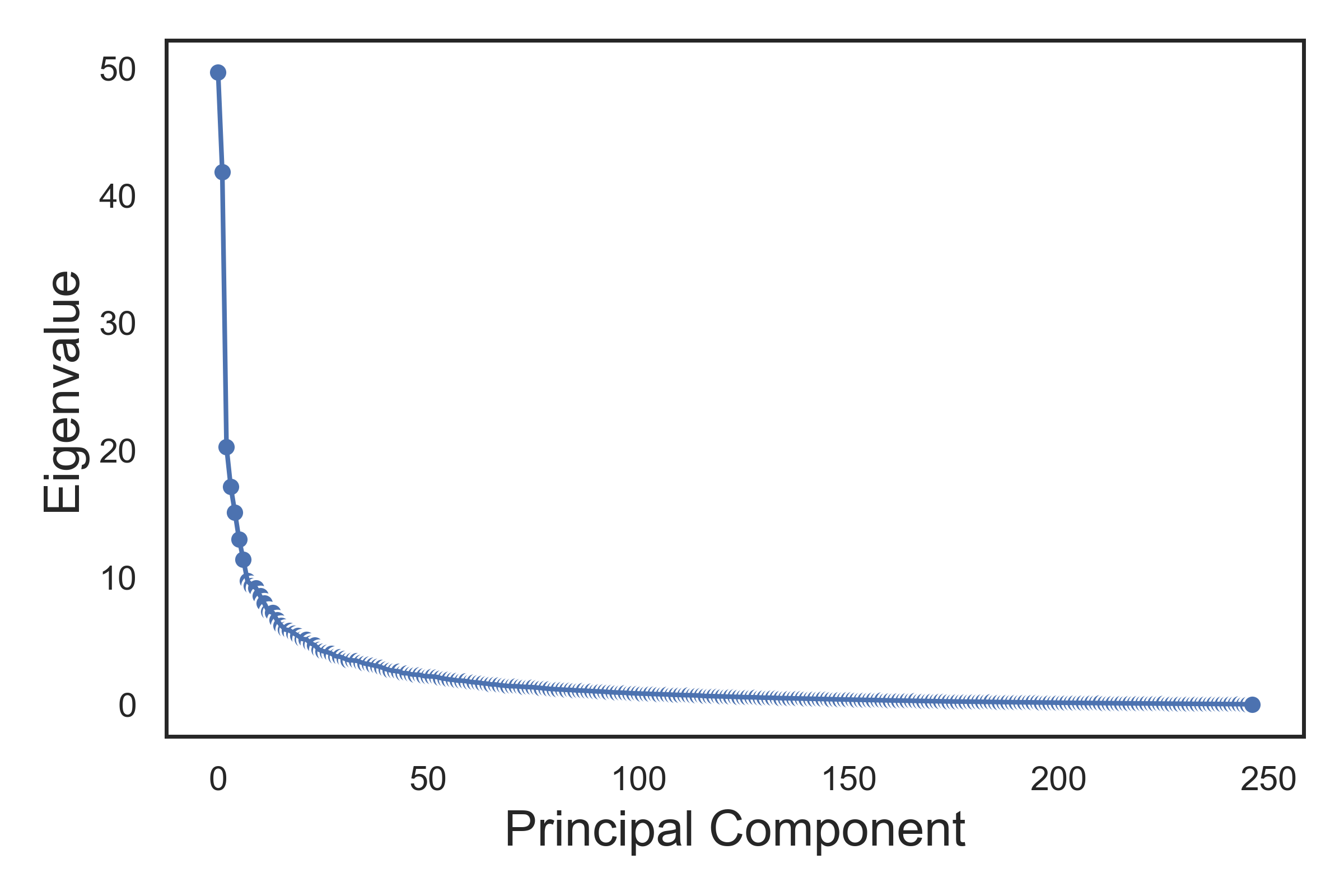
Algorithm 1 summarizes our approach for estimating the matrix of sufficient statistics $\mathbb{S}$. In practice, we might not know what value of $J$ to use in Algorithm 1. To this end, we can use the estimator provided in Section 2.4 of Fan et al. (2013) to estimate $J$. As we show in Section 5, it is often easier to instead visually inspect the spectrum of the sample covariance matrix (referred to as the “scree plot”) to pick $J$.

In the next section, we propose a new score function and prove that it can recover a correct ordering of $\mathcal{G}^{*}$ in 3. We discuss the extension of our consistency result to the $M=\infty$ setting in Appendix C.

3.3 The DeCAMFounder Score Function

We conclude by combining our results so far to derive an estimator for $\mathcal{G}^{*}$. We prove that our approach can recover a correct partial ordering of $\mathcal{G}^{*}$ in the high-dimensional setting when $p,N\rightarrow\infty$. To prove this result, we extend the main theorem in Bühlmann et al. (2014) to the setting when there are pervasive confounders.

Derivation of the DeCAMFounder Score Function. We propose to estimate $\mathcal{G}^{*}$ via a score-based approach. In general, score-based approaches consist of two parts: (1) a score-function to measure the quality of a DAG based on the observed data $\mathbb{X}$, and (2) a combinatorial optimization procedure to optimize this score-function over the space of DAGs. Since there are many existing general-purpose procedures for (2), such as greedy equivalence search, we focus our attention on (1).

A natural starting point (based on its popularity in the linear setting) might be to use the Bayesian information criterion (BIC) as the score function, which penalizes DAGs based on the number of parameters (Chickering, 2002). For linear models, computing this penalty is straightforward because the number of parameters simply equals the number of edges in the graph (corresponding to the number of edge weights to be estimated) and $p$ (the number of node noise variances to be estimated). For semi-parametric models, however, the number of parameters can be infinite. Hence, BIC cannot directly be applied. Instead, we use a Bayesian score, namely the marginal log-likelihood of the DAG (which the BIC approximates with a second-order Taylor series) conditional on the matrix of confounder sufficient statistics $\mathbb{S}$. Specifically, let $\mathbb{Q}(\Omega_{\mathcal{G}}\mid\mathcal{G})$ be a prior over the unknown set of functions $\Omega_{\mathcal{G}}\coloneqq\{\{f_{ij}^{\mathcal{G}}\}_{i\in\textnormal{Pa}_{\mathcal{G}}^{j}},r_{j}^{\mathcal{G}}\}_{j=1}^{p}$ that define the model from 1. Assume that $\mathbb{Q}(\Omega_{\mathcal{G}}\mid\mathcal{G})=\prod_{j=1}^{p}\mathbb{Q}(\{f_{ij}^{\mathcal{G}}\}_{i\in\textnormal{Pa}_{\mathcal{G}}^{j}},r_{j}^{\mathcal{G}}\mid\mathcal{G})$, also known as parameter modularity (Friedman and Nachman, 2000). Given this prior, we score a DAG $\mathcal{G}$ by computing

$$\begin{split}\max_{\sigma^{2}\in\mathbb{R}^{p}_{+}}\log\mathbb{Q}(\mathbb{X}\mid\mathcal{G},\mathbb{S},\sigma^{2})&=\max_{\sigma^{2}\in\mathbb{R}^{p}_{+}}\log\int_{\Omega_{\mathcal{G}}}\mathbb{Q}(\mathbb{X}\mid\mathcal{G},\mathbb{S},\Omega_{\mathcal{G}},\sigma^{2})d\mathbb{Q}(\Omega_{\mathcal{G}}\mid\mathcal{G})\\ &=\sum_{j=1}^{p}\max_{\sigma^{2}_{j}\in\mathbb{R}_{+}}\log\int_{\Omega_{\mathcal{G}}}\mathbb{Q}(\mathbb{X}_{:,j}\mid\mathcal{G},\mathbb{S},\Omega_{\mathcal{G}},\sigma_{j}^{2})d\mathbb{Q}(\Omega_{\mathcal{G}}\mid\mathcal{G})\end{split}$$ (6)

where $\mathbb{X}_{:,j}\in\mathbb{R}^{N}$ denotes the $j$th column of matrix $\mathbb{X}$ and $\sigma^{2}$ denotes a $p$-dimensional vector of unknown noise variances. In the following, we consider the special setting where the priors over the unknown functions in $\Omega_{\mathcal{G}}$ are given by Gaussian processes. This choice on prior allows us to model non-linear relationships, penalize for model complexity, and compute Eq. 6 analytically.

Proposition 1.

Let $\mathcal{G}$ denote a DAG, and $\pi$ a topological ordering of $\mathcal{G}$. Let $GP(0,k)$ denote a zero-mean Gaussian process with positive definite kernel function $k(\cdot,\cdot)$. Assume the following priors on the unknown functions in $\Omega_{\mathcal{G}}$:

$$\begin{split}\ f_{ij}^{\mathcal{G}}(x_{i})&\sim GP(0,k_{ij})\quad\forall\leavevmode\nobreak\ i\in\textnormal{Pa}_{\mathcal{G}}^{j},1\leq j\leq p,\\ r_{j}^{\mathcal{G}}(s_{\pi_{1}},\cdots,s_{\pi_{j-1}})&\sim GP(0,k_{j})\quad\forall\leavevmode\nobreak\ 1\leq j\leq p,\end{split}$$

where $k_{ij}(\cdot,\cdot)$ and $k_{j}(\cdot,\cdot)$ are positive definite kernel functions from $\mathbb{R}\times\mathbb{R}\mapsto\mathbb{R}$ and $\mathbb{R}^{j-1}\times\mathbb{R}^{j-1}\mapsto\mathbb{R}$, respectively. Then, $\log\int_{\Omega_{\mathcal{G}}}\mathbb{Q}(\mathbb{X}_{:,j}\mid\mathcal{G},\mathbb{S},\Omega_{\mathcal{G}},\sigma_{j}^{2})d\mathbb{Q}(\Omega_{\mathcal{G}}\mid\mathcal{G})$ equals

$$-\frac{1}{2}\left(\tilde{\mathbb{X}}_{:,j}^{T}L_{j}^{-1}\tilde{\mathbb{X}}_{:,j}-\log\det L_{j}-N\log(2\pi)\right),\quad\tilde{\mathbb{X}}_{:,j}\coloneqq\mathbb{X}_{:,j}-\mathbb{S}_{:,j},$$ (7)

where $L_{j}=K_{j}+\sigma_{j}^{2}I_{N}$, and the $(n,m)$th entry of the $N\times N$ kernel matrix $K_{j}$ equals

$$\sum_{i\in\textnormal{Pa}_{\mathcal{G}}^{j}}k_{ij}\left(\tilde{x}_{i}^{(n)},\tilde{x}_{i}^{(m)}\right)+k_{j}\left(\left(s_{\pi_{1}}^{(n)},\cdots,s_{\pi_{j-1}}^{(n)}\right),\left(s_{\pi_{1}}^{(m)},\cdots,s_{\pi_{j-1}}^{(m)}\right)\right),\ 1\leq n,m\leq N.$$

We prove 1 in Appendix B. Below we bound the computational complexity of computing Eq. 6.

Corollary 2.

Under the assumptions in 1, $\mathbb{Q}(\mathbb{X}\mid\mathcal{G},\mathbb{S},\sigma^{2})$ takes $O(p^{2}N^{2}+pN^{3})$ time to compute.

Proof.

It suffices to show that $\int_{\Omega_{\mathcal{G}}}\mathbb{Q}(\mathbb{X}_{:,j}\mid\mathcal{G},\mathbb{S},\Omega_{\mathcal{G}},\sigma_{j}^{2})d\mathbb{Q}(\Omega_{\mathcal{G}}\mid\mathcal{G})$ takes $O(pN^{2}+N^{3})$ time to compute by 1. $k_{ij}$ and $k_{j}$ take $O(1)$ and $O(p)$ time to evaluate on a pair of datapoints, respectively. Hence, the $N\times N$ kernel matrix $K_{j}$ takes at most $O(pN^{2})$ time to compute. Computing the determinant and inverse of $L_{j}$ takes $O(N^{3})$ time. Finally, the matrix vector multiplication $\tilde{\mathbb{X}}_{:,j}^{T}L_{j}^{-1}\tilde{\mathbb{X}}_{:,j}$ takes $O(N^{2})$ time. ∎

Algorithm 1 Principal Confounding Sufficient Statistics

1:procedure pcss($\mathbb{X},J$)

2:     $\hat{\Sigma}=\frac{1}{N}\mathbb{X}^{T}\mathbb{X}$

3:     $V,\Lambda,V^{T}=\text{eigen}(\hat{\Sigma})$ $\triangleright$ Eigendecomposition of $\hat{\Sigma}$

4:     $\mathbb{S}=(V_{J}V_{J}^{T}\mathbb{X}^{T})^{T}\in\mathbb{R}^{N\times p}$ $\triangleright$ Sufficient statistics derived in Eq. 5

5:     return $\mathbb{S}$

6:end procedure

Algorithm 2 The DeCAMFounder Score

1:procedure decam($\mathbb{X},\mathcal{G},J$) $\triangleright$ $\mathcal{G}$ a DAG with vertex set $[p]$

2:     $\mathbb{S}=\text{PCSS}(\mathbb{X},J)$ $\triangleright$ Computed from Algorithm 1

3:     $\pi$ is a topological order of $\mathcal{G}$

4:     $mll=0$

5:     for $1\leq j\leq p$ do

6:         $mll=mll+\max_{\sigma_{j}^{2}}$[ Eq. 7 ] $\triangleright$ Maximize via gradient ascent

7:     end for

8:     return $mll$$\triangleright$ The log marginal likelihood of $G$.

9:end procedure

We summarize our final derived score function in Algorithm 2. In our implementation of the DeCAMFounder score, we use GPyTorch (Gardner et al., 2018) to fit the noise variances and kernels via gradient ascent. In Appendix D, we detail the particular kernel functions used in our experiments. We now turn our attention to proving when maximizing the DeCAMFounder score recovers a consistent ordering of $\mathcal{G}^{*}$.

Theoretical Guarantees. Assume that $\mathcal{G}^{*}\in\mathfrak{G}$ for some set of DAGs $\mathfrak{G}$ with vertices $\{X_{j}\}_{j=1}^{p}$. Let $\Pi_{*}\subset\mathfrak{G}$ consist of all DAGs with partial orderings consistent with that of $\mathcal{G}^{*}$, namely $\Pi^{*}=\{\mathcal{G}\in\mathfrak{G}:i\in\textnormal{An}_{\mathcal{G}^{*}}^{j}\implies i\in\textnormal{An}_{\mathcal{G}}^{j}\}$, where $\textnormal{An}_{\mathcal{G}}^{j}$ denotes the set of ancestors of $X_{j}$ in $\mathcal{G}$. To prove that an estimator recovers a true ordering of $\mathcal{G}^{*}$, it suffices to show that it selects a DAG in $\Pi_{*}$ with probability tending towards 1 as $N\rightarrow\infty$. In Bühlmann et al. (2014), the authors proved consistency of the MLE for causal additive models. 3 extends the main result in Bühlmann et al. (2014) to the more general setting when there are pervasive confounders. To prove this result we need to make a number of different assumptions, which we now discuss further.

Assumption 4.

For all $1\leq j\leq p$, there exists some function $q_{j}$ such that ${\color[rgb]{0,0,0}\definecolor[named]{pgfstrokecolor}{rgb}{0,0,0}\pgfsys@color@gray@stroke{0}\pgfsys@color@gray@fill{0}r_{j}(S_{1},\ldots,S_{j-1})}=q_{j}(S_{\textnormal{Pa}_{\mathcal{G}^{*}}^{j}})$ in 1, where $S_{\textnormal{Pa}_{\mathcal{G}^{*}}^{j}}$ restricts the components of $S$ to the set of indices that belong to the parent set of $X_{j}$ in $\mathcal{G}^{*}$.

In general, $r_{j}(S_{1},\ldots,S_{j-1})$ depends on $j-1$ variables, which makes estimation challenging when $j$ is large. 4 ensures that each $r_{j}$ depends on a sparse number of components in $S$ whenever the true DAG $\mathcal{G}^{*}$ is sparse, making estimation significantly easier. When $f_{ij}$ is a linear function, then 4 always holds, see Eq. 14. With slight abuse of notation, in the remainder of this section we use $r_{j}(S_{\textnormal{Pa}_{\mathcal{G}}^{j}})$ to denote $q_{j}(S_{\textnormal{Pa}_{\mathcal{G}}^{j}})$.

The next assumption concerns sufficient “model separation”, measured in terms of the negative log-likelihood scores of different DAGs. By 1, Gaussianity of the errors, and 4, the expected negative log-likelihood score of a DAG $\mathcal{G}$ equals $\sum_{j=1}^{p}\log(\sigma_{j}^{\mathcal{G}})+p\sqrt{2\pi}+.5p$ (Bühlmann et al., 2014), where

$$\begin{split}&\left(\sigma_{j}^{\mathcal{G}}\right)^{2}\coloneqq\mathbb{E}_{\mathbb{Q}}\left[\left(X_{j}-\sum_{i\in\textnormal{Pa}_{\mathcal{G}}^{j}}f_{ij}^{\mathcal{G}}(X_{i})-S_{j}+r_{j}^{\mathcal{G}}(S_{\textnormal{Pa}_{\mathcal{G}}^{j}})\right)^{2}\right]\\ \left\{f_{ij}^{\mathcal{G}}\right\}_{i\in\textnormal{Pa}_{\mathcal{G}}^{j}},r_{j}^{\mathcal{G}}=&\operatorname*{arg\,min}_{g_{ij}\in\tilde{\mathcal{F}}_{ij},\ w_{j}\in\tilde{\mathcal{R}}_{j}^{\mathcal{G}}}\mathbb{E}_{\mathbb{Q}}\left[\left(X_{j}-\sum_{i\in\textnormal{Pa}_{\mathcal{G}}^{j}}g_{ij}(X_{i})-S_{j}-w_{j}(S_{\textnormal{Pa}_{\mathcal{G}}^{j}})\right)^{2}\right]\end{split}$$ (8)

and $\tilde{\mathcal{F}}_{ij}$ and $\tilde{\mathcal{R}}_{j}^{\mathcal{G}}$ denote the reproducing kernel Hilbert spaces induced by the kernels $k_{ij}$ and $k_{j}$ in 1 for $1\leq j\leq p$, respectively. We define the model-separation parameter $\xi_{p}$ as the difference in the normalized negative log-likelihood score of the best incorrect DAG and correct DAG:

$$\xi_{p}=p^{-1}\min_{\mathcal{G}\notin\Pi_{*}}\sum_{j=1}^{p}\left(\log\left(\sigma_{j}^{\mathcal{G}}\right)-\log\left(\sigma_{j}^{\mathcal{G}^{*}}\right)\right).$$

If $\mathcal{G}\not\in\Pi_{*}$, $\tilde{\mathcal{F}}_{ij}$ and $\tilde{\mathcal{R}}_{j}^{\mathcal{G}^{*}}$ contain the true unknown functions generating the SCM in 1 for $1\leq j\leq p$, and the requirements in 1 are satisfied, then $\xi_{p}>0$. This non-zero gap occurs because the function class is restricted to additive functions of the observed variables; regression on the wrong order induces a different density than $\mathbb{Q}(X\mid S)$. Hence, the KL divergence is negative which implies $\xi_{p}>0$. Consequently, the partial ordering is identifiable.

To prove 3, we require that $\xi_{p}$ is large enough to offset the estimation error of having a finite number of datapoints, and noisy estimates of $\{s^{(n)}\}_{n=1}^{N}$.

Assumption 5.

(model-separation gap) $\xi_{p}>0$, and for the constant $c$ in 2,

$$\left(\log(N)^{1/c}\sqrt{\frac{\log p}{N}}+\frac{N^{\frac{1}{4}}}{\sqrt{p}}\right)=o(\xi_{p})$$

In Bühlmann et al. (2014), the authors require that $\xi_{p}$ grows faster than $\sqrt{\frac{\log p}{N}}$ as $p,N\rightarrow\infty$. We require a stronger gap due to the additional error from estimating $\{s^{(n)}\}_{n=1}^{N}$. When $p=\Omega(N^{3/2})$, the model-separation gap requirement is $O\left(\log(N)^{1/c}\sqrt{\frac{\log p}{N}}\right)$, and only differs from the requirement in Bühlmann et al. (2014) by a log factor.

The remaining assumptions used to prove 3 closely resemble those in Bühlmann et al. (2014), where we make minor modifications to handle the $r_{j}$ component in 1. As in Bühlmann et al. (2014), we assume that $\mathcal{G}^{*}$ is sparse, and that the function classes $\tilde{\mathcal{F}}_{ij}$ and $\tilde{\mathcal{R}}_{j}^{\mathcal{G}}$ are finite-dimensional with bounded log-bracketing numbers; see 8 through 10 in Section B.6. Our proof of 3, which shows that the DeCAMFounder asymptotically recovers the true partial ordering of $\mathcal{G}^{*}$, is provided in Section B.6.

Theorem 3.

Let $\widehat{\mathcal{G}}$ be the DAG that maximizes the score in Algorithm 2 over $\mathfrak{G}$. Suppose that the assumptions in 2 hold, and additionally that 4, and 8 through 10 in Section B.6 hold. If $N=o(p^{2})$ and $p=o(\exp(N))$, then

$$\mathbb{P}(\widehat{\mathcal{G}}\in\Pi_{*})\rightarrow 1\quad\text{as}\quad p,N\rightarrow\infty.$$

The rate constraint in 3 is satisfied, for example, when $p=\Theta(N)$. In Appendix C, we extend 3 to handle the case when 1 does not hold by using a similar idea in Bühlmann et al. (2014) to handle model misspecification.

4 Related Work

Two main approaches have been proposed for learning causal structures in the presence of confounders. The first approach focuses on modeling the conditional independence structure of $\mathbb{Q}(X)$ using an ancestral graph and subsequently recovering the edges in this graph. Examples of algorithms for ancestral graph estimation include FCI (Spirtes et al., 2000), RFCI (Colombo et al., 2012), and GSPo (Bernstein et al., 2020). However, these methods recover fewer causal relationships since they make minimal assumptions about the confounders, as illustrated in Figure 1 of Frot et al. (2019).

The second approach makes more assumptions about the confounders, and tries to exploit these structural assumptions for better estimation. One commonly used assumption is that the confounders are sources in the graph (“exogenous”) and have an effect on many observed variables (“pervasive”). For linear Gaussian graphical models with exogenous pervasive confounders, several methods have been proposed to accurately estimate the covariance matrix of the conditional distribution $\mathbb{Q}(X\mid H)$ using only data points drawn from $\mathbb{Q}(X)$ for the purposes of conditional independence testing (Chandrasekaran et al., 2012; Fan et al., 2013; Frot et al., 2019; Shah et al., 2020). The methods for estimating the covariance matrix associated with $\mathbb{Q}(X\mid H)$, which in the linear Gaussian case is the same for all $H$, fall into two classes: the optimization approach and the spectral approach.

Optimization Approach: Deconfounding the Precision Matrix. Frot et al. (2019) decompose the precision matrix of $(X,H)$ into the blocks

$$[\text{Cov}((X,H))]^{-1}=\begin{pmatrix}\begin{matrix}J_{O}\end{matrix}&\vline&J_{OH}\\ \hline\cr J_{HO}&\vline&\begin{matrix}J_{H}\end{matrix}\end{pmatrix}.$$

By standard theory for multivariate Gaussian distributions, $J_{O}\in\mathbb{R}^{p\times p}$ is the precision matrix associated with the conditional distribution $\mathbb{Q}(X\mid H)$. The key idea for estimating $J_{O}$ is to relate the observed precision matrix $[\text{Cov}(X)]^{-1}$ and the target quantity $J_{O}$ via Schur complements:

$$[\text{Cov}(X)]^{-1}=J_{O}-J_{OH}J_{HH}^{-1}J_{HO}.$$

For sparse DAGs, $J_{O}$ is a sparse matrix, and when $K\ll p$, $J_{OH}J_{HH}^{-1}J_{HO}$ is low-rank. Hence, when the confounders are pervasive, it is possible to estimate each component through a low-rank plus sparse matrix decomposition of $[\text{Cov}(X)]^{-1}$ (Frot et al., 2019; Chandrasekaran et al., 2009, 2012).

Spectral Approach: Deconfounding the Covariance Matrix. In contrast to the optimization approach, Shah et al. (2020) directly estimates the covariance matrix. Under the SCM in Eq. 2,

$$\begin{split}\text{Cov}(X)&=(I-B)^{-1}\Lambda(I-B)^{-T}+(I-B)^{-1}\Theta\Theta^{T}(I-B)^{-T}\\ &=(I-B)^{-1}\Lambda(I-B)^{-T}+\tilde{\Theta}\tilde{\Theta}^{T}\quad\text{s.t.}\quad\tilde{\Theta}=(I-B)^{-1}\Theta\\ &=\underbrace{J_{O}^{-1}}_{\text{sparse inverse}}+\underbrace{\tilde{\Theta}\tilde{\Theta}^{T}}_{\text{low-rank}}.\end{split}$$ (9)

If the confounders are pervasive, then the eigenvalues of $\tilde{\Theta}\tilde{\Theta}^{T}$ grow linearly with the dimension $p$, while the eigenvalues of $J_{O}^{-1}$ are assumed to grow much slower. As a result, the spectrum of $\text{Cov}(X)$ is dominated by the spectrum of $\tilde{\Theta}\tilde{\Theta}^{T}$. Hence, the top principal components of $\text{Cov}(X)$ approximate $\tilde{\Theta}\tilde{\Theta}^{T}$ well, and consequently provide a way to estimate $J_{O}^{-1}$ (Fan et al., 2013; Wang and Fan, 2017). In settings when the gap between the eigenvalues of $J_{O}^{-1}$ and $\tilde{\Theta}\tilde{\Theta}^{T}$ in Eq. 9 is small, Shah et al. (2020) propose a modified covariance estimator. Outside of the graphical models literature, such spectral approaches are similar to the approach proposed by Wang and Blei (2019) to estimate average treatment effects in the potential outcomes framework.

5 Experiments

We begin our empirical evaluation by examining the performance of the Principal Confounding Sufficient Statistics (PCSS) procedure, outlined in Algorithm 1, in estimating the confounder sufficient statistics $S=\mathbb{E}[X\mid H]$. This analysis is presented in Section 5.1.1. We investigate the impact of estimation errors in PCSS on the performance of our DeCAMFounder score function, which is discussed in Section 5.1.2 and Section 5.2.2. To provide a comprehensive comparison, we benchmark our DeCAMFounder score function against other commonly used score functions in the fully-observed or pervasive confounding settings. Detailed descriptions of these benchmark methods are provided in Section 5.1.2.

To establish a known ground truth DAG, we conduct our evaluation using simulated data. This allows us to assess the accuracy of our method. In addition to the simulated data, we evaluate our approach on a real ovarian cancer dataset in Section 5.2. The use of this dataset enables partial validation based on prior biological knowledge of the underlying system. We express our gratitude to the authors of Frot et al. (2019) for providing a pre-processed and easily reproducible version of this dataset. All the results presented in this section can be reproduced using the provided data and code, which are accessible at https://github.com/uhlerlab/decamfound.

5.1 Simulated Data

In this set of simulations, we examine the robustness of our method to different data characteristics. To achieve this, we vary the following parameters: the strength of confounding, linear or non-linear SCM, and dimensionality.

Controlling the Strength of Confounding. Generating non-linear (and even linear) data can be challenging. For example, without proper normalization, the variance of downstream nodes can explode (e.g., consider a line graph $X_{1}\rightarrow X_{2}\cdots\rightarrow X_{p}$ with edge weights larger than 1). Additionally, if the noise variance is the same across nodes, downstream nodes typically exhibit a higher signal-to-noise ratio than upstream nodes. To mitigate any biases introduced by such artifacts in the data simulation process, we apply the following normalization (note that specific edge cases arise for source nodes or those independent of $H$; refer to Appendix E for further details):

• Unit variance nodes: $\text{Var}(X_{j})=1$ for all $1\leq j\leq p$.

• Zero mean nodes: $\mathbb{E}[X_{j}]=0$ for all $1\leq j\leq p$.

• Fixed signal, confounding, and noise variances: for all $1\leq j\leq p$:

  • $\text{Cov}(X_{j},\epsilon_{j})=\sigma^{2}_{\text{noise}}$,

  • $\text{Cov}(\sum_{k=1}^{K}g_{kj}(H_{k}))=\sigma_{h}^{2}$, and

  • $\text{Cov}(\sum_{i\in\textnormal{Pa}_{\mathcal{G}^{*}}^{j}}f_{ij}(X_{i}))=\sigma^{2}_{\text{signal}}$.

Since all nodes have unit variance, $\sigma_{h}^{2}$ equals the fraction of the variation in $X_{j}$ explained by $H$, and $\sigma_{\text{signal}}^{2}$ equals the fraction of the variation in $X_{j}$ explained by its parents. In our experiments, we fix $\sigma^{2}_{\text{noise}}=0.2$. In other words, if we could actually observe both $X$ and $H$, then the noise in the problem is small. To assess how the strength of confounding affects DAG recovery, we vary $\sigma_{h}^{2}$. Note that $\sigma_{\text{signal}}^{2}$ is a deterministic function of $\sigma_{h}^{2}$: $\sigma_{\text{signal}}^{2}=\text{Var}(X_{j})-\sigma_{\text{noise}}^{2}-\sigma_{h}^{2}=0.8-\sigma_{h}^{2}$. Therefore, varying $\sigma_{h}^{2}$ implicitly varies the observed signal variance $\sigma^{2}_{\text{signal}}$.

Linear / Non-Linear SCM. We randomly draw each $f_{ij}$ and $g_{kj}$ in Eq. 1 from the set of linear trends $\{\theta x:\theta\in\mathbb{R}\}$, seasonal trends $\{\theta\sin(\pi x):\theta\in\mathbb{R}\}$, or quadratic trends $\{\theta x^{2}:\theta\in\mathbb{R}\}$ when generating non-linear data. For data generated from a linear SCM, we assume that each $f_{ij}$ and $g_{kj}$ belongs strictly to the set of linear trends.

Data Generation. We randomly draw $\mathcal{G}^{*}$ from an Erdös-Rényi random graph model with expected neighborhood size of $5$ and consider graphs with number of observed nodes $p\in\{250,500,1000\}$. As in Frot et al. (2019), we assume that each confounder is a direct cause of an observed variables with a $70\%$ chance. Given the graph, we randomly select a trend type for each edge (i.e., the $f_{ij}$ and $g_{kj}$ in Eq. 1) with equal probability. We then randomly draw a weight $\theta\sim\text{Uniform}([-1,-.25]\cup[.25,1])$ and appropriately scale weights of all parents simultaneously to satisfy the normalization constraints above. We finally add $N(0,\sigma_{\text{noise}}^{2})$ noise to each node; see Appendix E for more details and references to our python code. Unless otherwise stated, we draw 25 random datasets for each specific configuration of confounding strength and dimensionality. We consider $K=1$ pervasive confounders, which allows us to plot how each node varies as a function of this confounder. See Appendix F for our empirical results for other choices of $K$.

5.1.1 Confounder Sufficient Statistics Estimation Performance

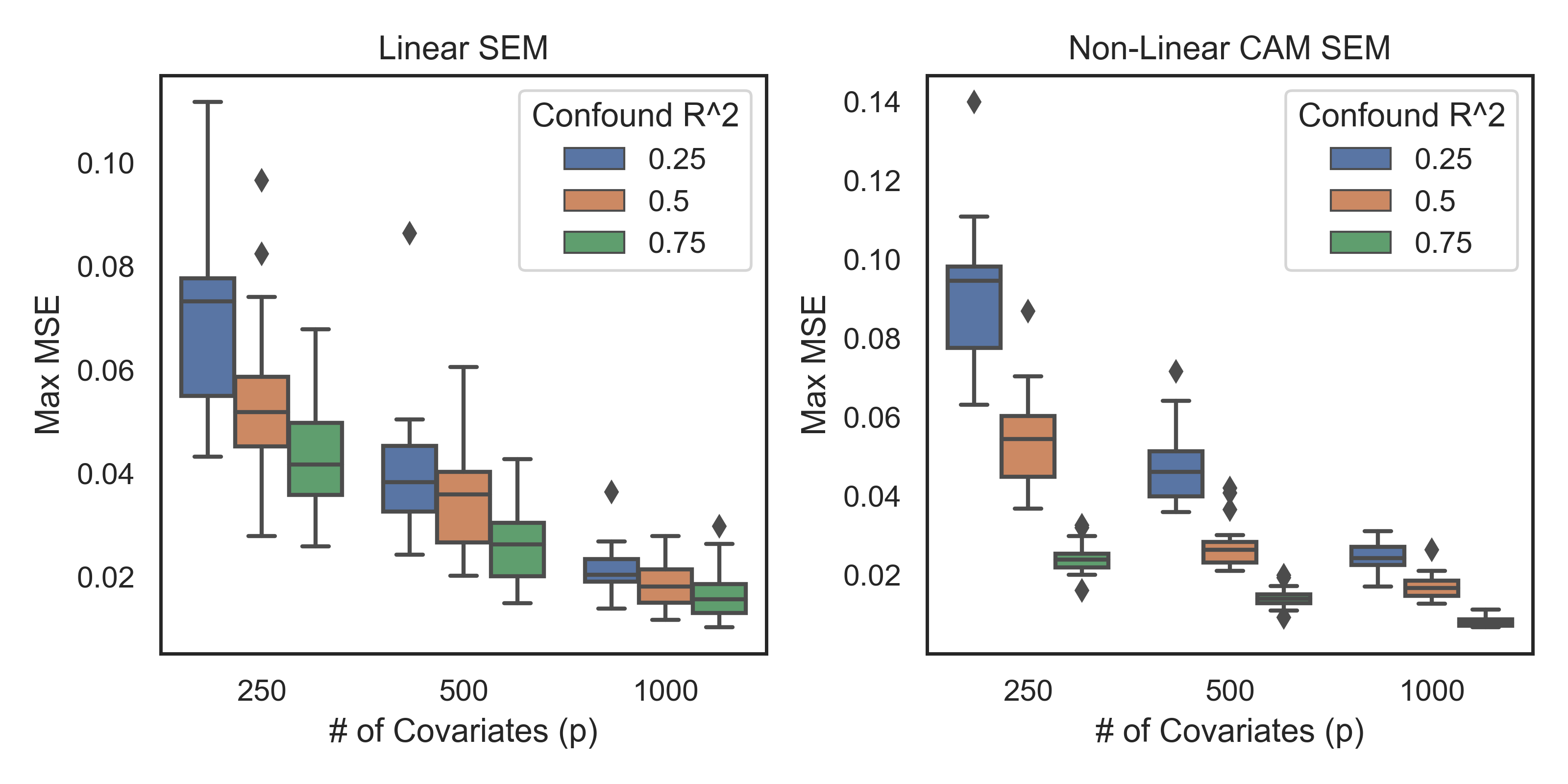
Based on 2, our estimate of the confounder sufficient statistics should decrease as $N$ and $p$ increase. To test this empirically, we keep the ratio of $\frac{p}{N}$ fixed at 2, and vary the confounding strength and dimensionality. Fig. 2 plots the maximum mean-squared error, which equals $\max_{1\leq j\leq p}\frac{1}{N}\sum_{n=1}^{N}\left(s_{j}^{(n)}-\hat{s}_{j}^{(n)}\right)^{2}$. In the linear case, we can compute $S$ analytically as a function of $H$ (see 1). However, in the non-linear case, there is no analytical expression for $S$ in term of $H$. Nonetheless, if $X_{j}$ only has confounders as parents, then $S_{j}=\sum_{k=1}^{K}g_{kj}(H_{k})$. Thus, in Fig. 2, the max MSEs for the non-linear SCM case are only with respect to the $S_{j}$ associated with nodes that only have confounders as parents. From Fig. 2, we see that the MSE decreases as $p$ increases or when the strength of the confounders increases.

Figure 2: Maximum Mean-Squared Error (MSE) across all dimensions for estimating $\{s^{(n)}\}_{n=1}^{N}$ via PCSS. Twenty-five total simulations were performed for each dataset configuration.

To evaluate the quality of PCSS for nodes that also have observed nodes as parents, we can make qualitative assessments. In particular, since there are only $K=1$ confounders, we can plot $x_{j}^{(n)}$ against $h_{1}^{(n)}$. The visual trend we see from the resulting scatterplot corresponds to the desired conditional expectation $s_{j}^{(n)}=\mathbb{E}[X_{j}\mid H_{1}=h_{1}^{(n)}]$. By plotting the confounder sufficient statistics estimated from PCSS on the same plot for each dimension, we can qualitatively check for a matching trend. Fig. 3 provides such a plot for a particular random data simulation and select nodes that have at least one parent. We see that PCSS indeed matches the data trend well.

Figure 3: Non-linear estimation of $E[X_{i}\mid H]$ via PCSS for nodes with at least one parent.

5.1.2 Evaluation of the DeCAMFounder Score

We now evaluate how well the DeCAMFounder scores DAGs using noisy estimates of the confounder sufficient statistics. For this evaluation, we separate the merits of the score function from the selected optimization procedure. In particular, since many optimization procedures for DAG estimation greedily optimize over parent sets, we focus on the task of effectively scoring parent sets.

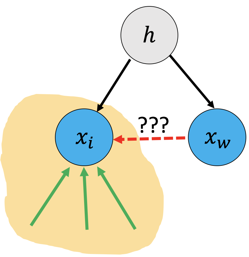
Description of the Parent Set Evaluation Tasks. In greedy procedures, changes to a parent set typically involve a single node addition (adding a node to the current parent set) or deletion (removing a node from the current parent set). In the presence of latent confounding, methods that do not account for confounders are susceptible to adding spurious edges. For example, suppose nodes $X_{i}$ and $X_{j}$ have a common hidden cause but no shared parents in $\mathcal{G}^{*}$ for some $1\leq i,j\leq p,i\neq j$. Then, a method that assumes no latent confounding might add an edge from $X_{i}$ to $X_{j}$ or vice versa with high probability, even when all the true parents of the node are included in the current parent set.

This observation leads to a natural evaluation procedure: consider the set of all nodes $C\coloneqq\{X_{j}:D_{j}\neq 0,1\leq j\leq p\}$ that have direct confounders (see Eq. 1 for the definition of $D_{j}$). Randomly select a node $X_{j^{\prime}}$ from $C$ and randomly sample $T$ nodes $X_{r_{1}},\ldots,X_{r_{T}}$ from $C$ that are not parents of $X_{j^{\prime}}$. Then, we evaluate the methods in terms of scoring the following $T+1$ parent sets:

$$\begin{split}P_{\text{correct}}&=\textnormal{Pa}_{\mathcal{G}^{*}}^{j^{\prime}}\\ P_{t}&=\textnormal{Pa}_{\mathcal{G}^{*}}^{j^{\prime}}\cup\{X_{r_{t}}\}\quad\text{for}\quad{\color[rgb]{0,0,0}\definecolor[named]{pgfstrokecolor}{rgb}{0,0,0}\pgfsys@color@gray@stroke{0}\pgfsys@color@gray@fill{0}1\leq t\leq T}.\\ \end{split}$$

Again, we might expect that methods that do not correct for confounders score some $P_{t}$ higher than $P_{\text{correct}}$ due to spurious correlations created by the confounders. In our evaluation, we pick $T=100$. We call this evaluation procedure the Wrong Parent Addition Task. We note that this task is similar to the “CauseEffectPairs” causality challenge introduced by Mooij et al. (2016).

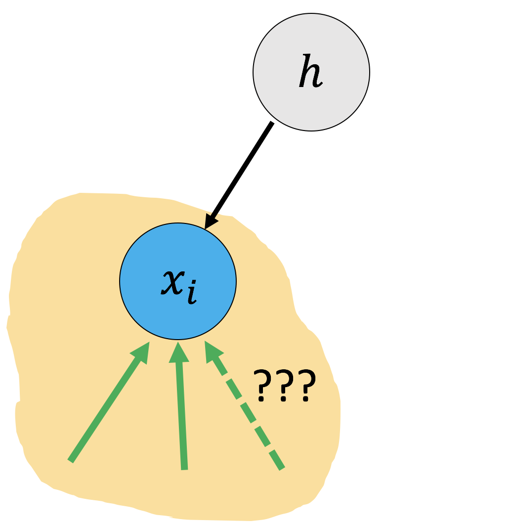
The second parent set evaluation task concerns the node deletion phase. Here, we expect that linear methods may suffer by potentially removing true parent nodes. For example, if a parent node has low correlation with its child (e.g., as is the case with our sine and quadratic trends), then that parent might be removed when using a sparsity-inducing score function such as BIC or penalized log-likelihood with an $L_{0}$ or $L_{1}$ penalty.

Similar to the Wrong Parent Addition task, we first randomly select a node $X_{j^{\prime}}$ with at least one observed parent node, where $1\leq j^{\prime}\leq p$. For each node in the parent set of $X_{j^{\prime}}$, let

$$\begin{split}P_{\text{correct}}&=\textnormal{Pa}_{\mathcal{G}^{*}}^{j^{\prime}}\\ P_{t}&=\textnormal{Pa}_{\mathcal{G}^{*}}^{j^{\prime}}\setminus\{X_{i}\}\quad\text{for}\quad X_{i}\in\textnormal{Pa}_{\mathcal{G}^{*}}^{j^{\prime}}.\\ \end{split}$$

We would again like to understand if certain score functions favor incorrect $P_{t}$ parent sets when the parents have non-linear effects on the target. We call this evaluation procedure the Correct Parent Deletion task. These two tasks are illustrated in Fig. 4.

(a) Wrong Parent Addition

(b) Correct Parent Deletion

Figure 4: Our parent set evaluation tasks. Solid arrows represent the set of true edges, and dotted arrows indicate a potential incorrect modifcation to the true parent set of a node.

Benchmark Methods. We now describe our benchmark scoring methods. The first three methods are linear, and use the BIC score with different estimates of the covariance matrix. In particular, the BIC score (under Gaussian errors) is a function of a target node $X_{j}$, parent set $P_{j}\subset\{1,\cdots,p\}\setminus\{j\}$, and estimated covariance matrix $\hat{\Sigma}\in\mathbb{R}^{p\times p}$, $1\leq j\leq p$:

$$\text{BIC}(X_{j},P_{j},\hat{\Sigma})=-\left(\frac{N}{2}\log\left(2\pi\hat{\sigma}_{j\mid P_{j}}^{2}\right)+\frac{N}{2}\right)-.5\log(N)(|P_{j}|+2),$$ (10)

where the conditional noise variance (based on Schur complements) equals

$$\hat{\sigma}_{j\mid P_{j}}^{2}=\hat{\Sigma}_{jj}-\hat{\Sigma}_{jP_{j}}\hat{\Sigma}_{P_{j}P_{j}}^{-1}\hat{\Sigma}_{P_{j}j}.$$

The benchmarks are as follows:

1. Vanilla-BIC: scores each parent set by inputting the sample covariance matrix $\frac{1}{N}\mathbb{X}^{T}\mathbb{X}$ into Eq. 10.

2. LRPC+BIC: scores each parent using the covariance matrix estimated from a low-rank plus sparse (LRPS) decomposition of the sample precision matrix; see Frot et al. (2019). We use the author’s code in R to fit this decomposition, and pick the hyperparameters using cross-validation.

3. PCSS-BIC: scores each parent using the covariance matrix $\frac{1}{N}(\mathbb{X}-\mathbb{S})^{T}(\mathbb{X}-\mathbb{S})$, where $\mathbb{S}$ is the output from Algorithm 1. We pick one principal component and 3 principal components for the linear and non-linear case, respectively. This choice was based on visual inspection of the spectrum of the covariance matrix. See the Appendix.

4. CAM: scores each parent via Eq. 7 but sets $\mathbb{S}_{:,j}$ equal to the zero matrix. This method corresponds to fitting a standard causal additive model without correcting for the confounders.

5. CAM-OBS: scores each parent by computing Eq. 6 but replacing $\mathbb{S}$ with the actual confounders $\mathbb{H}$. This method corresponds to fitting a standard causal additive model when both $X$ and $H$ are observed, and is therefore not realizable in practice.

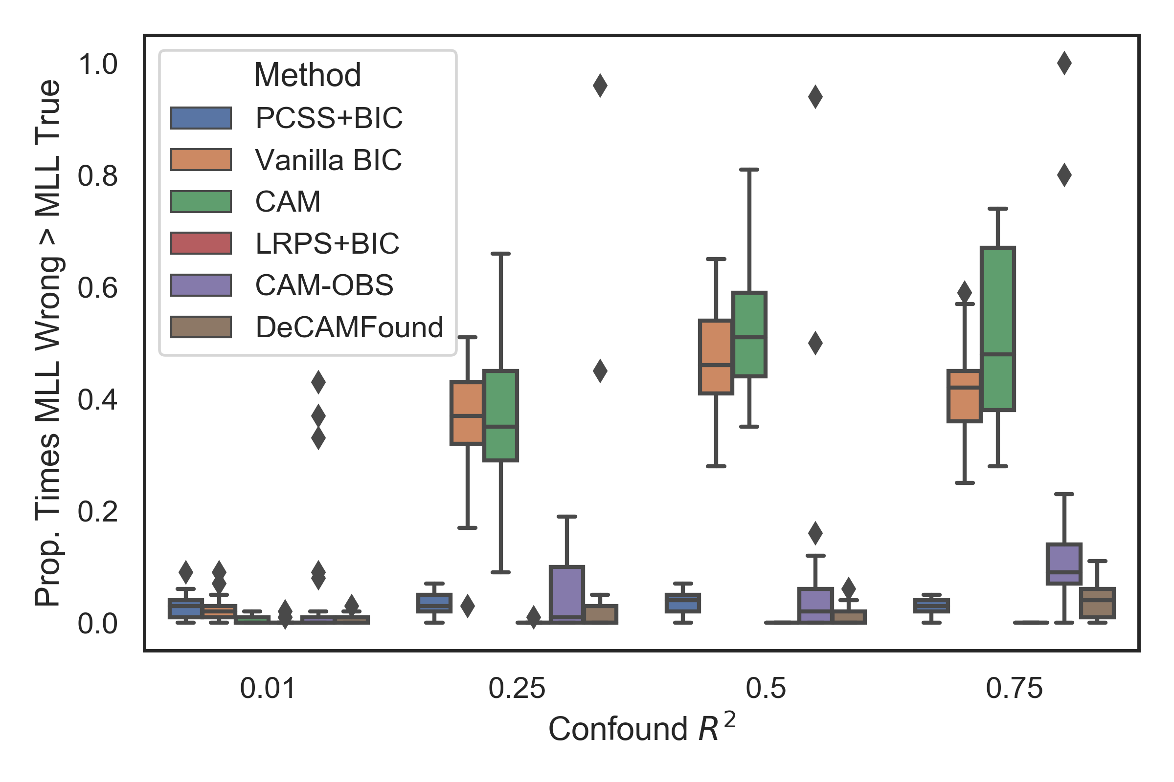
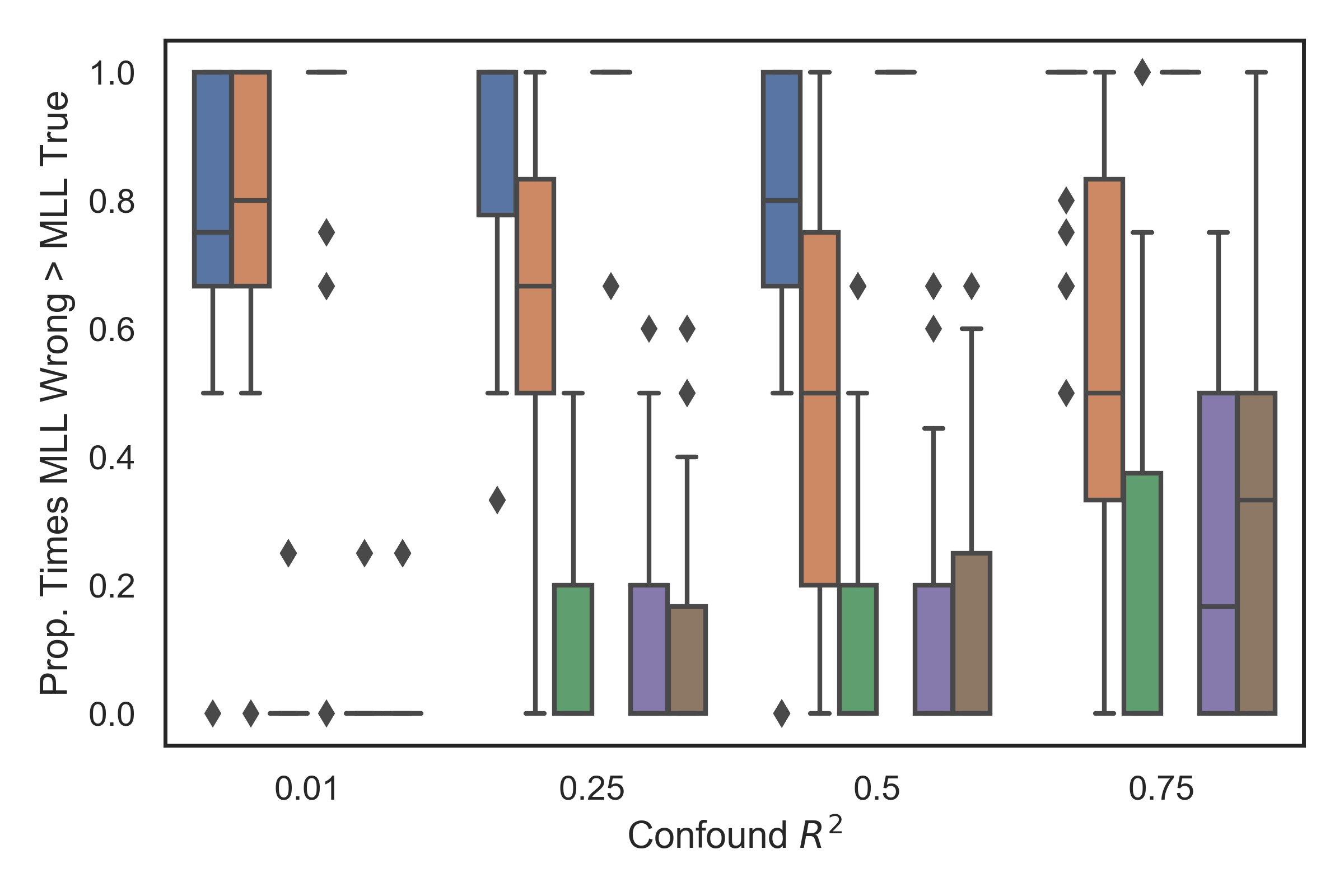
For both parent set tasks, we fix $N=250$ and $p=500$ but vary the strength of confounding. For the Correct Parent Deletion task, we exclude the linear trend from the set of trends when generating non-linear data to focus on the particular problem of modeling non-linearities. Apart from that, the data in both settings are generated as specified at the beginning of this section. Fig. 5 shows the non-linear SEM results. The remaining results are shown in Fig. G.1 and Fig. G.2. In these figures, the different methods are compared using the following metric:

Prop. Times MLL Wrong $>$ MLL True: out of the $T$ incorrect parent sets, what proportion have scores larger than the true parent set. Lower is better here.

Fig. 5 and Fig. G.1 show that methods that account for confounders (i.e., LRPC+BIC, PCSS-BIC, CAM-OBS, DeCAMFound), place higher probability on the correct parent set for the Wrong Parent Addition task across different settings relative to those that do not model the confounders. In addition, Fig. 5 and Fig. G.2 show that for the Correct Parent Deletion task, the linear methods suffer in the non-linear setting. Note that unlike PCSS-BIC, LRPC+BIC suffers even in the linear setting because it induces a very sparse graph, causing it to delete true parents.

Including CAM-OBS in our evaluation allows us to understand how parent set recovery is affected by estimation error from only having a finite amount of observational data. Interestingly, our method, which does not require knowing $H$, sometimes outperforms CAM-OBS. This might be because our method leverages all $p$ observed nodes to estimate the confounding variation via PCA. CAM-OBS, on the other hand, estimates the confounding variation one node at a time by regressing each observed node on $H$. Finally, all methods suffer when the confounding strength increases since the observed signal necessarily becomes weaker. We provide additional empirical results including a DAG evaluation scoring task in Section G.1.

(a) Wrong Parent Addition Task

(b) Correct Parent Deletion Task

Figure 5: Results for the Wrong Parent Addition and Correct Parent Deletion tasks (lower values on the y-axis are better for both tasks). The data are generated according to a non-linear SEM. 25 total simulations per dataset configuration were performed.

5.2 Real Data: Ovarian Cancer Dataset

We use the ovarian cancer RNA-seq dataset from Frot et al. (2019) for our real-data analysis, which consists of $N=247$ human samples and $p=501$ genes. There are 15 total transcription factors (TFs), and the remaining 486 genes interact with at least one of these TFs. This dataset has a partial ground truth; the 15 TFs can only be causes and not effects of the 486 genes. The reference network for the 501 variables is obtained using Netbox, a software tool for performing network analysis using biological knowledge and community network-based approaches (Cerami et al., 2010). A caveat, however, is that edges in this network might not have a precise causal interpretation.

One metric used by Frot et al. (2019) was a count of the number of directed edges from TFs to genes that agree with the edges in NetBox. The authors stated that confounding can be expected in this dataset due to unobserved transcription factors or batch effects. We here take a different approach for the evaluation and instead explicitly create confounders by design. In particular, we remove all 15 TFs from the dataset and assume that we only observed the remaining 486 genes.

Figure 6: The two genes most positively and negatively correlated with the transcription factor NFKB1, respectively. GENE-pcss refers to the total latent confounding variation estimated for that gene via PCSS. GENE refers to the observed values of the gene.

Figure 7: Both genes have a correlation greater than 0.4 with NFKB1 (left hand plot). After subtracting out the confounding variation estimated using PCSS for each gene (denoted as “deconfounded” expression level), the genes are no longer correlated with the unobserved transcription factor NFKB1.

5.2.1 Estimating the Confounding Variation

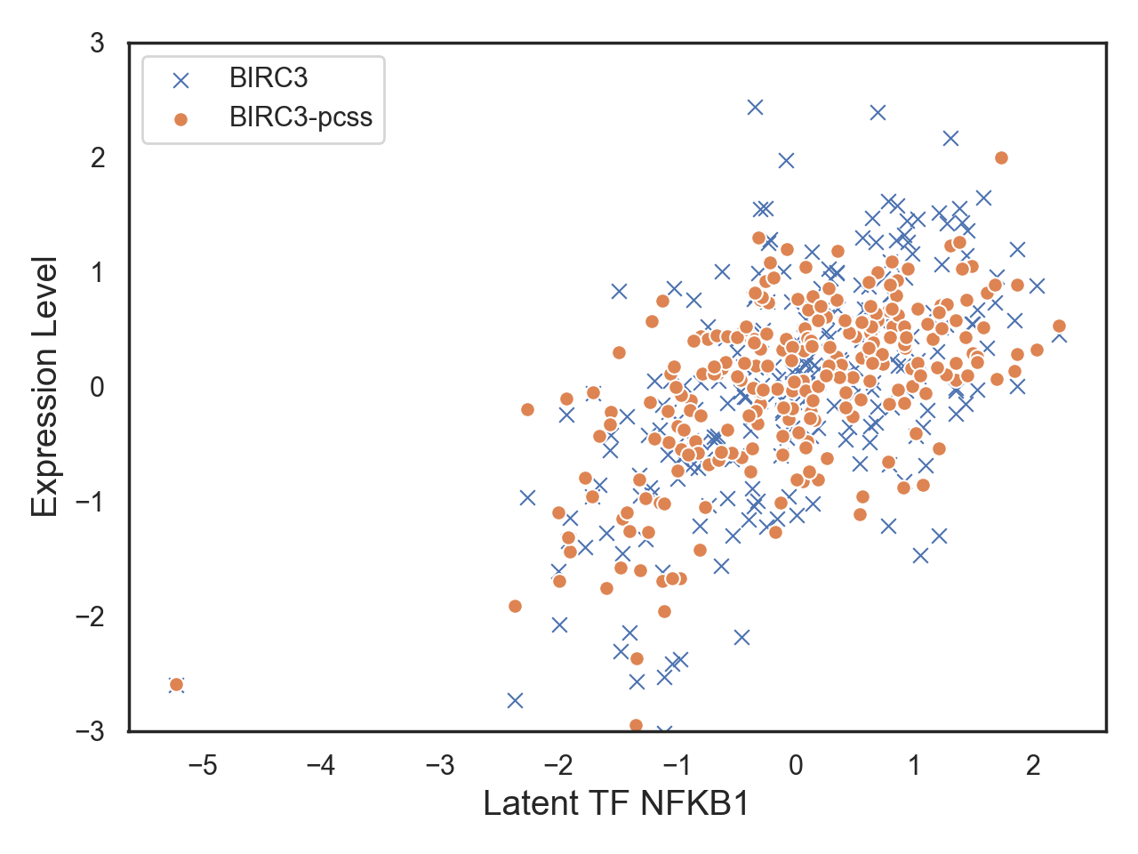
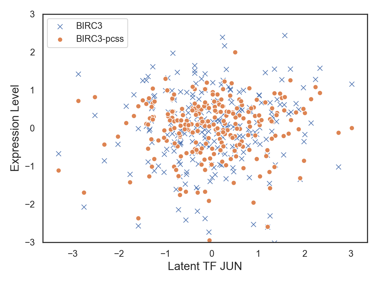
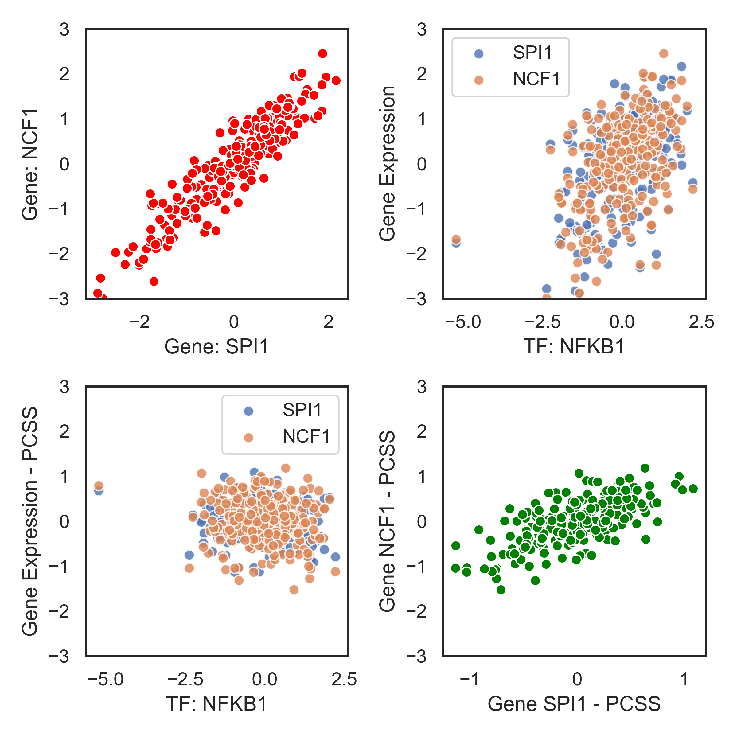
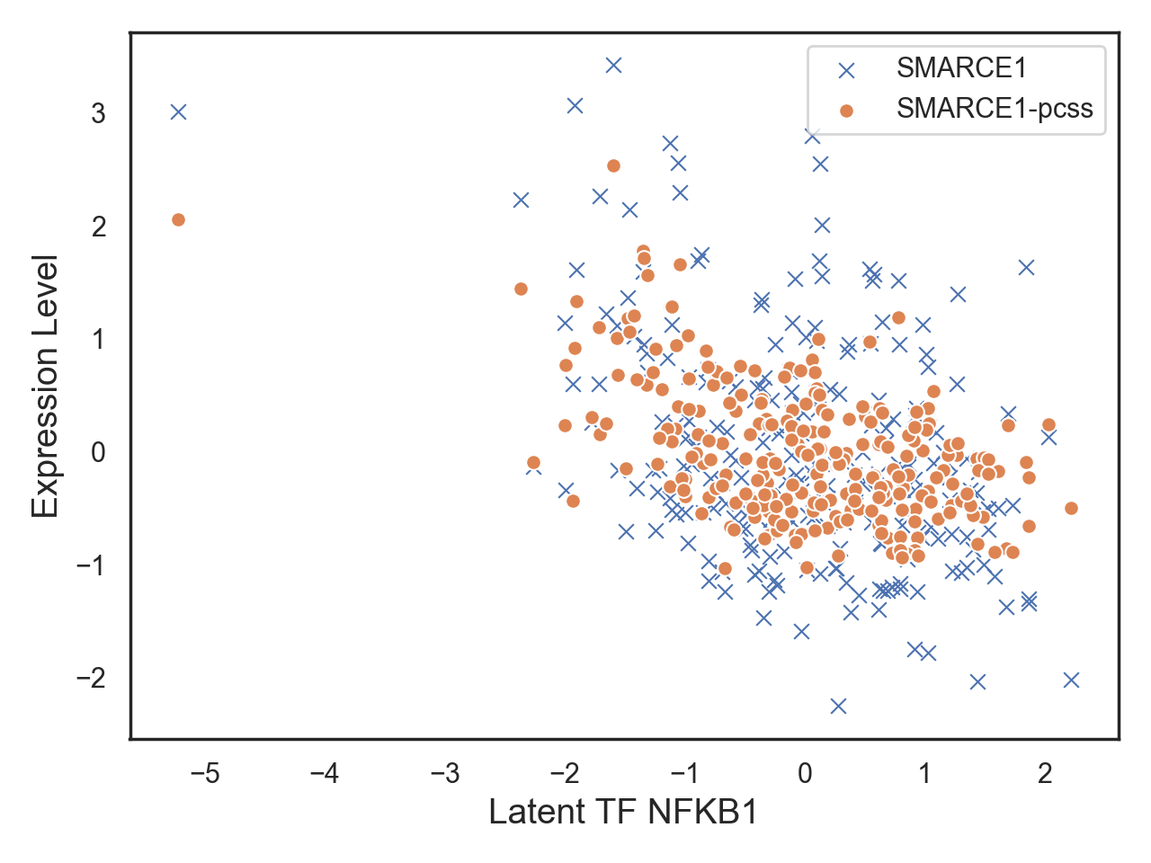
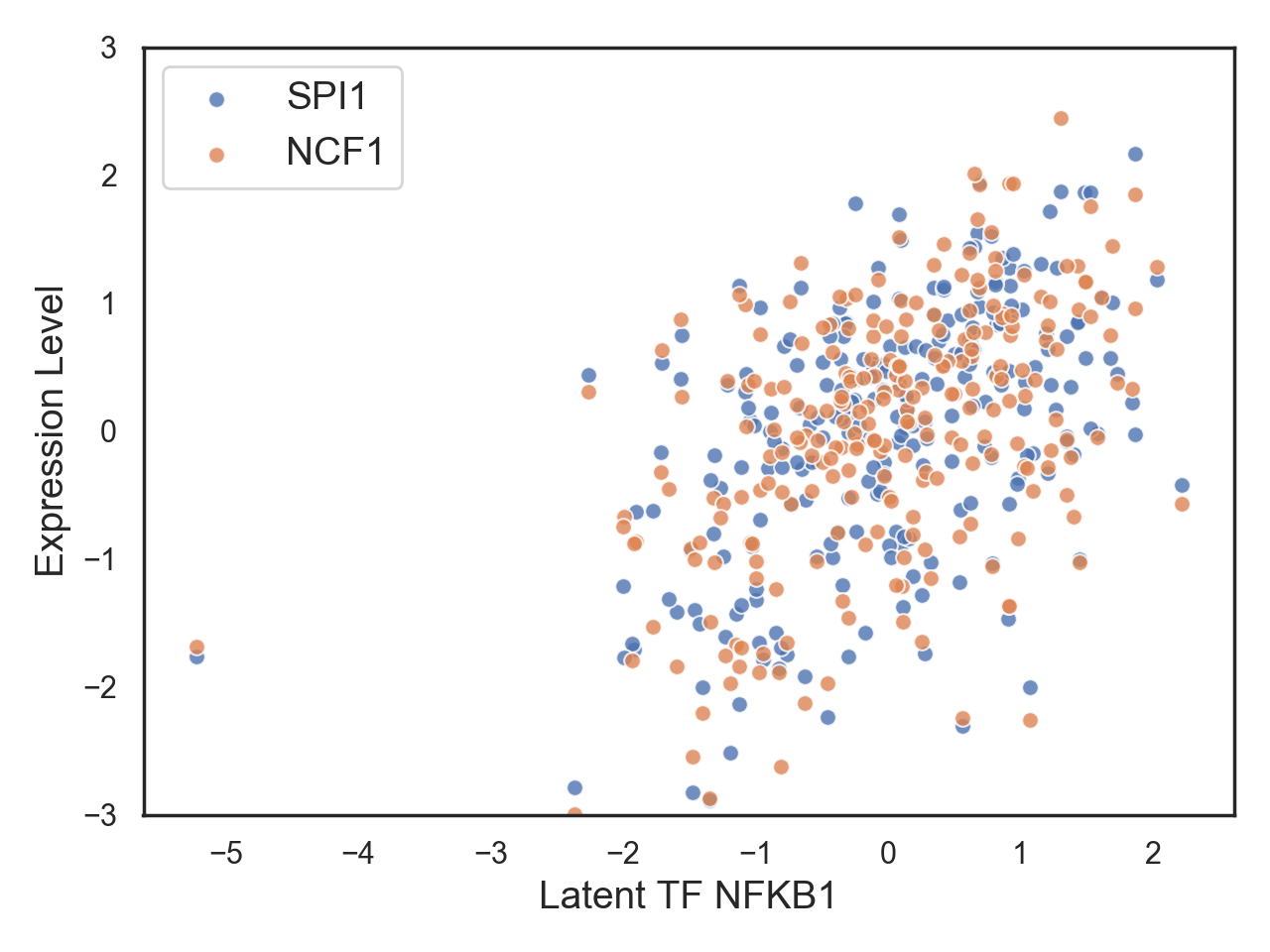
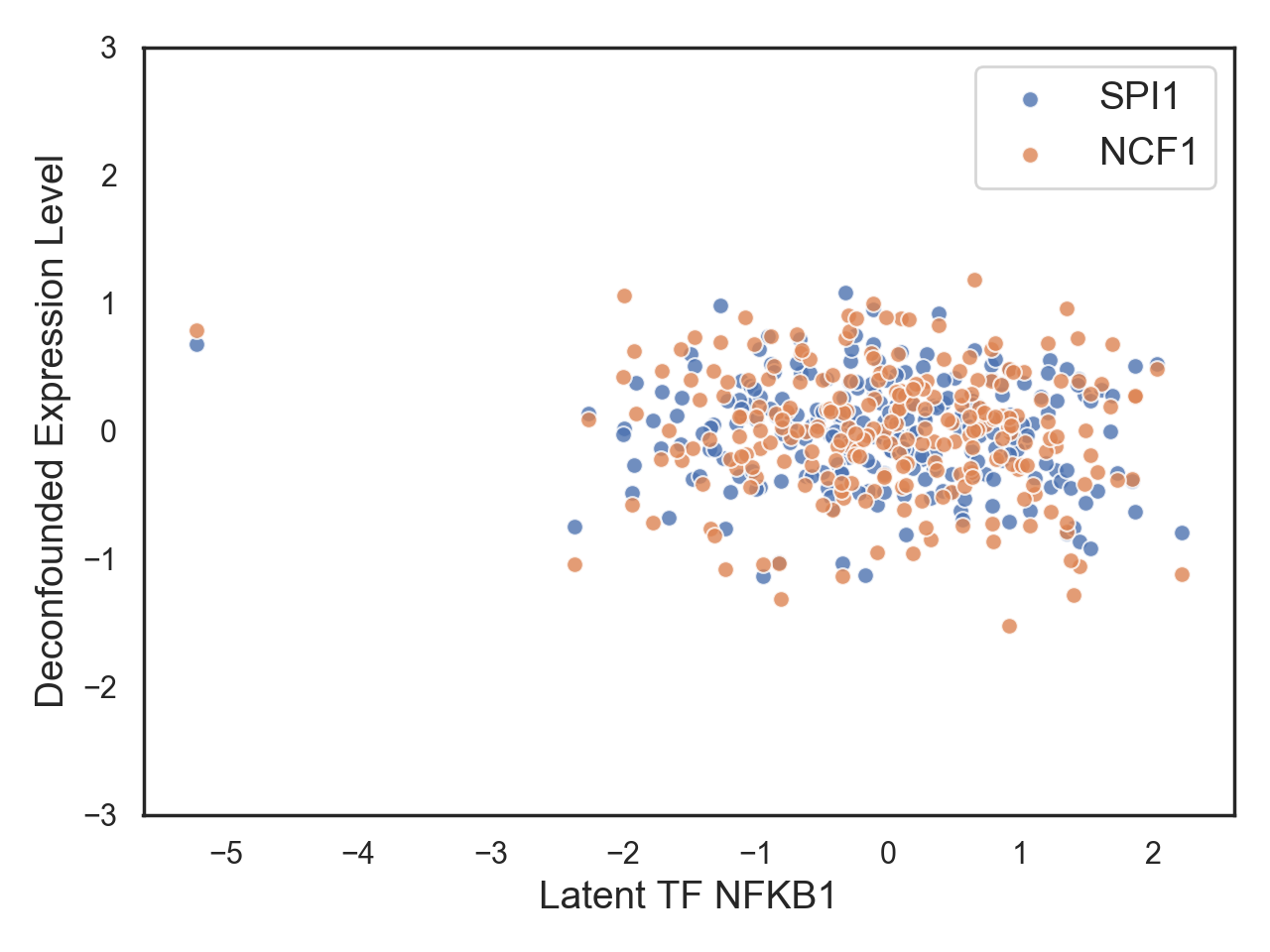
By removing the TFs, we can evaluate the methods in a similar fashion as the simulated experiments since we know the true values of the TFs. In the following, we first assess our ability to estimate the confounder sufficient statistics. Suppose that an observed gene $X_{j}$ is strongly correlated with one of the 15 latent TFs $T_{k}$, for some $1\leq j\leq 486$ and $1\leq k\leq 15$. Then, $\mathbb{E}[X_{j}\mid T_{k}]\approx\mathbb{E}[X_{j}\mid H]=S_{j}$. Since we know $T_{k}$, we can produce a similar plot as in Fig. 3. To this end, we look at NFKB1, which is a transcription factor known to be associated with ovarian cancer (Harrington and Annunziata, 2019). In Fig. 6, we look at the highest positive and negatively correlated genes with NFKB1, which are BIRC3 and SMARCE1 respectively. We see that the estimated confounding variation for each gene estimated from PCSS correlates well with the unobserved transcription factor NFKB1. This strong correlation suggests that PCSS estimates the variation explained by the unobserved confounders well in this dataset.

Figure 8: The x-axis denotes the proportion of times a method scored the incorrect parent appended to the neighborhood set higher than just the neighborhood set of a node (our proxy for the true parent set). The y-axis denotes the proportion of times a method scored the full neighborhood set higher than the neighborhood set after removing out one of the neighbors. For LRPS, we provide the intermediate results for each covariance matrix outputted along its cross-validation path. The ‘x’ for LRPS corresponds to the performance of the covariance matrix selected based on cross-validation. We compute the positive likelihood ratio for each method which equals the ratio between our proxy for the true positive rate (y-axis) and false positive rate (x-axis). These ratios are as follows: Vanilla-BIC=.26, PCSS-BIC=.33, CAM=.42, CAM-OBS=.59, DeCAMFound= .72, LRPC+BIC=.12.

5.2.2 Parent Recovery Performance

Unlike in the simulated dataset experiments, we do not know the true causal graph. Thus, for the Wrong Parent Addition task and the Correct Parent Deletion task, we use the graph structure outputted by NetBox, as in Frot et al. (2019). In particular, for a node $X_{j^{\prime}}$, we let $P_{\text{correct}}$ be the neighbors of $X_{j^{\prime}}$ in the graph outputted by NetBox. For the Wrong Parent Addition task, we require a set of “spurious neighbors” of $X_{j^{\prime}}$. For this set, we take all variables $X_{r^{\prime}}$ such that $X_{j^{\prime}}$ and $X_{r^{\prime}}$ are conditionally independent given $P_{t}$ and the TFs, but are conditionally dependent given only $P_{\text{correct}}$. Then, we let $P_{t}=P_{\text{correct}}\cup\{X_{r}\}$ for $X_{r}$ picked randomly from this set.

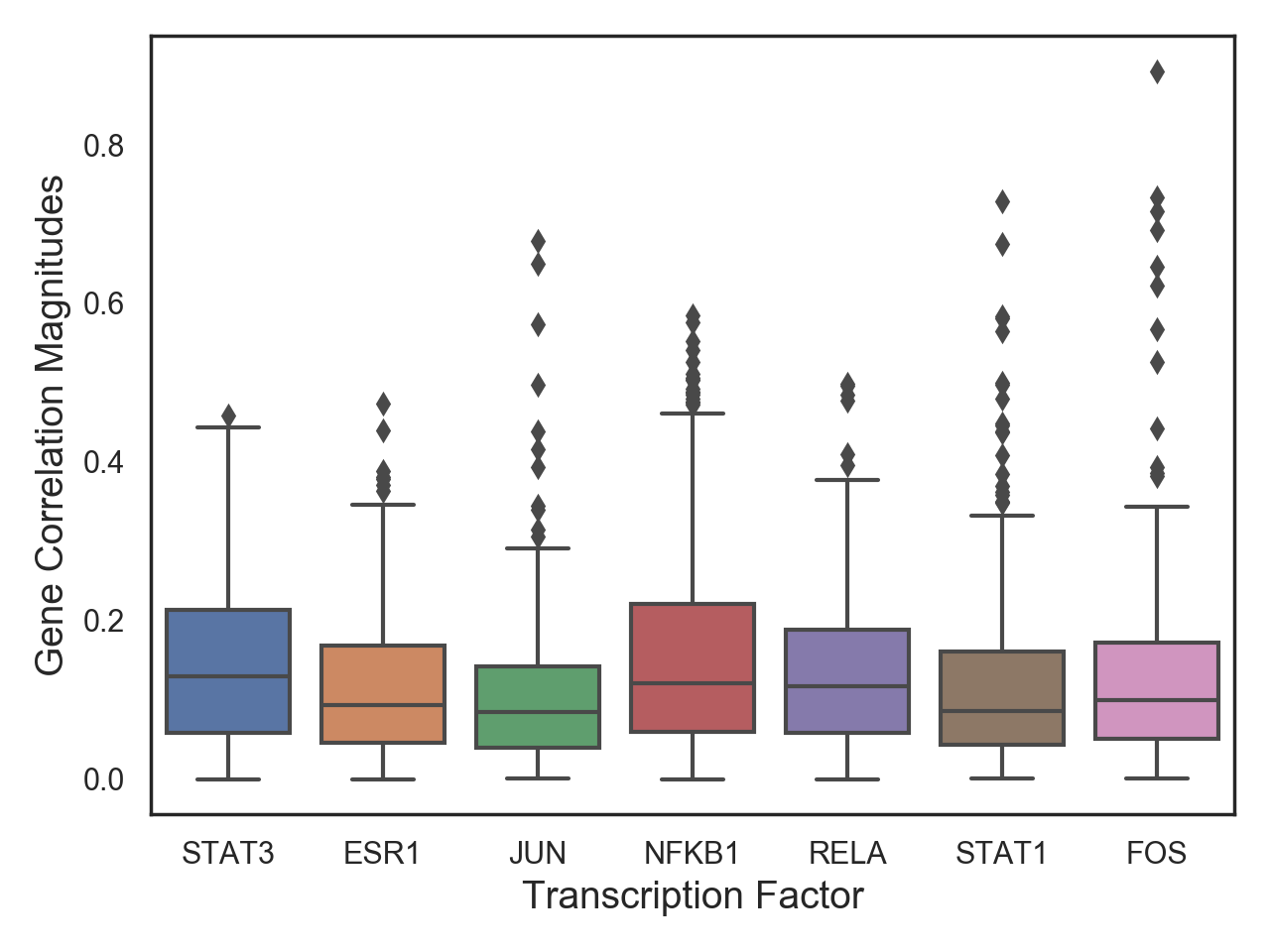
We focus on gene pairs $X_{j^{\prime}}$, $X_{r^{\prime}}$ with at least one strong TF confounder. In particular, we require that each gene has correlation greater than 0.4 with one of the 15 removed TFs. This choice makes it more likely that one of the 15 left-out TFs is the source of confounding, rather than some other unobserved confounder which we have no control over. This choice results in roughly 1000 parent sets to score. One such gene pair with a strong TF confounder is illustrated in Fig. 7. We see that subtracting the confounder sufficient statistics from each gene results in removing the confounding effect of the strongest transcription factor NFKB1.

For the Correct Parent Deletion task, we randomly sample 500 edges from the NetBox undirected graph. For each edge we randomly select one endpoint as $X_{j^{\prime}}$ and define $P_{t}=P_{\text{correct}}\setminus\{X_{r}\}$ for the other endpoint $X_{r}$.

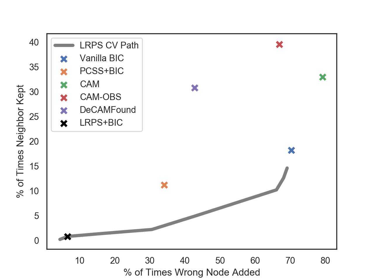
The results for both tasks are summarized in Fig. 8. LRPS produces a very sparse graph, and hence almost never adds a wrong parent. However, it almost always removes true edges, which comes at the expense of statistical power. Our method has the highest power per unit of false positives. Rather surprisingly, CAM-OBS, which explicitly uses the 15 held out transcription factors, selects wrong parents more often than our method. This might be the result of having additional (pervasive) confounders beyond the 15 TFs we introduced by design, as raised by Frot et al. (2019).

Conclusion. We have shown how to identify the causal graph among the observed nodes in the setting of non-linear effects and pervasive confounders. We proposed the DeCAMFounder, which consistently estimates a correct ordering of $\mathcal{G}^{*}$ using Gaussian processes. Since the DeCAMFounder explicitly accounts for confounders and non-linear effects, we found improved performance on both simulated and real datasets relative to existing methods. An interesting future direction is handling selection bias. In Frot et al. (2019), for example, the authors showed how to account for selection bias and pervasive confounders in the linear setting. It would be interesting to explore whether a similar idea could be used to extend the DeCAMFounder to handle selection bias.

Data and Code Availability. The simulated data, real data, and code used to generate our empirical results are available at https://github.com/uhlerlab/decamfound.

Acknowledgements We are thankful to the two referees, associate editor, and editor for their very helpful comments which led to an improved manuscript.

Funding. The authors were partially supported by NSF (DMS-1651995) and TRIPODS program (DMS-2022448), ONR (N00014-22-1-2116), the United States Department of Energy (DOE) Office of Advanced Scientific Computing Research (ASCR) via the M2dt MMICC center (DE-SC0023187), the MIT-IBM Watson AI Lab, the Eric and Wendy Schmidt Center at the Broad Institute, and a Simons Investigator Award to C. Uhler.

Conflict of Interest. None declared.

List of Figure Legends

Fig. 1

The right-hand figure reparameterizes the model on the left such that the unobserved variable $H$ is a source in the graph. The bold arrows represent the DAG $\mathcal{G}^{*}$ corresponding to the conditional distribution $\mathbb{Q}(X\mid H)$.

Fig. 2

Maximum Mean-Squared Error (MSE) across all dimensions for estimating $\{s^{(n)}\}_{n=1}^{N}$ via PCSS. Twenty-five total simulations were performed for each dataset configuration.

Fig. 3

Non-linear estimation of $E[X_{i}\mid H]$ via PCSS for nodes with at least one parent.

Fig. 4

Our parent set evaluation tasks. Solid arrows represent the set of true edges, and dotted arrows indicate a potential incorrect modifcation to the true parent set of a node.

Fig. 5

Results for the Wrong Parent Addition and Correct Parent Deletion tasks (lower values on the y-axis are better for both tasks). The data are generated according to a non-linear SEM. 25 total simulations per dataset configuration were performed.

Fig. 6

The two genes most positively and negatively correlated with the transcription factor NFKB1, respectively. GENE-pcss refers to the total latent confounding variation estimated for that gene via PCSS. GENE refers to the observed values of the gene.

Fig. 7

Both genes have a correlation greater than 0.4 with NFKB1 (left hand plot). After subtracting out the confounding variation estimated using PCSS for each gene (denoted as “deconfounded” expression level), the genes are no longer correlated with the unobserved transcription factor NFKB1.

Fig. 8

The x-axis denotes the proportion of times a method scored the incorrect parent appended to the neighborhood set higher than just the neighborhood set of a node (our proxy for the true parent set). The y-axis denotes the proportion of times a method scored the full neighborhood set higher than the neighborhood set after removing out one of the neighbors. For LRPS, we provide the intermediate results for each covariance matrix outputted along its cross-validation path. The ‘x’ for LRPS corresponds to the performance of the covariance matrix selected based on cross-validation. We compute the positive likelihood ratio for each method which equals the ratio between our proxy for the true positive rate (y-axis) and false positive rate (x-axis). These ratios are as follows: Vanilla-BIC=.26, PCSS-BIC=.33, CAM=.42, CAM-OBS=.59, DeCAMFound= .72, LRPC+BIC=.12.

Supplementary Material

Appendix A Notation

In the following table, we provide an overview of the main notations used in the paper.

Random Variables
$X$	Observed random vector, with dimension $p$	Eq. 2
$H$	Unobserved random vector, with dimension $K$	Eq. 2
$\epsilon$	Exogenous noise variables	Eq. 2
$S$	Confounder sufficient statistics $\mathbb{E}[X\mid H]$	Section 3.1
$U$	Component of $X$ orthogonal to $\mathcal{H}_{M}$	Section 3.2
Distributions
$\mathbb{P}$	Marginal distribution over $X$	Eq. 2
$\mathbb{Q}$	Joint distribution over $X,H$	Eq. 2
Graphs
$\mathcal{G}^{*}$	Conditional DAG associated with $\mathbb{Q}(X\mid H)$	Eq. 2
$\overline{\mathcal{G}}$	Full DAG over $X,H$	Eq. 2
$\textnormal{Pa}_{\mathcal{G}}^{j}$	Parents of $X_{j}$ in $\mathcal{G}$	Eq. 2
$\textnormal{An}_{\mathcal{G}}^{j}$	Ancestors of $X_{j}$ in $\mathcal{G}$	Section 3.3
$\mathfrak{G}$	Set of possible DAGs	Section 3.3
Data
$N$	Number of samples	Eq. 2
$p$	Number of observed nodes	Eq. 2
$\mathbb{X}$	Matrix of samples, $\in\mathbb{R}^{N\times p}$	Section 3.2
$\mathbb{S}$	Matrix of confounder sufficient statistics, $\in\mathbb{R}^{N\times p}$	Section 3.2
$\mathbb{U}$	$\in\mathbb{R}^{N\times p}$	Section 3.2
Function Spaces
$\mathcal{H}$	Hilbert space containing $X_{j}$	Section 3.2
$M$	Dimensionality of $\mathcal{H}$	Section 3.2
$\Phi$	Feature map on $H$	Section 3.2
$\tilde{\mathcal{F}}_{j}$	RKHS used to model $f_{ij}$, $1\leq j\leq p$	Section 3.2
$\tilde{\mathcal{R}}_{j}$	RKHS used to model $r_{j}$, $1\leq j\leq p$	Section 3.2

Appendix B Proofs

B.1 The canonical exogenous DAG

We provide a brief argument to verify that our direct definition of the canonical exogenous DAG is equal to the canonical DAG of the latent projection defined by Evans (2016). Our direct definition allows us to avoid the concepts of simplicial complexes and facets that are necessary to define the latent projection; see Evans (2016) for details.

Proposition 2.

Let $\bar{\mathcal{G}}$ be a DAG over observed nodes $X$ and unobserved nodes $\bar{H}$. Let $\mathcal{G}_{1}$ be the canonical exogenous DAG for $\bar{\mathcal{G}}$. Let $\mathcal{G}^{\prime}$ be the latent projection of $\mathcal{G}$ onto $X$, and let $\mathcal{G}_{2}$ be the canonical DAG associated with $\mathcal{G}^{\prime}$. Then $\mathcal{G}_{1}=\mathcal{G}_{2}$.

Proof.

By definition of the latent projection, $\mathcal{G}^{\prime}$ contains $X_{i}\to X_{j}$ if and only if $X_{i}$ has a completely hidden path to $X_{j}$. Furthermore, by definition of the canonical DAG, $\mathcal{G}_{2}$ contains an edge $X_{i}\to X_{j}$ if and only if $\mathcal{G}^{\prime}$ contains the edge $X_{i}\to X_{j}$. Thus, $\mathcal{G}_{1}$ and $\mathcal{G}_{2}$ have the same set of edges over $X$.

Next, $\mathcal{G}^{\prime}$ contains the bidirected face $C$ if and only if the nodes $X_{C}$ share a hidden common cause. Furthermore, $\mathcal{G}_{2}$ contains the node $H_{k}$ if and only if $C_{k}$ is a bidirected facet in $\mathcal{G}^{\prime}$, i.e., if $X_{C}$ is a maximal set of nodes with a hidden common cause. In this case, $\mathcal{G}_{2}$ has the edge $H_{k}$ to $X_{i}$ if and only if $i\in C$. Thus, $\mathcal{G}_{1}$ and $\mathcal{G}_{2}$ have the same set of edges from $H$ to $X$.

By both constructions, there are no edges from $X$ to $H$ or between nodes in $H$, thus, $\mathcal{G}_{1}$ and $\mathcal{G}_{2}$ are equal. ∎

B.2 Proof of 1

Proof.

By Eq. 2,

$$X=(I-B)^{-1}\epsilon+(I-B)^{-1}\Theta H.$$ (11)

Hence, for all $1\leq j\leq p$,

$$\begin{split}X_{j}&=\sum_{i\in\textnormal{Pa}_{\mathcal{G}^{*}}^{j}}B_{ij}X_{i}+\Theta_{i}^{T}H\\ &=\sum_{i\in\textnormal{Pa}_{\mathcal{G}^{*}}^{j}}B_{ij}[(I-B)^{-1}\epsilon+(I-B)^{-1}\Theta H]_{i}+\Theta_{j}^{T}H.\end{split}$$ (12)

Taking expectations with respect to $H$,

$$\begin{split}S_{j}&=\mathbb{E}[X_{j}\mid H]\\ &=\mathbb{E}\left[\sum_{i\in\textnormal{Pa}_{\mathcal{G}^{*}}^{j}}B_{ij}[(I-B)^{-1}\epsilon+(I-B)^{-1}\Theta H]_{i}+\Theta_{j}^{T}H\mid H\right]\\ &=\sum_{i\in\textnormal{Pa}_{\mathcal{G}^{*}}^{j}}\mathbb{E}\left[B_{ij}[(I-B)^{-1}\epsilon+(I-B)^{-1}\Theta H]_{i}\mid H\right]+\Theta_{j}^{T}H\\ &=\sum_{i\in\textnormal{Pa}_{\mathcal{G}^{*}}^{j}}[(I-B)^{-1}\Theta H]_{i}+\Theta_{j}^{T}H\qquad(\text{since $\epsilon\perp\!\!\!\perp H$}),\end{split}$$ (13)

where $[a]_{i}$ denotes the $i$th component of a vector $a$. Let $\Theta_{j,:}$ denote the $j$th row of $\Theta$. Recalling that $D_{j}=\Theta_{j,\cdot}^{T}\,H=S_{j}-r_{j}(S_{1},\cdots,S_{j-1})$,

$$\begin{split}r_{j}(S_{1},\cdots,S_{j-1})&=\sum_{i\in\textnormal{Pa}_{\mathcal{G}^{*}}^{j}}B_{ij}[(I-B)^{-1}\Theta H]_{i}.\\ &=\sum_{i\in\textnormal{Pa}_{\mathcal{G}^{*}}^{j}}B_{ij}S_{i}\quad\text{(by \lx@cref{creftype~refnum}{eq:linear_s})}.\end{split}$$ (14)

Therefore, the SCM in Eq. 2 can be re-written as

$$(X_{j}-S_{j})=\sum_{i\in\textnormal{Pa}_{\mathcal{G}^{*}}^{j}}B_{ij}(X_{i}-S_{i})+\epsilon_{j}.$$ (15)

∎

B.3 Proof of 1

Lemma 2.

For every $1\leq j\leq p$, there exists an $f_{j}$ such that

$$X_{j}=\epsilon_{j}+D_{j}+f_{j}(\epsilon_{1},D_{1},\cdots,\epsilon_{j-1},D_{j-1})$$ (16)

for the SEM in Eq. 1.

Proof.

The proof follows by inducting on the number of nodes in $\mathcal{G}^{*}$. For $p=1$, $X_{1}=D_{1}+\epsilon_{2}$, and Eq. 16 trivially holds. For $p=2$,

$$\begin{split}X_{2}&=D_{2}+\epsilon_{2}+f_{12}(X_{1})\\ &=D_{2}+\epsilon_{2}+f_{12}(D_{1}+\epsilon_{1}).\end{split}$$ (17)

The claim holds by setting $f_{2}(\epsilon_{1},d_{1})=f_{12}(d_{1}+\epsilon_{1})$. Suppose that Eq. 16 holds for all DAGs with at most $p-1$ nodes. Then it suffices to prove that Eq. 16 holds for all DAGs with $p$ nodes. For this, note that

$$\begin{split}X_{p}&=D_{p}+\epsilon_{p}+\sum_{i\in\textnormal{Pa}_{\mathcal{G}^{*}}^{p}}f_{ij}(X_{i})\\ &=D_{p}+\epsilon_{p}+\sum_{i\in\textnormal{Pa}_{\mathcal{G}^{*}}^{p}}f_{ij}(\epsilon_{i}+D_{i}+f_{j}(\epsilon_{1},D_{1},\cdots,\epsilon_{i-1},D_{i-1})),\end{split}$$ (18)

where the last line follows from the inductive hypothesis. Thus, by setting

$$f_{p}(\epsilon_{1},d_{1},\cdots,\epsilon_{j-1},d_{p-1})=\sum_{i\in\textnormal{Pa}_{\mathcal{G}^{*}}^{p}}f_{ij}(\epsilon_{i}+d_{i}+f_{j}(\epsilon_{1},d_{1},\cdots,\epsilon_{i-1},d_{i-1})),$$

the claim follows. ∎

Corollary 3.

For an SEM in the form of Eq. 1, it holds that

$$\mathbb{E}[X_{j}\mid H]=\mathbb{E}[X_{j}\mid D_{1},\cdots,D_{j}].$$

We prove 1 below using 3.

Proof.

By Eq. 1, it suffices to show that there exists an $r_{j}$ such that $D_{j}=S_{j}-r_{j}(S_{1},\cdots,S_{j-1})$ for every $1\leq j\leq p$. We prove this claim by inducting on the number of nodes in $\mathcal{G}^{*}$. For $p=1$, $X_{1}=D_{1}+\epsilon_{1}$. Since $H\perp\!\!\!\perp\epsilon$, $S_{1}=D_{1}$, and the claim holds by setting $R_{1}=0$. For $p=2$, $X_{2}=\epsilon_{2}+D_{2}+f_{12}(X_{1})$, where $f_{12}$ may equal $0$ if $X_{1}$ is not a parent of $X_{2}$. Then,

$$\begin{split}S_{2}&=\mathbb{E}[X_{2}\mid H]\\ &=\mathbb{E}[X_{2}\mid D_{1},D_{2}]\quad\text{(by \lx@cref{creftype~refnum}{cor:suff_dir_confound}})\\ &=\mathbb{E}[D_{2}+\epsilon_{2}+f_{12}(X_{1})\mid D_{1},D_{2}]\\ &=D_{2}+\mathbb{E}[f_{12}(X_{1})\mid D_{1}]\\ &=D_{2}+\mathbb{E}[f_{12}(X_{1})\mid S_{1}]\quad\text{(since $S_{1}=D_{1}$)}.\end{split}$$ (19)

Hence, $D_{2}=S_{2}-\mathbb{E}[f_{12}(X_{1})\mid S_{1}]$. The claim holds by setting $r_{2}(S_{1})=\mathbb{E}[f_{12}(X_{1})\mid S_{1}]$. Suppose that $D_{j}=S_{j}-r_{j}(S_{1},\ldots,S_{j-1})$ for all SEMs in the form of Eq. 1 with at most $p-1$ nodes. It suffices to show that that there exists an $r_{p}$ such that $d_{p}=s_{p}-r_{p}(s_{1},\ldots,s_{p-1})$ for an arbitrary SEM in the form of Eq. 1 with $p$ nodes.

For this, consider the subgraph formed from $x_{1},\ldots,x_{p-1}$. Since $X_{p}$ is a sink node, $\mathbb{Q}(X_{1},\ldots,X_{p-1})$ factorizes according to a DAG. Hence, by the inductive hypothesis, there exists $\{r_{j}\}_{j=1}^{p-1}$ such that

$$D_{j}=S_{j}-r_{j}(S_{1},\ldots,S_{j-1})\quad\forall j=1,\ldots,p-1.$$ (20)

Now, note that

$$\begin{split}S_{p}&=\mathbb{E}[X_{p}\mid H]\\ &=\mathbb{E}[X_{p}\mid D_{1},D_{2},\ldots,D_{p}]\quad\text{(by \lx@cref{creftype~refnum}{cor:suff_dir_confound}})\\ &=\mathbb{E}\left[D_{p}+\epsilon_{p}+\sum_{i\in\textnormal{Pa}_{\mathcal{G}^{*}}^{p}}f_{ij}(X_{i})\mid D_{1},D_{2},\ldots,D_{p}\right]\\ &=D_{p}+\mathbb{E}\left[\sum_{i\in\textnormal{Pa}_{\mathcal{G}^{*}}^{p}}f_{ij}(X_{i})\mid D_{1},D_{2},\cdots,D_{p-1}\right]\\ &=D_{p}+\mathbb{E}\left[\sum_{i\in\textnormal{Pa}_{\mathcal{G}^{*}}^{p}}f_{ij}(X_{i})\mid\{S_{i}-r_{i}(S_{1},\cdots,S_{i-1})\}_{i=1}^{p-1}\right]\quad\text{(by \lx@cref{creftype~refnum}{eq:induct_hyp})}.\end{split}$$ (21)

Thus, by setting

$$r_{p}(s_{1},\cdots,s_{p-1})=\mathbb{E}\left[\sum_{x_{i}\in\textnormal{Pa}_{\mathcal{G}^{*}}^{p}}f_{ij}(X_{i})\mid\{s_{i}-r_{i}(s_{1},\cdots,s_{i-1})\}_{i=1}^{p-1}\right],$$ (22)

the result follows. ∎

B.4 Proof of 2

We use a subset of the technical assumptions from Section 3 of Fan et al. (2013) to prove the result. We let $\Sigma_{u}=\text{Cov}(U)\in\mathbb{R}^{p\times p}$, where $U$ is defined in Eq. 4. In this section, we work with the joint distribution over $N$ samples. In particular, we consider a sequence of random vectors $(X^{(1)},H^{(1)}),\ldots,(X^{(N)},H^{(N)})$, whose joint distribution is the product distribution over $N$ copies of $\mathbb{Q}(X,H)$.

Assumption 6.

(Assumption 2(c) from Fan et al. (2013)) There exist constants $r_{1},r_{2}>0$ and $b_{1},b_{2}>0$, such that for any $q>0$, $1\leq j\leq p$ and $1\leq m\leq M$,

$$\mathbb{Q}(|U_{j}|>q)\leq\exp\{(-q/b_{1})^{r_{1}}\},\qquad\mathbb{Q}(|\phi_{m}(H)|>q)\leq\exp\{(-q/b_{2})^{r_{2}}\}$$

As discussed in Fan et al. (2013), 6 requires exponential-type tails for the purposes of applying large deviation theory. Fan et al. (2013) also states, in their working paper, that $\|\Sigma_{u}\|_{1}<c_{2}$ in 3 can be weakened to just requiring that $\lambda_{max}(\Sigma_{u})<c_{2}$ if the number of factors $J$ to use in PCA is known. The final assumption below bounds the strength of the latent factor loadings in $\Psi$, and the convergence of $[u^{(n)}]^{T}u^{(t)}$ towards its expectation.

Assumption 7.

(Assumption 4 from Fan et al. (2013)) There exists a constant $C>0$ such that for all $1\leq j\leq p$, $1\leq n,t\leq N$:

1. $\max_{1\leq m\leq M}[\psi_{j}]_{m}<C$,

2. $\mathbb{E}\left[p^{-1/2}\left([U^{(n)}]^{T}U^{(t)}-\mathbb{E}[[U^{(n)}]^{T}U^{(t)}]\right)\right]^{4}<C$

3. $\mathbb{E}\|p^{-1/2}\sum_{j=1}^{p}\Psi_{j}U_{j}^{(n)}\|^{4}<M$.

By Corollary 1 of Fan et al. (2013), it suffices to show that Assumption 2(a) and Assumption 3 in Fan et al. (2013) hold. For $1\leq j\leq p$,

$$\begin{split}\mathbb{E}[U_{j}]&=\mathbb{E}[X_{j}-\mathbb{E}[X_{j}\mid H]]\\ &=\mathbb{E}[X_{j}]-\mathbb{E}[\mathbb{E}[X_{j}\mid H]]\\ &=0.\end{split}$$

By properties of conditional expectation, $U_{j}$ belongs to the orthogonal complement of $\mathcal{H}_{M}$. Hence, $\mathbb{E}[U_{j}\phi_{m}(H)]=0$ for all $1\leq j\leq p$. Thus, Assumption 2(a) holds. Since $\{(x^{(n)},h^{(n)})\}_{n=1}^{N}$ are drawn iid from $\mathbb{Q}$, then $(X^{(n)},H^{(n)})$ is independent of $(X^{(t)},H^{(t)})$ when $n\neq t$. Hence, the strong-mixing coefficient defined in Equation 3.1 of Fan et al. (2013) equals 0. Therefore, Assumption 3 in Fan et al. (2013) indeed holds.

B.5 Proof of 1

We follow Friedman and Nachman (2000) to compute the marginal likelihood. By 1, the marginal likelihood decomposes as

$$\begin{split}\mathbb{Q}(\mathbb{X}\mid\mathcal{G},\mathbb{S},\sigma^{2})&=\int\mathbb{Q}(\mathbb{X}\mid\mathcal{G},\mathbb{S},\Omega_{\mathcal{G}},\sigma^{2})d\mathbb{Q}(\Omega_{\mathcal{G}}\mid\mathcal{G})\\ &=\int\prod_{j=1}^{p}\mathbb{Q}(\mathbb{X}_{:,j}-\mathbb{S}_{:,j}\mid\mathbb{X}_{\textnormal{Pa}_{\mathcal{G}}^{j}},\mathbb{S},\{f_{ij}\}_{i\in\textnormal{Pa}_{\mathcal{G}}^{j}},r_{j},\sigma^{2})d\mathbb{Q}(\{f_{ij}\}_{i\in\textnormal{Pa}_{\mathcal{G}}^{j}},r_{j})\\ &=\prod_{j=1}^{p}\int\mathbb{Q}(\mathbb{X}_{:,j}-\mathbb{S}_{:,j}\mid\mathbb{X}_{\textnormal{Pa}_{\mathcal{G}}^{j}},\mathbb{S},\{f_{ij}\}_{i\in\textnormal{Pa}_{\mathcal{G}}^{j}},r_{j},\sigma^{2})d\mathbb{Q}(\{f_{ij}\}_{i\in\textnormal{Pa}_{\mathcal{G}}^{j}},r_{j})\\ &=\prod_{j=1}^{p}\mathbb{Q}(\mathbb{X}_{:,j}-\mathbb{S}_{:,j}\mid\mathbb{X}_{\textnormal{Pa}_{\mathcal{G}}^{j}},\mathbb{S},\sigma^{2}).\end{split}$$

Hence,

$$\log\mathbb{Q}(\mathbb{X}\mid\mathcal{G},\mathbb{S},\sigma^{2})=\sum_{j=1}^{p}\log\mathbb{Q}(\mathbb{X}_{:,j}-\mathbb{S}_{:,j}\mid\mathbb{X}_{\textnormal{Pa}_{\mathcal{G}}^{j}},\mathbb{S},\sigma^{2}).$$

The proof now follows from Equation 2.30 of Rasmussen and Williams (2006).

B.6 Proof of 3

Notation. Throughout we let $\|\mathbf{a}\|_{N}^{2}=\frac{1}{N}\sum_{n=1}^{N}(a^{(n)})^{2}$ denote the empirical norm of a vector $\mathbf{a}\in\mathbb{R}^{N}$, and $\mathbb{Q}_{N}$ the empirical distribution of $\{(x^{(n)},s^{(n)})\}_{n=1}^{N}$. For simplicity of notation, we assume that, for all $1\leq j\leq p$ and $i\in\textnormal{Pa}_{\mathcal{G}}^{j}$, we have $\tilde{\mathcal{F}}_{ij}=\tilde{\mathcal{F}}_{j}$ for some $\tilde{\mathcal{F}}_{j}$. We denote the maximum likelihood estimate (MLE) of the noise variances and unknown functions in $\Omega_{G}$ when using the confounder sufficient statistics $\hat{s}$ estimated from Algorithm 1 as

$$\begin{split}&(\hat{\sigma}_{j}^{\mathcal{G}})^{2}\coloneqq\left\|x_{j}-\sum_{i\in\textnormal{Pa}_{\mathcal{G}}^{j}}\hat{f}_{ij}^{\mathcal{G}}(x_{i})-\hat{s}_{j}+\hat{r}_{j}^{\mathcal{G}}(\hat{s}_{\textnormal{Pa}_{\mathcal{G}}^{j}})\right\|_{N}^{2}\\ \{\hat{f}_{ij}^{\mathcal{G}}\}_{i\in\textnormal{Pa}_{\mathcal{G}}^{j}},\hat{r}_{j}^{\mathcal{G}}=&\operatorname*{arg\,min}_{\ g_{ij}\in\tilde{\mathcal{F}}_{j},\ w_{j}\in\tilde{\mathcal{R}}_{j}^{\mathcal{G}}}\left\|x_{j}-\sum_{i\in\textnormal{Pa}_{\mathcal{G}}^{j}}g_{ij}(x_{i})-\hat{s}_{j}-w_{j}(\hat{s}_{\textnormal{Pa}_{\mathcal{G}}^{j}})\right\|^{2}_{N}\end{split}$$ (23)

for $1\leq j\leq p$. When the true confounder sufficient statistics $s$ are used instead of $\hat{s}$, we let

$$\begin{split}&(\bar{\sigma}_{j}^{\mathcal{G}})^{2}\coloneqq\left\|x_{j}-\sum_{i\in\textnormal{Pa}_{\mathcal{G}}^{j}}\bar{f}_{ij}^{\mathcal{G}}(x_{i})-s_{j}+\bar{r}_{j}^{\mathcal{G}}(s_{\textnormal{Pa}_{\mathcal{G}}^{j}})\right\|_{N}^{2}\\ \{\bar{f}_{ij}^{\mathcal{G}}\}_{i\in\textnormal{Pa}_{\mathcal{G}}^{j}},\bar{r}_{j}^{\mathcal{G}}=&\operatorname*{arg\,min}_{\ g_{ij}\in\tilde{\mathcal{F}}_{j},\ m_{j}\in\tilde{\mathcal{R}}_{j}^{\mathcal{G}}}\left\|x_{j}-\sum_{i\in\textnormal{Pa}_{\mathcal{G}}^{j}}g_{ij}(x_{i})-s_{j}-m_{j}(s_{\textnormal{Pa}_{\mathcal{G}}^{j}})\right\|^{2}_{N}.\end{split}$$ (24)

denote the corresponding maximum likelihood estimates for $1\leq j\leq p$. Finally, for ease of notation later on, we let

$$\begin{split}h^{\mathcal{G}}_{j}(x_{\textnormal{Pa}_{\mathcal{G}}^{j}},s_{\textnormal{Pa}_{\mathcal{G}}^{j}})&=\sum_{i\in\textnormal{Pa}_{\mathcal{G}}^{j}}f_{ij}^{\mathcal{G}}(x_{i})-s_{j}+r_{j}^{\mathcal{G}}(s_{\textnormal{Pa}_{\mathcal{G}}^{j}})\\ \hat{h}^{\mathcal{G}}_{j}(x_{\textnormal{Pa}_{\mathcal{G}}^{j}},\hat{s}_{\textnormal{Pa}_{\mathcal{G}}^{j}})&=\sum_{i\in\textnormal{Pa}_{\mathcal{G}}^{j}}\hat{f}_{ij}^{\mathcal{G}}(x_{i})-\hat{s}_{j}+\hat{r}_{j}^{\mathcal{G}}(\hat{s}_{\textnormal{Pa}_{\mathcal{G}}^{j}})\\ \bar{h}^{\mathcal{G}}_{j}(x_{\textnormal{Pa}_{\mathcal{G}}^{j}},s_{\textnormal{Pa}_{\mathcal{G}}^{j}})&=\sum_{i\in\textnormal{Pa}_{\mathcal{G}}^{j}}\bar{f}_{ij}^{\mathcal{G}}(x_{i})-s_{j}+\bar{r}_{j}^{\mathcal{G}}(s_{\textnormal{Pa}_{\mathcal{G}}^{j}}).\end{split}$$ (25)

for $1\leq j\leq p$. To establish a uniform law of large numbers, we will make use of the following result from Wainwright (2019).

Lemma 3.

(Exercise 2.12 in Wainwright (2019)) Let $\{X_{i}\}_{i=1}^{n}$ be a sequence of zero-mean random variables, each sub-Gaussian with parameter $\sigma$. Then, for $\delta>0$,

$$\mathbb{P}\left(\max_{i=1,\cdots,n}|X_{i}|\geq 2\sigma\sqrt{\log 2n}+\delta\right)\leq 2\exp\left(-\frac{\delta^{2}}{2\sigma^{2}}\right).$$

Discussion of Additional Assumptions.

Assumption 8.

(sparsity condition) There exists a constant $\gamma<\infty$ such that $\mathcal{G}^{*}\in\mathfrak{G}$ for all $p$, where $\mathfrak{G}=\{\mathcal{G}:|\textnormal{Pa}_{\mathcal{G}}^{i}|\leq\gamma\}$.

Assumption 9.

(Function class behavior) Let $\tilde{\mathcal{F}}_{j}^{\mathcal{G}}=\bigoplus_{i\in\textnormal{Pa}_{\mathcal{G}}^{i}}\tilde{\mathcal{F}}_{i}$, $1\leq j\leq p$, and assume all constants $\{C_{i}\}_{i=1}^{6}$ below do not depend on $p$ and are less than $\infty$.

1. There exists a constant $C_{1}$ such that for all $G\in\mathfrak{G}$, $\mathrm{rank}(\tilde{\mathcal{F}}_{j})\leq C_{1}$ and $\mathrm{rank}(\tilde{\mathcal{R}}_{j}^{\mathcal{G}})\leq C_{1}$ for all $1\leq j\leq p$ and $G\in\mathfrak{G}$.

2. There exists a constant $C_{2}$ such that

   $$\max_{G\in\mathfrak{G}}H\left(u,\tilde{\mathcal{F}}_{j}^{\mathcal{G}}\bigoplus\tilde{\mathcal{R}}_{j}^{\mathcal{G}},L^{1}(\mathbb{Q})\right)<C_{2},\quad\max_{G\in\mathfrak{G}}H\left(u,\tilde{\mathcal{F}}_{j}^{\mathcal{G}}\bigoplus\tilde{\mathcal{R}}_{j}^{\mathcal{G}},L^{4}(\mathbb{Q})\right)<C_{2},$$

   for all $1\leq j\leq p$ and $u>0$, where $H$ is the log-bracketing number of the function class with respect to the $L_{1}$ and $L_{4}$ norms, and $u>0$ denotes the largest distance between any two functions in the bracketing of the function class.

3. There exists a constant $C_{3}$ such that for $1\leq j\leq p$ the following quantities are all bounded above by $C_{3}$:

   $$\mathbb{E}|X_{j}|^{4},\quad\mathbb{E}|S_{j}|^{4},\quad\sup_{f\in\tilde{\mathcal{F}}_{j}}\mathbb{E}|f(X_{j})|^{4},\quad\max_{\mathcal{G}\in\mathfrak{G}}\sup_{r\in\tilde{\mathcal{R}}_{j}^{\mathcal{G}}}\mathbb{E}|r(S_{\textnormal{Pa}_{\mathcal{G}}^{j}})|^{4}.$$

4. There exists constants $C_{5}$ and $C_{6}$ such that

   $$\max_{1\leq j\leq p}\max_{\mathcal{G}\in\mathfrak{G}}\sup_{v_{j}^{\mathcal{G}}\in\tilde{\mathcal{F}}_{j}^{\mathcal{G}}\bigoplus\tilde{\mathcal{R}}_{j}^{\mathcal{G}}}\rho(m_{j}^{\mathcal{G}})\leq C_{4},\ \rho(M_{j}^{\mathcal{G}})=2C_{5}\mathbb{E}_{\mathbb{Q}}[\exp(|M_{j}^{\mathcal{G}}|/C_{5})-1-|M_{j}^{\mathcal{G}}|/C_{5}],$$

   where $M_{j}^{\mathcal{G}}=(X_{j}-S_{j}-v_{j}^{\mathcal{G}}(X_{\textnormal{Pa}_{\mathcal{G}}^{j}},S_{\textnormal{Pa}_{\mathcal{G}}^{j}}))^{2}$.

5. There exists a constant $C_{5}$ such that $\|\nabla r\|_{2}\leq C_{6}$ for all $r\in\tilde{\mathcal{R}}_{j}$, $1\leq j\leq p$.

6. There exists constants $0<C_{7},C_{8}<\infty$ such that

   $$\mathbb{Q}(||S_{j}|-\mathbb{E}[|S_{j}|]|>t)\leq C_{7}\exp(-C_{8}t^{2}),$$

   for all $1\leq j\leq p$.

Assumption 10.

There exists a constant $C_{4}$ such that $\min_{\mathcal{G}\in\mathfrak{G}}\min_{1\leq j\leq p}(\sigma_{j}^{\mathcal{G}})^{2}\geq C_{4}>0$.

In Bühlmann et al. (2014), the authors assume that the size of the neighborhood set of any observed node is uniformly bounded. Since the true parent set of a node is contained in its neighborhood set, 8 is a weaker condition. 5 and 9(a) together imply that the true DAG still has the smallest negative log-likelihood, even in the misspecified setting when $\tilde{\mathcal{F}}_{j}\subsetneq\mathcal{F}_{j}$. As shown in Bühlmann et al. (2014), if $\tilde{\mathcal{F}}_{j}$ is sufficiently close to $\mathcal{F}_{j}$ (i.e., by setting $C_{1}$ large enough), then assuming $\mathcal{G}^{*}$ still has the smallest negative log-likelihood over functions in $\tilde{\mathcal{F}}_{j}$ is weak. 9(b) is the analogue of Assumption B3(ii) in Bühlmann et al. (2014). Assumption B3(ii) in Bühlmann et al. (2014) is a smoothness assumption on the function class) used to prove that the log-bracketing number with respect to the $L^{4}$ norm is bounded. If we make the same smoothness assumption, then 9(b) holds by following the proof of Theorem 3 in Bühlmann et al. (2014). 9(c) and 9(d) (which assumes $m_{j}^{\mathcal{G}}$ has exponential moments) are also used in Bühlmann et al. (2014) to establish a uniform law of large numbers. 9(e) assumes that the function class $\tilde{\mathcal{R}}_{j}$ has bounded gradients, and 9(f) assumes that the confounder sufficient statistics are sub-Gaussian. 10 is a technical regularity assumption that ensures a log-likelihood exists (since the log of zero is undefined).

Proof of 3. A key difference between our consistency proof and the proof in Bühlmann et al. (2014) is accounting for the additional estimation error of estimating the confounder sufficient statistics $s$ via PCA. Once we bound the error in empirical log-likelihood scores when using $\hat{s}$ instead of $s$, our proof closely follows the proof of Theorem 3 in Bühlmann et al. (2014). Before we can follow the proof technique in Bühlmann et al. (2014), we show below that it suffices to prove the consistency of the MLE (a frequentist-based score) to prove consistency of the DeCAMFounder (a Bayesian-based score).

Reduction to Proving the Consistency of the MLE. The DeCAMFounder score of a DAG equals the sum of the marginal log-likelihood scores of each node. Under 9(a), each observed node belongs to a finite dimensional exponential family. Hence, by Haughton (1988), the marginal log-likelihood of the parent set $\textnormal{Pa}_{\mathcal{G}}^{j}$ for node $X_{j}$ converges to the negative BIC score of $\textnormal{Pa}_{\mathcal{G}}^{j}$. The BIC score equals the sum of empirical log-likelihood score associated with the MLE parameters in Eq. 23, and a penalty on model complexity which equals $\log N$ times the number of parameters. When a DAG $\mathcal{G}$ has a different partial ordering than $\mathcal{G}^{*}$, then the difference in expected log-likelihood between $\mathcal{G}$ and $\mathcal{G}^{*}$ is non-zero. Hence, the empirical log-likelihood scores grows as $O(N)$ while the penalty grows as $O(\log N)$. Since the log-likelihood score in BIC grows faster than the penalty, it suffices to show that minimizing the empirical negative log-likelihood of a DAG yields a DAG in $\Pi^{*}$ to prove order consistency of the DeCAMFounder.

Inequalities Sufficient for Proving Consistency. As we show below, if there exists a sufficient “gap” $\Delta_{N}$ (to be defined shortly) in empirical log-likelihood scores between the best incorrect DAG and the worst super-DAG of $\mathcal{G}^{*}$, then the DeCAMFounder converges to a DAG with a correct ordering asymptotically.

First notice each DAG in $\Pi_{*}$ is a super-DAG of $\mathcal{G}^{*}$. Consequently, $\sigma^{\mathcal{G}}_{j}=\sigma^{\mathcal{G}^{*}}_{j}$ for all $\mathcal{G}\in\Pi_{*}$, $1\leq j\leq p$. Suppose there exists a $\Delta_{N}$ such that,

$$\sum_{j=1}^{p}\log\left(\hat{\sigma}_{j}^{\mathcal{G}}\right)\geq\sum_{j=1}^{p}\log\left(\sigma_{j}^{\mathcal{G}}\right)-\Delta_{N},\ \forall\leavevmode\nobreak\ \mathcal{G}\notin\Pi_{*},$$ (26)

$$\sum_{j=1}^{p}\log\left(\hat{\sigma}_{j}^{\mathcal{G}}\right)\leq\sum_{j=1}^{p}\log\left(\sigma_{j}^{\mathcal{G}^{*}}\right)+\Delta_{N},\ \forall\leavevmode\nobreak\ \mathcal{G}\in\Pi_{*},$$ (27)

where $\Delta_{N}/p=o_{p}(\xi_{p})$. Then, for all $\mathcal{G}\notin\Pi_{*}$ and $\mathcal{G}^{\prime}\in\Pi_{*}$,

$$\begin{split}\sum_{j=1}^{p}\log\left(\hat{\sigma}_{j}^{\mathcal{G}}\right)-\sum_{j=1}^{p}\log\left(\hat{\sigma}_{j}^{\mathcal{G}^{\prime}}\right)&\geq\sum_{j=1}^{p}\log\left(\sigma_{j}^{\mathcal{G}}\right)-\Delta_{N}-\sum_{j=1}^{p}\log\left(\hat{\sigma}_{j}^{\mathcal{G}^{\prime}}\right)\\ &\geq\sum_{j=1}^{p}\log\left(\sigma_{j}^{\mathcal{G}}\right)-\Delta_{N}-\sum_{j=1}^{p}\log\left(\sigma_{j}^{\mathcal{G}^{*}}\right)-\Delta_{N}\\ &\geq p\xi_{p}-2\Delta_{N}\\ &=p(\xi_{p}-2\Delta_{N}/p).\end{split}$$

Since $\Delta_{N}/p=o_{p}(\xi_{p})$ and $\xi_{p}>0$ by 5, with probability tending towards one, $\log(\hat{\sigma}_{j}^{\mathcal{G}})>\sum_{j=1}^{p}\log(\hat{\sigma}_{j}^{\mathcal{G}^{\prime}})$. Hence, $\mathbb{P}(\hat{\mathcal{G}}\in\Pi_{*})\rightarrow 1$ as $p,N\rightarrow\infty$ as desired.

Definition of the Gap Parameter $\Delta_{N}$.

$$\begin{split}\Delta_{N}&=\sum_{j=1}^{p}\Delta_{N,j},\quad\text{s.t.}\quad\Delta_{N,j}=\max_{\mathcal{G}\in\mathfrak{G}}\nu_{N,j}^{\mathcal{G}}+\eta_{N,j}^{\mathcal{G}},\\ &\nu_{N,j}^{\mathcal{G}}=\left|\frac{1}{N}\sum_{n=1}^{N}\left(x_{j}^{(n)}-\bar{h}^{\mathcal{G}}_{j}\left(x_{\textnormal{Pa}_{\mathcal{G}}^{j}}^{(n)},{s}_{\textnormal{Pa}_{\mathcal{G}}^{j}}^{(n)}\right)\right)^{2}-\left(x_{j}^{(n)}-\hat{h}^{\mathcal{G}}_{j}\left(x_{\textnormal{Pa}_{\mathcal{G}}^{j}}^{(n)},\hat{s}_{\textnormal{Pa}_{\mathcal{G}}^{j}}^{(n)}\right)\right)^{2}\right|\\ &\eta_{N,j}^{\mathcal{G}}=\sup_{v_{j}^{\mathcal{G}}\in\tilde{\mathcal{F}}_{j}^{\mathcal{G}}\bigoplus\tilde{\mathcal{R}}_{j}^{\mathcal{G}}}\left|(\mathbb{Q}_{N}-\mathbb{Q})(m_{j}^{\mathcal{G}})\right|,\end{split}$$ (28)

where

$$\begin{split}v_{j}^{\mathcal{G}}&\in\tilde{\mathcal{F}}_{j}^{\mathcal{G}}\bigoplus\tilde{\mathcal{R}}_{j}^{\mathcal{G}},\\ m_{j}^{\mathcal{G}}\left(x_{\textnormal{Pa}_{\mathcal{G}}^{j}},s_{\textnormal{Pa}_{\mathcal{G}}^{j}}\right)&=\left(x_{j}-s_{j}-v_{j}^{\mathcal{G}}\left(x_{\textnormal{Pa}_{\mathcal{G}}^{j}},s_{\textnormal{Pa}_{\mathcal{G}}^{j}}\right)\right)^{2},\\ \tilde{\mathcal{F}}_{j}^{\mathcal{G}}&=\bigoplus_{i\in\textnormal{Pa}_{\mathcal{G}}^{j}}\tilde{\mathcal{F}}_{i}.\end{split}$$ (29)

Proof of Eq. 26. By two applications of the triangle inequality,

$$\begin{split}&\left(\sigma_{j}^{\mathcal{G}}\right)^{2}=\min_{v_{j}^{\mathcal{G}}\in\tilde{\mathcal{F}}_{j}^{\mathcal{G}}\bigoplus\tilde{\mathcal{R}}_{j}^{\mathcal{G}}}\mathbb{E}\left[\left(X_{j}-S_{j}-v^{\mathcal{G}}_{j}\left(X_{\textnormal{Pa}_{\mathcal{G}}^{j}},S_{\textnormal{Pa}_{\mathcal{G}}^{j}}\right)\right)^{2}\right]\\ &\leq\min_{v_{j}^{\mathcal{G}}\in\tilde{\mathcal{F}}_{j}^{\mathcal{G}}\bigoplus\tilde{\mathcal{R}}_{j}^{\mathcal{G}}}\left\|x_{j}-s_{j}-v^{\mathcal{G}}_{j}\left(x_{\textnormal{Pa}_{\mathcal{G}}^{j}},s_{\textnormal{Pa}_{\mathcal{G}}^{j}}\right)\right\|_{N}^{2}+\sup_{v_{j}^{\mathcal{G}}\in\tilde{\mathcal{F}}_{j}^{\mathcal{G}}\bigoplus\tilde{\mathcal{R}}_{j}^{\mathcal{G}}}\left|(\mathbb{Q}_{N}-\mathbb{Q})(m_{j}^{\mathcal{G}})\right|\\ &\leq\min_{v_{j}^{\mathcal{G}}\in\tilde{\mathcal{F}}_{j}^{\mathcal{G}}\bigoplus\tilde{\mathcal{R}}_{j}^{\mathcal{G}}}\left\|x_{j}-\hat{s}_{j}-v^{\mathcal{G}}_{j}\left(x_{\textnormal{Pa}_{\mathcal{G}}^{j}},\hat{s}_{\textnormal{Pa}_{\mathcal{G}}^{j}}\right)\right\|_{N}^{2}+\nu_{N,j}^{\mathcal{G}}+\eta_{N,j}^{\mathcal{G}}\\ &=\left(\hat{\sigma}_{j}^{\mathcal{G}}\right)^{2}+\nu_{N,j}^{\mathcal{G}}+\eta_{N,j}^{\mathcal{G}}.\end{split}$$

Eq. 26 now follows from applying a Taylor series expansion and 10.

Proof of Eq. 27.

$$\begin{split}(\hat{\sigma}_{j}^{\mathcal{G}})^{2}&=\min_{v_{j}^{\mathcal{G}}\in\tilde{\mathcal{F}}_{j}^{\mathcal{G}}\bigoplus\tilde{\mathcal{R}}_{j}^{\mathcal{G}}}\left\|x_{j}-\hat{s}_{j}-v^{\mathcal{G}}_{j}\left(x_{\textnormal{Pa}_{\mathcal{G}}^{j}},\hat{s}_{\textnormal{Pa}_{\mathcal{G}}^{j}}\right)\right\|_{N}^{2}\\ &\leq\min_{v_{j}^{\mathcal{G}}\in\tilde{\mathcal{F}}_{j}^{\mathcal{G}}\bigoplus\tilde{\mathcal{R}}_{j}^{\mathcal{G}}}\left\|x_{j}-s_{j}-v^{\mathcal{G}}_{j}\left(x_{\textnormal{Pa}_{\mathcal{G}}^{j}},s_{\textnormal{Pa}_{\mathcal{G}}^{j}}\right)\right\|_{N}^{2}+\nu_{N,j}^{\mathcal{G}}\\ &\leq\min_{v_{j}^{\mathcal{G}}\in\tilde{\mathcal{F}}_{j}^{\mathcal{G}}\bigoplus\tilde{\mathcal{R}}_{j}^{\mathcal{G}}}\mathbb{E}\left[\left(X_{j}-S_{j}-v^{\mathcal{G}}_{j}\left(X_{\textnormal{Pa}_{\mathcal{G}}^{j}},S_{\textnormal{Pa}_{\mathcal{G}}^{j}}\right)\right)^{2}\right]+\nu_{N,j}^{\mathcal{G}}+\eta_{N,j}^{\mathcal{G}}\\ &=(\sigma_{j}^{\mathcal{G}})^{2}+\nu_{N,j}^{\mathcal{G}}+\eta_{N,j}^{\mathcal{G}}.\end{split}$$ (30)

Eq. 27 now follows from applying a Taylor series expansion and 10. To complete the proof, it suffices to show that both $\max_{\mathcal{G}\in\mathfrak{G}}\max_{j}\nu_{N,j}^{\mathcal{G}}$ and $\max_{\mathcal{G}\in\mathfrak{G}}\max_{j}\eta_{N,j}^{\mathcal{G}}$ are $O_{p}\left(\log(N)^{1/c}\sqrt{\frac{\log p}{N}}+\frac{N^{\frac{1}{4}}}{\sqrt{p}}\right)$.

Bound on $\nu_{N,j}^{\mathcal{G}}$. For $a\in\mathbb{R}^{p}$, define the residual sum of squares (RSS) functions as,

$$\begin{split}\widehat{RSS}^{\mathcal{G}}_{j}(a)&\coloneqq\left\|x_{j}-\hat{h}_{j}^{\mathcal{G}}\left(x_{\textnormal{Pa}_{\mathcal{G}}^{j}},a_{\textnormal{Pa}_{\mathcal{G}}^{j}}\right)\right\|_{N}^{2}\\ \mkern 1.5mu\overline{\mkern-1.5muRSS\mkern-1.5mu}\mkern 1.5mu^{\mathcal{G}}_{j}(a)&\coloneqq\left\|x_{j}-\bar{h}_{j}^{\mathcal{G}}\left(x_{\textnormal{Pa}_{\mathcal{G}}^{j}},a_{\textnormal{Pa}_{\mathcal{G}}^{j}}\right)\right\|_{N}^{2}.\end{split}$$

Then, by definition of $\hat{h}_{j}^{\mathcal{G}}$ and $\bar{h}_{j}^{\mathcal{G}}$ in Eq. 25,

$$\widehat{RSS}_{j}^{\mathcal{G}}(\hat{s})\leq\mkern 1.5mu\overline{\mkern-1.5muRSS\mkern-1.5mu}\mkern 1.5mu^{\mathcal{G}}_{j}(\hat{s})\quad\text{and}\quad\widehat{RSS}^{\mathcal{G}}_{j}(s)\geq\mkern 1.5mu\overline{\mkern-1.5muRSS\mkern-1.5mu}\mkern 1.5mu^{\mathcal{G}}_{j}(s).$$ (31)

$$\begin{split}\widehat{RSS}^{\mathcal{G}}_{j}(\hat{s})-\mkern 1.5mu\overline{\mkern-1.5muRSS\mkern-1.5mu}\mkern 1.5mu^{\mathcal{G}}_{j}(s)&=\underbrace{\left(\widehat{RSS}^{\mathcal{G}}_{j}(\hat{s})-\mkern 1.5mu\overline{\mkern-1.5muRSS\mkern-1.5mu}\mkern 1.5mu^{\mathcal{G}}_{j}(\hat{s})\right)}_{\leq 0}+\mkern 1.5mu\overline{\mkern-1.5muRSS\mkern-1.5mu}\mkern 1.5mu^{\mathcal{G}}_{j}(\hat{s})-\mkern 1.5mu\overline{\mkern-1.5muRSS\mkern-1.5mu}\mkern 1.5mu^{\mathcal{G}}_{j}(s)\\ &\leq\mkern 1.5mu\overline{\mkern-1.5muRSS\mkern-1.5mu}\mkern 1.5mu^{\mathcal{G}}_{j}(\hat{s})-\mkern 1.5mu\overline{\mkern-1.5muRSS\mkern-1.5mu}\mkern 1.5mu^{\mathcal{G}}_{j}(s)\\ &\leq|\mkern 1.5mu\overline{\mkern-1.5muRSS\mkern-1.5mu}\mkern 1.5mu^{\mathcal{G}}_{j}(\hat{s})-\mkern 1.5mu\overline{\mkern-1.5muRSS\mkern-1.5mu}\mkern 1.5mu^{\mathcal{G}}_{j}(s)|.\end{split}$$ (32)

Similarly,

$$\begin{split}\mkern 1.5mu\overline{\mkern-1.5muRSS\mkern-1.5mu}\mkern 1.5mu^{\mathcal{G}}_{j}(s)-\widehat{RSS}^{\mathcal{G}}_{j}(\hat{s})&=\underbrace{\left(\mkern 1.5mu\overline{\mkern-1.5muRSS\mkern-1.5mu}\mkern 1.5mu^{\mathcal{G}}_{j}(s)-\widehat{RSS}^{\mathcal{G}}_{j}(s)\right)}_{\leq 0}+\widehat{RSS}^{\mathcal{G}}_{j}(s)-\widehat{RSS}^{\mathcal{G}}_{j}(\hat{s})\\ &\leq\widehat{RSS}^{\mathcal{G}}_{j}(s)-\widehat{RSS}^{\mathcal{G}}_{j}(\hat{s})\\ &\leq|\widehat{RSS}^{\mathcal{G}}_{j}(s)-\widehat{RSS}^{\mathcal{G}}_{j}(\hat{s})|.\end{split}$$ (33)

Hence,

$$\left|\widehat{RSS}^{\mathcal{G}}_{j}(\hat{s})-\mkern 1.5mu\overline{\mkern-1.5muRSS\mkern-1.5mu}\mkern 1.5mu^{\mathcal{G}}_{j}(s)\right|\leq\left|\mkern 1.5mu\overline{\mkern-1.5muRSS\mkern-1.5mu}\mkern 1.5mu^{\mathcal{G}}_{j}(\hat{s})-\mkern 1.5mu\overline{\mkern-1.5muRSS\mkern-1.5mu}\mkern 1.5mu^{\mathcal{G}}_{j}(s)\right|+\left|\widehat{RSS}^{\mathcal{G}}_{j}(s)-\widehat{RSS}^{\mathcal{G}}_{j}(\hat{s})\right|.$$ (34)

We bound $|\mkern 1.5mu\overline{\mkern-1.5muRSS\mkern-1.5mu}\mkern 1.5mu^{\mathcal{G}}_{j}(\hat{s})-\mkern 1.5mu\overline{\mkern-1.5muRSS\mkern-1.5mu}\mkern 1.5mu^{\mathcal{G}}_{j}(s)|$ below. An identical bound works for $|\widehat{RSS}^{\mathcal{G}}_{j}(s)-\widehat{RSS}^{\mathcal{G}}_{j}(\hat{s})|$ by replacing $\mkern 1.5mu\overline{\mkern-1.5muRSS\mkern-1.5mu}\mkern 1.5mu^{\mathcal{G}}$ with $\widehat{RSS}^{\mathcal{G}}$ in the proof below. By expanding the square and canceling the common term, the difference $|\mkern 1.5mu\overline{\mkern-1.5muRSS\mkern-1.5mu}\mkern 1.5mu^{\mathcal{G}}_{j}(\hat{s})-\mkern 1.5mu\overline{\mkern-1.5muRSS\mkern-1.5mu}\mkern 1.5mu^{\mathcal{G}}_{j}(s)|$ equals the sum of two components:

$$\begin{split}|\mkern 1.5mu\overline{\mkern-1.5muRSS\mkern-1.5mu}\mkern 1.5mu_{j}^{\mathcal{G}}(\hat{s})-&\mkern 1.5mu\overline{\mkern-1.5muRSS\mkern-1.5mu}\mkern 1.5mu^{\mathcal{G}}_{j}(s)|=\\ &\bigg{|}-\frac{1}{N}\sum_{n=1}^{N}\left(\bar{h}_{j}^{\mathcal{G}}\left(x_{\textnormal{Pa}_{\mathcal{G}}^{j}}^{(n)},\hat{s}_{\textnormal{Pa}_{\mathcal{G}}^{j}}^{(n)}\right)^{2}-\bar{h}_{j}^{\mathcal{G}}\left(x_{\textnormal{Pa}_{\mathcal{G}}^{j}}^{(n)},s_{\textnormal{Pa}_{\mathcal{G}}^{j}}^{(n)}\right)^{2}\right)\\ &\frac{-2}{N}\sum_{n=1}^{N}x_{j}^{(n)}\left(\bar{h}_{j}^{\mathcal{G}}\left(x_{\textnormal{Pa}_{\mathcal{G}}^{j}}^{(n)},\hat{s}_{\textnormal{Pa}_{\mathcal{G}}^{j}}^{(n)}\right)-\bar{h}_{j}^{\mathcal{G}}\left(x_{\textnormal{Pa}_{\mathcal{G}}^{j}}^{(n)},s_{\textnormal{Pa}_{\mathcal{G}}^{j}}^{(n)}\right)\right)\bigg{|}.\\ \end{split}$$ (35)

We will bound the first term using a Taylor series expansion with respect to $\hat{s}_{\textnormal{Pa}_{\mathcal{G}}^{j}}$, and apply 2. To this end, $\bar{h}_{j}^{\mathcal{G}}\left(x_{\textnormal{Pa}_{\mathcal{G}}^{j}}^{(n)},\hat{s}_{\textnormal{Pa}_{\mathcal{G}}^{j}}^{(n)}\right)^{2}$ equals

$$\bar{h}_{j}^{\mathcal{G}}\left(x_{\textnormal{Pa}_{\mathcal{G}}^{j}}^{(n)},s_{\textnormal{Pa}_{\mathcal{G}}^{j}}^{(n)}\right)^{2}+2\left[\bar{h}_{j}^{\mathcal{G}}\left(x_{\textnormal{Pa}_{\mathcal{G}}^{j}}^{(n)},s_{\textnormal{Pa}_{\mathcal{G}}^{j}}^{(n)}\right)\nabla_{n}\bar{r}_{j}^{\mathcal{G}}\right]^{T}\left(\hat{s}_{\textnormal{Pa}_{\mathcal{G}}^{j}}^{(n)}-s_{\textnormal{Pa}_{\mathcal{G}}^{j}}^{(n)}\right)+O\left(\left\|\hat{s}_{\textnormal{Pa}_{\mathcal{G}}^{j}}^{(n)}-s_{\textnormal{Pa}_{\mathcal{G}}^{j}}^{(n)}\right\|_{2}^{2}\right),$$

where $\nabla_{n}\bar{r}_{j}^{\mathcal{G}}\coloneqq\nabla_{s_{\textnormal{Pa}_{\mathcal{G}}^{j}}^{(n)}}\bar{r}_{j}^{\mathcal{G}}=\nabla_{s_{\textnormal{Pa}_{\mathcal{G}}^{j}}^{(n)}}\bar{h}_{j}^{\mathcal{G}}(x_{\textnormal{Pa}_{\mathcal{G}}^{j}}^{(n)},\cdot)$. Hence,

$$\bigg{|}\frac{1}{N}\sum_{n=1}^{N}\left(\bar{h}_{j}^{\mathcal{G}}\left(x_{\textnormal{Pa}_{\mathcal{G}}^{j}}^{(n)},\hat{s}_{\textnormal{Pa}_{\mathcal{G}}^{j}}^{(n)}\right)^{2}-\bar{h}_{j}^{\mathcal{G}}\left(x_{\textnormal{Pa}_{\mathcal{G}}^{j}}^{(n)},s_{\textnormal{Pa}_{\mathcal{G}}^{j}}^{(n)}\right)^{2}\right)\bigg{|}$$

equals

$$\begin{split}&\left|\frac{1}{N}\sum_{n=1}^{N}2\left[\bar{h}_{j}^{\mathcal{G}}\left(x_{\textnormal{Pa}_{\mathcal{G}}^{j}}^{(n)},s_{\textnormal{Pa}_{\mathcal{G}}^{j}}^{(n)}\right)\nabla_{n}\bar{r}_{j}^{\mathcal{G}}\right]^{T}\left(\hat{s}_{\textnormal{Pa}_{\mathcal{G}}^{j}}^{(n)}-s_{\textnormal{Pa}_{\mathcal{G}}^{j}}^{(n)}\right)+O\left(\left\|\hat{s}_{\textnormal{Pa}_{\mathcal{G}}^{j}}^{(n)}-s_{\textnormal{Pa}_{\mathcal{G}}^{j}}^{(n)}\right\|_{2}^{2}\right)\right|\\ &\leq\frac{2}{N}\sum_{n=1}^{N}\left|\bar{h}_{j}^{\mathcal{G}}\left(x_{\textnormal{Pa}_{\mathcal{G}}^{j}}^{(n)},s_{\textnormal{Pa}_{\mathcal{G}}^{j}}^{(n)}\right)\right|\left\|\nabla_{n}\bar{r}_{j}^{\mathcal{G}}\right\|_{2}\left\|\hat{s}_{\textnormal{Pa}_{\mathcal{G}}^{j}}^{(n)}-s_{\textnormal{Pa}_{\mathcal{G}}^{j}}^{(n)}\right\|_{2}+O\left(\left\|\hat{s}_{\textnormal{Pa}_{\mathcal{G}}^{j}}^{(n)}-s_{\textnormal{Pa}_{\mathcal{G}}^{j}}^{(n)}\right\|_{2}^{2}\right),\end{split}$$ (36)

where the inequality follows from Cauchy-Schwartz. Hence, Eq. 36, 2, and 8 imply that

$$\max_{G\in\mathfrak{G}}\max_{j\in[p]}\left|\frac{1}{N}\sum_{n=1}^{N}\bar{h}_{j}^{\mathcal{G}}\left(x_{\textnormal{Pa}_{\mathcal{G}}^{j}}^{(n)},\hat{s}_{\textnormal{Pa}_{\mathcal{G}}^{j}}^{(n)}\right)^{2}-\bar{h}_{j}^{\mathcal{G}}\left(x_{\textnormal{Pa}_{\mathcal{G}}^{j}}^{(n)},s_{\textnormal{Pa}_{\mathcal{G}}^{j}}^{(n)}\right)^{2}\right|$$ (37)

is

$$O_{p}\left(\left[\log(N)^{1/c}\sqrt{\frac{\log p}{N}}+\frac{N^{\frac{1}{4}}}{\sqrt{p}}\right]\right)\max_{G\in\mathfrak{G}}\max_{1\leq j\leq p}\frac{1}{N}\sum_{n=1}^{N}\left|\bar{h}_{j}^{\mathcal{G}}\left(x_{\textnormal{Pa}_{\mathcal{G}}^{j}}^{(n)},s_{\textnormal{Pa}_{\mathcal{G}}^{j}}^{(n)}\right)\right|\left\|\nabla_{n}\bar{r}_{j}^{\mathcal{G}}\right\|_{2}$$ (38)

since $N=o(p^{2})$ and $p=o(\exp(N))$. Since all functions in $\tilde{\mathcal{R}}_{j}$ have gradients uniformly bounded by a constant (where the constant does not depend on $p$) by 9(e), it suffices to bound

$$\begin{split}&\max_{G\in\mathfrak{G}}\max_{1\leq j\leq p}\frac{1}{N}\sum_{n=1}^{N}\left|\bar{h}_{j}^{\mathcal{G}}\left(x_{\textnormal{Pa}_{\mathcal{G}}^{j}}^{(n)},s_{\textnormal{Pa}_{\mathcal{G}}^{j}}^{(n)}\right)\right|\\ &\leq\max_{G\in\mathfrak{G}}\max_{1\leq j\leq p}\sup_{v_{j}^{\mathcal{G}}\in\tilde{\mathcal{F}}_{j}^{\mathcal{G}}\bigoplus\tilde{\mathcal{R}}_{j}^{\mathcal{G}}}\frac{1}{N}\sum_{n=1}^{N}\left(\left|v_{j}^{\mathcal{G}}\left(x_{\textnormal{Pa}_{\mathcal{G}}^{j}}^{(n)},s_{\textnormal{Pa}_{\mathcal{G}}^{j}}^{(n)}\right)\right|+\left|s_{j}^{(n)}\right|\right)\\ &=\max_{G\in\mathfrak{G}}\max_{1\leq j\leq p}\sup_{v_{j}^{\mathcal{G}}\in\tilde{\mathcal{F}}_{j}^{\mathcal{G}}\bigoplus\tilde{\mathcal{R}}_{j}^{\mathcal{G}}}\frac{1}{N}\sum_{n=1}^{N}\left|v_{j}^{\mathcal{G}}\left(x_{\textnormal{Pa}_{\mathcal{G}}^{j}}^{(n)},s_{\textnormal{Pa}_{\mathcal{G}}^{j}}^{(n)}\right)\right|+\max_{1\leq j\leq p}\frac{1}{N}\sum_{n=1}^{N}\left|s_{j}^{(n)}\right|.\end{split}$$

By 8, 9(c), and Jensen’s inequality, $\mathbb{E}|v_{j}^{\mathcal{G}}|$ and $\mathbb{E}[s_{j}]$ are bounded above by $\sqrt{C_{3}}(\gamma+1)$ and $\sqrt{C_{3}}$, respectively, for all $G\in\mathfrak{G}$ and $1\leq j\leq p$. Hence, by 9(f) and 3,

$$\max_{1\leq j\leq p}\frac{1}{N}\sum_{n=1}^{N}\left|s_{j}^{(n)}\right|=O_{p}\left(1+\sqrt{\frac{\log p}{N}}\right).$$ (39)

By 8, 9(b), 9(d), the uniform inequality used in the proof of Theorem 5.11 in Van de Geer et al. (2000), and 3,

$$\max_{\mathcal{G}\in\mathfrak{G}}\max_{1\leq j\leq p}\sup_{v_{j}^{\mathcal{G}}\in\tilde{\mathcal{F}}_{j}^{\mathcal{G}}\bigoplus\tilde{\mathcal{R}}_{j}^{\mathcal{G}}}\frac{1}{N}\sum_{n=1}^{N}\left|v_{j}^{\mathcal{G}}\left(x_{\textnormal{Pa}{x_{j}}{G}}^{(n)},s_{\textnormal{Pa}{x_{j}}{G}}^{(n)}\right)\right|=O_{p}\left(1+\sqrt{\frac{\log p}{N}}\right).$$ (40)

Since $p=o(\exp(N))$, Eq. 38, Eq. 39, and Eq. 40 imply that Eq. 37 is

$$O_{p}\left(\left[\log(N)^{1/c}\sqrt{\frac{\log p}{N}}+\frac{N^{\frac{1}{4}}}{\sqrt{p}}\right]\right).$$ (41)

By a nearly identical argument, the second term in Eq. 35 is also bounded by Eq. 41. Hence, $\max_{\mathcal{G}\in\mathfrak{G}}\max_{j}\nu_{N,j}^{\mathcal{G}}$ is $O_{p}\left(\log(N)^{1/c}\sqrt{\frac{\log p}{N}}+\frac{N^{\frac{1}{4}}}{\sqrt{p}}\right)$.

Bound on $\eta_{N,j}^{\mathcal{G}}$. Let the function class

$$\mathcal{L}_{j}^{\mathcal{G}}\coloneqq\left\{m_{j}^{\mathcal{G}}:v_{j}^{\mathcal{G}}\in\tilde{\mathcal{F}}_{j}^{\mathcal{G}}\bigoplus\tilde{\mathcal{R}}_{j}^{\mathcal{G}}\right\},$$

where $m_{j}^{\mathcal{G}}$ is defined in Eq. 29 for $1\leq j\leq p$. By the uniform inequality used to prove Theorem 5.11 in Van de Geer et al. (2000) and 9(d), there exists constants $K_{1},K_{2},K_{3}>0$ sufficiently large so that

$$\mathbb{Q}\left(\sup_{v_{j}^{\mathcal{G}}\in\tilde{\mathcal{F}}_{j}^{\mathcal{G}}\bigoplus\tilde{\mathcal{R}}_{j}^{\mathcal{G}}}\left|\frac{1}{\sqrt{N}}\sum_{n=1}^{N}m_{j}^{\mathcal{G}}\left(x^{(n)},s^{(n)}\right)-\mathbb{E}\left[m_{j}^{\mathcal{G}}\left(x_{\textnormal{Pa}_{\mathcal{G}}^{j}},s_{\textnormal{Pa}_{\mathcal{G}}^{j}}\right)\right]\right|\geq a\right)\leq K_{1}\exp\left(\frac{-a^{2}}{K_{2}}R^{2}\right),$$ (42)

where $a\geq\max(K_{3}\int_{0}^{R}H^{1/2}(u,\mathcal{L}_{j}^{\mathcal{G}},L^{2})du,R)$ and $H(u,\mathcal{L}_{j}^{\mathcal{G}},L^{2})$ is the log bracketing number of $\mathcal{L}_{j}^{\mathcal{G}}$ with respect to the $L^{2}$ norm. By 8, the cardinality of $\mathfrak{G}$ is upper bounded by $2^{\gamma}p^{\gamma+1}$. Hence, by Eq. 42 and 3,

$$\begin{split}&\max_{1\leq j\leq p}\max_{G\in\mathfrak{G}}\sup_{v_{j}^{\mathcal{G}}\in\tilde{\mathcal{F}}_{j}^{\mathcal{G}}\bigoplus\tilde{\mathcal{R}}_{j}^{\mathcal{G}}}\left|\frac{1}{N}\sum_{n=1}^{N}m_{j}^{\mathcal{G}}\left(x^{(n)},s^{(n)}\right)-\mathbb{E}\left[m_{j}^{\mathcal{G}}\left(x_{\textnormal{Pa}_{\mathcal{G}}^{j}},s_{\textnormal{Pa}_{\mathcal{G}}^{j}}\right)\right]\right|\\ &=O_{p}\left((\log p)^{1/2}N^{-1/2}\max_{1\leq j\leq p}\max_{G\in\mathfrak{G}}\int_{0}^{R}H^{1/2}(u,\mathcal{L}_{j}^{\mathcal{G}},L^{2})du\right).\end{split}$$ (43)

As shown in the proof of Theorem 3 in Bühlmann et al. (2014), under 9(c), there exists a constant $K_{4}$ such that,

$$\max_{j\in[p]}\max_{|\textnormal{Pa}_{\mathcal{G}}^{j}|\leq\gamma}H^{1/2}(u,\mathcal{L}_{j}^{\mathcal{G}},L^{2})\leq K_{4}\max_{j\in[p]}\max_{G\in\mathfrak{G}}H\left(u,\left[\bigoplus_{i\in\textnormal{Pa}_{\mathcal{G}}^{j}}\tilde{\mathcal{F}}_{i}\right]\bigoplus\tilde{\mathcal{R}}_{j}^{\mathcal{G}},L^{4}(\mathbb{Q})\right).$$

Hence, 9(b) and Eq. 43 imply that $\max_{G\in\mathfrak{G}}\max_{j}\eta_{N,j}^{\mathcal{G}}$ is $O_{p}\left(\sqrt{\frac{\log p}{N}}\right)$ as desired.

Appendix C Behavior when $M=\infty$

C.1 Limiting Behavior Under Misspecification

Without loss of generality, assume $\{\phi_{m}\}_{m=1}^{\infty}$ is an orthonormal basis of $\mathcal{H}^{*}$ so that $\text{Cov}(\phi_{i}(H),\phi_{j}(H))=I(i=j)$ (otherwise apply the Gram–Schmidt process). Then,

$$\text{Cov}(S_{i},S_{j})=\sum_{m=1}^{\infty}\Psi_{jm}\Psi_{im},\quad\text{s.t. }S_{k}=\sum_{m=1}^{\infty}\Psi_{km}\phi_{m}(H)\quad(1\leq k\leq p),$$

for $1\leq i,j\leq p$. Let $\Psi_{j,:k}$ consist of the first $k$ coefficients and $\Psi_{j,k:}$ the remaining coefficients for $S_{j}$. Then,

$$\text{Cov}(S)=\Psi_{:k}\Psi_{:k}^{T}+\Psi_{k:}\Psi_{k:}^{T}.$$ (44)

Suppose the matrix $\frac{1}{p}\text{Cov}(S)$ has $\tilde{M}$ non-vanishing eigenvalues as $p\rightarrow\infty$, where $\tilde{M}$ is a constant that does not depend on $p$. Through a change of basis, we may assume without loss of generality that the first $\tilde{M}$ basis functions correspond to the space spanned by the $\tilde{M}$ diverging eigenvectors of $\text{Cov}(S)$:

Assumption 11.

There exists constants $0<K_{1},K_{2}<\infty$ that do not depend on $p$ such that

$$\lambda_{\min}\left[\frac{1}{p}\Psi_{:\tilde{M}}^{T}\Psi_{:\tilde{M}}\right]>K_{1},\quad\lambda_{\max}\left[\frac{1}{p}\Psi_{:\tilde{M}}^{T}\Psi_{:\tilde{M}}\right]<K_{2}.$$ (45)

Let $\tilde{u}^{(n)}=x^{(n)}-\Psi_{:\tilde{M}}^{T}\Phi_{:\tilde{M}}(h^{(n)})$. Then, for all $1\leq j\leq p$, $1\leq n\leq N$, $\hat{s}_{j}^{(n)}\rightarrow\tilde{s}_{j}^{(n)}:=\Psi_{j,:\tilde{M}}^{T}\Phi_{:\tilde{M}}(h^{(n)})$ as $p,N\rightarrow\infty$ at the same rate in 2 if we replace $u^{(n)}$ with $\tilde{u}^{(n)}$ in 2. Hence, when $M=\infty$, we can only recover the variation explained by the $\tilde{M}$ components of $\Phi(H)$. So $\tilde{S}\neq S$ in general.

Behavior Under Smoothness. Suppose $\mathcal{H}^{*}$ satisfies the following smoothness condition: there exists a constant $C<\infty$ such that for any $q\in\mathcal{H}^{*}$,

$$\sum_{m=T}^{\infty}|\alpha_{m}|\leq CT^{-\beta}\quad\text{s.t. }q(h)=\sum_{m=1}^{\infty}\alpha_{m}\phi_{m}(h),$$ (46)

where $\beta>0$ controls the smoothness of functions in $\mathcal{H}^{*}$. Then, $\mathbb{E}|S_{j}-\tilde{S}_{j}|^{2}=O(\tilde{M}^{-\beta+1+\kappa})$ for any $\kappa>0$, $1\leq j\leq p$. Hence, if $\beta$ is large (i.e., when the function class is very smooth) or $\tilde{M}$ is large (i.e., when there exists many basis functions with diverging eigenvalues), then $S_{j}$ is close to $\tilde{S}_{j}$.

C.2 Modified Condition for Consistent Order Estimation

Consider the following (modified) model gap parameter $\tilde{\xi}_{p}$:

$$\tilde{\xi}_{p}=p^{-1}\min_{\mathcal{G}\notin\Pi_{*}}\sum_{j=1}^{p}\left(\log\left(\tilde{\sigma}_{j}^{\mathcal{G}}\right)-\log\left(\tilde{\sigma}_{j}^{\mathcal{G}^{*}}\right)\right),$$ (47)

where

$$\begin{split}&(\tilde{\sigma}_{j}^{\mathcal{G}})^{2}\coloneqq\mathbb{E}_{\mathbb{Q}}\left[\left(X_{j}-\sum_{i\in\textnormal{Pa}_{\mathcal{G}}^{j}}\tilde{f}_{ij}^{\mathcal{G}}(X_{i})-\tilde{S}_{j}+\tilde{r}_{j}^{\mathcal{G}}\left(\tilde{S}_{\textnormal{Pa}_{\mathcal{G}}^{j}}\right)\right)^{2}\right]\\ \{\tilde{f}_{ij}^{\mathcal{G}}\}_{i\in\textnormal{Pa}_{\mathcal{G}}^{j}},\tilde{r}_{j}^{\mathcal{G}}=&\operatorname*{arg\,min}_{g_{ij}\in\tilde{\mathcal{F}}_{i},\ w_{j}\in\tilde{\mathcal{R}}_{j}^{G}}\mathbb{E}_{\mathbb{Q}}\left[\left(X_{j}-\sum_{i\in\textnormal{Pa}_{\mathcal{G}}^{j}}g_{ij}(X_{i})-\tilde{S}_{j}-w_{j}\left(\tilde{S}_{\textnormal{Pa}_{\mathcal{G}}^{j}}\right)\right)^{2}\right].\end{split}$$

Eq. 47 has an analogous interpretation as $\xi_{p}$. However, Eq. 47 assumes that the gap between the negative log-likelihood score of the best incorrect DAG and correct DAG remains non-zero even in the misspecified setting when $\tilde{S}$ is used instead of $S$. As we show in the previous section, if $S_{j}$ is smooth, then $S_{j}$ is close to $\tilde{S}_{j}$. If $S_{j}$ is close to $\tilde{S}_{j}$, then Eq. 47 is not much stronger of a condition than assuming $\xi_{p}>0$. If we replace $S$ with $\tilde{S}$ in the proof of 3, and replace $\xi_{p}$ with $\tilde{x}_{p}$ in 5, then 3 remains true.

Connection to Bühlmann et al. (2014). In Bühlmann et al. (2014), the authors similarly use the gap parameter to handle misspecification, namely when a finite-dimensional function space is used for fitting instead of a non-parametric, infinite-dimensional space (where the true functions belong in general). As the authors discuss after Equation 15, there is a tradeoff between identifiability (having a larger gap by using a richer function space) and variance. They argue that this difference can be much different than the bias-variance tradeoff. From this perspective, $\tilde{\xi}_{p}$ is a specific case of the general idea proposed in Bühlmann et al. (2014) to handle misspecification.

Appendix D Score Function Details

In our experiments, we used an RBF kernel for $k_{j}$ and $k_{ij}$, $1\leq j\leq p$. We implemented the DeCAMFounder using the Gaussian process package GPyTorch (Gardner et al., 2018) to fit the kernel hyperparameters (i.e., by maximizing the log marginal likelihood via gradient ascent). We used a total of $100$ iterations using the Adam optimizer with a learning rate of $0.01$. See the scores.py file in the “decamfound” folder in the Github repository https://github.com/uhlerlab/decamfound for our python code.

Appendix E Generating Simulated Data

For node $X_{j}$, $1\leq j\leq p$, with sampled trend types $\{f_{ij}\}_{i\in\textnormal{Pa}_{\mathcal{G}}^{j}}$ and $\{g_{kj}\}_{k=1}^{K}$ and weights $\{\theta_{ij}\}_{i\in\textnormal{Pa}_{\mathcal{G}}^{j}}$ and $\{\theta_{kj}^{{}^{\prime}}\}_{k=1}^{K}$, let

$$O_{j}=\sum_{i\in\textnormal{Pa}_{\mathcal{G}^{*}}^{j}}\theta_{ij}f_{ij}(X_{i})\quad\text{and}\quad C_{j}=\sum_{k=1}^{K}\theta^{\prime}_{kj}g_{kj}(H_{k})$$

represent the (unnormalized) variation explained by the observed and confounder nodes, respectively. We wish to find normalization constants $c_{{\textrm{par}},j}$ and $c_{{\textrm{confound}},j}$ so that

$$\text{Cov}(c_{{\textrm{par}},j}O_{j}+c_{{\textrm{confound}},j}C_{j})=1-\sigma_{\text{noise}}^{2}$$

and

$$\text{Cov}(c_{{\textrm{confound}},j}C_{j})=\sigma_{\textrm{confound}}^{2}.$$

Since it may be difficult to analytically solve for these normalization constants, we find them inductively using a Monte Carlo approach. In particular, suppose we have computed the normalization constants $c_{{\textrm{par}},i}$ and $c_{{\textrm{confound}},j}$ for $i<j$. Then, we take many Monte Carlo samples (we use 10,000 in the experiments) from the marginal distribution over $H,X_{1},X_{2},\ldots,X_{j-1}$. This allows us to estimate $\text{Cov}(C_{j})$ and solve for $c_{{\textrm{confound}},j}$. Similarly, we may use these samples to estimate $\text{Cov}(O_{j},C_{j})$, which along with the value of $c_{{\textrm{confound}},j}$ and the estimate of ${\textrm{Var}}(C_{j})$, allows us to solve for $c_{{\textrm{par}},j}$ in the first equation. There are several edge cases depending on if $x_{j}$ has no observed and/or confounder parents:

1. If $X_{j}$ has no observed or confounder parents (i.e., is a source), then set $c_{{\textrm{par}},j}=0$ and $c_{{\textrm{confound}},j}=0$. Set the noise variance for $x_{j}$ equal to 1.

2. If $X_{j}$ has no confounder parents but at least one observed node parent, then set the signal variance for $x_{j}$ equal to $\sigma_{\text{signal}}^{2}+\sigma_{\textrm{confound}}^{2}$.

3. If $X_{j}$ has at least one confounder parents but no observed node parents, then set the noise variance for $X_{j}$ equal to $\sigma_{\text{noise}}^{2}+\sigma_{\text{signal}}^{2}$.

See the generate_synthetic_data.py file in our Github repository for the code.

Appendix F Sensitivity Analysis

In Section 5, we considered $K=1$ unobserved confounders. Here we perform a sensitivity analysis with respect to $K$, and the number of factors selected for the DeCAMFounder. To this end, we generate data as in Section 5 but now vary $K\in\{5,10,15\}$. For each choice of $K$ and confounding strength, we generate 25 datasets. The scree plots for each dataset configuration in Fig. F.1 illustrate how both $K$ and the confounding strength affect the spectrum of the sample covariance matrix. When $K$ or the confounding strength increases, the proportion of large eigenvalues increases, indicating that a larger number of latent factors $J$ must be selected. When the confounding $R^{2}$ is strong (i.e., greater than or equal to 0.50), then the “elbow” in the scree plots are pronounced, and occur at 10, 20, and 30 for $K=5,10$, and 15, respectively. This pronounced “elbow” occurs because stronger confounders make the eigenvalues corresponding to the latent factors more spiked. When the confounding $R^{2}$ is less than 0.5, then it is harder to estimate the number of latent factors since the eigenvalues are less spiked.

(a) $K=5$

(b) $K=10$

(c) $K=15$

Figure F.1: Scree plots for each choice of $K$ and confounding strength. There are 25 lines for “Confound $R^{2}$” since we generated 25 datasets for each configuration of $K$ and confounder $R^{2}$.

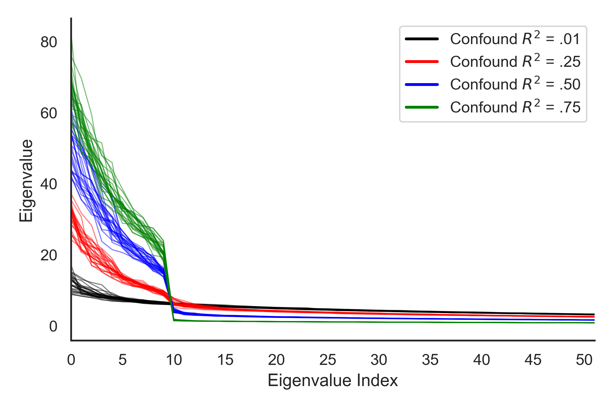
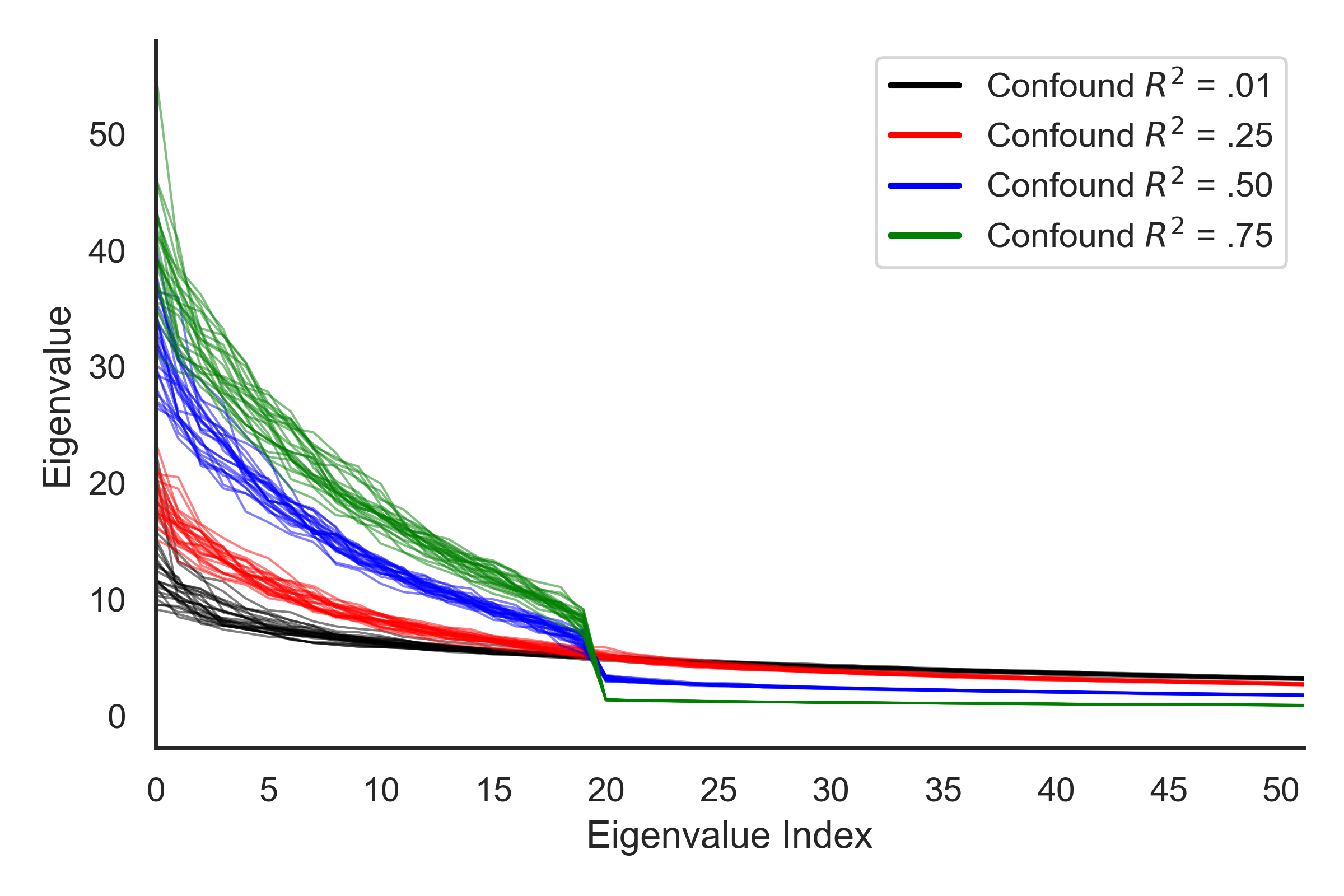
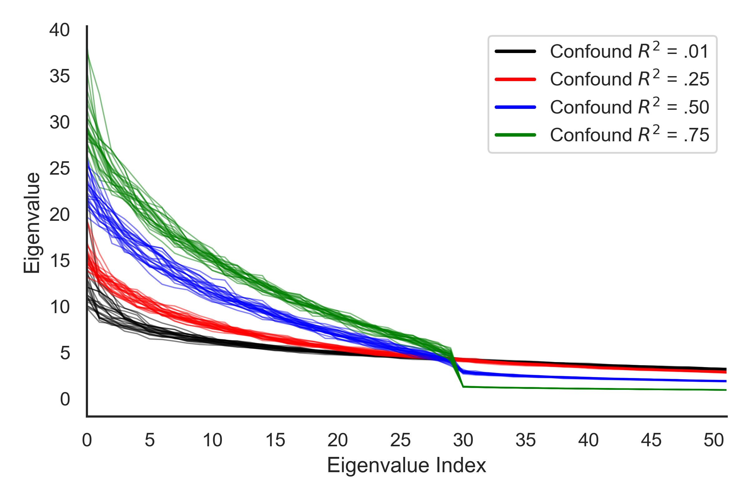
Sensitivity to the number of unobserved confounders. Based on Fig. F.1, the true number of latent factors appears to equal 10, 20, and 30 for $K=5,10$, and 15, respectively. Fig. F.2 illustrates how the results vary for the DeCAMFounder as $K$ increases. In particular, we consider the two tasks described in Section 5: the Wrong Parent Addition Task and the Correct Parent Deletion task. Instead of showing the distribution of the Prop. Times MLL Wrong $>$ MLL True metric across each dataset configuration (e.g., as in Fig. 5), we compute the average of this metric in Fig. F.2 so that we can compare across different choices of $K$. To focus on the effect of $K$ on performance, we set the number of latent factors equal to the correct number of factors. We see that the results in Fig. F.2 do not change significantly relative to the $K=1$ results in Fig. 5. Hence, the performance of the DeCAMFounder appears to be driven by the total variation explained by the confounders (which determine the “spikiness” of the eigenvalues) rather than the number of unobserved confounders.

Figure F.2: Performance sensitivity to the number of unobserved confounders for the DeCAMFounder

# Confounders ($K$)	Confound $R^{2}$	Wrong Parent Addition	Correct Parent Deletion
5	0.01	0.10%	3.90%
	0.25	4.80%	9.50%
	0.50	6.50%	15.50%
	0.75	12.90%	48.00%
10	0.01	0.40%	8.60%
	0.25	2.80%	11.70%
	0.50	3.20%	19.80%
	0.75	4.00%	44.00%
15	0.01	0.60%	0.60%
	0.25	2.70%	6.80%
	0.50	1.30%	24.30%
	0.75	4.00%	46.90%

Figure F.3: Performance sensitivity to the number of latent factors selected for the DeCAMFounder

# Confounders ($K$)	Confound $R^{2}$	Bias Type?	Wrong Parent Addition	Correct Parent Deletion
5	0.01	Under	0.20%	4.70%
		Over	0.10%	3.90%
	0.25	Under	7.60%	7.00%
		Over	3.90%	10.00%
10	0.01	Under	0.40%	7.40%
		Over	0.40%	8.60%
	0.25	Under	2.50%	10.90%
		Over	2.10%	14.20%
15	0.01	Under	1.00%	0.60%
		Over	0.70%	0.60%
	0.25	Under	2.80%	5.10%
		Over	2.80%	5.80%

Sensitivity to the number of latent factors selected. When the confounding strength equals 0.01 and 0.25, estimating the number of latent factors is more challenging since the factors are weaker; see Fig. F.1. In Fig. F.3, we consider two types of biases: underestimating or overestimating the number of latent factors. For underestimation, we set the number of latent factors as 5 fewer than the correct number of latent factors (denoted as “Under”). For overestimation, we set the number of latent factors as 5 more than the correct number of latent factors (denoted as “Over”). The values in Fig. F.3 are similar to those in Fig. F.2, suggesting that the DeCAMFounder is robust to the number of latent factors selected. One reason for this robustness is that when the confounding $R^{2}$ is small (which results in weak latent factors), then the signal strength of the observed variables is larger. Hence, the DAG learning task is easier, allowing for a larger margin of error when estimating the number of latent factors to select in the DeCAMFounder.

Appendix G Additional Figures and Experiments

G.1 Synthetic Data Experiments

In Section 5, we reported on the proportion of times the incorrect parent set was selected over the true parent set. We report on the following additional metric to understand how confidently wrong (or correct) each method is:

1. Log Odds (Wrong vs. True): each score equals the log marginal likelihood (technically an approximation for BIC) of the parent set. Assuming a uniform prior over the set of all parent sets, the log odds (LO) between the wrong and true parent set reduces into the difference between scores:

   $$\begin{split}\text{LO}_{i}&=\log\frac{\mathbb{Q}(X\mid P_{t})\mathbb{Q}(P_{\text{t}})}{\mathbb{Q}(X\mid P_{\text{correct}})\mathbb{Q}(P_{\text{correct}})}\\ &=\text{score}(P_{t})-\text{score}(P_{\text{correct}}).\end{split}$$ (48)

   We report $\max_{1\leq t\in T}\text{LO}_{t}$ for the Wrong Parent Addition task in Fig. G.1 and for the Correct Parent Deletion task in Fig. G.2. A higher value is worse (i.e., it indicates that a method places higher confidence in an incorrect parent set than the true parent set).

(a) Linear SEM

(b) Linear SEM

(c) Non-Linear SEM

(d) Non-Linear SEM

Figure G.1: Results for the Wrong Parent Addition task. 25 total simulations per dataset configuration were performed. See Section 5.1.2 and Section G.1 for a description of the performance metrics.

(a) Linear SEM

(b) Linear SEM

(c) Non-Linear SEM

(d) Non-Linear SEM

Figure G.2: Results for the Correct Parent Deletion task. 25 total simulations per dataset configuration were performed. See Section 5.1.2 and Section G.1 for a description of the performance metrics.

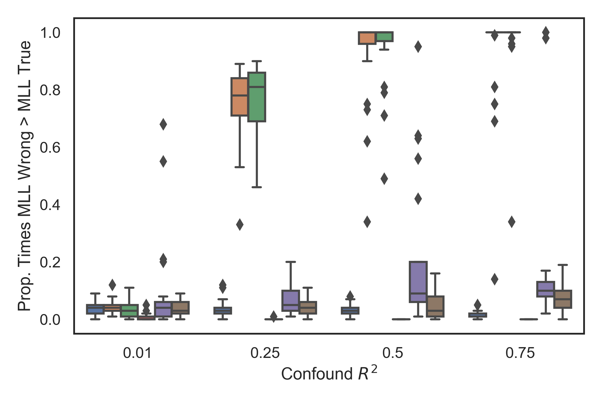
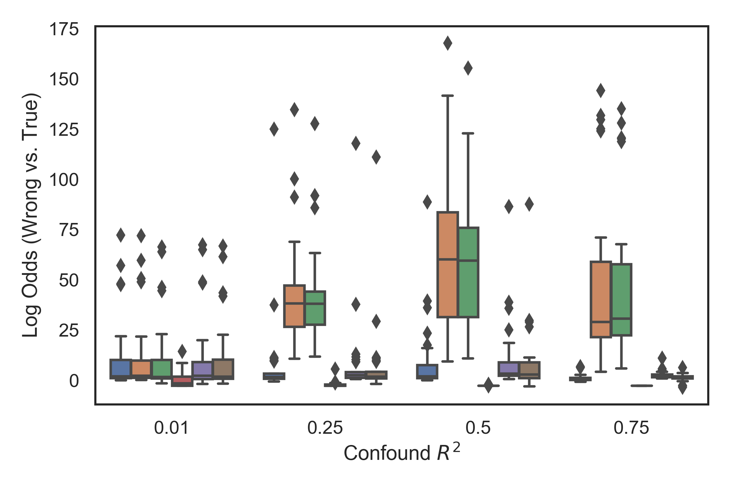
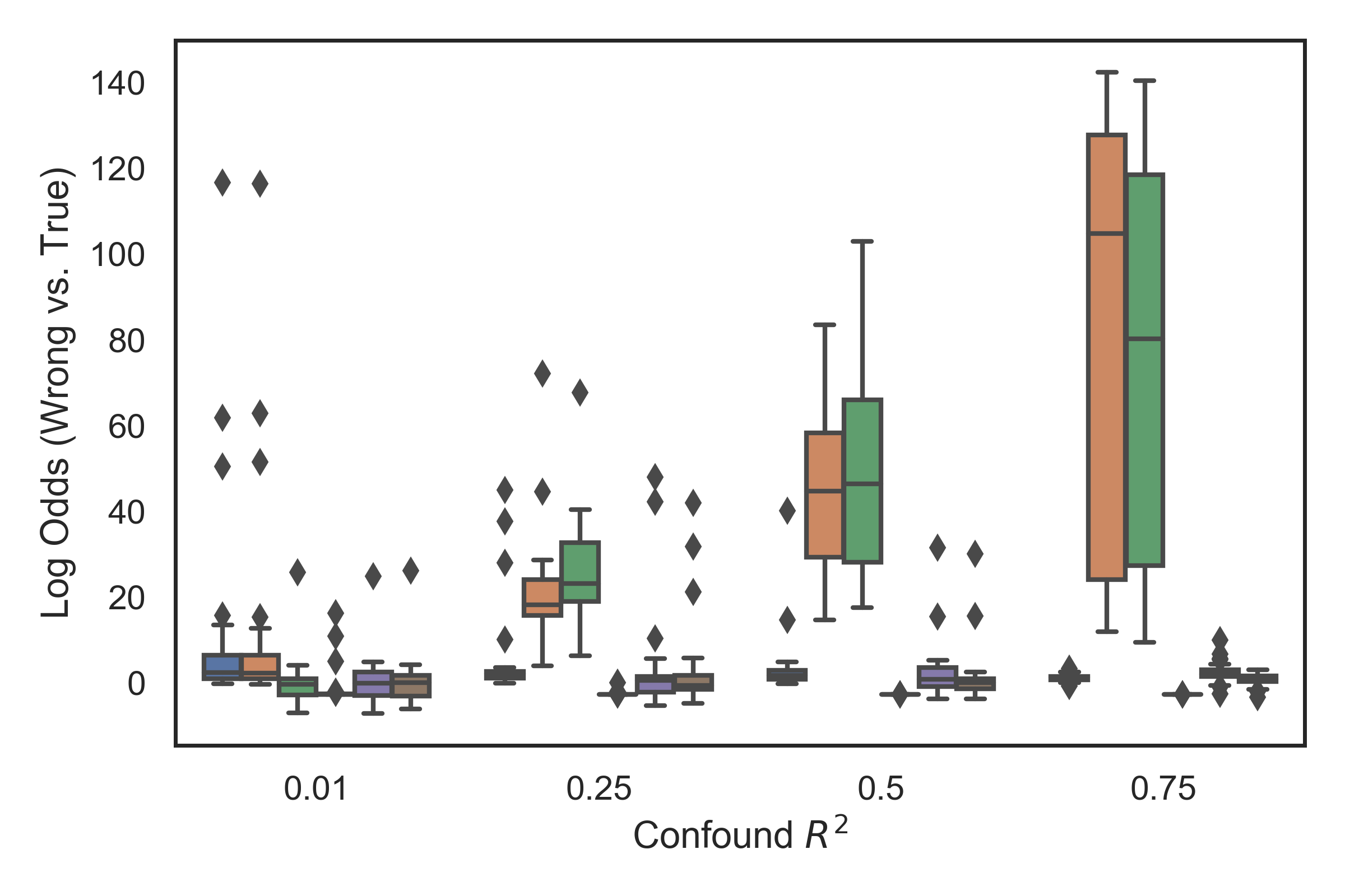
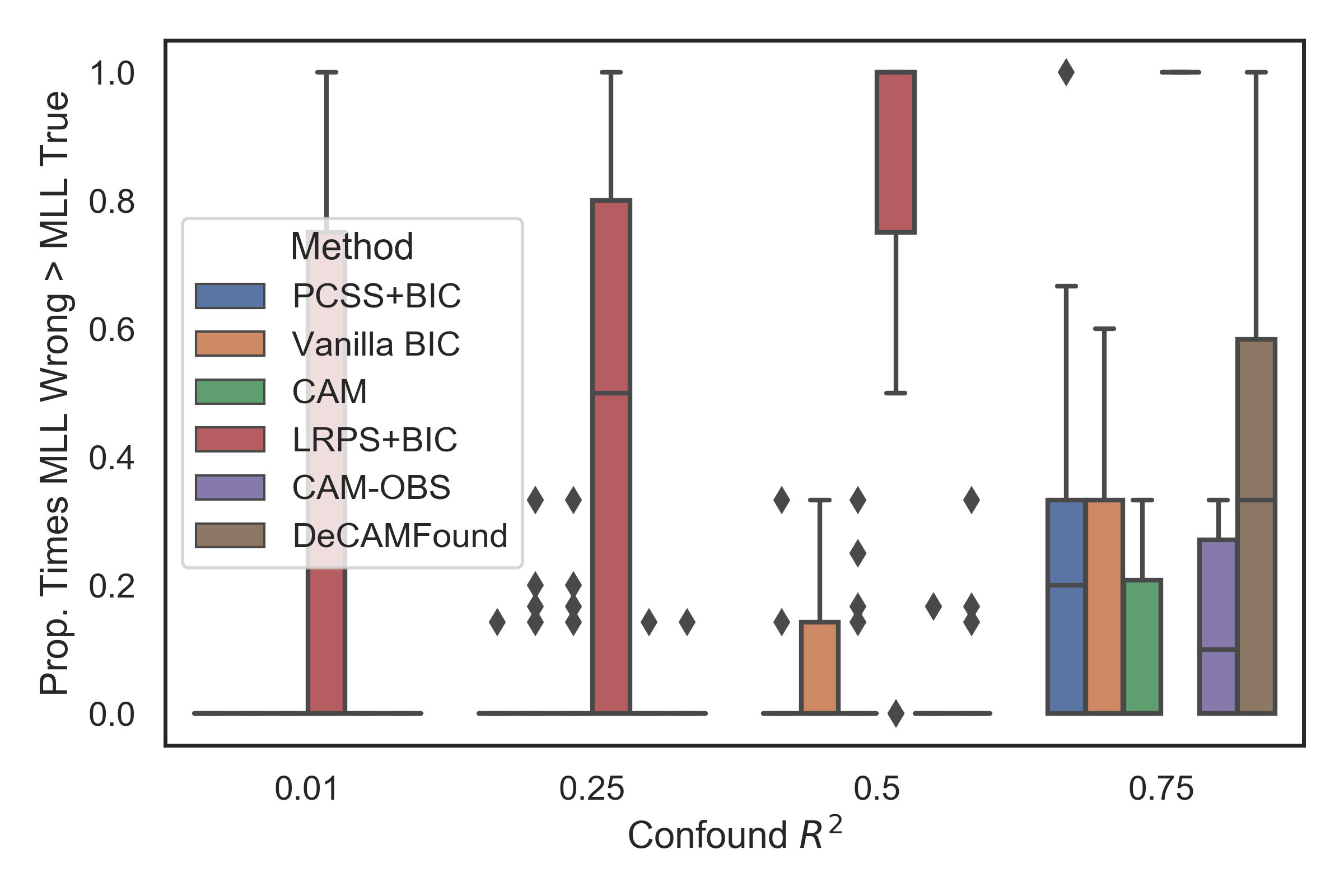
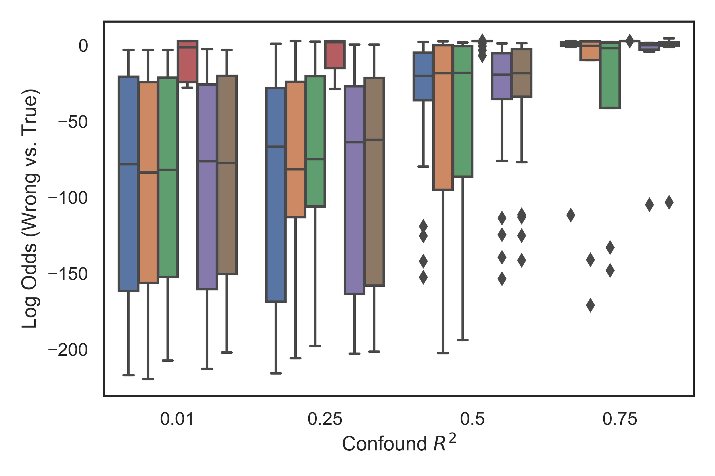
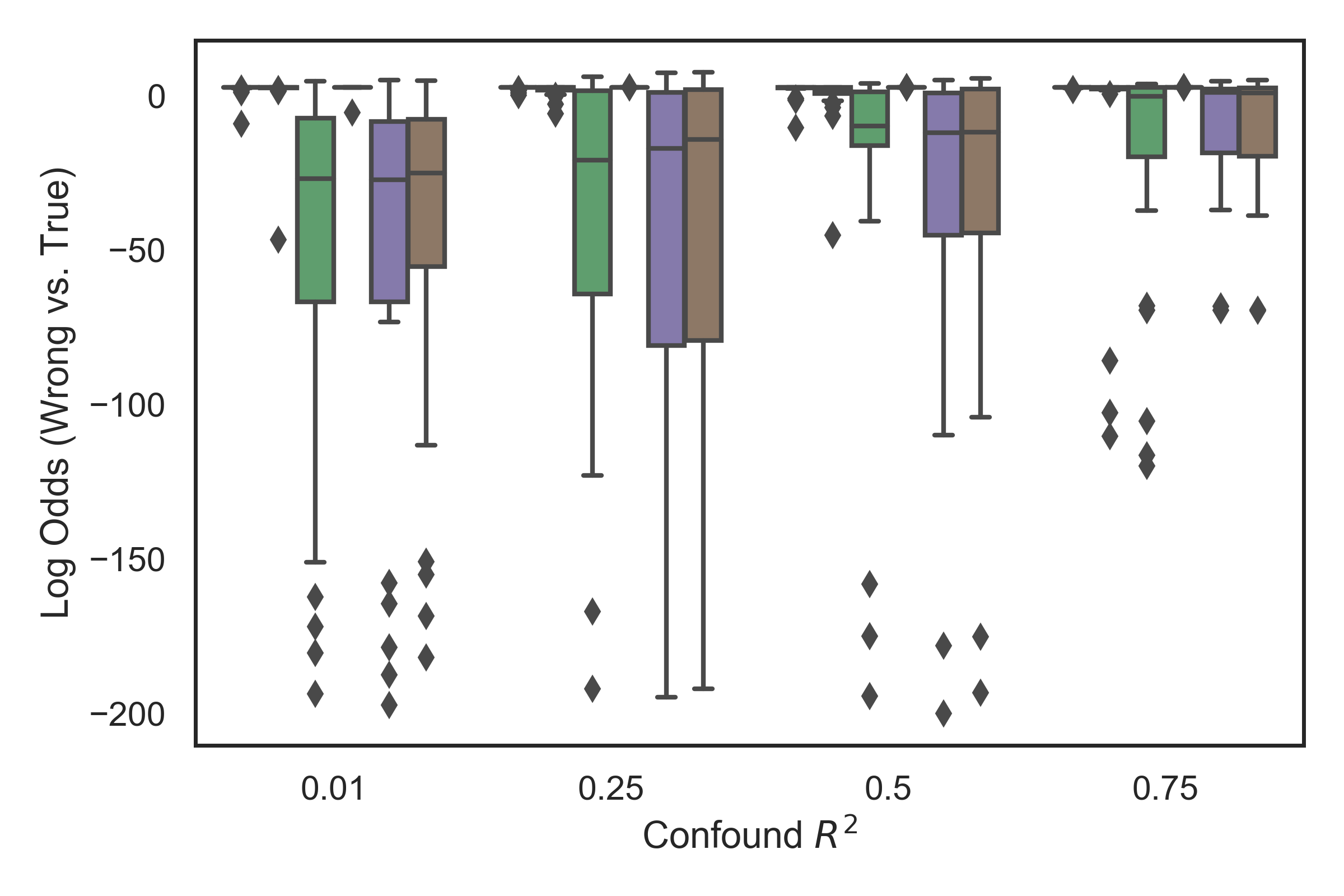
Scoring Candidate DAG Results. We score a candidate set of $T=100$ incorrect DAGs $\mathcal{G}$, built from randomly adding or deleting edges multiple times, starting from the true DAG (i.e., the natural extension of our two parent set evaluation tasks). Since scoring a single graph takes $O(pN^{3})$ for the non-linear methods, we consider fewer settings (i.e., fix the confounding variance to be equal to the signal variance), and only do 10 total simulations instead of 25. These results are shown in Fig. G.3. We report on two metrics:

1. Avg. Posterior SHD: equals $\sum_{t=1}^{T}\text{SHD}(G_{t},\mathcal{G}^{*})\mathbb{Q}(G\mid X)$, where SHD denotes the structural hamming distance to the true graph, and $\mathbb{Q}(G\mid X)$ equals the posterior probability of a graph computed from renormalizing the log marginal likelihood scores. Lower is better.

2. SHD Between MAP and True DAG: reports the SHD from the true DAG for the highest scoring graph (i.e., the maximum a posteriori estimate). Lower is better.

Fig. G.3 shows that linear methods, even if they account for confounding, suffer in the non-linear setting. This advantage of modeling non-linearities agrees with the results, for example, in Bühlmann et al. (2014). Fig. G.3 also shows that, as in the Correct Parent Deletion Task, LRPS suffers even in the linear setting because the induced undirected graph is very sparse (and hence often favors deleting true edges). Finally, Fig. G.3 shows that both CAM-OBS (trivially) and our method are robust to both non-linearities and confounding.

(a) SHD

(b) Average SHD

Figure G.3: Results for the candidate DAG scoring task. 10 total simulations per dataset configuration (i.e., linear / non-linear) were performed.

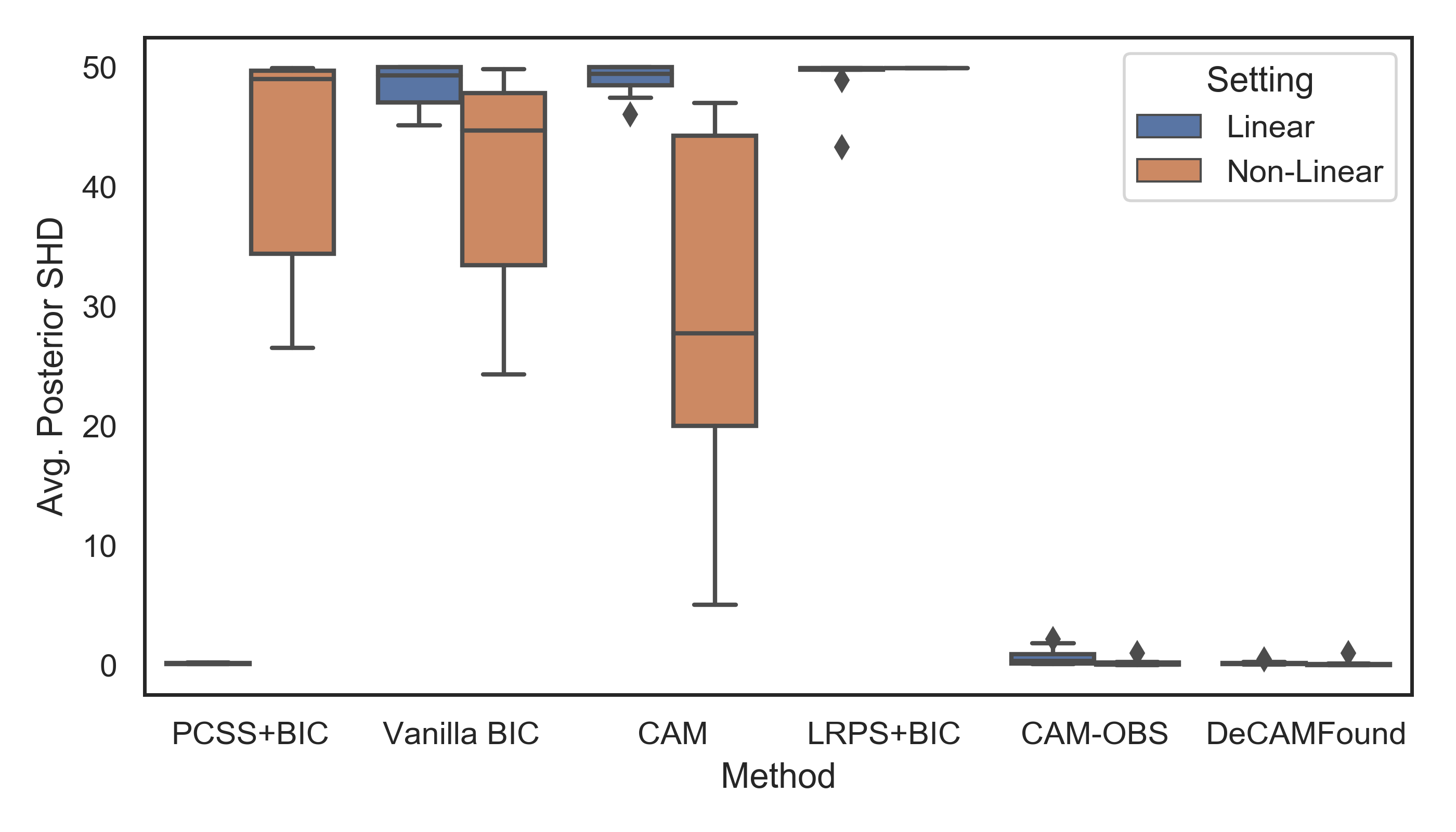
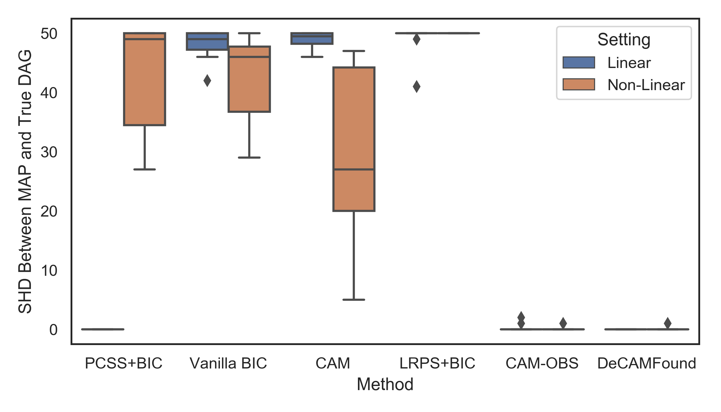
G.2 Ovarian Cancer Dataset

Scree Plot. Analyzing the spectrum of the data matrix consisting of the 486 observed genes in Fig. G.4 shows that there are about 7 spiked eigenvalues.

Pervasive TF Gene Correlations. 7/15 TFs have edges with more than 75 genes according to NetBox (i.e., these TFs might play the role of pervasive confounders). We summarize the absolute value of the correlations between these 7 TFs and the 486 genes in Fig. G.5.

Removing the Effect of a Latent TF via PCSS. See Fig. G.7.

Figure G.4: PCA scree plot when the input data matrix consists of the 486 observed genes. Based on this scree plot, we select $K=7$ components for the spectral methods.

Figure G.5: Absolute value of correlations between TFs and the 486 observed genes. Only TFs with at least 75 edges are shown.

Figure G.6: Out of the 15 latent TFs, BIRC3 has the highest absolute correlation with NFKB1 and the smallest absolue correlation with JUN. BIRC3-pcss refers to the total latent confounding variation estimated for that gene via PCSS. BIRC3 refers to the actual observed values of the gene. BIRC3-pcss is correlated with NFKB1 (which is correlated with BIRC3) and not correlated with JUN.

Figure G.7: Top left: scatterplot of two genes that are conditionally independent given each parents’ gene neighborhood sets and TFs but dependent when removing the TFs. Top right: scatter plot of each gene for the TF that has the highest correlation with both genes. Bottom left: correlation with the transcription factor after removing the estimated confounder sufficient statistics from each gene. Bottom right: weaker correlation after removing the confounder sufficient statistics from each gene. Since both genes are still marginally dependent given the TFs without conditioning on the parent sets, the genes are still correlated in the bottom right figure.

References

- Bernstein et al. (2020) Bernstein, D., Saeed, B., Squires, C. and Uhler, C. (2020) Ordering-based causal structure learning in the presence of latent variables. Proceedings of Machine Learning Research, 108, 4098–4108.
- Bühlmann et al. (2014) Bühlmann, P., Peters, J. and Ernest, J. (2014) CAM: Causal additive models, high-dimensional order search and penalized regression. Annals of Statistics, 42, 2526–2556.
- Cerami et al. (2010) Cerami, E., Demir, E., Schultz, N., Taylor, B. S. and Sander, C. (2010) Automated network analysis identifies core pathways in glioblastoma. PLOS ONE, 5, 1–10.
- Chandrasekaran et al. (2012) Chandrasekaran, V., Parrilo, P. A. and Willsky, A. S. (2012) Latent variable graphical model selection via convex optimization. Annals of Statistics, 40, 1935–1967.
- Chandrasekaran et al. (2009) Chandrasekaran, V., Sanghavi, S., Parrilo, P. A. and Willsky, A. S. (2009) Sparse and low-rank matrix decompositions. In 2009 47th Annual Allerton Conference on Communication, Control, and Computing (Allerton), 962–967.
- Chickering (2002) Chickering, D. M. (2002) Optimal structure identification with greedy search. Journal of Machine Learning Research, 3, 507–554.
- Colombo et al. (2012) Colombo, D., Maathuis, M. H., Kalisch, M. and Richardson, T. S. (2012) Learning high-dimensional directed acyclic graphs with latent and selection variables. Annals of Statistics, 40, 294–321.
- Evans (2016) Evans, R. (2016) Graphs for margins of Bayesian networks. Scandinavian Journal of Statistics, 43, 625–648.
- Fan et al. (2013) Fan, J., Liao, Y. and Mincheva, M. (2013) Large covariance estimation by thresholding principal orthogonal complements. Journal of the Royal Statistical Society Series B, 75, 603–680.
- Friedman et al. (2000) Friedman, N., Linial, M., Nachman, I. and Pe’er, D. (2000) Using Bayesian networks to analyze expression data. In Proceedings of the Fourth Annual International Conference on Computational Molecular Biology, 127–135.
- Friedman and Nachman (2000) Friedman, N. and Nachman, I. (2000) Gaussian process networks. In Proceedings of the 16th Conference on Uncertainty in Artificial Intelligence, 211–219.
- Frot et al. (2019) Frot, B., Nandy, P. and Maathuis, M. H. (2019) Robust causal structure learning with some hidden variables. Journal of the Royal Statistical Society: Series B, 81, 459–487.
- Gardner et al. (2018) Gardner, J., Pleiss, G., Weinberger, K. Q., Bindel, D. and Wilson, A. G. (2018) GPyTorch: Blackbox matrix-matrix Gaussian process inference with GPU acceleration. In Advances in Neural Information Processing Systems.
- Van de Geer et al. (2000) Van de Geer, S., Gill, R., Ripley, B., Ross, S., Silverman, B., Williams, D. and Stein, M. (2000) Empirical Processes in M-Estimation. Cambridge Series in Statistical and Probabilistic Mathematics.
- Gyorfi et al. (2003) Gyorfi, L., Kohler, M., Krzyzak, A. K. and Walk, H. (2003) A distribution-free theory of nonparametric regression. Journal of the American Statistical Association, 98, 1084–1084.
- Harrington and Annunziata (2019) Harrington, B. S. and Annunziata, C. M. (2019) NF-kB signaling in ovarian cancer. Cancers (Basel), 8.
- Haughton (1988) Haughton, D. M. A. (1988) On the Choice of a Model to Fit Data from an Exponential Family. The Annals of Statistics, 16.
- Hoyer et al. (2009) Hoyer, P., Janzing, D., Mooij, J. M., Peters, J. and Schölkopf, B. (2009) Nonlinear causal discovery with additive noise models. In Advances in Neural Information Processing Systems, vol. 21.
- Kalisch and Bühlmann (2007) Kalisch, M. and Bühlmann, P. (2007) Estimating high-dimensional directed acyclic graphs with the PC-algorithm. Journal of Machine Learning Research, 8, 613–636.
- Koller and Friedman (2009) Koller, D. and Friedman, N. (2009) Probabilistic graphical models: principles and techniques. MIT press.
- Kusner et al. (2017) Kusner, M. J., Loftus, J., Russell, C. and Silva, R. (2017) Counterfactual fairness. In Advances in Neural Information Processing Systems, vol. 30.
- Mooij et al. (2009) Mooij, J. M., Janzing, D., Peters, J. and Schölkopf, B. (2009) Regression by dependence minimization and its application to causal inference in additive noise models. In Proceedings of the 26th Annual International Conference on Machine Learning, ICML 2009, Montreal, Quebec, Canada, June 14-18, 2009, vol. 382, 745–752.
- Mooij et al. (2016) Mooij, J. M., Peters, J., Janzing, D., Zscheischler, J. and Schölkopf, B. (2016) Distinguishing cause from effect using observational data: Methods and benchmarks. Journal of Machine Learning Research, 17, 1–102.
- Pearl (2009) Pearl, J. (2009) Causality: Models, Reasoning and Inference. Cambridge University Press, 2nd edn.
- Peters et al. (2014) Peters, J., Mooij, J. M., Janzing, D. and Schölkopf, B. (2014) Causal discovery with continuous additive noise models. Journal of Machine Learning Research, 15, 2009–2053.
- Rasmussen and Williams (2006) Rasmussen, C. E. and Williams, C. K. I. (2006) Gaussian Processes for Machine Learning. The MIT Press.
- Richardson and Spirtes (2002) Richardson, T. and Spirtes, P. (2002) Ancestral graph Markov models. Annals of Statistics, 30, 962–1030.
- Robins et al. (2000) Robins, J., Hernan, M. A. and Brumback, B. (2000) Marginal structural models and causal inference in epidemiology. Epidemiology, 11, 550–60.
- Rudin (1974) Rudin, W. (1974) Functional Analysis. International series in pure and applied mathematics. Tata McGraw-Hill.
- Shah et al. (2020) Shah, R. D., Frot, B., Thanei, G.-A. and Meinshausen, N. (2020) Right singular vector projection graphs: fast high dimensional covariance matrix estimation under latent confounding. Journal of the Royal Statistical Society: Series B (Statistical Methodology), 82, 361–389.
- Solus et al. (2020) Solus, L., Wang, Y., Matejovicova, L. and Uhler, C. (2020) Consistency guarantees for permutation-based causal inference algorithms. Biometrika.
- Spirtes et al. (2000) Spirtes, P., Glymour, C. and Scheines, R. (2000) Causation, Prediction, and Search. The MIT Press, 2nd edn.
- Wainwright (2019) Wainwright, M. J. (2019) High-Dimensional Statistics: A Non-Asymptotic Viewpoint. Cambridge University Press.
- Wang and Fan (2017) Wang, W. and Fan, J. (2017) Asymptotics of empirical eigenstructure for high dimensional spiked covariance. Annals of Statistics, 45, 1342–1374.
- Wang and Blei (2019) Wang, Y. and Blei, D. M. (2019) The blessings of multiple causes. Journal of the American Statistical Association, 114, 1574–1596.