Training Larger Networks for Deep Reinforcement Learning
Abstract
The success of deep learning in the computer vision and natural language processing communities can be attributed to training of very deep neural networks with millions or billions of parameters which can then be trained with massive amounts of data. However, similar trend has largely eluded training of deep reinforcement learning (RL) algorithms where larger networks do not lead to performance improvement. Previous work has shown that this is mostly due to instability during training of deep RL agents when using larger networks. In this paper, we make an attempt to understand and address training of larger networks for deep RL. We first show that naively increasing network capacity does not improve performance. Then, we propose a novel method that consists of 1) wider networks with DenseNet connection, 2) decoupling representation learning from training of RL, 3) a distributed training method to mitigate overfitting problems. Using this three-fold technique, we show that we can train very large networks that result in significant performance gains. We present several ablation studies to demonstrate the efficacy of the proposed method and some intuitive understanding of the reasons for performance gain. We show that our proposed method outperforms other baseline algorithms on several challenging locomotion tasks.
1 Introduction
We have witnessed huge improvements in the fields of computer vision (CV) and natural language processing (NLP) in the last decade (Krizhevsky et al., 2012; He et al., 2016; Huang et al., 2017; Devlin et al., 2019; Brown et al., 2020). These developments could largely be attributed to training of very large neural networks with millions (or even billions or trillions) of parameters which can be trained using massive amounts of data and an appropriate optimization technique to stabilize training. In general, the motivation of training larger networks comes from the intuition that larger networks allow better solutions as they increase the search space of possible solutions. Having said that, neural network training largely relies on the ability to find good minimizers of highly non-convex loss functions. These loss functions are also governed by the choices of network architecture, batch size, etc. This has also driven a lot of research in these communities towards understanding the underlying reasoning for performance gains (Lu et al., 2017; Zhang et al., 2017; Nguyen & Hein, 2017; Li et al., 2018).

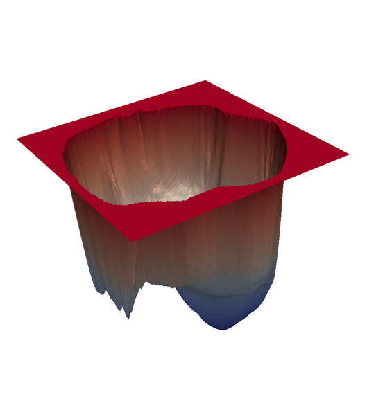
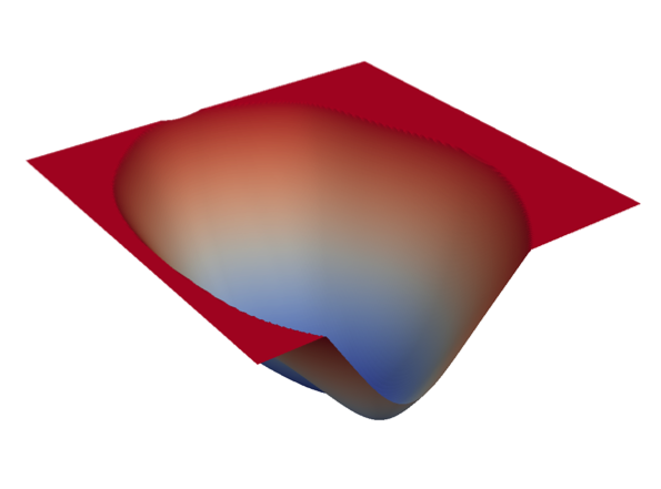
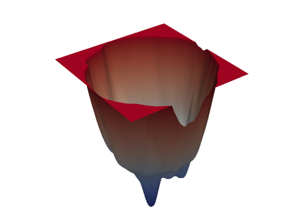
In a striking contrast, Deep Reinforcement Learning (DRL) community has not reported similar trend with regards to training larger networks for RL. It has been reported in some studies that deep RL agents experience instability while training with larger networks (Henderson et al., 2018; van Hasselt et al., 2018; Achiam et al., 2019; Sinha et al., 2020). As an example, in Fig. 1, we show the results of an Soft Actor Critic (SAC) (Haarnoja et al., 2018) agent that uses Multi-layered Perceptron (MLP) for function approximation with increasing number of layers while fixing its unit size to 256 (also notice the loss surface). These plots show that using deeper networks naively leads to poor performance for a deep RL agent. Consequently, using larger networks for training deep RL networks is not fully understood, and thus is limiting in several ways. As a result, most of the reported work in literature end up using similar hyperparameters (i.e., network structure, number and size of layers, etc.). Our work is motivated by this limitation, and we make an attempt to explore the interplay between the size, structure, training and performance of deep RL agents to provide some intuition and guidelines for using larger networks.
In light of these facts, we present a large-scale study and provide empirical evidence for using larger networks for training DRL agents. We first highlight the challenges that one might come across while using larger networks for training deep RL agents. To circumvent these problems, we integrate a three-fold approach: decoupling feature representation from RL to efficiently produces high dimensional features, employing DenseNet architecture to propagate richer information, and using distributed training methods to collect more on-policy transitions to reduce overfitting. Our method is a novel architecture that combines these three elements, and we demonstrate our proposed method significantly improves the performance of RL agents in continuous control tasks. We also conduct an ablation study to show what component contributes the performance gain. Our contributions can be summarized as follows:
-
•
We conduct a large scale study on employing larger networks for DRL agents, and empirically show that, in contrary to deeper networks, wider networks can improve performance.
-
•
We propose a novel network architecture that synergistically combines recently proposed techniques to stabilize the training: decoupling representation learning from RL, DenseNet architecture, and distributed training, to demonstrate it significantly improves performance.
-
•
We analyze the performance gain of our method using metrics of effective ranks of features as well as visualization of loss function landscape of RL agents.

2 Related Work
Our work is broadly motivated by (Henderson et al., 2018) that empirically demonstrates DRL algorithms are vulnerable to different training choices like architectures, hyperparameters, activation functions, etc. The paper compares performance on different number of units and layers, and demonstrates larger networks do not consistently improve performance. This is contrary to our intuition considering the recent progress on solving computer vision tasks such as ImageNet (Deng et al., 2009): larger and more complex network architectures have proven to achieve better performance (Krizhevsky et al., 2012; He et al., 2016; Huang et al., 2017; Tan & Le, 2019).
Sutton & Barto (2018) identifies a deadly triad of function approximation, bootstrapping, and off-policy learning. When these three properties are combined, learning can be unstable, and potentially diverge with the value estimates becoming unbounded. Some prior works have challenged to mitigate this problem, including target networks (Mnih et al., 2015), double Q-learning (Van Hasselt et al., 2016), n-step learning (Hessel et al., 2018), etc. Our challenge of training larger networks is specifically related to function approximation, however, as the deadly triad is entangled in a complex manner, we also have to deal with the other problems. As for the network size, some studies investigate the effect of making network larger for continuous control task using MLP (Fu et al., 2019; Achiam et al., 2019) and Atari games using CNN (van Hasselt et al., 2018), and concluded the larger networks tend to perform better, but also become unstable and prone to diverge more. Andrychowicz et al. (2021) and Liu et al. (2021) performed similar study on on-policy methods and showed too small or large networks can cause significant drop in performance of the policy. While these studies are limited to relatively small size (hundreds of units with several layers), we will have more thorough study on much larger networks, combination of state representation learning, and employing different network architectures.
To build a large network, unsupervised learning has been used to learn powerful representations for downstream tasks in natural language processing (Devlin et al., 2019; Radford et al., 2019) and computer vision (He et al., 2020; Chen et al., 2020). In the context of RL, auxiliary tasks such as predicting the next state conditioned on the past state(s) and action(s) have been widely studied to improve the sample efficiency of the RL algorithms (Jaderberg et al., 2017; Shelhamer et al., 2017; Ha & Schmidhuber, 2018). For the state-input setting, researchers have generally focused on learning a good representation that produces low dimensional features (Munk et al., 2016; Lesort et al., 2018). Contrary to that, Ota et al. (2020) proposes the use of online feature extractor network (OFENet) that intentionally increases input dimensionality, and demonstrates that larger feature size enables to improve RL performance on both sample efficiency and control performance. We leverage this idea and use larger input (or feature) for RL agents as well as using larger networks for the policy and the value function networks.
3 Method
While recent studies suggest that larger networks for DRL agents have potential to improve performance, it is non-trivial to alleviate some potential issues that lead to instability when using larger networks to train RL agents.
Our method is based on two main key ideas: allowing better feature propagation using good network architectures and using huge amounts of more on-policy data using distributed training to avoid overfitting in larger networks. We first obtain good features apart from RL using an auxiliary task, and then propagate the features more efficiently by employing the DenseNet (Huang et al., 2017) architecture. Also, we use a distributed RL framework that can mitigate the potential overfitting problem. In the following, we describe in detail the three elements we use for training larger networks for deep RL agents. Our proposed approach is shown as a schematic in Fig. 2.
3.1 Decoupling Representation Learning from RL
While the simplicity of learning whole networks in an end-to-end fashion is appealing, updating all parameters of a large network using just a scalar reward signal can result in very inefficient training (Stooke et al., 2020). Decoupling unsupervised pretraining from downstream tasks is common in computer vision (He et al., 2020; Henaff, 2020). Taking inspiration from this, we adopt the online feature extractor network (OFENet) (Ota et al., 2020) to learn meaningful features separately from training of RL.
OFENet learns representation vectors of states and state-action pairs , and provides them to the agent instead of original inputs and , which gives significant performance improvements on continuous robot control tasks. As the representation vectors and are designed to have much higher dimensionality than original inputs, OFENet matches our philosophy of providing larger solution space that allows us to find better policy. The representations can be obtained by learning the mappings and , which have parameters by using an auxiliary task of predicting the next state from the current state and action representation as:
| (1) |
where is represented as a linear combination of the representation . The learning of the auxiliary task is done concurrently with the learning of the downstream RL task. In our experiments, we allow input dimensionality much bigger than previously presented in (Ota et al., 2020). Furthermore, we also increase the network size of RL agents (see A.2 for the number of network parameters used in our experiments). For more details, interested readers are referred to (Ota et al., 2020).
3.2 Distributed Training
In general, larger networks need more data to improve accuracy of function approximation (Deng et al., 2009; Hernandez et al., 2021) and mitigate overfitting problem (Bishop, 2006). MLP with a large number of hidden layers is in particular known to cause an over-fitting to training data, which often results in inferior performance to shallow networks (Bengio et al., 2007; Ramchoun et al., 2017). In the context of RL, while we are training and evaluating on the same environment, there is still problem of overfitting: the agent is only trained on limited trajectories it has experienced, which cannot cover the whole state-action space of the environment (Liu et al., 2021). Fu et al. (2019) showed overfitting to the experience replay exists, and Fedus et al. (2020) empirically showed having more on-policy data in replay buffer, i.e. collecting more than one transition while updating policy one time can improve performance of RL agent.
In light of these studies, we employ distributed RL framework, which leverages distributed training architectures that decouples learning from collecting transitions by utilizing many actors running in parallel on separate environment instances (Horgan et al., 2018; Kapturowski et al., 2019). In particular, we use Ape-X (Horgan et al., 2018) framework, where a single learner receives experiences from distributed prioritized replay (Schaul et al., 2016), and multiple actors collect transitions in parallel (see Fig. 2). This helps increase the number of data that are close to the current policy, i.e. more on-policy data, which can improve performance of off-policy RL agents (Fedus et al., 2020) and mitigate rank collapse issues of Q-networks (Aviral Kumar & Levine, 2021). One difference is that we do not use the RL algorithm used in (Horgan et al., 2018), but instead use standard off-policy RL algorithms: SAC (Haarnoja et al., 2018) and Twin Delayed Deep Deterministic policy gradient algorithm (TD3) (Fujimoto et al., 2018) in our experiments.
3.3 Network Architectures
Tremendous developments have been made in the computer vision community in designing sophisticated architectures that enable training of very large networks (He et al., 2016; Huang et al., 2017; Tan & Le, 2019). Huang et al. (2017) proposed Dense Convolutional Network (DenseNet) that has a skip connection that directly connects each layer to all subsequent layers as: , where is the output of the layer, thus all the inputs are concatenated into a single tensor. Here, is a composite function which consists of a sequence of convolutions, Batch Normalization (BN) (Ioffe & Szegedy, 2015), and an activation function. An advantage of DenseNet is its improved flow of information and gradients throughout the network, which makes the large networks easier to train. We borrow this architecture to train large networks for RL agents.
Although using DenseNet architecture for DRL agents is existing, it has not been fully explored yet. D2RL (Sinha et al., 2020) employs a modified DenseNet architecture which concatenates the state or the state-action pair to each hidden layer of the MLP networks except the last linear layer. Contrary to this modified version, Ota et al. (2020) exactly follows the original DenseNet: it uses the dense connection that concatenates all the outputs of the previous layer instead of only the state or the state-action pair for training only OFENet, and is not used for training RL agents. We also follow the original DenseNet architecture as done in (Ota et al., 2020) to represent the policy and the value function networks. The schematic of the DenseNet architecture is also shown in Fig. 2. We omit BN for SAC agent because we found it inhibits improving performance.
4 Experiments
In this section, we present results of numerical experiments in order to answer some relevant underlying questions posed in this paper. In particular, we answer the following questions.
-
•
Can RL agents benefit from usage of larger networks during training? More concretely, can using larger networks lead to better policies for DRL agents?
-
•
What characterizes a good architecture which facilitates better performance when using larger networks?
-
•
Can our method work across different RL algorithms as well as different tasks?
Experimental settings
We run all each experiment independently with five seeds, and the average and standard deviation results will be reported, which are solid lines and shaded regions when we show training curves. The horizontal axis of a training curve is the number of gradient steps, which is not identical to the number of steps an agent interacts with an environment only when we use the distributed replay. The network architectures, optimizers, and hyperparameters are the same as used in their original papers (Haarnoja et al., 2018; Fujimoto et al., 2018; Ota et al., 2020) unless otherwise noted. We used single NVIDIA Tesla V100 GPU with Xeon Gold 6148 Processor. Appendix A shows more details of experimental settings.
Evaluation metrics
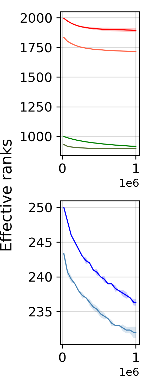
We evaluate the experimental results on two metrics: average return and the recently proposed effective ranks (Aviral Kumar & Levine, 2021) of the features matrices of Q-networks. Aviral Kumar & Levine (2021) showed that MLPs used for approximating policy and value functions that use bootstrapping leads to reduction in the effective rank of the feature, and this rank collapse for the feature matrix results in poorer performance. We will show the effective rank of the features in the penultimate layer of the Q-networks to evaluate whether our proposed architecture can alleviate the rank collapse issue.
4.1 Does increasing the size of networks fail to improve performance?
In the first set of experiments, we try to investigate if increasing network size always leads to poor performance. We quantitatively measure the effectiveness of increasing the network size by changing the number of units and layers while the other parameters are fixed.
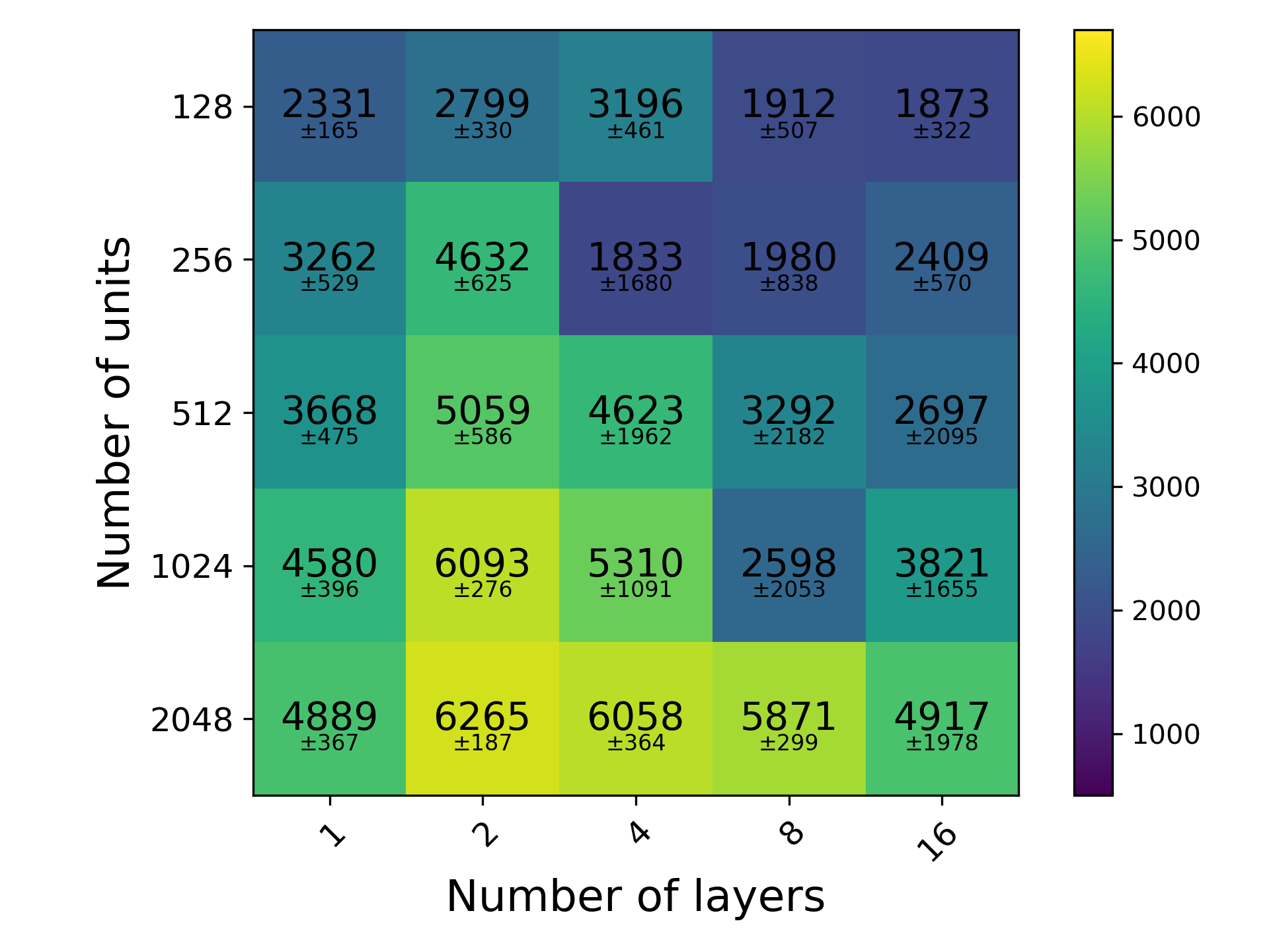
Figure 1 shows the training curves when increasing the number of layers while the unit size is fixed to . As we described in Sec. 1, we observe that the performance becomes worse as the network becomes deeper. In Fig. 4, we show the effect of increasing the number of units while the number of layers is fixed to . Contrary to the results when making the network deeper, we can observe consistent improvement when making the network wider. In order to investigate more thoroughly, we also conduct a grid search, where we sample each parameter of the network from , and and evaluate the performance in Fig. 4. We can see the monotonic improvement in performance when widening networks on almost all depth of the network.
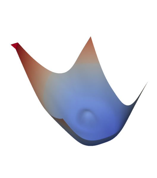
This result is in line with the general belief that training deeper networks is, in general, harder and is more susceptible to choice of hyperparameters (Bengio et al., 2007; Ramchoun et al., 2017). This could be attributed to vanishing gradient problem with increasing number of layers (Bengio et al., 1994). However, we found that the reason that deeper networks are harder to train than wider network cannot be attributed to vanishing gradient, rather it results from the sharpness of the loss surface curvatures (Li et al., 2018). We show the loss surface of the deeper network () in Fig. 1 and the wider network () in Fig. 4 by using the visualization method proposed in (Li et al., 2018) with the loss of TD error of Q-functions of SAC agents (see Appendix A.3 for more details). These figures show that wider networks have nearly convex surface while deeper networks have more complex loss surface which could be susceptible to choice of hyperparameters (Li et al., 2018). Comparison of deeper and wider networks have also been done in several works (Wu et al., 2019; Nguyen & Hein, 2017; Li et al., 2018), where wider networks are prone to have more generalization capability due to their smooth loss functions.
From these results, we observe and conclude that larger networks can be effective in improving deep RL performance. In particular, we achieve consistent performance gains when widening individual layers instead of going deeper. Consequently, we fix the number of layers to , and only change the number of units to learn larger networks in the following experiments.

4.2 Architecture Comparison
In the next set of experiments, we try to investigate the role of synergistic combination of connectivity architecture, state-representation and distributed training in allowing usage of larger networks for training deep RL agents. A brief introduction to these techniques is described in Sec. 3.
Connectivity architecture
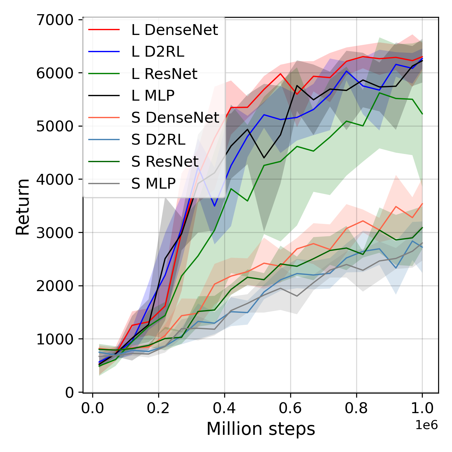
We first compare four connectivity architectures: standard MLP, MLP-ResNet, MLP-DenseNet, and MLP-D2RL, which is a recently proposed architecture to improve RL performance. MLP-ResNet is a modified version of Residual Networks (ResNet) (He et al., 2016, 2016), which has a skip-connection that bypasses the non-linear transformations with an identity function: , where is the output of the layer, and is a residual module, which consists of fully connected layer and nonlinear activation function. An advantage of this architecture is that the gradient can flow directly through the identity mapping from top layers to bottom layers. MLP-D2RL is identical to (Sinha et al., 2020), and MLP-DenseNet is our proposed architecture that is defined in Sec. 3.3. We compare these four architectures on both small network (, denoted by S) and large networks (, denoted by L).
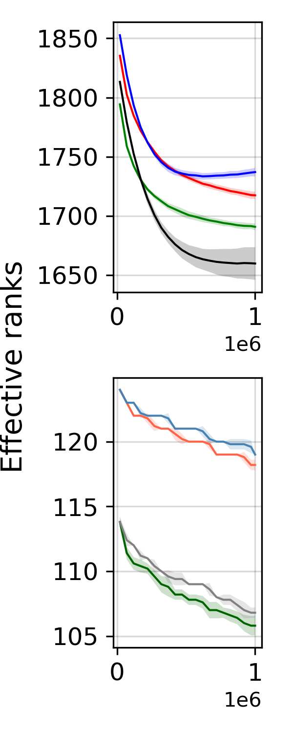
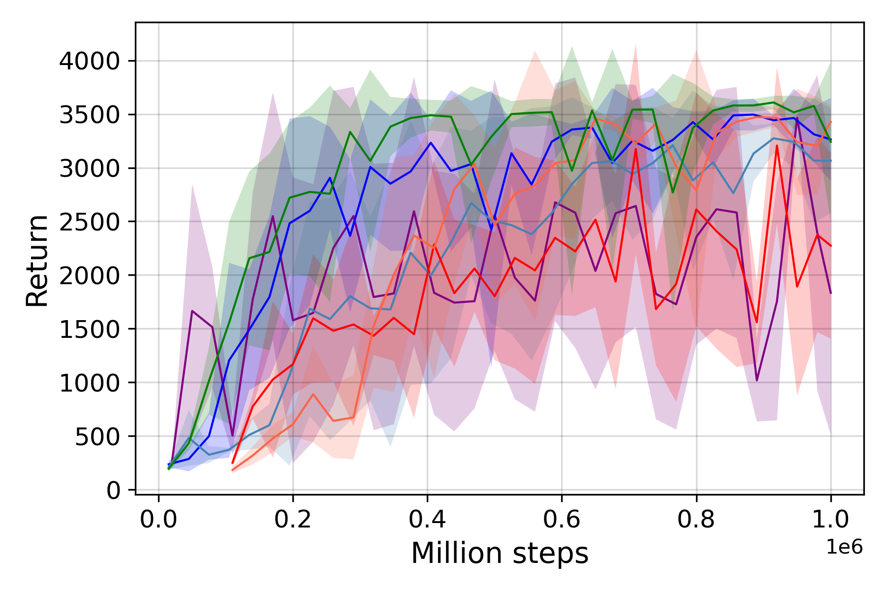
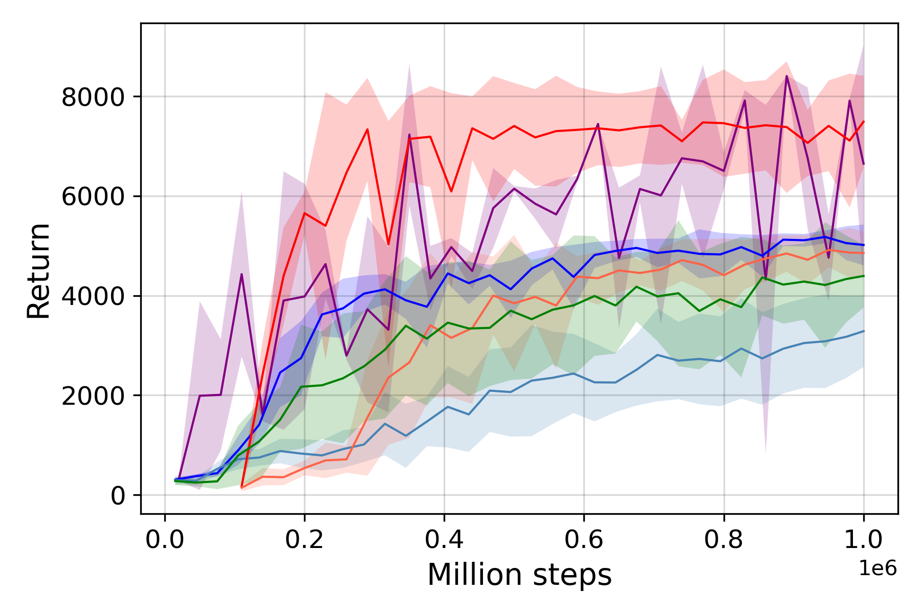
Figure 5 shows the training curves of average return in Fig. 5, and the effective ranks in Fig. 5. The results show that our MLP-DenseNet achieves the highest return on both small and large networks, while mitigating rank collapse comparable to MLP-D2RL. This shows that the MLP-DenseNet is the best architecture among these four choices, and thus we employ this architecture for both the policy and the value function network in the following experiments.
Decoupling representation learning from RL
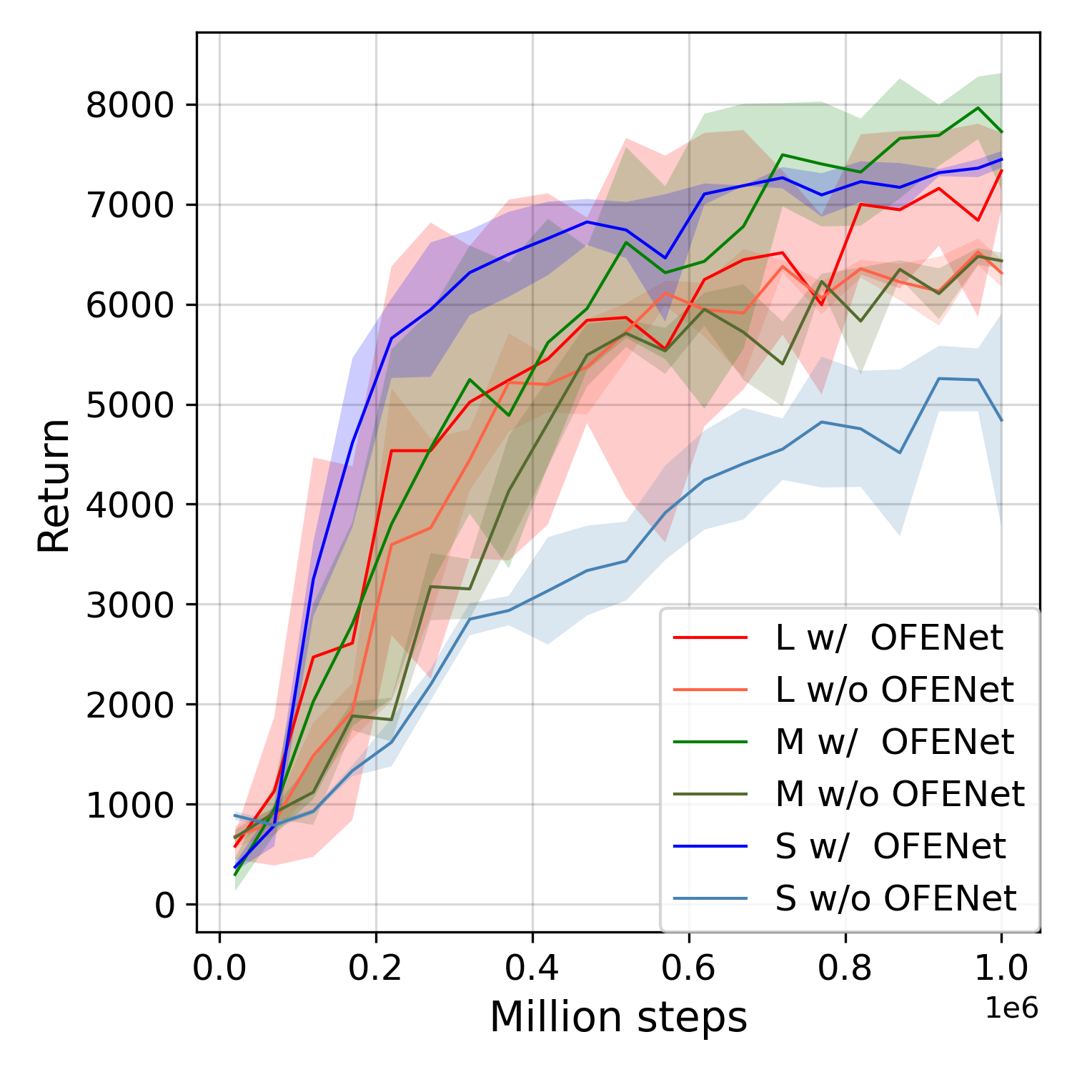
Next, we evaluate the effectiveness of using OFENet (see Sec. 3.1) to decouple representation learning from RL. In order to evaluate the performance on different network size, we sample the number of units from , which we respectively denote S, M, and L, and compare these against the baseline SAC agents, which do not use OFENet and are trained only from a scalar reward signal. In other words, the baseline agents are identical to the DenseNet architecture of the previous connectivity comparison experiment.
The results in Fig. 8 shows separating representation learning from RL improves control performance and mitigates rank collapse of Q-networks regardless of network size. Thus, we can conclude using bigger representations, which is learned using the auxiliary task (see Sec. 3.1), contributes to improve performance on downstream RL tasks.
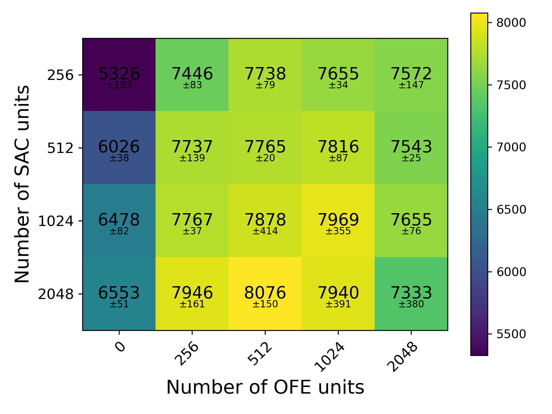
To investigate more in-depth, we also conduct a grid search over different number of units for both SAC and OFENet in Fig. 8. The baseline is SAC agent without OFENet (see leftmost column). The results suggest that the performance does improve when compared against baseline agent (see horizontally), however, it saturates around the average return of . In the following experiments, we employ distributed replay and expect we can attain higher performance.

| SAC | TD3 | ||||||
|---|---|---|---|---|---|---|---|
| Environment | Ours | OFENet | Original | Ours | OFENet | Original | |
| Hopper-v2 | 3467.3 | 3511.6 | 3316.6 | 3206.7 | 3488.3 | 3613.0 | |
| Walker2d-v2 | 8802.4 | 5237.0 | 3401.5 | 7645.8 | 4915.1 | 4515.6 | |
| HalfCheetah-v2 | 19209.9 | 16964.1 | 14116.1 | 18147.5 | 16259.5 | 13319.9 | |
| Ant-v2 | 14021.0 | 8086.2 | 5953.1 | 12811.3 | 8472.4 | 6148.6 | |
| Humanoid-v2 | 14858.2 | 9560.5 | 6092.6 | 13282.0 | 120.6 | 340.5 | |
Distributed RL
Finally, we add distributed replay (Horgan et al., 2018) to further improve performance while using larger networks. We use an implementation similar to (Stooke & Abbeel, 2018), which collects experiences using cores on which each core contains environments, specifically we used and .
Similar to the previous experiments, we conduct a grid search over different number of units for SAC and OFENet with the distributed replay in Fig. 8, and also compare the training curves of three different network size S, M, and L in Appendix B. Comparing Fig. 8 and Fig. 8, we can clearly see the distributed training enables further performance gain on all network size. Furthermore, we can observe monotonic improvement when we increase the number of units for both SAC and OFENet. Thus, we verified combining distributed replay contributes further performance gain while training larger networks.
How about generalization to different RL algorithms and environments?
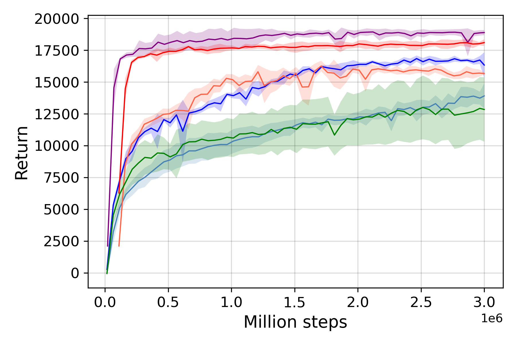
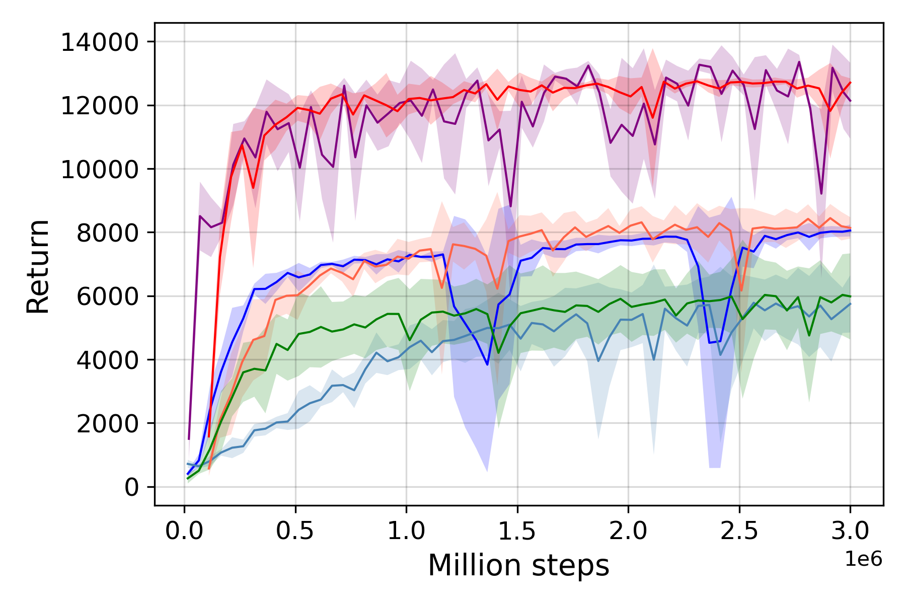
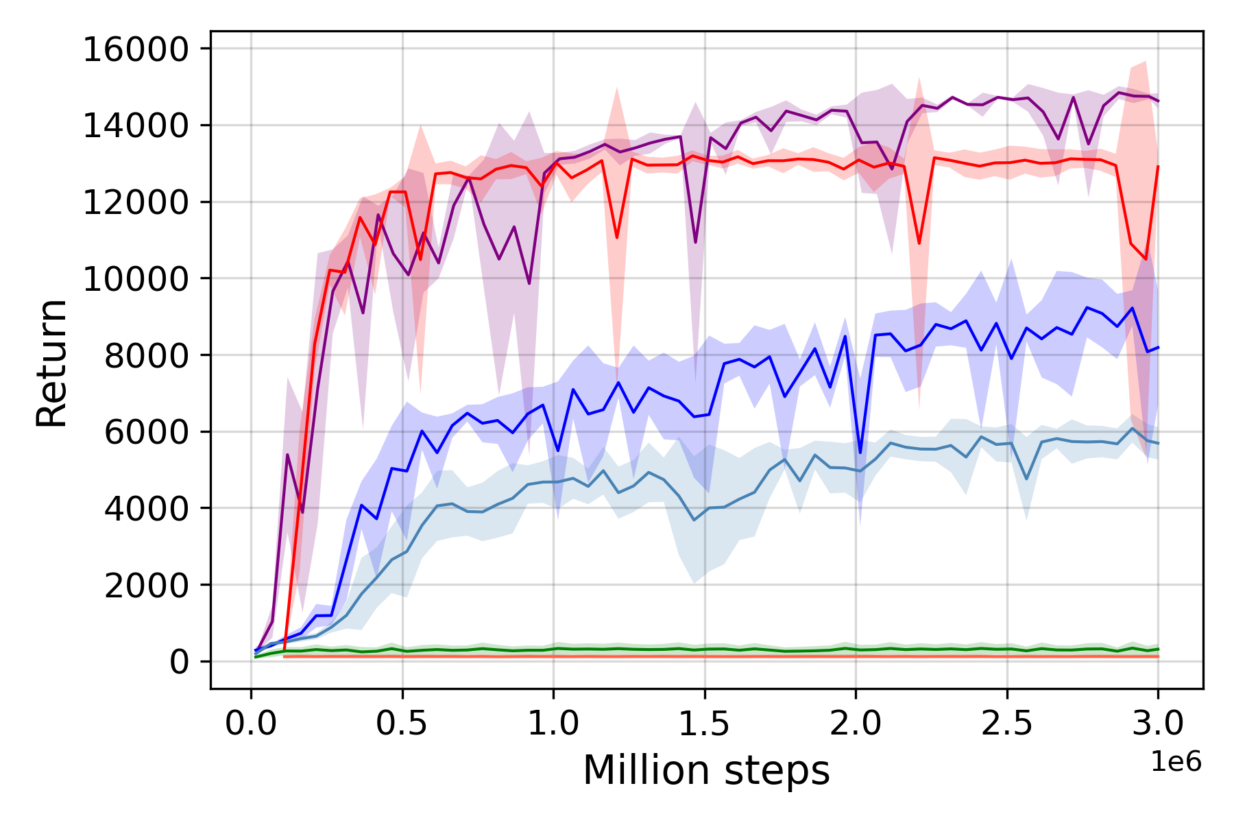
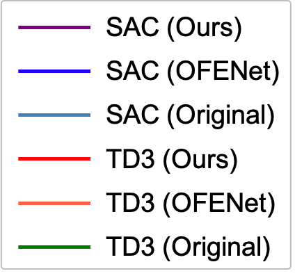
To quantitatively measure the effectiveness of our method across different RL algorithms and tasks, we evaluate two popular optimization algorithms, namely SAC and TD3 (Fujimoto et al., 2018), on five different locomotion tasks in MuJoCo (Todorov et al., 2012). We denote our method as Ours, which uses the largest network of among the previous experiments for both the OFENet and the RL algorithms. We compare the proposed method against two baselines: the original RL algorithm denoted by Original. Furthermore, we also compare OFENet, which can achieve the current state-of-the-art performance on these tasks to the best of our knowledge.
We plot the training curves in Fig. 9 and list the highest average return in Table 1. In the figure and the table, our method, SAC (Ours) and TD3 (Ours) achieves the best performance on almost all environments. Furthermore, we can see that our proposed method can work with both RL algorithms, and thus is agnostic to the choice of the trainign algorithm. In particular, our method notably achieves much higher episode return in Ant-v2 and Humanoid-v2, which are harder environments with larger state/action space and more training examples. Interestingly, the proposed method does not achieve reasonable solutions in Hopper-v2, which has the smallest dimensionality among five environments. We consider that the performance in smaller dimension problem saturates early and even additional methods are unable to provide any significant performance gain.
4.3 Ablation study
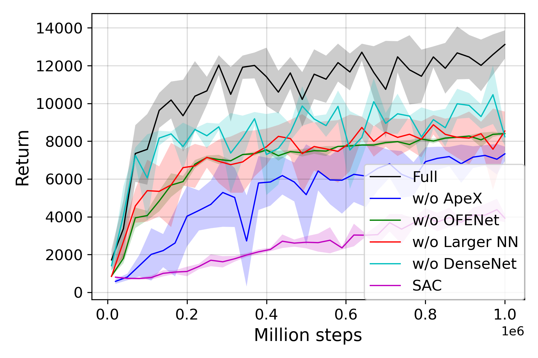
Since our method integrates several different ideas into a single agent, we conduct additional experiments to understand what components contribute to the performance gain. We highlight that our method consists of three elements: feature representation learning using OFENet, DenseNet architecture, and distributed training. In addition to this, we compare the results without increasing the network size to reinforce that larger network does improve performance. Figure 10 shows the ablation study over SAC with Ant-v2 environment. Full is our method which combines all three elements we proposed, and uses large networks () for the SAC agent. sac is the original SAC implementation.
w/o Ape-X removes Ape-X-like distributed training setting. As distributed RL enables collection of more experiences close to the current policy, we consider that the significant performance gain can be explained by learning from more on-policy data, which was also empirically shown by (Fedus et al., 2020). Also, we believe that receiving more novel experiences helps the agent generalize to state-action space. In other words, more novel experience reduces overfitting to limited trajectories, which becomes more important in harder environments which has larger state/action space, and larger neural networks.
w/o OFENet removes OFENet and trains the whole architecture by using only a scalar reward signal. The much lower return shows that learning the large networks from just the scalar reinforcement signal is difficult, and training the bottom networks (close to the input layer), i.e., obtaining informative features by using an auxiliary task enables better learning of control policy.
w/o Larger NN reduces the number of units from to for both OFENet and SAC. This also significantly drops the performance, and thus we can conclude that using larger networks is essential to achieve high performance.
Finally, w/o DenseNet replaces MLP-DenseNet defined in Sec. 3.3 with standard MLP architecture. The result shows that strengthening feature propagation does contribute to improve performance.
5 Conclusion
Deep Learning has catalyzed huge breakthroughs in the fields of computer vision and natural language processing making use of massive neural networks that can be trained with huge amounts of data. While these domains have hugely benefitted from the use of larger networks, the RL community has not witnessed similar trend in use of larger networks for training high performance agents. This is mostly due to instability that occurs when using larger networks for training RL agents. In this paper, we studied the problem of using larger network for training RL agents. To achieve this, we proposed a novel method for training larger networks for deep RL agents while reflecting on some of the important design choices one has to make when using such networks. In particular, the proposed method consists of three elements. First, we decouple representation learning from RL using an auxiliary loss of predicting the next state. This allows to obtain more informative features to be used to learn control policies with richer information compared to learning entire networks from a scalar reward signal. The learned representation is then propagated to the DenseNet architecture that consists of very wide networks. Finally, a distributed training framework provides huge amounts of on-policy data whose distribution is much closer to the current policy, and thus enables to mitigate overfitting problem and enhance generalization to novel scenarios. Our experiments demonstrate that this novel combination achieves significantly higher performance compared against the current state-of-the-art algorithms across different off-policy RL algorithms and different continuous control tasks.
In the future, we would like to study the application to high-dimensional inputs (e.g., images). We also would like to investigate how we can make use of the proposed method for other off-policy methods to make our method agnostic to the choice of underlying algorithm.
References
- Achiam et al. (2019) Achiam, J., Knight, E., and Abbeel, P. Towards characterizing divergence in deep q-learning. 2019.
- Andrychowicz et al. (2021) Andrychowicz, M., Raichuk, A., Stańczyk, P., Orsini, M., Girgin, S., Marinier, R., Hussenot, L., Geist, M., Pietquin, O., Michalski, M., Gelly, S., and Bachem, O. What matters in on-policy reinforcement learning? a large-scale empirical study. In Proceedings of International Conference on Learning Representations (ICLR), 2021.
- Aviral Kumar & Levine (2021) Aviral Kumar, Rishabh Agarwal, D. G. and Levine, S. Implicit under-parameterization inhibits data-efficient deep reinforcement learning. In Proceedings of International Conference on Learning Representations (ICLR), 2021.
- Bengio et al. (1994) Bengio, Y., Simard, P., and Frasconi, P. Learning long-term dependencies with gradient descent is difficult. IEEE Transactions on Neural Networks, 1994.
- Bengio et al. (2007) Bengio, Y., Lamblin, P., Popovici, D., Larochelle, H., et al. Greedy layer-wise training of deep networks. Proceedings of Advances in Neural Information Processing Systems (NIPS), 19:153, 2007.
- Bishop (2006) Bishop, C. M. Pattern Recognition and Machine Learning (Information Science and Statistics). Springer-Verlag, Berlin, Heidelberg, 2006. ISBN 0387310738.
- Brown et al. (2020) Brown, T. B., Mann, B., Ryder, N., Subbiah, M., Kaplan, J., Dhariwal, P., Neelakantan, A., Shyam, P., Sastry, G., Askell, A., Agarwal, S., Herbert-Voss, A., Krueger, G., Henighan, T., Child, R., Ramesh, A., Ziegler, D. M., Wu, J., Winter, C., Hesse, C., Chen, M., Sigler, E., Litwin, M., Gray, S., Chess, B., Clark, J., Berner, C., McCandlish, S., Radford, A., Sutskever, I., and Amodei, D. Language models are few-shot learners. In Larochelle, H., Ranzato, M., Hadsell, R., Balcan, M., and Lin, H. (eds.), Proceedings of Advances in Neural Information Processing Systems (NIPS), 2020.
- Chen et al. (2020) Chen, T., Kornblith, S., Norouzi, M., and Hinton, G. A simple framework for contrastive learning of visual representations. In Proceedings of International Conference on Machine Learning (ICML), pp. 1597–1607, 2020.
- Deng et al. (2009) Deng, J., Dong, W., Socher, R., Li, L., Kai Li, and Li Fei-Fei. Imagenet: A large-scale hierarchical image database. In 2009 IEEE Conference on Computer Vision and Pattern Recognition, 2009.
- Devlin et al. (2019) Devlin, J., Chang, M.-W., Lee, K., and Toutanova, K. BERT: Pre-training of deep bidirectional transformers for language understanding. In Proceedings of the 2019 Conference of the North American Chapter of the Association for Computational Linguistics: Human Language Technologies, Volume 1 (Long and Short Papers), 2019.
- Fedus et al. (2020) Fedus, W., Ramachandran, P., Agarwal, R., Bengio, Y., Larochelle, H., Rowland, M., and Dabney, W. Revisiting fundamentals of experience replay. In Proceedings of the 37th International Conference on Machine Learning, pp. 3061–3071, 2020.
- Fu et al. (2019) Fu, J., Kumar, A., Soh, M., and Levine, S. Diagnosing bottlenecks in deep q-learning algorithms. In Proceedings of International Conference on Machine Learning (ICML), 2019.
- Fujimoto et al. (2018) Fujimoto, S., van Hoof, H., and Meger, D. Addressing function approximation error in actor-critic methods. In Proceedings of International Conference on Machine Learning (ICML), 2018.
- Ha & Schmidhuber (2018) Ha, D. and Schmidhuber, J. Recurrent world models facilitate policy evolution. In Proceedings of Advances in Neural Information Processing Systems (NIPS). 2018.
- Haarnoja et al. (2018) Haarnoja, T., Zhou, A., Abbeel, P., and Levine, S. Soft Actor-Critic: Off-Policy Maximum Entropy Deep Reinforcement Learning with a Stochastic Actor. CoRR, 2018.
- He et al. (2016) He, K., Zhang, X., Ren, S., and Sun, J. Deep residual learning for image recognition. In Proceedings of IEEE Conference on Computer Vision and Pattern Recognition (CVPR), pp. 770–778, 2016. doi: 10.1109/CVPR.2016.90.
- He et al. (2016) He, K., Zhang, X., Ren, S., and Sun, J. Identity mappings in deep residual networks. In Proceedings of European Conference on Computer Vision (ECCV), 2016.
- He et al. (2020) He, K., Fan, H., Wu, Y., Xie, S., and Girshick, R. Momentum contrast for unsupervised visual representation learning. In Proceedings of IEEE Conference on Computer Vision and Pattern Recognition (CVPR), June 2020.
- Henaff (2020) Henaff, O. Data-efficient image recognition with contrastive predictive coding. In Proceedings of International Conference on Machine Learning (ICML), pp. 4182–4192, 2020.
- Henderson et al. (2018) Henderson, P., Islam, R., Bachman, P., Pineau, J., Precup, D., and Meger, D. Deep reinforcement learning that matters. In AAAI, 2018.
- Hernandez et al. (2021) Hernandez, D., Kaplan, J., Henighan, T., and McCandlish, S. Scaling laws for transfer. 2021.
- Hessel et al. (2018) Hessel, M., Modayil, J., van Hasselt, H., Schaul, T., Ostrovski, G., Dabney, W., Horgan, D., Piot, B., Azar, M. G., and Silver, D. Rainbow: Combining improvements in deep reinforcement learning. In AAAI, 2018.
- Horgan et al. (2018) Horgan, D., Quan, J., Budden, D., Barth-Maron, G., Hessel, M., Van Hasselt, H., and Silver, D. Distributed prioritized experience replay. arXiv preprint arXiv:1803.00933, 2018.
- Huang et al. (2017) Huang, G., Liu, Z., Van Der Maaten, L., and Weinberger, K. Q. Densely connected convolutional networks. In 2017 IEEE Conference on Computer Vision and Pattern Recognition (CVPR), pp. 2261–2269, 2017. doi: 10.1109/CVPR.2017.243.
- Ioffe & Szegedy (2015) Ioffe, S. and Szegedy, C. Batch normalization: Accelerating deep network training by reducing internal covariate shift. In Proceedings of International Conference on Machine Learning (ICML), 2015.
- Jaderberg et al. (2017) Jaderberg, M., Mnih, V., Czarnecki, W. M., Schaul, T., Leibo, J. Z., Silver, D., and Kavukcuoglu, K. Reinforcement learning with unsupervised auxiliary tasks. In Proceedings of International Conference on Learning Representations (ICLR), 2017.
- Kapturowski et al. (2019) Kapturowski, S., Ostrovski, G., Dabney, W., Quan, J., and Munos, R. Recurrent experience replay in distributed reinforcement learning. In Proceedings of International Conference on Learning Representations (ICLR), 2019.
- Krizhevsky et al. (2012) Krizhevsky, A., Sutskever, I., and Hinton, G. E. Imagenet classification with deep convolutional neural networks. In Pereira, F., Burges, C. J. C., Bottou, L., and Weinberger, K. Q. (eds.), Proceedings of Advances in Neural Information Processing Systems (NIPS), volume 25, pp. 1097–1105. Curran Associates, Inc., 2012.
- Lesort et al. (2018) Lesort, T., Díaz-Rodríguez, N., Goudou, J.-F., and Filliat, D. State Representation Learning for Control: An Overview. CoRR, 2018.
- Li et al. (2018) Li, H., Xu, Z., Taylor, G., Studer, C., and Goldstein, T. Visualizing the loss landscape of neural nets. In Proceedings of Advances in Neural Information Processing Systems (NIPS), pp. 6391–6401, 2018.
- Liu et al. (2021) Liu, Z., Li, X., Kang, B., and Darrell, T. Regularization matters in policy optimization. In Proceedings of International Conference on Learning Representations (ICLR), 2021.
- Lu et al. (2017) Lu, Z., Pu, H., Wang, F., Hu, Z., and Wang, L. The expressive power of neural networks: a view from the width. In Proceedings of Advances in Neural Information Processing Systems (NIPS), pp. 6232–6240, 2017.
- Mnih et al. (2015) Mnih, V., Kavukcuoglu, K., Silver, D., Rusu, A. A., Veness, J., Bellemare, M. G., Graves, A., Riedmiller, M., Fidjeland, A. K., Ostrovski, G., et al. Human-level control through deep reinforcement learning. Nature, 518(7540):529–533, 2015.
- Munk et al. (2016) Munk, J., Kober, J., and Babuška, R. Learning state representation for deep actor-critic control. In IEEE Conference on Decision and Control (CDC), pp. 4667–4673, 2016.
- Nguyen & Hein (2017) Nguyen, Q. and Hein, M. The loss surface of deep and wide neural networks. In Proceedings of International Conference on Machine Learning (ICML), pp. 2603–2612, 2017.
- Ota et al. (2020) Ota, K., Oiki, T., Jha, D., Mariyama, T., and Nikovski, D. Can increasing input dimensionality improve deep reinforcement learning? In Proceedings of International Conference on Machine Learning (ICML), pp. 7424–7433, 2020.
- Radford et al. (2019) Radford, A., Wu, J., Child, R., Luan, D., Amodei, D., and Sutskever, I. Language models are unsupervised multitask learners. 2019.
- Ramachandran et al. (2017) Ramachandran, P., Zoph, B., and Le, Q. V. Searching for Activation Functions. CoRR, 2017. URL http://arxiv.org/abs/1710.05941.
- Ramchoun et al. (2017) Ramchoun, H., Idrissi, M. A. J., Ghanou, Y., and Ettaouil, M. New modeling of multilayer perceptron architecture optimization with regularization: an application to pattern classification. IAENG International Journal of Computer Science, 44(3):261–269, 2017.
- Schaul et al. (2016) Schaul, T., Quan, J., Antonoglou, I., and Silver, D. Prioritized experience replay. In Proceedings of International Conference on Learning Representations (ICLR), 2016.
- Shelhamer et al. (2017) Shelhamer, E., Mahmoudieh, P., Argus, M., and Darrell, T. Loss is its own reward: Self-supervision for reinforcement learning. In Proceedings of International Conference on Learning Representations (ICLR), 2017.
- Sinha et al. (2020) Sinha, S., Bharadhwaj, H., Srinivas, A., and Garg, A. D2rl: Deep dense architectures in reinforcement learning, 2020.
- Stooke & Abbeel (2018) Stooke, A. and Abbeel, P. Accelerated methods for deep reinforcement learning. arXiv preprint arXiv:1803.02811, 2018.
- Stooke et al. (2020) Stooke, A., Lee, K., Abbeel, P., and Laskin, M. Decoupling representation learning from reinforcement learning, 2020.
- Sutton & Barto (2018) Sutton, R. S. and Barto, A. G. Reinforcement Learning: An Introduction. A Bradford Book, Cambridge, MA, USA, 2018.
- Tan & Le (2019) Tan, M. and Le, Q. Efficientnet: Rethinking model scaling for convolutional neural networks. In Proceedings of International Conference on Machine Learning (ICML), pp. 6105–6114. PMLR, 2019.
- Todorov et al. (2012) Todorov, E., Erez, T., and Tassa, Y. Mujoco: A physics engine for model-based control. In Proceedings of IEEE/RSJ International Conference on Intelligent Robots and Systems (IROS), 2012.
- Van Hasselt et al. (2016) Van Hasselt, H., Guez, A., and Silver, D. Deep reinforcement learning with double q-learning. In Thirtieth AAAI conference on artificial intelligence, 2016.
- van Hasselt et al. (2018) van Hasselt, H., Doron, Y., Strub, F., Hessel, M., Sonnerat, N., and Modayil, J. Deep reinforcement learning and the deadly triad. CoRR, 2018.
- Wu et al. (2019) Wu, Z., Shen, C., and Van Den Hengel, A. Wider or deeper: Revisiting the resnet model for visual recognition. Pattern Recognition, 90:119–133, 2019.
- Zhang et al. (2017) Zhang, C., Bengio, S., Hardt, M., Recht, B., and Vinyals, O. Understanding deep learning requires rethinking generalization. In Proceedings of International Conference on Learning Representations (ICLR), 2017.
Appendix A Experimenal Details
This section describes more details of our experiments.
A.1 Implementation
OFENet
To implement OFENet, we referred the official codebase provided by Ota et al. (2020), which is available at their website111Codes used for implementing MLP-ResNet and MLP-DenseNet can be found at https://www.merl.com/research/license/OFENet. We also employed target networks (Mnih et al., 2015) to stabilize the training of OFENet, since the distribution of experiences stored in the shared replay buffer can change more dynamically by utilizing the Ape-X-like distributed training setting as described in Sec. 3.2. The target networks are updated on each training step by having them slowly track the learned networks: , where we assume to be the network parameters of the current OFENet, and is the parameters of the target network. We use the target smoothing coefficient , which is the same with the one used to update target value networks in SAC (Haarnoja et al., 2018), in other words, we do not tune this parameter.
RL agents
Our implementation of the RL agents are also based on the public codebase used in (Ota et al., 2020). As for Batch Normalization (Ioffe & Szegedy, 2015), which we use for OFENet and TD3 (Ours) in Fig. 9, we use its training mode in updating the network, and test mode in collecting experiences as done in (Liu et al., 2021). We also used Huber loss to stabilize the training of RL agents for the same reason that we employ the target network for training OFENet described in the previous paragraph.
Distributed training
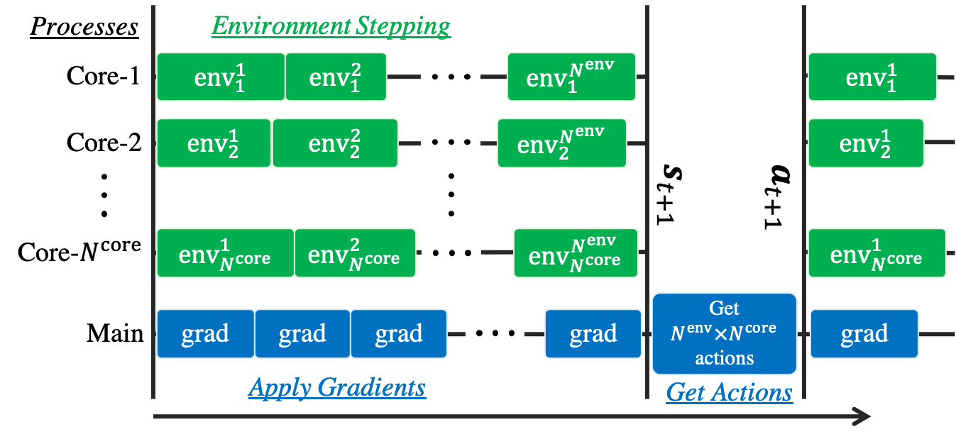
The distributed training setting we used is similar to (Stooke & Abbeel, 2018), which collects experiences using cores on which each core contains environments. Specifically, we used and . Figure 11 shows the schematic of the distributed training. Since the actions are computed by the latest parameters, the collected experiences result in more on-policy data.
A.2 Network Architectures
We highlight that our proposed architecture consists of three elements: 1) Decoupling representation learning from RL using OFENet, 2) DenseNet architecture with large NNs to effectively propagate the features obtained using OFENet, and 3) distributed training to obtain more on-policy experiences that can mitigate overfitting problems and improve performance (see Fig. 2 as well).
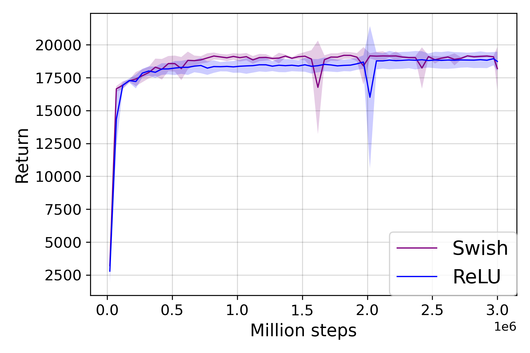
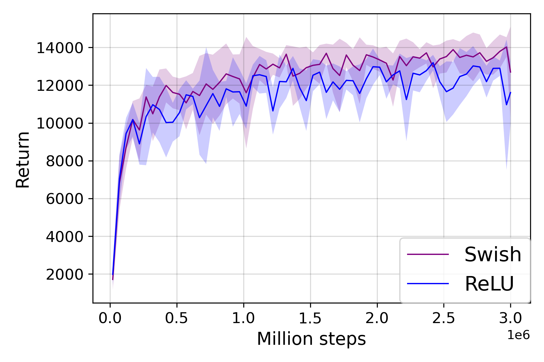
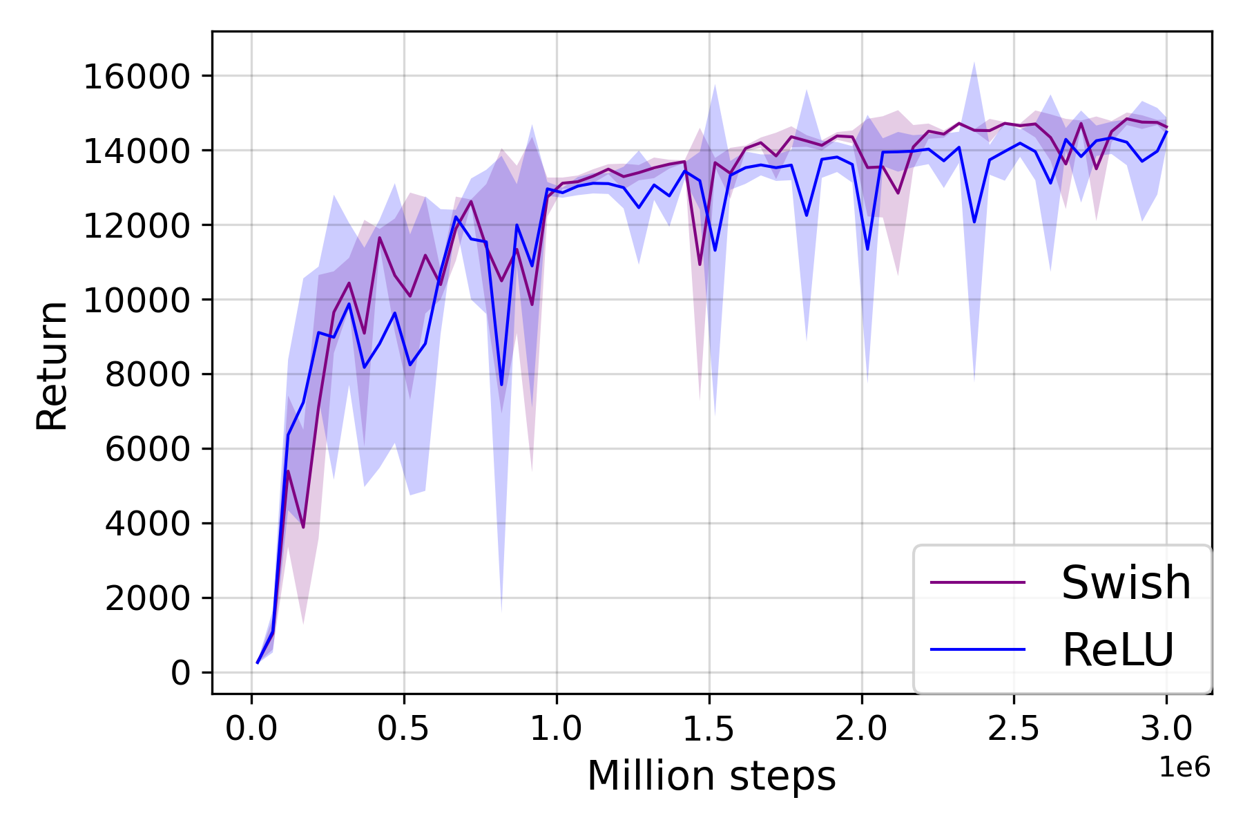
As described in Sec. 3.3, the DenseNet architecture consists of a composite function of fully-connected layer, Batch Normalization, and an activation function. We choose the activation function to be Swish (Ramachandran et al., 2017) for MLP-ResNet and MLP-DenseNet, because it showed the smallest value of the auxiliary loss, i.e. attains the best accuracy of function approximation for predicting the next state on all environments as shown in (Ota et al., 2020). (We compared the performance of RL with different activation functions in Fig. 13)
For OFENet, we designed the architecture to increase the feature dimensionality to from original inputs by using 8-layers DenseNet architecture as proposed in (Ota et al., 2020). For SAC agent, we designed the architecture to concatenate features at each layer. Table 2 shows the number of parameters for SAC (Ours) and SAC (Original) as reference on Ant-v2 environment as an example, which has 111 and 8 dimensionality for state and action space. As you can see from the table, we increase the parameters of the network to be 100 times more than the original SAC implementation.
| SAC (Ours) | SAC (Original) | |||||||
|---|---|---|---|---|---|---|---|---|
| Input | Output | Parameters | Input | Output | Parameters | |||
| units | units | units | units | |||||
| OFENet: | st layer | 29,696 | ||||||
| nd layer | 367 | 95,232 | ||||||
| rd layer | 623 | 160,768 | ||||||
| th layer | 879 | 226,304 | ||||||
| th layer | 1,135 | 291,840 | ||||||
| th layer | 1,391 | 357,376 | ||||||
| th layer | 1,647 | 422,912 | ||||||
| th layer | 1,903 | 488,448 | ||||||
| Total | ||||||||
| SAC | st layer | 2,159 | 2,048 | 4,423,680 | 111 | 256 | 28,672 | |
| nd layer | 4,207 | 2,048 | 8,617,984 | 256 | 256 | 65,792 | ||
| Output layer | 6,255 | 8 | 50,048 | 256 | 8 | 2,056 | ||
| Total | ||||||||
| Total | ||||||||
A.3 Visualizing loss surface of Q-function networks
Li et al. (2018) proposed a method to visualize the loss function curvature by introducing filter normalization method. The authors empirically demonstrated the non-convexity of the loss functions can be problematic, and the sharpness of the loss surface correlates well with test error and generalization error. In light of this, we also visualize the loss surface of the networks to figure out why the deeper network could not lead to better performance while the wider networks result in high performance policies (Fig. 4).
To visualize the loss surface of our Q-networks, we use the authors’ implementation222Code used for these plots can be found at: https://github.com/tomgoldstein/loss-landscape with the loss of:
| (2) |
with
| (3) |
in which we exactly follow the notations used by SAC paper (Haarnoja et al., 2018). To compute this objective , we collect all transitions used in the training of the deeper and wider networks, and compute the target values of after finishing training and stored the tuples of for all transitions in the training. Then, we use the authors’ implementation to visualize the loss with the stored transitions and trained weights of the Q-network. Please refer to (Li et al., 2018) for more details.
A.4 Hyperparameters
OFENet
All OFENet networks we used for our experiments consist of 8-layers DenseNet architectures with Swish activation (Ramachandran et al., 2017) as used in (Ota et al., 2020). The output dimensionality of OFENet is defined in each experiment. Table 2 in the previous section shows the detailed output units in each layer as an example.
RL algorithms
The hyperparameters of the RL algorithms are also the same with their original papers, except that the TD3 uses the batch size instead of as done in (Ota et al., 2020). Also for fair comparison to (Ota et al., 2020), we used a random policy to store transitions to replay buffer before training RL agents for 10K time steps for SAC, and for 100K steps for TD3.
Effective rank
We employ the effective rank, which is recently proposed in (Aviral Kumar & Levine, 2021), as a metric to evaluate the effectiveness of our architecture as described in Sec. 3. Following the notations given by Aviral Kumar & Levine (2021), the effective rank can be computed as , where are the singular values of feature matrix , which is the features of the penultimate layer of the Q-networks. We used to calculate the number of effective ranks in the experiments, as in (Aviral Kumar & Levine, 2021).
Appendix B Additional Results
B.1 Training Curves
Distributed RL
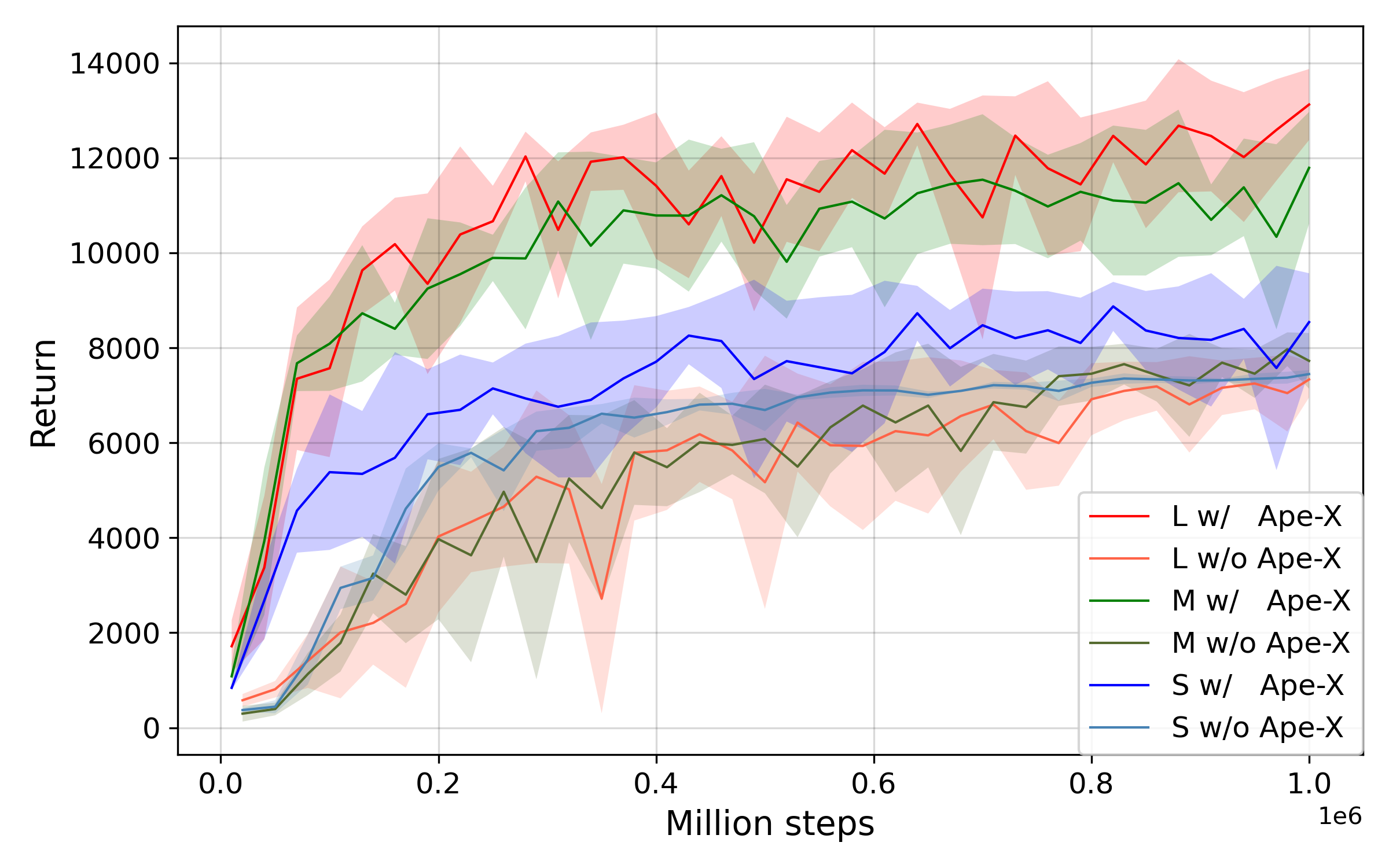
In order to evaluate the performance of distributed RL, we compare the performance of our method w/ and w/o Ape-X-like distributed training over different three network size: , which we respectively denote S, M, and L. We denote the baseline by w/o Ape-X, which are the same with w/ OFENet in Fig. 8. It is noted again that the horizontal axis indicates the number of steps we applied gradients, not environmental steps as we use distributed actors that interact with environments in parallel (see Fig. 2).
Figure 12 shows that using Ape-X enables to improve performance on all network size, and the larger networks tend to further improve the performance.
Activation
As described in Appendix A.2, we used Swish activation for RL agents (policy and value function networks) as it is shown to improve accuracy of function approximation in (Ota et al., 2020). To evaluate the effect of different activation functions, we plot the results of SAC (Ours) with different activation functions (ReLU and Swish) for policy and value function networks used in SAC in Fig. 13. The results show we have slight performance gain by replacing ReLU with Swish. More comprehensive empirical studies can be found in (Andrychowicz et al., 2021; Henderson et al., 2018).
B.2 Loss surface
In addition to showing the loss surface of the deeper and wider networks that are trained on Ant-v2 environment in Fig. 1 and Fig. 4, we also visualize the loss landscapes of Q-networks trained on HalfCheeta-v2 environment in Fig. 14. Together with the results shown in Fig. 1 and Fig. 4, we can see the wider networks tend to converge to a flatter minimum while the deeper networks have sharper minimums.
