Fully general-relativistic simulations of isolated and binary strange quark stars

Abstract

The hypothesis that strange quark matter is the true ground state of matter has been investigated for almost four decades, but only a few works have explored the dynamics of binary systems of quark stars. This is partly due to the numerical challenges that need to be faced when modelling the large discontinuities at the surface of these stars. After adopting a suitable definition of the baryonic mass of strange quark matter (SQM) we introduce a novel technique in which a very thin crust is added to the equation of state of SQM to produce a smooth and gradual change of the specific enthalpy across the star and up to its surface. The introduction of the crust has been carefully tested by considering the oscillation properties of isolated quark stars, showing that the response of the simulated quark stars matches accurately the perturbative predictions. Using this technique, we have carried out the first fully general-relativistic simulations of the merger of quark-star binaries finding several important differences between quark-star binaries and hadronic-star binaries with the same mass and comparable tidal deformability. In particular, we find that the dynamical mass loss is $\sim 20\%$ smaller than that coming from a corresponding hadronic binary. In addition, quark-star binaries have merger and post-merger frequencies that obey the same quasi-universal relations derived from hadron stars if expressed in terms of the tidal deformability, but not when expressed in terms of the average stellar compactness. Hence, it may be difficult to distinguish the two classes of stars if no information on the stellar radius is available. Finally, differences are found in the distributions in velocity and entropy of the ejected matter, for which quark-stars have much smaller tails. Whether these differences in the ejected matter will leave an imprint in the electromagnetic counterpart and nucleosynthetic yields remains unclear, calling for the construction of an accurate model for the evaporation of the ejected quarks into nucleons.

I Introduction

The detection of gravitational waves (GWs) from the coalescence of two compact objects with masses that can be associated to compact stellar objects has been reported recently by the LIGO-Virgo Scientific Collaboration [1, 2, 3]. One of these GW detections, GW170817, was accompanied by an electromagnetic counterpart [4, 5] and has therefore been associated with the merger of a binary system of neutron stars which have long been proposed to be behind the production of short gamma-ray bursts [6, 7, 8, 9]. Furthermore, the detection of a kilonova emission through the ejected material and the subsequent r-process nucleosynthesis [10, 11, 12, 13, 14, 15, 16, 17, 18] has provided further evidence that the GW signal in GW170817 must have been produced by the merger of two compact matter objects.

Combining the knowledge of nuclear physics, general relativity, and numerical relativity simulations, this detection has certainly helped to deepen our understanding of cold dense matter equation of state (EOS) through a tight constraints on maximum mass, radii and tidal deformability of the neutron stars [19, 20, 21, 22, 23, 24, 25, 26, 27, 28, 29, 30, 31]. Besides the more conventional scenario of the merger of purely hadronic compact stars leading to a purely hadronic merged object, other possibilities have been explored in great detail. One of them is the possibility that the merging objects were hybrid (or twin) stars [32, 33, 34, 35, 36, 37, 38], that a phase transition to quark matter could have taken place after the merger [39, 40, 41], or that the merger involved strange-quark stars [42, 43]. All of these different scenarios are in principle compatible with the GW signal of GW170817, which was necessarily limited to the inspiral only.

The solution of the equations of general-relativistic hydrodynamic (GRHD) or general-relativistic magnetohydrodynamic (GRMHD) are indispensable tools for the accurate modelling of these scenarios and the quantitative prediction of the signals produced by the inspiral and merger, be it through the gravitational radiation, the emission of neutrinos, or the ejection of matter.

Over the years, the scenario of the merger of fully hadronic compact stars has been studied by GRHD and GRMHD simulations in great detail [44, 45, 46, 47, 8, 48, 49, 50, 51, 15, 52, 53, 13, 54, 55, 18]. Among the numerous results that have been obtained with these simulations (see [56, 57] for some reviews), two are particularly relevant for the results presented in this work. The first one is about the spectral properties of the GW signal – both during the inspiral and after the merger – have been analysed in great detail and shown to follow quasi-universal relations in terms of the stellar tidal deformability or compactness [58, 59, 60, 61, 62, 63, 64, 65]. The second one is instead related to the matter ejected at merger and after the merger [66, 67, 13, 68, 69, 70, 54, 15, 51, 55, 71], and the impact that it has on r-process nucleosynthesis, on the lifetime of the merged object [72], and on the maximum mass of compact stars [19, 21, 31].

While the fully hadronic scenario has been covered in great detail, the alternative scenarios involving matter in different states – either before or after the merger – has so far been considered less extensively. The few investigations performed so far have in fact been limited to the analysis of the post-merger GW signal when a phase transition sets in after the merger and leads to clear signatures in the GW signal [39, 40, 41]. In particular, these studies have highlighted that differences, sometimes significant, can be found in the post-merge GW spectrum and that the universal relations found in the case of hadronic stars are obviously broken if a considerable quark core is produced.

The literature is even scarcer when it comes to simulations exploring the inspiral and merger of quark-star binaries that composed of pure strange quark matter (SQM). Indeed, the first and only works so far are more than a decade old and have been obtained using smooth particle hydrodynamics and a conformally flat approximation to general relativity [73, 74]. This is in great part due to the considerable additional difficulties that the numerical simulation of these objects implies and that originates from the very sharp decrease in density and enthalpy at the surface of the quark star.

We recall that the SQM hypothesis was firstly proposed by Witten and suggesting that SQM, rather than nuclear matter, is the absolute ground state of matter [75]. In this hypothesis, SQM is mainly composed by up, down, and strange quarks, with a small fraction of electrons also present. Because of the self-bound properties of SQM, objects composed of this matter can exist in any size, from scales as small as those of nuclei, to scales as large as that of a compact star. Indeed, in this hypothesis, a quark star composed of SQM has been proposed as a possible candidate of compact stars. The properties of single quark stars have been studied by numerous works [76, 77, 78, 79, 80, 81, 82, 83, 84, 85, 86, 87, 88], while the study of the binary quark-star mergers have been explored far less [73, 74, 89, 43, 90, 91].

The detection of the kilonova signal AT2017gfo associated with the GW170817 event has been considered by some as a strong evidence against the existence of SQM. This is because the ejected material of a binary quark-star merger would be composed by SQM that – when assumed to be the most stable form of matter – cannot be an efficient source of $r$-process nucleosynthesis. At the same time, recent studies have highlighted that the SQM scenario can be still conciliated with the signal from AT2017gfo if the SQM can evaporate into nucleons as a result of the high temperatures reached after the merger. In this case, most of ejected SQM from the quark-star binary would have evaporated into nucleons and could have therefore contributed to the kilonova signal in AT2017gfo  [90, 92, 93].

With the goal of studying the scenario of the merger of quark stars – and thus explore the possibility of SQM evaporation in far greater detail – we have carried out the first fully general-relativistic simulations of the inspiral and merger of quark stars. Contrasting their evolution with a system of compact stars that have very similar properties in mass and compactness but are fully hadronic, we have been able to isolate three important features of the merger of quarks stars. First, their GW spectral properties are in agreement with the quasi-universal behaviour found for hadronic stars during the inspiral, but differs in the post-merger phase. Second, because of the intrinsic self-boundness of these objects, the amount of ejected mass is smaller, with binary quark stars ejecting $\sim 20\%$ less mass than a corresponding hadronic binary. Finally, as natural to be expected for matter that is colder and more self-bound, the ejected matter contains considerably smaller tails in the corresponding distributions of velocity and entropy.

The structure of the paper is as follows. In Sec. II we discuss in detail the mathematical and physical setup that was necessary to develop in order to carry out the numerical simulations. Section Sec. III is instead dedicated to a careful test of the validity of our approach when considering the oscillation properties of isolated quark and hadronic stars, and their match with perturbative studies. Section  IV is used to present in detail the results of our simulations, including both the overall dynamics of the merger and the outcomes in terms of GW signal and ejected matter. Finally, our conclusions and prospects for future work are presented in Sec. V, while Appendix A provides details on the technique that can be used when considering different values of the baryon mass.

II Mathematical and Numerical Setup

II.1 Equations of state

The EOS of the SQM employed in our simulations was chosen to be the MIT2cfl EOS [42, 94]. This EOS makes use of the MIT bag model with additional perturbative QCD corrections [95, 96, 97, 42], and satisfies the constraints of having a maximum mass above two solar masses as required by the observations [98, 99], and a tidal deformability compatible with the constraints from GW170817. In this EOS a colour-flavor-locked (CFL) phase is assumed to be present and consequently the number densities of all the flavor of quarks [up (u), down (d), and strange (s) quarks] are the same, i.e.,

$$n_{u}=n_{d}=n_{s}\,.$$ (1)

As a result, the baryon number density defined as

$$n_{{}_{\rm B}}\mathrel{\mathop{\mathchar 58\relax}}=\frac{1}{3}(n_{u}+n_{d}+n_{s})\,,$$ (2)

can be directly converted to the rest-mass density $\rho$ that enters in the hydrodynamic equations and is evolved numerically, as $\rho\mathrel{\mathop{\mathchar 58\relax}}=m_{{}_{\rm B}}n_{{}_{\rm B}}$, where $m_{{}_{\rm B}}$ is the average baryonic mass. We note that while the value of $m_{{}_{\rm B}}$ is well defined for a baryon, this is not the case when considering SQM. In particular, we recall that the definition of the baryonic mass for hadronic matter is given by the value of total energy density per baryon at vanishing pressure, i.e.,

$$m_{{}_{\rm B}}\mathrel{\mathop{\mathchar 58\relax}}=\frac{e(p=0)}{n_{{}_{\rm B}}(p=0)}\,.$$ (3)

As a result, when considering the MIT2cfl EOS employed here, we obtain that the baryon mass is $m_{{}_{\rm B}}\simeq 850\,{\rm MeV}$. We note that this value is smaller than the one assumed for hadronic matter, i.e., $940\,{\rm MeV}$ (see, e.g., [92]), but has been employed also by other groups (see, e.g., [73, 100, 101]). Two comments should be made at this point. First, the definition Eq. (3) naturally implies that at zero pressure the specific internal energy is also zero, i.e., $\epsilon(p=0)=0$, so that the specific enthalpy at the stellar surface is $h(p=0)=1+\epsilon+p/\rho=1$, as one would expect. Second, as we will comment in more detail in Appendix A, a different value of the baryon mass inevitably introduces a discontinuity at the stellar surface, thus calling for a suitable rescaling in order to carry out the numerical simulations.

Possibly the most serious challenge in modelling compact stars made of SQM is that – because of their self-bound property – the surface of such objects is characterized by a sharp transition at the stellar surface, where the pressure goes to zero at a nonzero rest-mass density. As a result, a large, intrinsic density jump is present at the stellar surface; by contrast, hadronic stars have surfaces near which the density rapidly decreases, but that goes to zero when the pressure is zero. When considering static solutions, as for example when constructing stellar models of isolated quark stars, such a density jump can be handled analytically by matching the stellar interior with the exterior vacuum  [102, 103, 42, 94]. However, in the context of a hydrodynamic simulation, such a discontinuity represents the exemplary condition for the development of a strong shock that would lead to an artificial oscillation in the best-case scenario or to a numerical failure in the most realistic case. Clearly, a treatment aimed at smoothing this strong discontinuity into a region with small but finite size is necessary for a numerical evolution.

A simple solution at the level of the EOS may consist in the introduction of a polytropic piece in the pressure dependence from the rest-mass density, i.e., $p=k\rho^{\Gamma}$ with $k=8.12$ and $\Gamma=1.90$, thus effectively introducing a thin but nonzero “crust” in the quark star. The presence of a thin crust in a quark star and its implications have been studied in detail in a number of works [104, 105, 106]. The introduction of a crust changes, at least in principle, the tidal deformability. In practice, however, the change is extremely small and of $1.3\%$ only. More precisely, the tidal deformabilities for a quark star with and without crust are 789.3 and 778.9, respectively.

A few important aspects of our novel approach need to be remarked at this point. First, although artificial, the introduction of the thin crust does not provide a perceptible variation to the global properties. While we will demonstrate this in Sec. III, where we will compare the oscillation properties of an isolated star with the perturbative expectations, it suffices to say here that the variation on the gravitational mass after the introduction of thin crust is minute, i.e., $\sim 5\times 10^{-3}\,M_{\odot}$, as is its spatial extension, which is restricted to two grid cells and therefore has a width of $\simeq 240\,{\rm m}$.

Second, since we have introduced a thin crust, our compact star could be assimilated to a “hybrid star” as it is effectively composed of two regions: a quark-matter and a nuclear-matter region, although the latter is extremely thin. Indeed, simulations of this type of compact stars were performed and investigated in great detail in Refs. [107, 108]. However, this similarity is potentially misleading because a strange quark star is actually composed of SQM that represents the ground state at any density. On the contrary, the quark matter in a hybrid star could exist as the ground state only if the density is sufficiently high, namely, at least larger than the saturation density. Hence, we prefer to regard ours as a strange star with a thin crust rather than a hybrid star.

Finally, the handling of the MIT2cfl EOS for the actual merger requires the addition of a thermal part to the EOS. We do this in close analogy with what done routinely for simulations of hadronic stars described by cold EOSs. In essence, we account for the additional shock heating during the merger and post-merger phases by including thermal effects via a “hybrid EOS”, that is, by adding an ideal-fluid thermal component to the cold (subscript “c” below) EOS [109]

$$p = p_{\rm c}+p_{\rm th}\,,$$ (4)

$$p_{\rm th} = \rho\epsilon_{\rm th}(\Gamma_{\rm th}-1)\,,$$ (5)

$$\epsilon_{\rm th} = \epsilon-\epsilon_{\rm c}(\rho)\,,$$ (6)

where $\Gamma_{\rm th}=1.75$ is the thermal adiabatic index.

Since we find it important to contrast the dynamical behaviour of merging quark stars with the corresponding one of hadronic stars with the same total mass, we have also considered the merger of a binary system subject to a hadronic EOS for comparison. Our choice has fallen on the DD2 EOS [110], which is compatible with the present observational constraints, and whose tidal deformability for a $M=1.35\,M_{\odot}$ star is close to that of a quark star of the same mass. At the same time, the radius of the quark star is significantly smaller: $R=11.81\,\rm{km}$ for the MIT2cfl quark star versus $R=13.21\,\rm{km}$ for DD2 hadronic star.

In the framework of a comparative assessment of the dynamics of SQM and hadronic-matter binaries, and despite the fact that the hadronic DD2 EOS is a finite-temperature EOS employed in many GRHD or GRMHD simulations [111, 13, 15, 112, 113], we have adopted a hybrid-EOS approach [cf. Eqs. (4)–(6)] also for the DD2 EOS, of which we have retained only the zero-temperature slice. An immediate disadvantage of this approach is that the consistent knowledge of some thermodynamical quantities, such the temperature or the entropy, are missing and need to be estimated in alternative manners. In this case, additional assumptions – some of which are not necessarily realistic – are required to extract these quantities, at least to some degree. However, since the same approximations are made for both EOSs, the expectation is that the systematic differences we can find in this way will persist also when considering more advanced and temperature-dependent EOSs for SQM.

More specifically, in the case of ideal-fluid EOS, the temperature $T$ is proportional to the average kinetic energy per particle and we can therefore express the specific internal energy $\epsilon$ as

$$\epsilon=\frac{k_{t}T}{m_{{}_{\rm B}}}\,,$$ (7)

where $k_{t}$ is a constant and $m_{{}_{\rm B}}$ is mass per baryon. We extend this expression to our EOSs by rewriting it as

$$\epsilon=k_{t}\frac{(T-T_{\rm c})}{m_{{}_{\rm B}}}+\epsilon_{\rm c}(\rho)\,,$$ (8)

where $T_{\rm c}$ is the temperature of the cold part of the EOS and which we take to be to $T_{\rm c}=0.01\,{\rm MeV}$. Using now Eq. (8) and recalling that for transformations at constant density $d\epsilon=Tds$, we can compute the specific entropy as

$$s=\frac{k_{t}}{m_{{}_{\rm B}}}\log\left(\frac{\epsilon-\epsilon_{\rm c}}{k_{t}T_{\rm c}/m_{{}_{\rm B}}}+1\right)\,.$$ (9)

Finally, specifying $k_{t}=20$ for both EOSs, we can compute the entropy per baryon $s_{{}_{\rm B}}=m_{{}_{\rm B}}s$ once $\epsilon$ and $\epsilon_{\rm c}$ are known.

II.2 Numerical setup: Initial data

The initial data for binary stars was generated making use of the publicly available Lorene code [114], which is a multi-domain spectral-method code computing quasi-equilibrium irrotational binary configurations of compact stars. Using this code, and as discussed above, we have computed initial binary configurations of both quark stars and of hadronic stars. Independently of whether we have considered the $\rm{MIT2cfl}$ or the $\rm{DD2}$ EOS, the properties of the binary have been set to be the same: the initial separation in the binary was set to be $45\,{\rm km}$ and the two stars have the same mass of $M=1.35\,M_{\odot}$.

It is useful to remark that the introduction of a thin crust for the quark star was important also for the calculation of the initial data. Furthermore, the computation of the solution of binary quark stars with Lorene required extra care. In particular, because of the steep drop in rest-mass density across the crust of the quark star and of the presence of discontinuities in higher-order derivatives at the crust-core interface (we recall that the EOS is continuous but with discontinuous derivatives at crust-core interface), a single interior coordinate domain employed to cover the quark star turned out to be insufficient and prevented the convergence to an accurate solution. Fortunately, however, the addition of a second domain at higher resolution to cover the crust was sufficient to yield the convergence to an accurate solution.

Table 1: Properties of the quark and hadron stars considered here, and distinguished in whether they refer to the isolated configurations or to binaries. Reported are the mass $M$, the baryon mass $M_{b}$, the radii $R$, and the tidal deformability $\Lambda$. In addition, in the case of the binaries, we also report the relevant frequencies of the gravitational-wave signal ($f_{\rm max},f_{1}$, and $f_{2}$), the ejected matter $M_{\rm ej}$ and the ejected baryon number $N_{\rm B}^{\rm ej}$.

		Quark star	Hadronic star
${\rm EOS}$	${\rm type}$	${\rm MIT2cfl}$	${\rm DD2}$
$M\ [M_{\odot}]$	$({\rm isolated})$	$1.40$	$1.40$
$M_{b}\ [M_{\odot}]$	$({\rm isolated})$	$1.57$	$1.53$
$R\ [{\rm km}]$	$({\rm isolated})$	$11.90$	$13.22$
$\Lambda$	$({\rm isolated})$	$657.78$	$698.72$
$M\ [M_{\odot}]$	$({\rm binary})$	$1.35$	$1.35$
$M_{b}\ [M_{\odot}]$	$({\rm binary})$	$1.50$	$1.47$
$R\ [{\rm km}]$	$({\rm binary})$	$11.81$	$13.21$
$\Lambda$	$({\rm binary})$	$789.32$	$857.69$
$f_{\rm max}\ [{\rm kHz}]$	$({\rm binary})$	$1.684$	$1.644$
$f_{1}\ [{\rm kHz}]$	$({\rm binary})$	$1.919$	$1.845$
$f_{2}\ [{\rm kHz}]$	$({\rm binary})$	$2.399$	$2.436$
$M_{\rm ej}\ [10^{-3}\,M_{\odot}]$	$({\rm binary})$	$2.68$	$2.94$
$N_{\rm B}^{\rm ej}\ [10^{54}]$	$({\rm binary})$	$3.520$	$3.533$

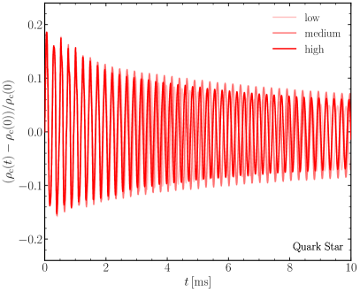
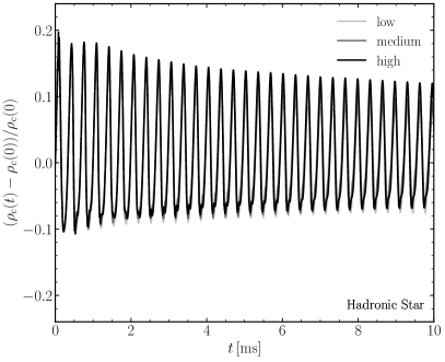
Figure 1: Evolutions of the normalised variations in the stellar central rest-mass density $\rho_{c}(t)$ for either an oscillating quark star (left panel) or for a hadronic star (right panel). Curves of different shading refer to different resolutions, with the high-resolution data being shown with the darkest shade.

II.3 Numerical setup: evolution equations

The simulations presented here have been performed with the publicly available GRHD code WhiskyTHC [115, 116, 117], which is a high-order, fully general-relativistic code for the solution of the equations of relativistic hydrodynamics and compatible with the Einstein Toolkit [118]. The hydrodynamic equations were solved by using a high-resolution shock-capture (HRSC) [109] approach having with Local Lax-Friedrichs (LLF) flux-split and Monotonicity Preserving 5th-order (MP5) reconstruction method [119, 120] under the finite-difference scheme. The spacetime was instead evolved by implementing the CCZ4 formulation [121, 122] through the finite-differencing code McLachlan [123].

In order to cover a large enough spatial domain and hence compute accurately the information on the ejected matter while keeping a high resolution on the compact stars, an adaptive-mesh refinement (AMR) approach was employed and handled by the CARPET driver [124]. The number of refinement levels depends on the problem considered and was of $3$ levels in the case of isolated stars and of $6$ levels in the case of merging binaries. In this way, the corresponding total extents of the computational domain were set to $24\,M_{\odot}\ (36\,{\rm km})$ and $2048\,M_{\odot}\ (3051\,{\rm km})$, respectively. Furthermore, each of the scenario considered – isolated stars or binary mergers – has been evolved with simulations at different resolutions. More specifically, for the finest grid we have used three resolutions in the case of isolated stars, i.e., $dx=0.16\,M_{\odot}\ (236\,{\rm m})$, $dx=0.12\,M_{\odot}\,(177\,{\rm m})$, and $dx=0.08\,M_{\odot}\ (118\,{\rm m})$, which we will indicate as “low”, “medium”, and “high” resolution in following. Similarly, for both quark and hadronic stars, we have employed two resolutions in the case of merging binaries, i.e., $dx=0.25\,M_{\odot}\ (369\,{\rm m})$ and $dx=0.16\,M_{\odot}\ (236\,{\rm m})$, which we will indicate as “low” and “high”, respectively. Note that a resolution of $dx=0.16\,M_{\odot}\ (236\,{\rm m})$, and even lower ones, (see e.g., [125, 126]) have been used routinely in simulations of binary neutron stars and has been shown to be sufficient to capture accurately the dynamics of the system.

III Results: isolated quark stars

As a first but very important test of the correct implementation of the rescaling procedure presented in the previous Section, we next discuss the results from the evolution of isolated and oscillating quark stars, comparing with the corresponding evolutions obtained with fully hadronic stars. The analytical formulation and the numerical computation of the spectral properties of oscillating compact stars is a very old one and has been studied in detail in the literature [127, 128, 129, 130], also in the case of quark stars [86, 88]. Similarly, the investigation of the dynamical response of a relativistic star to a perturbation has been studied extensively in the literature (see, e.g., [131, 132, 133] for some of the initial works).

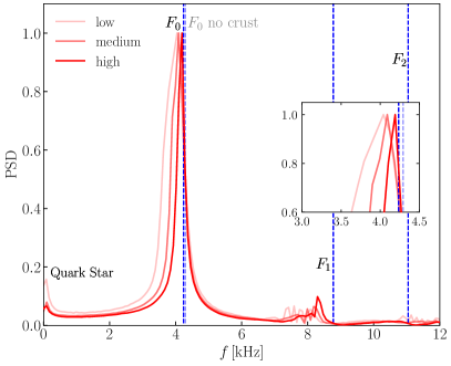
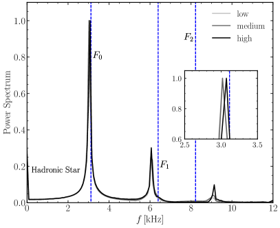
Figure 2: Power spectral densities of the timeseries in Fig. (1) when compared with the perturbative predictions for the eigenfrequencies, reported as vertical blue dashed lines. The left panel refers to a quark star, while the right one to a hadronic star; the same convention is followed for the different types of lines. In both cases, the insets show a magnification near the frequency of the $F_{0}$ mode. Note that the accuracy of the match increases as the resolution is increased.

Because this serves only as a test and not to study the spectral properties of such stars, the oscillations we have considered are simple quasi-radial oscillations of initially static stars, whose perturbative eigenfrequencies of can be obtained easily by solving two ordinary differential equations [see Eqs. (11)–(12) in Ref. [88]] that are coupled with the equations of stellar equilibrium, i.e., the Tolmann-Oppenheimer-Volkoff (TOV) equations (see, e.g., [109]). To make the comparison meaningful, both the isolated MIT2cfl quark stars and the hadronic DD2 stars have the same mass of $M=1.4\,M_{\odot}$. Solving the perturbation equations together with the TOV equations, we obtain the eigenfrequencies $F_{i}$, for different mode numbers $i$. In practice, we limit ourselves to the fundamental model $F_{0}$ and the first overtone $F_{1}$. Note that both the static models and the eigenfrequencies are computed after introducing the crustal prescription in the EOS, as described in the previous Section. For the dynamical evolutions, on the other hand, we introduce an initial purely radial perturbation in the radial velocity with an eigenfunction corresponding to an $n=1$, $\ell=0$ oscillation mode under the Cowling approximation (i.e., with a spacetime being held fixed) [134], and an amplitude of $3\%$.

As customary, we report in Fig. 1 the normalised variation in the stellar central density $\rho_{c}(t)$ for either the quark star as discussed above (i.e., with a thin crust, left panel) or for the hadronic star (right panel). Curves of different shading refer to different resolutions, with the high-resolution data being shown with the darkest shade. Note that, especially for the quark star, the behaviour of the oscillations shows aspects of strong nonlinearity, i.e., deviation from a simple harmonic oscillation, during the first few millisecond, but these then disappear rather soon and the oscillation becomes rather regular. As to be expected, these nonlinear features becomes more marked as the resolution is increased and the deviations from a perfect conservation of rest-mass are $\lesssim 10^{-5}\%$.

Note also the imprint of different resolutions is more evident in the quark star than in the hadronic one. A phase difference can in fact be measured in the low- and medium-resolution evolutions for the quark star, which is instead absent for the hadronic star. This is again easy to interpret as due to the much sharper density jump at the stellar surface in the case of a quark star, which requires therefore a higher resolution to produce a consistent behaviour. However, for both stars, the low resolution is sufficient to capture a convergent behaviour and the accuracy simply increases as the resolution is increased. Finally, it should be noted that while the quark star exhibits oscillations that are almost symmetric with respect to the unperturbed value, the hadronic one does not. This is due to the fact that for the latter, the oscillations are accompanied by a significant contribution from higher-order modes (see discussion below).

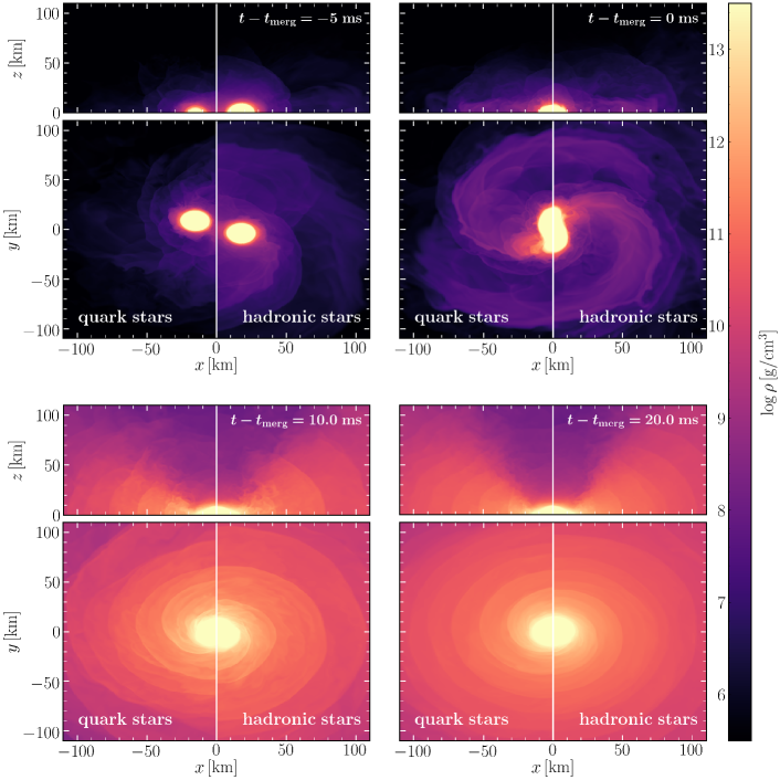
Figure 3: Small-scale (i.e., $110\,{\rm km}$) views of the rest-mass density at different but characteristic times during the merger of the two classes of binaries [i.e., $5\,{\rm ms}$ before merger (upper-left), the merger time (upper-right), $10\,{\rm ms}$ (lower left), and $20\,{\rm ms}$ (lower right) after merger]. Each panel offers views of the $(x,y)$ plane (bottom parts) and of the $(x,z)$ plane (top parts), respectively. Note that, for each panel, the left part refers to quark stars, while the right one to the hadronic stars.

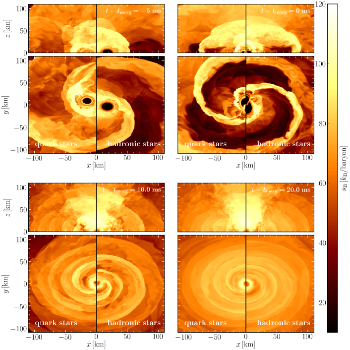
Figure 4: Same as in Fig. 3, but for the entropy per baryon.

Figure 2 helps to compare and contrast the evolutions of quark and hadron stars by taking the Fourier transforms of the timeseries in Fig. (1) and comparing the resulting power spectral densities (PSDs) with the perturbative prediction for the eigenfrequencies, reported as vertical blue dashed lines. In this way, it is apparent that the match between the dynamical and the perturbative results is worse for the quark star, especially at low resolutions (see the insets). However, as the resolution is increased, both evolutions nicely converge to the perturbative values and differ from them with comparable errors, namely, $1.1\%$ ($3.1\%$) and $1.3\%$ ($3.5\%$) for the quark and hadron stars at high (medium) resolution, respectively. Note also that the low-resolution of the quark star has a considerable amount of noise near the position of the $F_{1}$ frequency, but that this noise decreases with increasing resolution, leading to the clear appearance of an overtone in the high-resolution run. Finally, note that the amount of power in the two overtones is much larger in the case of the hadronic star, which exhibits a clear second overtone. This behaviour in indeed visible already in the timeseries reported in Fig. 1 (right panel), which exhibits rapid variations near the maxima and minima of the oscillations. Also reported for a comparison and marked with a transparent blue dashed line is the $F_{0}$ eigenfrequency of a strange star without a crust; note that this is larger and that the simulation do not converge to this value.

In summary, the results presented here on the dynamics of isolated quark stars show that the approach presented in Sec. II.1 to handle the stellar surface is not only properly implemented, but that it also leads to evolutions that are able to reproduce the spectral properties of quark stars and yield numerically consistent evolutions. At the same time, they show that, in general, quark stars require higher resolutions than the ones that would be needed for a hadronic star with comparable properties in terms of mass and tidal deformability. Once again, this is the inevitable drawback of having to model stars with a strong self-confinement and sharper density profiles at the surface.

IV Results: binary quark stars

In this section we discuss the dynamics of a binary quark-star merger and contrast it with the corresponding merger obtained with a hadronic EOS. Before entering in the details, and notwithstanding that these are the first fully general-relativistic simulations of the merger of SQM compact objects, it is useful to stress what are the limitations of our approach. First, the treatment of the thermal part of the EOS is necessarily approximate and modeled with a hybrid EOS approach for both EOSs [cf. Eqs. (4)–(6)]. As a result of this (forced) choice, the modelling of neutrinos, e.g., via a leakage [135], or more advanced approaches [50, 136], is not possible. Second, the modelling of the quark-evaporation processes in the ejected matter, is de-facto ignored. While both processes are expected to have a significant impact on the electromagnetic kilonova signal and on the nucleosynthesis, they are not expected to play an important role in the gravitational-wave signal, which can therefore be considered robust. Third, for obvious computational costs, the two resolutions used here for the binaries are rather low, and the highest one would correspond to the “low” resolution in the case of the isolated stars discussed in the previous Section. However, as demonstrated above, such a resolution is sufficient to provide a sufficiently accurate description of the stellar behaviour given that the relative error in the PSD for the low-resolution quark star is $\lesssim 4.6\%$. More importantly, by comparing and contrasting quark and hadronic stars with similar properties we can easily capture – even at these low resolutions – the systematic differences between the two stellar types, which we believe are therefore robust.

IV.1 Overview of the dynamics

The main features of the dynamics of the binary systems of quark and hadronic stars are rather similar. Before the merger, the stars in the binary systems inspiral towards each other as a result of energy and angular moment loss via gravitational-wave emission. During this stage, the matter effects are dominated by the tidal deformability of the two stars. This stage is shown in the top-left panels of Figs. 3–4, which report the small-scale (i.e., $110\,{\rm km}$) views of the rest-mass density (Fig. 3) or of the entropy per baryon (Fig. 4). Different panels refer to different but characteristic times during the merger [i.e., $5\,{\rm ms}$ before merger (upper-left), the merger time (upper-right), $10\,{\rm ms}$ (lower left), and $20\,{\rm ms}$ (lower right) after merger] and offer views of the $(x,y)$ plane (bottom parts) and of the $(x,z)$ plane (top parts), respectively. More importantly for our comparison, for each panel, the left part refers to quark stars, while the right one to the hadronic stars. While not straightforward to analyse, Figs. 3–4 are rich of information and help obtain a comprehensive overview of the properties of the dynamics of the two binaries.

It should be noted that already in the inspiral phase, the quark-star binary loses a smaller amount of material from the surface. While this matter is not significant both in terms of gravitational-wave emission and nucleosynthesis (the material has very small velocities, is distributed essentially isotropically, and is gravitationally bound in good part), it already shows a feature we will encounter again below.

As the two stars approach each other, the amplitude of the emitted gravitational waves increases, achieving a maximum when the stars merge. At this point in time, intense tidal forces and strong shocks induce a significant and dynamical ejection of matter (see upper-right panels of Fig. 3). After merger, a differentially rotating object is produced whose mass is larger than the maximum mass of rotating configuration and that is normally referred to as hypermassive neutron star (HMNS) in the case of hadronic EOSs, but that should dubbed hypermassive quark star (HMQS) in the case of the MIT2cfl EOS (see lower-left and lower-right panels of Fig. 3).

The dynamics of this post-merger phase is again rather similar between the two EOSs and follows well-known behaviours in terms of dynamical ejecta, tidal forces and shock heating (see, e.g., [13, 15, 137]). In particular, the dynamical ejection of matter takes place mostly at low latitudes (i.e., near the equatorial plane, as it can be seen in the $(x,z)$ sections of Fig. 3). On the other hand, the material at high latitudes (i.e., near the polar directions, as it can be seen in the $(x,z)$ sections of Figs. 4) is considerably hotter and with a higher entropy per baryon. Furthermore, strong shocks taking place in the HMQS and in the HMNS lead to a pulsed dynamical mass ejection, which is apparent in the $(x,y)$ sections of Figs. 3, 4, where it appears in terms of a striped spiral-arm structure. Essentially all of this matter is gravitationally unbound and by being both hot and with high entropy, it will be involved in the subsequent nucleosynthetic processes that cannot be modeled here.

Overall, when inspecting the full set of Figs. 3–4, it is apparent that although no major qualitative difference emerges – as one would have expected given the very similar bulk properties of the components in the two binaries – there are some quantitative differences in the dynamics of quark-star binaries and hadron-star binaries. Postponing a more detailed comparison to Sec. IV.3, we can already appreciate a first important result of our comparative study: mass loss is smaller in SQM binaries than in hadronic binaries. On the other hand, the differences in temperature and entropy are much smaller and of a factor of a few, at most.

IV.2 Gravitational-wave emission

The emission of gravitational waves from merging binaries of compact objects is obviously one of the most interesting outcomes of these processes and can be used to extract important information on the status of matter when these compact objects are stars. It is therefore natural to investigate whether the gravitational-wave signal computed in our simulations can be exploited to distinguish the dynamics of strange quarks stars from that of hadronic stars.

As customary, we can compute the strongest component of the gravitational-wave signal by extracting the $\ell=m=2$ mode of the Weyl-curvature scalar $\psi_{4}$ from our simulations, so that the GW amplitudes in the corresponding mode and in the two polarization $+$ and $\times$ can be obtained by integrating $\psi_{4}$ twice in time

$$h^{22}_{+}-ih^{22}_{\times}=\int^{t}_{-\infty}dt^{\prime}\int_{-\infty}^{t^{\prime}}dt^{\prime\prime}(\psi_{4})_{22}\,.$$ (10)

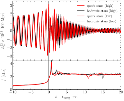
Figure 5: Top panel: gravitational-wave strain in the $\ell=2=m$ mode and in the $+$ polarisation, $h^{22}_{+}$. Curves of different shading refer to different resolutions, with the high-resolution data being shown with the darkest shade. The vertical black line marks the merger time, which corresponds to the time of maximum amplitude, and is used to align the waveforms in phase. Bottom panel: instantaneous gravitational-wave frequencies relative to the strain in the top panel. The same convention is followed for the line types.

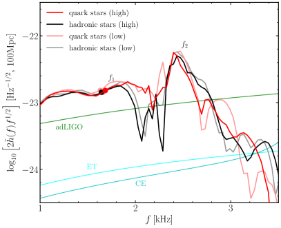
Figure 6: Effective PSDs of the quark-star (red lines) and hadron-star binaries (black lines) at different resolutions. Also reported with filled circles are the frequencies at merger $f_{\rm max}$, as well as the sensitivity curves of advanced and next-generation gravitational-wave detectors such as advanced LIGO (adLIGO), the Einstein Telescope (ET), or Cosmic Explorer (CE). Note the presence of precise spectral features, $f_{1}$ and $f_{2}$, whose frequencies are shown in Table 1.

Figure 5, reports in its top panel the gravitational-wave strains $h^{22}_{+}$ for both the quark-star binary (red lines) and the hadron-star binary (black). As in previous figures, different shades refer to the two resolutions employed, with the high resolutions being indicated with a full shading. The various waveforms are aligned at the time of the merger, that is, the time when the amplitude reaches its first maximum. The bottom part of Fig. 5, on the other hand, reports, the corresponding evolution of the instantaneous gravitational-wave frequencies using the same convention for the line types. Overall, the gravitational-wave information provided in Fig. 5 remarks that the inspiral part of the binary dynamics is very similar between the two types of stars, with the frequency evolutions that are essentially the same in this phase and up to the merger. However, small differences do develop after the merger and, as we will comment below, they can be used to extract important signatures on the occurrence of the merger of a quark-star binary.

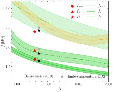
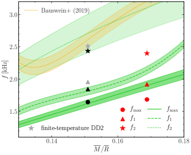
Figure 7: Left panel: Quasi-universal relations for the frequency at merger $f_{\rm max}$ and the two post-merger frequencies $f_{1}$ and $f_{2}$ when shown as a function of the tidal deformability $\Lambda$ ([cf. Eqs. (13), (IV.2), and (17)]). Shown with symbols are the values of the frequencies measured from the high-resolution simulations in the case of quark-star binaries (red symbols) or hadron-star binaries (black symbols). Reported for comparison with gray symbols are the frequencies when considering the temperature-dependent version of the DD2 EOS. Right panel: same as in the left panel but when the quasi-universal relations are expressed in terms of the average stellar compactness $\mathcal{C}$ ([cf. Eqs. (LABEL:eq:f1_2) and (18)]). In both panels the shading refers to the uncertainties in the relations and the orange lines report the functional fitting in Ref. [40].

In order to highlight the differences that emerge after the merger we follow the methodology presented in Ref. [63] to process the post-merger GW signal and perform a spectral analysis whose results are shown in Fig. 6. First of all, we collect the GW signal in the time interval $t\in[-1500,4000]\,M_{\odot}\sim[-7.39,19.70]\,{\rm ms}$, and perform a Fourier transformation with a symmetric time-domain Tukey window function, with parameter $\alpha=0.25$. This window function helps eliminating spurious oscillations of the computed PSD. Furthermore, since we are interested only in the post-merger signal, we employ a fifth-order high-pass Butterworth filter for the low-frequency part of the signal with a cutoff frequency set to be $f_{\rm cut}=f(t-t_{\rm merg}=-7.38\,{\rm ms})+0.5\,{\rm kHz}$. In this way we compute the effective PSD as [63]

$$\tilde{h}(f)\mathrel{\mathop{\mathchar 58\relax}}=\sqrt{\frac{|\tilde{h}_{+}(f)|^{2}+|\tilde{h}_{\times}(f)|^{2}}{2}}\,,$$ (11)

where $\tilde{h}_{+}(f)$ and $\tilde{h}_{\times}(f)$ are the Fourier transforms of the to two gravitational-wave strains. At the same time, it is possible to compute signal-to-noise ratio (SNR) as

$${\rm SNR}\mathrel{\mathop{\mathchar 58\relax}}=\left[\int_{0}^{\infty}\frac{|2\tilde{h}(f)f^{1/2}|^{2}}{S_{h}(f)}\frac{df}{f}\right]^{1/2}\,,$$ (12)

where $S_{h}(f)$ is the noise PSD of a given gravitational-wave detector.

Figure 6 reports the effective PSDs of the two binaries (red and black lines for the quark-star and the hadron-star binaries, respectively) at the two different resolutions (dark and light shading for the high and low resolutions, respectively), and the frequencies at merger $f_{\rm max}$ (filled circles; these frequencies are also used to match the amplitudes of the PSDs obtained at different resolutions). Also reported in Fig. 6 are the sensitivity curves of advanced and next-generation gravitational-wave detectors such as advanced LIGO (adLIGO), the Einstein Telescope (ET) [138, 139], or Cosmic Explorer (CE) [140]. In this way, it is possible to appreciate the presence of precise spectral frequencies, i.e., gravitational-wave spectral lines, which are named as $f_{1}$ and $f_{2}$ after the convention in [141], and whose values are shown in Table 1. Also reported as filled solid circles on top of the various PSDs are the gravitational-wave frequencies at the merger (i.e., at amplitude maximum) $f_{\rm max}$. Note that a third frequency, $f_{3}$ can be obtained from the approximate relation $2f_{2}\approx f_{1}+f_{3}$, which models the dynamics of the two stellar cores in terms and repeated collisions and bounces while the HMNS/HMQS rotates.

As first pointed out in Ref. [59], the values of $f_{\rm max}$ can be used as an important proxy of the EOS. Furthermore, this frequency was shown to follow a quasi-universal behaviour in terms of the tidal deformability. On the other hand, both Fig. 5 and Fig. 6 clearly indicate that the values of $f_{\rm max}$ are rather similar for both quark and hadronic stars. This is because, although the radii of the stars in the two binaries are rather different, i.e., $R_{{}_{\rm QS}}\simeq 11.8\,{\rm km}$ and $R_{{}_{\rm HS}}\simeq 13.2\,{\rm km}$ for the quark (QS) and hadron star (HS), respectively (see Table 1), the corresponding tidal deformabilities are very similar, i.e., $\Lambda_{{}_{\rm QS}}\simeq 790$ and $\Lambda_{{}_{\rm HS}}\simeq 860$. Indeed, in Ref. [64] and using a large set of purely hadronic EOSs, a universal relation was found between the $f_{\rm max}$ and tidal deformability, namely

$$\log_{10}\left(\frac{f_{\rm max}}{{\rm Hz}}\right)\approx a_{0}+a_{1}\Lambda^{1/5}-\log_{10}\left(\frac{2\overline{M}}{M_{\odot}}\right)\,,$$ (13)

where $a_{0}=4.186,a_{1}=-0.140$, and $\overline{M}$ represent the average mass at infinite separation (in our simulations and for both binaries, $\overline{M}=1.35\,M_{\odot}$).

The quasi-universal relation (13) is shown with a green solid line in the left panel of Fig. 7 as a function of the tidal deformability $\Lambda$ and in the right panel as a function of the average stellar compactness $\mathcal{C}\mathrel{\mathop{\mathchar 58\relax}}=\overline{M}/\overline{R}$, where $\overline{R}$ is the average radius. We recall that this is possible because another quasi-universal relation exists relating the tidal deformability $\Lambda$ with the stellar compactness $\mathcal{C}$, namely [142, 143]

$$\mathcal{C}=0.360-0.0355\,\ln\Lambda+0.000705\,(\ln\Lambda)^{2}\,.$$ (14)

Also shown in Fig. 7 with red and black symbols are the values of the measured gravitational-wave frequencies at merger $f_{\rm max}$ for binary quark stars (red filled circles) and binary hadronic stars (black filled circles), respectively. When comparing the numerical results with the expected quasi-universal relation with the tidal deformability (left panel of Fig. 7), it is clear that the match is very good despite the very different nature of the two binaries and, in particular, the large difference in radii. This result may appear bizarre at first as one would expect that the gravitational-wave frequency at merger is directly related to the stellar radius and indeed the “contact” frequency is normally computed as the Keplerian frequency when the two stars have a separation which is twice the stellar radius $f_{\rm cont}\mathrel{\mathop{\mathchar 58\relax}}=\mathcal{C}^{3/2}/(2\pi\overline{M})$ [144, 141]. However, as recently pointed out in Ref. [145], the gravitational-wave frequency at merger $f_{\rm max}$ is closely related to the quadrupolar ($\ell=2$) $F$-mode oscillation ($F_{2F}$) of nonrotating and rotating models; furthermore, $F_{2F}$ is can also be expressed quasi-universally in terms of the tidal deformability, so that the results shown in the left panel of Fig. 7 are essentially stating that quark and hadronic stars with similar tidal deformability – and thus similar properties of their dense cores – have similar quadrupolar $F_{2F}$ oscillation modes and, hence, similar gravitational-wave frequency at merger $f_{\rm max}$. This is another important result of our comparative study: quark-star binaries have merger frequencies similar to those of hadron-star binaries with comparable tidal deformability. In turn, this implies that it may be difficult to distinguish the two classes of stars based only on the gravitational-wave signal during the inspiral.

Note, however, that when expressed in terms of the stellar compactness (see right panel of Fig. 7), the match between the measured merger frequencies and the expectations from the quasi-universal relations is reasonably good in the case of hadronic stars, but it is much worse for quark-star binaries. This hints to the fact that while expression (13) could be used both for hadronic and quark-star binaries, the corresponding expression in terms of the stellar compactness needs to be corrected in the case of quark-star binaries. We will return to this point below.

Figure  7 also shows additional quasi-universal relations for the $f_{1}$ and $f_{2}$ frequencies, both as a function of the tidal deformability (left panel) and of the average stellar compactness (right panel). For the first, low-frequency peak, the universal relations are expressed respectively as [63, 64]

$$f_{1} \approx b_{0}+b_{1}\,\mathcal{C}+b_{2}\,\mathcal{C}^{2}+b_{3}\mathcal{C}^{3}\ {\rm kHz}\,,$$

$$f_{1} \approx c_{0}+c_{1}\,\Lambda^{1/5}+c_{2}\,\Lambda^{2/5}+c_{3}\,\Lambda^{3/5}\ {\rm kHz}\,,$$

where $b_{0}=-35.17,b_{1}=727.99,b_{2}=-4858.54,b_{3}=10989.88,c_{0}=45.19,c_{1}=-31.11,c_{2}=7.50$, and $c_{3}=-0.61$. Similarly, for the second and most powerful feature in the post-merger spectrum, we use [64]

$$f_{2} \approx 5.832-0.800\,\Lambda^{1/5}\ {\rm kHz}\,.$$ (17)

$$f_{2} \approx 5.832-123.016\exp\left({-\sqrt{56.738\,\mathcal{C}+4.930}}\right)\ {\rm kHz}\,,$$ (18)

where for the second relation (18) we have used expression (14). These frequencies are shown in Fig. 7 with green lines and shadings together with their uncertainties are estimated in Ref. [64]; furthermore, they are complemented by the expression for the $f_{2}$ frequency proposed in Eq. (1) of Ref. [40], where it is dubbed $f_{\rm peak}$ (orange line and shading).

A comparison with numerical data clearly shows that the universal relations provide a rather accurate representation in the case of hadronic stars, both when expressed in terms of the tidal deformability (left panel) and of the average stellar compactness (right panel). The match remains very good also in terms of quark stars, but only when the universal relations are given in terms of the tidal deformability (in the case of the $f_{1}$ frequencies, the relative differences are of $2.15\%$ and $0.22\%$ for binary quark stars and binary hadron stars, respectively). Furthermore, the match of the $f_{2}$ frequency of the hadron-star binary (black filled star) with the quasi-universal relation is only marginally acceptable when using expressions (17) and (18), while it is below the value estimated by Ref. [40] (reported for comparison with gray symbols are the frequencies when considering the temperature-dependent version of the DD2 EOS). However, the differences can be quite substantial when the numerical data for binary quark stars is compared with expressions (IV.2), (LABEL:eq:f1_2) for the $f_{1}$ frequency or with expressions (17), (18) for the $f_{2}$ frequency.

We can summarise these findings into another notable result of our comparative investigation: quark-star binaries have post-merger frequencies that obey quasi-universal relations derived from hadron-star binaries in terms of the tidal deformability, but not when expressed in terms of the average stellar compactness. Hence, it may be difficult to distinguish the two classes of stars based only on the post-merger frequencies and if no information on the stellar radius is available. As conjectured above, this behaviour seems to suggest that new universal relations in terms of the stellar compactness need to be derived when consider binaries of SQM. This conjecture can only be verified when simulations with other EOSs for the SQM have been performed.

IV.3 Properties of the ejected material

As mentioned in the Introduction, besides gravitational waves, another important product of the merger of a binary system of compact stars is represented by the ejected matter as this plays an important role in subsequent nucleosynthesis and in the kilonova emission. We have also already remarked that the lack of a consistent treatment of the evaporation process of SQM to nucleons prevents us from establishing what is the actual role played by the ejected matter from the binary quark-star merger. We recall that the study of Ref. [90] has concluded that only a small amount of quark matter can survive evaporation and thus survive to yield a very low density of SQM in the galaxy. At the same time, the use of a hybrid-EOS approach to handle the thermal effects in the hadronic DD2 EOS – and that we have employed to achieve a consistent picture with the MIT2cfl EOS – prevents us from making considerations on the nucleosynthetic yields and kilonova emission also for the binary hadron-star merger.

Notwithstanding these limitations, we can nevertheless obtain interesting comparative measurements of the ejected matter in terms of bulk properties, such as: the total amounts of ejected rest-mass for the two classes of stars and the corresponding distributions in velocity and entropy. To this scope, and as done routinely in this type of simulations, we place a series of detectors in terms of spherical coordinate 2-spheres at different distances from the origin and measure the amount of matter that crosses such detectors. In this way, considering gravitationally unbound the matter satisfying the so-called “geodesic” criterion, namely, matter whose covariant time component of the four-velocity is $u_{t}<-1$ (see [146] for a detailed discussion of various criteria for unbound matter) we can measure the effective mass lost by the binaries. This is shown as a function of time from the merger in Fig. 8 for a detector placed at a radius of $500\,M_{\odot}\simeq 750\,{\rm km}$, where lines of different colours follow the same convention of the previous figures. When comparing the results of the ejected mass from the quark-star binaries and from the hadron-star binaries, the difference is apparent, with the former having $M_{\rm ej}=2.68\times 10^{-3}\,M_{\odot}$ and the latter $M_{\rm ej}=2.94\times 10^{-3}\,M_{\odot}$.

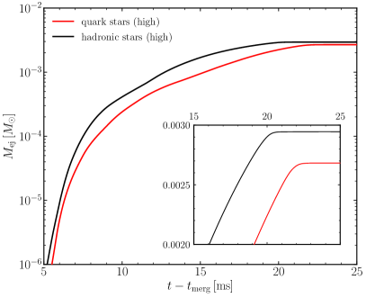
Figure 8: Ejected rest-mass as a function of time as measured by a detector placed at a radius of $500\,M_{\odot}\simeq 750\,{\rm km}$. Lines of different colours follow the same convention of the previous figures: red for quark-star binaries and black for hadron-star binaries. Note that the data refers to the high-resolution simulations and that the ejected mass for the quark-star binaries is smaller.

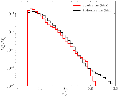
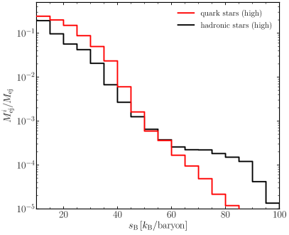
Figure 9: Distributions of the ejected matter in terms of the norm of the three-velocity (left panel) and of the entropy per baryon (right panel). Lines of different colours follow the same convention of the previous figures: red for quark-star binaries and black for hadron-star binaries. Note that the data refers to the high-resolution simulations and that quark-star binaries have much reduced tails in both quantities.

There are at least two explanations behind this difference. The first is that, as mentioned repeatedly, SQM is characterised by self-bound properties and generally harder to eject. Second, quark stars are intrinsically more compact and hence the merged object will be subject both to stronger dynamical shocks but also produce stronger gravitational fields from which it is harder to eject matter. Third, and most importantly, a rest-mass difference is present between SQM and hadronic matter. We recall, in fact, that the average rest-mass per baryon of SQM we adopt here $850\,{\rm MeV}$, which is smaller than the corresponding value for hadronic matter, $940\,{\rm MeV}$.

Proceeding further in our comparison, we report in Fig. 9, two distributions of the ejected matter in terms of the norm of the three-velocity (left panel) and in terms of entropy per baryon (right panel). Note that both distributions are relative to the ejected matter and hence provide a measure of the fraction of the ejecta with given properties. Concentrating first on the left panel, it is clear that the two distributions are very similar and that differences appear only in the high-velocity tails, i.e., $v\gtrsim 0.6$, which are larger by almost one order of magnitude in the case of binary hadron-star mergers. Although the actual amount of matter in these tails is tiny (i.e., $\lesssim 10^{-8}\,M_{\odot}$), they could play a role when interacting with the interstellar medium and produce a re-brightening of the afterglow signal [147] (see [18] for a discussion about the role of fast ejecta).

When considering instead the distribution in entropy (right panel of Fig. 9) – and bearing in mind that the these measurements are the same for the two classes of stars but equally approximate – it is possible to appreciate that quark-star mergers overall produce ejected matter with larger entropy. At the same time, hadron-star mergers are able to eject matter with very high entropy, i.e., $s_{{}_{\rm B}}\gtrsim 60\,k_{{}_{\rm B}}/{\rm baryon}$, and about one order of magnitude more than quark-star mergers. These differences on the entropy distributions may have a potential effects on the subsequent kilonovae observation, but the degree to which this will happen remains unclear until the quark-evaporation mechanism is properly taken into account, more sophisticated EOSs are devised to estimate the impact of SQM in binary mergers, and more systematical investigations are carried out.

V Conclusion

Since the hypothesis that SQM is the ground state of matter has been formulated more than four decades ago, a vast literature has been developed to investigate this scenario and consider its viability against the astronomical observations. In this way, a very large number of works have been presented in which the possibility that SQM could lead to compact stars, i.e., quark stars, has been explored in the greatest detail. Of this vast literature, however, only a very small fraction has been dedicated to the study of the dynamics of binary systems of quark stars. The scarcity of studies of this scenario, which is particularly striking after the detection of gravitational waves and of electromagnetic counterparts from the merger of low-mass compact binaries such as GW170817, probably has a double origin. From an observational side, there is the expectation that a merger of binary quark stars cannot be responsible of the observed kilonova emission in GW170817 and of the subsequent nucleosynthesis. From a theoretical side, on the other hand, the modelling of the inspiral and merger of a binary of quark stars is particularly challenging as it is difficult to properly capture the large discontinuity that appears at the surface of these self-bound stars.

The first of these difficulties has been recently addressed in a number of recent works that have invoked a quark-evaporation process into hadrons that could have taken place as a result of the high temperatures reached after the merger. In this case, therefore, most of ejected SQM from the quark-star binary would have evaporated into nucleons and therefore could have contributed to the kilonova signal in AT2017gfo [90, 92, 93]. Addressing the second difficulty, on the other hand, is the purpose of this work, where we have presented a suitable definition of the baryonic mass of SQM and a novel technique in which a very thin crust has been added to the EOS to produce a smooth and gradual change of the specific enthalpy across the crust. The new approach also allows to use different values for the baryonic mass, which can be introduced via a suitable rescaling of the hydrodynamical variables that are evolved.

The introduction of this crust, whose rest-mass content is minute, i.e., $\sim 5\times 10^{-3}\,M_{\odot}$, and whose spatial extension is restricted to two grid cells only, has been carefully tested by considering the oscillation properties of isolated quark stars. In this way, it was possible to show that the dynamical and simulated response of the quark stars matches accurately the perturbative predictions and that the match becomes increasingly accurate as the numerical resolution is increased. This validation, which has been introduced numerous times in the past when considering neutron stars, has levels of accuracy that are comparable with those obtained with hadronic stars.

Using this novel technique we have been able to carry out the first fully general-relativistic simulations of the merger of binary strange quark stars. In addition, in order to best assess the feature of this merging process that are specific to quark stars, we have carried out a systematic comparison of the dynamics of quark-star binaries with the corresponding behaviour exhibited by a binary of hadron stars having the same mass and very similar tidal deformability, namely, a binary described by the DD2 EOS. In this way, it was possible to highlight several important differences between the SQM and the hadronic stars, which represent the main results of our work. First, the dynamical mass lost is $\sim 20\%$ smaller than that coming from a corresponding hadronic binary. Second, quark-star binaries have merger frequencies similar to those of hadron-star binaries with comparable tidal deformability. Hence, it may be difficult to distinguish the two classes of stars based only on the gravitational-wave signal during the inspiral. Third, quark-star binaries have post-merger frequencies that obey quasi-universal relations derived from hadron-star binaries in terms of the tidal deformability, but not when expressed in terms of the average stellar compactness. Hence, it may be difficult to distinguish the two classes of stars based only on the post-merger frequencies and if no information on the stellar radius is available. Fourth, the matter ejected from quark-star binaries has much smaller tails in the velocity distributions, i.e., for $v\gtrsim 0.6$; this lack of fast ejecta may be revealed by the corresponding lack of a radio re-brightening when the fast ejecta interact with the interstellar medium. Finally, while quark-star binaries eject material that, on average, has larger entropy per baryon, it also lacks the important tail of very high-entropy material. Determining whether these differences in the ejected will able to leave an imprint in the electromagnetic counterpart and nucleosynthetic yields remains unclear.

The results presented here had to rely necessarily on a number of simplifying assumptions and can therefore be improved in a number of ways. First, by adopting EOSs for the SQM that have a proper treatment of the temperature dependence and a nonzero electron fraction. Doing so will allow us not only to accurately and self-consistently describe the thermodynamical evolution after the merger, but also to determine whether the ejected material will lead to the observed chemical abundances. Second, by employing a larger class of EOSs so that it will be possible to establish whether the frequency at merger and the post-merger frequencies obey new universal relations when expressed in terms of the stellar compactness. Finally, and most importantly, by adopting a detailed and quantitative description of the quark-evaporation mechanism, so that a consistent assessment can be made of the viability of binary quark-star mergers as sources to the electromagnetic counterpart in AT2017gfo. All of these improvements will be explored and presented in future works.

x

Appendix A On the value of the baryon mass

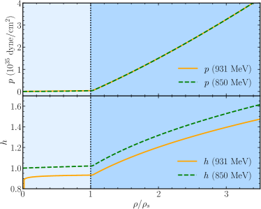
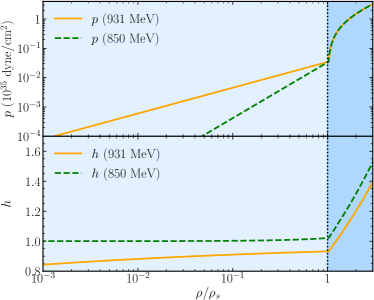
Figure 10: Left panels: behaviour of the pressure $p$ (top part) and of the specific enthalpy $h$ (bottom part) of the MIT2cfl EOS shown as a function of the rest-mass density normalised to the nominal (i.e., without a crust) value at the surface $\rho/\rho_{s}$. The values presented refer to the original pressure (orange solid lines) and to the rescaled one [cf. Eq. (20)] (green dashed lines). Note the appearance of a small jump in $h$ for very small densities. Right panels: same in the right panels, but when the rescaled rest-mass density is shown in a logarithmic scale to highlight the smoother transition.

This appendix is dedicated to some considerations about the value assumed for the baryon mass and what needs to be taken into account if different choices are made. We start this discussion by recalling that the introduction of thin crust modelled with a polytropic EOS requires a certain amount of care as it is necessary to ensure that proper physical conditions are present at the interface between the crust and the SQM. This interface will behave as a contact discontinuity, with jump condition across it given by the continuity of pressure and specific enthalpy, i.e.,  [109]

$$\llbracket p\rrbracket=\llbracket h\rrbracket=0\,,$$ (19)

where $\llbracket\phi\rrbracket$ measures the jump of the scalar function $\phi$ across the contact discontinuity. Clearly, if $\llbracket h\rrbracket\neq 0$, a pressure jump will develop, which will blow away the surface layers of the quark star into the atmosphere.

Clearly, if such a jump in the specific enthalpy is not removed, the quark star will rapidly diffuse away into the atmosphere, thus preventing a numerical evolution. However, since the specific enthalpy $h$ depends on the value of baryonic mass $m_{{}_{\rm B}}$, a potential jump in $h$ at the stellar surface can be removed by a suitable rescaling of the baryon mass. In particular, if we were interested in adopting the value of the baryon mass normally adopted to describe hadronic matter, namely, $m_{{}_{\rm B}}=940\,{\rm MeV}$ – which is also sometimes used to mark the mass of strange quark matter (see, e.g., [92]) – then we would have to face the appearance of a small but nonzero jump in $h$ at the stellar surface.

This is shown in Fig. 10, which reports with a solid orange line the behaviour of the pressure (top panels) and of the specific enthalpy (lower panels) as a function of the rest-mass density normalized to the putative rest-mass density at the surface of the star (i.e., before the addition of a crust), $\rho_{s}$, when assuming a baryon mass $\tilde{m}_{{}_{\rm B}}=940\,{\rm MeV}$. The left panels, in particular, adopt a linear scale in $\rho/\rho_{s}$, while the right panels a logarithmic scale to highlight different properties of the EOS. Note from the bottom-left panel that a jump in $h$ is present near $\rho/\rho_{s}\simeq 0$ and a small part of the star even has a unphysical value of the enthalpy, i.e., $h<1$.

While these results already suggest that such value of the baryon mass should not be considered, a simple rescaling of all of relevant hydrodynamical quantities allows one in principle also to employ $\tilde{m}_{{}_{\rm B}}=940\,{\rm MeV}$. In practice, defining as “core” whatever is the genuine interior of the quark star, it is possible to operate a rescaling within the core of the rest-mass density, of the specific enthalpy, and of the specific internal energy $\epsilon$ of the type

$$\rho\to\rho_{\rm eff}\,, h\to h_{\rm eff}\,, \epsilon\to\epsilon_{\rm eff}\,,$$ (20)

where

$$\rho_{\rm eff} \mathrel{\mathop{\mathchar 58\relax}}=\chi\rho=\chi m_{{}_{\rm B}}n_{{}_{\rm B}}\,,$$ (21)

$$h_{\rm eff} \mathrel{\mathop{\mathchar 58\relax}}=\frac{h}{\chi}\,,$$ (22)

$$\epsilon_{\rm eff} \mathrel{\mathop{\mathchar 58\relax}}=\frac{1+\epsilon}{\chi}-1\,,$$ (23)

while the energy density and pressure are left unchanged, i.e., $e_{\rm eff}=e$, $p_{\rm eff}=p$. In essence, through this rescaling we effectively introduce an effective and larger baryon mass $m_{{}_{\rm B}}^{\rm eff}\mathrel{\mathop{\mathchar 58\relax}}=\chi\tilde{m}_{{}_{\rm B}}=940\,{\rm MeV}$, where $\chi=940/850\simeq 1.11$ such that $h_{\rm eff}=1$ and $\llbracket h_{\rm eff}\rrbracket=0$ at the stellar surface.

The rescaling in Eqs. (21)–(23) described above is done only at the level of the numerical solution of the GRHD equations and to remove the difficulties introduced by the sharp jump at the stellar surface. However, after the completion of each timestep, all the physical quantities entering, for instance, on the right-hand-side of the Einstein equations, are evaluated with the physically correct value of $m_{{}_{\rm B}}$ and hence yield the physically contributions to the energy-momentum tensor.

Combining Eqs. (23) with the thermal part of EOS, one can easily derive the effective quantities of cold part

$$p_{\rm eff,c} =p_{\rm c}\,,$$ (24)

$$h_{\rm eff,c} =\frac{h_{\rm c}}{\chi}\,,$$ (25)

$$\epsilon_{\rm eff,c} =\frac{1+\epsilon_{\rm c}}{\chi}-1\,.$$ (26)

The treatment of the EOS within the crust, on the other hand, remains the same as before, namely, with a single polytrope joining from the stellar surface down to the values of the density associated with the atmosphere (see top-right panel).

The rescaling procedure described above has a simple and direct impact on the equations of relativistic hydrodynamics that we solve numerically. Adopting a flux-conservative formulation of the GRHD equations, the conservation of rest-mass, energy, and momentum can be cast into an “effective” Valencia formulation

$$\partial_{t}(\sqrt{\gamma}\bm{U}_{\rm eff}) = \partial_{i}(\sqrt{\gamma}\bm{F}^{i}_{\rm eff})=\bm{S}_{\rm eff}\,,$$ (27)

where we have employed the rescaling in Eqs. (21)–(23)

$$\bm{U}_{\rm eff} \mathrel{\mathop{\mathchar 58\relax}}= \begin{pmatrix}D\\ S_{j}\\ E\end{pmatrix}=\begin{pmatrix}\rho_{\rm eff}W\\ \rho_{\rm eff}h_{\rm eff}W^{2}v_{j}\\ \rho_{\rm eff}h_{\rm eff}W^{2}-p_{\rm eff}\end{pmatrix}\,,$$ (28)

$$\bm{F^{i}}_{\rm eff} \mathrel{\mathop{\mathchar 58\relax}}= \begin{pmatrix}\alpha v^{i}D-\beta^{i}D\\ \alpha S^{i}_{\ j}-\beta^{i}S_{j}\\ \alpha S^{i}-E\beta^{i}\end{pmatrix}\,,$$ (29)

$$\bm{S}_{\rm eff} \mathrel{\mathop{\mathchar 58\relax}}= \begin{pmatrix}0\\ \alpha S^{ik}\partial_{j}\gamma_{ik}/2+S_{i}\partial_{j}\beta^{i}-E\partial_{j}\alpha\\ \alpha S^{ij}K_{ij}-S^{j}\partial_{j}\alpha\end{pmatrix}\,,$$ (30)

and where $S^{ij}\mathrel{\mathop{\mathchar 58\relax}}=\rho_{\rm eff}h_{\rm eff}W^{2}v^{i}v^{j}+p_{\rm eff}\gamma^{ij}$. Note that the quantities $\gamma_{ij}$, $\gamma$, $\alpha$, $\beta^{i}$, and $K^{ij}$ are, respectively, the spatial three-metric, its determinant, the lapse function, the shift vector, and the extrinsic curvature.

Note that $\gamma_{ij}$, $\alpha$, $\beta^{i}$, and $K^{ij}$ are related to the spacetime metric, which is computed from the Einstein equations via the energy-momentum tensor that is always computed from un-rescaled quantities; hence, these spacetime variables are unaffected by the rescaling operated in the EOS. Similarly, the quantities $S^{i}$, $E$, and $S^{ij}$ all depend on the product $\rho_{\rm eff}h_{\rm eff}$, where the scaling cancels out (i.e., $\rho_{\rm eff}h_{\rm eff}=\rho h$), or on the pressure that is not the rescaled in the core (i.e., $p_{\rm eff}=p$); hence they are not modified by the rescaling. Similarly, the three-velocity $v^{i}$ and the corresponding Lorentz factor $W\mathrel{\mathop{\mathchar 58\relax}}=(1-v^{i}v_{i})^{-1/2}$ are unaffected by the rescaling in the EOS. Consequently, the whole set of GRHD equations (27)–(30) remains unchanged in the core under the rescaling. The only exception is represented by the first equation of the set, i.e., the one involving the conservation of rest-mass. However, since the only change is in the effective baryon mass – which appears in the conservation equation just as a multiplicative constant – the change is practically trivial.

A couple of remarks before concluding this appendix. First, the rescaling in Eqs. (21)–(23) described above is done only at the level of the numerical solution of the GRHD equations and to remove the difficulties introduced by the sharp jump at the stellar surface. However, after the completion of each timestep, all the physical quantities entering, for instance, on the right-hand-side of the Einstein equations, are evaluated with the physically correct value of $m_{{}_{\rm B}}$ and hence yield the physically contributions to the energy-momentum tensor. Second, while $\chi$ is essentially arbitrary and just depends on the value chosen for $\tilde{m}_{{}_{\rm B}}$, it is essential that condition of contact discontinuity Eq. (19) is fulfilled at the stellar surface and that the specific enthalpy at the stellar surface approaches unity.

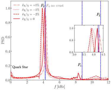
Figure 11: Same as Fig. 2, but when considering values of the scaling parameter $\chi$ differing by a few percent from the reference value.

In order to explore the level of flexibility in varying the value of the scaling constant $\chi$, we have performed simulations of isolated strange stars in which we have varied $\chi$ by a few percent with respect to its reference value. The results of this study are summarised in Fig. 11, which is similar to the left panel of Fig. 2, but reports the PSD when increasing $\chi$ by $1\%$ (i.e., $\delta\chi/\chi=1\%$, red dot-dashed line) or decreasing it by $1\%$ ($\delta\chi/\chi=-1\%$, red dotted line), while performing the simulation at the highest resolution. A rapid inspection of the figure reveals that smaller (larger) value of the scaling constant yield eigenfrequencies that are smaller (larger) than the expected value (red solid line) and that a difference in $\chi$ of only $1\%$ is sufficient to produce differences in the eigenfrequencies of $6\%$. Furthermore, when decreasing $\chi$ further (e.g., $\delta\chi/\chi=-2\%$ as in the red dashed line) the differences with the perturbative results become even more severe and when $\delta\chi/\chi=2\%$ the specific enthalpy is below unity at the surface, preventing a numerical evolution. Finally, we note that because varying the value of $\chi$ effectively changes the slope of the polytropic EOS employed in the crust, and hence its thickness, increasing $\chi$ effectively corresponds to making the crust thinner, thus explaining why the evolution with slightly smaller value of $\chi$ leads to an eigenfrequency that approaches the value of $F_{0}$ for a strange star without crust.