Parallel tempering on optimized paths

Abstract

Parallel tempering (PT) is a class of Markov chain Monte Carlo algorithms that constructs a path of distributions annealing between a tractable reference and an intractable target, and then interchanges states along the path to improve mixing in the target. The performance of PT depends on how quickly a sample from the reference distribution makes its way to the target, which in turn depends on the particular path of annealing distributions. However, past work on PT has used only simple paths constructed from convex combinations of the reference and target log-densities. This paper begins by demonstrating that this path performs poorly in the setting where the reference and target are nearly mutually singular. To address this issue, we expand the framework of PT to general families of paths, formulate the choice of path as an optimization problem that admits tractable gradient estimates, and propose a flexible new family of spline interpolation paths for use in practice. Theoretical and empirical results both demonstrate that our proposed methodology breaks previously-established upper performance limits for traditional paths.

1 Introduction

Markov Chain Monte Carlo (MCMC) methods are widely used to approximate intractable expectations with respect to un-normalized probability distributions over general state spaces. For hard problems, MCMC can suffer from poor mixing. For example, faced with well-separated modes, MCMC methods often get trapped exploring local regions of high probability. Parallel tempering (PT) is a widely applicable methodology (Geyer, 1991) to tackle poor mixing of MCMC algorithms.

Suppose we seek to approximate an expectation with respect to an intractable target density $\pi_{1}$. Denote by $\pi_{0}$ a reference density defined on the same space, which is assumed to be tractable in the sense of the availability of an efficient sampler. This work is motivated by the case where $\pi_{0}$ and $\pi_{1}$ are nearly mutually singular. A typical case is where the target is a Bayesian posterior distribution, the reference is the prior—for which i.i.d. sampling is typically possible—and the prior is misspecified.

PT methods are based on a specific continuum of densities $\pi_{t}\propto\pi_{0}^{1-t}\pi_{1}^{t}$, $t\in[0,1]$, bridging $\pi_{0}$ and $\pi_{1}$. This path of intermediate distributions is known as the power posterior path in the literature, but in our framework it will be more natural to think of these continua as a linear paths, as they linearly interpolate between log-densities. PT algorithms discretize the path at some $0=t_{0}<\dots<t_{N}=1$ to obtain a sequence of densities $\pi_{t_{0}},\pi_{t_{1}},\dots,\pi_{t_{N}}$. See Figure 1 (top) for an example of a linear path for two nearly mutually singular Gaussian distributions.

Given the path discretization, PT involves running $N+1$ MCMC chains that together target the product distribution $\pi_{t_{0}}\pi_{t_{1}}\cdots\pi_{t_{N}}$. Based on the assumption that the chain $\pi_{0}$ can be sampled efficiently, PT uses swap-based interactions between neighbouring chains to propagate the exploration done in $\pi_{0}$ into improved exploration in the chain of interest $\pi_{1}$. By designing these swaps as Metropolis–Hastings moves, PT guarantees that the marginal distribution of the $N^{\text{th}}$ chain converges to $\pi_{1}$; and in practice, the rate of convergence is often much faster compared to running a single chain (Woodard et al., 2009). PT algorithms are extensively used in hard sampling problems arising in statistics, physics, computational chemistry, phylogenetics, and machine learning (Desjardins et al., 2014; Ballnus et al., 2017; Kamberaj, 2020; Müller & Bouckaert, 2020).

Notwithstanding empirical and theoretical successes, existing PT algorithms also have well-understood theoretical limitations. Earlier work focusing on the theoretical analysis of reversible variants of PT has shown that adding too many intermediate chains can actually deteriorate performance (Lingenheil et al., 2009; Atchadé et al., 2011). Recent work (Syed et al., 2019) has shown that a nonreversible variant of PT (Okabe et al., 2001) is guaranteed to dominate its classical reversible counterpart, and moreover that in the nonreversible regime adding more chains does not lead to performance collapse. However, even with these more efficient non reversible PT algorithms, Syed et al. (2019) established that the improvement brought by higher parallelism will asymptote to a fundamental limit known as the global communication barrier.

In this work, we show that by generalizing the class of paths interpolating between $\pi_{0}$ and $\pi_{1}$ from linear to nonlinear, the global communication barrier can be broken, leading to substantial performance improvements. Importantly, the nonlinear path used to demonstrate this breakage is computed using a practical algorithm that can be used in any situation where PT is applicable. An example of a path optimized using our algorithm is shown in Figure 1 (bottom).

We also present a detailed theoretical analysis of parallel tempering algorithms based on nonlinear paths. Using this analysis we prove that the performance gains obtained by going from linear to nonlinear path PT algorithms can be arbitrarily large. Our theoretical analysis also motivates a principled objective function used to optimize over a parametric family of paths.

Literature review  Beyond parallel tempering, several methods to approximate intractable integrals rely on a path of distributions from a reference to a target distribution, and there is a rich literature on the construction and optimization of nonlinear paths for annealed importance sampling type algorithms (Gelman & Meng, 1998; Rischard et al., 2018; Grosse et al., 2013; Brekelmans et al., 2020). These algorithms are highly parallel; however, for challenging problems, even when combined with adaptive step size procedures (Zhou et al., 2016) they typically suffer from particle degeneracy (Syed et al., 2019, Sec. 7.4). Moreover, these methods use different path optimization criteria which are not well motivated in the context of parallel tempering.

Some special cases of non-linear paths have been used in the PT literature (Whitfield et al., 2002; Tawn et al., 2020). Whitfield et al. (2002) construct a non-linear path inspired by the concept of Tsallis entropy, a generalization of Boltzmann-Gibbs entropy, but do not provide algorithms to optimize over this path family. The work of Tawn et al. (2020), also considers a specific example of a nonlinear path distinct from the ones explored in this paper. However, the construction of the nonlinear path in Tawn et al. (2020) requires knowledge of the location of the modes of $\pi_{1}$ and hence makes their algorithm less broadly applicable than standard PT.

2 Background

In this section, we provide a brief overview of parallel tempering (PT) (Geyer, 1991), as well as recent results on nonreversible communication (Okabe et al., 2001; Sakai & Hukushima, 2016; Syed et al., 2019). Define a reference unnormalized density function $\pi_{0}$ for which sampling is tractable, and an unnormalized target density function $\pi_{1}$ for which sampling is intractable; the goal is to obtain samples from $\pi_{1}$. Define a path of distributions $\pi_{t}\propto\pi_{0}^{1-t}\pi^{t}$ for $t\in[0,1]$ from the reference to the target. Finally, define the annealing schedule $\mathcal{T}_{N}$ to be a monotone sequence in $[0,1]$, satisfying

$$\mathcal{T}_{N} =(t_{n})_{n=0}^{N},\quad 0=t_{0}\leq t_{1}\leq\dots\leq t_{N}=1$$

$$\|\mathcal{T}_{N}\| =\max_{n\in\{0,\dots,N-1\}}t_{n+1}-t_{n}.$$

The core idea of parallel tempering is to construct a Markov chain $(X^{0}_{m},\dots,X^{N}_{m})$, $m=1,2,\dots$ that (1) has invariant distribution $\pi_{t_{0}}\cdot\pi_{t_{1}}\cdots\pi_{t_{N}}$—such that we can treat the marginal chain $X^{N}_{n}$ as samples from the target $\pi_{1}$—and (2) swaps components of the state vector such that independent samples from component 0 (i.e., the reference $\pi_{0}$) traverse along the annealing path and aid mixing in component $N$ (i.e., the target $\pi_{1}$). This is possible to achieve by iteratively performing a local exploration move followed by a communication move as shown in Algorithm 1.

Local Exploration

Given $(X^{0}_{m-1},\dots,X^{N}_{m-1})$, we obtain an intermediate state $(\tilde{X}^{0}_{m},\dots,\tilde{X}^{N}_{m})$ by updating the $n^{\text{th}}$ component using any MCMC move targeting $\pi_{t_{n}}$, for $n=0,\dots,N$. This move can be performed in parallel across components since each is updated independently.

Communication

Given the intermediate state $(\tilde{X}^{0}_{m},\dots,\tilde{X}^{N}_{m})$, we apply pairwise swaps of components $n$ and $n+1$, $n\in S_{m}\subset\{0,\dots,N-1\}$ for swapped index set $S_{m}$. Formally, a swap is a move from $(x^{0},\dots,x^{N})$ to $(x^{0},\dots,x^{n+1},x^{n},\dots,x^{N})$, which is accepted with probability

$$\alpha_{n}=1\wedge\frac{\pi_{t_{n}}(x^{n+1})\pi_{t_{n+1}}(x^{n})}{\pi_{t_{n}}(x^{n})\pi_{t_{n+1}}(x^{n+1})}.$$ (1)

Since each swap only depends on components $n$, $n+1$, one can perform all of the swaps in $S_{m}$ in parallel, as long as $n\in S_{m}$ implies $(n+1)\notin S_{m}$. The largest collection of such non-interfering swaps is $S_{m}\in\{S_{\mathrm{even}},S_{\mathrm{odd}}\}$, where $S_{\mathrm{even}},S_{\mathrm{odd}}$ are the even and odd subsets of $\{0,\dots,N-1\}$ respectively. In non-reversible PT (NRPT) (Okabe et al., 2001), the swap set $S_{m}$ at each step $m$ is set to

$$S_{m}=\left\{\begin{array}[]{ll}S_{\mathrm{even}}&\text{if }m\text{ is even}\\ S_{\mathrm{odd}}&\text{if }m\text{ is odd.}\\ \end{array}\right.$$

Round trips

The performance of PT is sensitive to both the local exploration and communication moves. The quantity commonly used to evaluate the performance of MCMC algorithms is the effective sample size (ESS); however, ESS measures the combined performance of local exploration and communication, and is not able to distinguish between the two. Since the major difference between PT and standard MCMC is the presence of a communication step, we require a way to measure communication performance in isolation such that we can compare PT methods without dependence on the details of the local exploration move. The round trip rate is a performance measure from the PT literature (Katzgraber et al., 2006; Lingenheil et al., 2009) that is designed to assess communication efficiency alone. We say a round trip has occurred when a new sample from the reference $\pi_{0}$ travels to the target $\pi_{1}$ and then back to $\pi_{0}$; the round trip rate $\tau(\mathcal{T}_{N})$ is the frequency at which round trips occur. Based on simplifying assumptions on the local exploration moves, the round trip rate $\tau(\mathcal{T}_{N})$ may be expressed as (Syed et al., 2019, Section 3.5)

$$\tau(\mathcal{T}_{N})=\left(2+2\sum_{n=0}^{N-1}\frac{r(t_{n},t_{n+1})}{1-r(t_{n},t_{n+1})}\right)^{-1},$$ (2)

where $r(t,t^{\prime})$ is the expected probability of rejection between chains $t,t^{\prime}\in[0,1]$,

$$r(t,t^{\prime})={\mathbb{E}}\left[1\wedge\frac{\pi_{t}(X^{\prime})\pi_{t^{\prime}}(X)}{\pi_{t}(X)\pi_{t^{\prime}}(X^{\prime})}\right],$$

and $X,X^{\prime}$ have distributions $X\sim\pi_{t}$, $X^{\prime}\sim\pi_{t^{\prime}}$. Further, if $\mathcal{T}_{N}$ is refined so that $\|\mathcal{T}_{N}\|\to 0$ as $N\to\infty$, we find that the asymptotic (in $N$) round trip rate is

$$\tau_{\infty}=\lim_{N\to\infty}\tau(\mathcal{T}_{N})=\left(2+2\Lambda\right)^{-1},$$ (3)

where $\Lambda\geq 0$ is a constant associated with the pair $\pi_{0},\pi_{1}$ called the global communication barrier (Syed et al., 2019). Note that $\Lambda$ does not depend on the number of chains $N$ or discretization schedule $\mathcal{T}_{N}$.

Algorithm 1 NRPT

0:  state $\textbf{x}_{0}$, path $\pi_{t}$, schedule $\mathcal{T}_{N}$, # iterations $M$

  $r_{n}\leftarrow 0$ for all $n\in\{0,\dots,N-1\}$

  for $m=1$ to $M$ do

     $\tilde{\textbf{x}}_{m}\leftarrow\texttt{LocalExploration}(\textbf{x}_{m-1})$

     $S_{m}\leftarrow S_{\mathrm{even}}$ if $m$ is even, otherwise $S_{m}\leftarrow S_{\mathrm{odd}}$

     for $n=0$ to $N-1$ do

        $\alpha_{n}\leftarrow 1\wedge\frac{\pi_{t_{n}}(x^{n+1})\pi_{t_{n+1}}(x^{n})}{\pi_{t_{n}}(x^{n})\pi_{t_{n+1}}(x^{n+1})}$

        $r_{n}\leftarrow r_{n}+(1-\alpha_{n})$

        $U_{n}\sim\mathrm{Unif}(0,1)$

        if $n\in S_{m}$ and $U_{n}\leq\alpha_{n}$ then

           $(\tilde{x}_{m}^{n},\tilde{x}_{m}^{n+1})\leftarrow(\tilde{x}_{m}^{n+1},\tilde{x}_{m}^{n})$

        end if

        $\textbf{x}_{m}\leftarrow\tilde{\textbf{x}}_{m}$

     end for

  end for

  $r_{n}\leftarrow r_{n}/M$ for $n\in\{0,\dots,N-1\}$

  Return: $\{\textbf{x}_{m}\}_{m=1}^{M},\{r_{n}\}_{n=0}^{N-1}$

3 General annealing paths

In the following, we use the terminology annealing path to describe a continuum of distributions interpolating between $\pi_{0}$ and $\pi_{1}$; this definition will be formalized shortly. The previous work reviewed in the last section assumes that the annealing path has the form $\pi_{t}\propto\pi_{0}^{1-t}\pi_{1}^{t}$, i.e., that the annealing path linearly interpolates between the log densities. A natural question is whether using other paths could lead to an improved round trip rate.

In this work we show that the answer to this question is positive. The following proposition demonstrates that the traditional path $\pi_{t}\propto\pi_{0}^{1-t}\pi_{1}^{t}$ suffers from an arbitrarily suboptimal global communication barrier even in simple examples with Gaussian reference and target distributions.

Proposition 1.

Suppose the reference and target distributions are $\pi_{0}=\mathcal{N}(\mu_{0},\sigma^{2})$ and $\pi_{1}=\mathcal{N}(\mu_{1},\sigma^{2})$, and define $z=|\mu_{1}-\mu_{0}|/\sigma$. Then as $z\to\infty$,

1. the path $\pi_{t}\propto\pi_{0}^{1-t}\pi_{1}^{t}$ has $\tau_{\infty}=\Theta(1/z)$, and

2. there exists a path of Gaussians distributions with $\tau_{\infty}=\Omega(1/\log z)$.

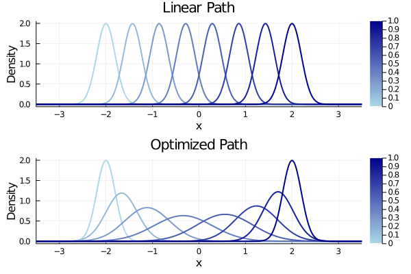
Figure 1: Two annealing paths between a $\pi_{0}=N(-2,0.2^{2})$ (light blue) and $\pi_{1}=N(2,0.2^{2})$ (dark blue) : the traditional linear path (top) and an optimized nonlinear path (bottom). While the distributions in the linear path are nearly mutually singular, those in the optimized path overlap substantially, leading to faster round trips.

Therefore, upon decreasing the variance of the reference and target while holding their means fixed, the traditional linear annealing path obtains an exponentially smaller asymptotic round trip rate than the optimal path of Gaussian distributions. Figure 1 provides an intuitive explanation. The standard path (top) corresponds to a set of Gaussian distributions with mean interpolated between the reference and target. If one reduces the variance of the reference and target, so does the variance of the distributions along the path. For any fixed $N$, these distributions become nearly mutually singular, leading to arbitrarily low round trip rates. The solution to this issue (bottom) is to allow the distributions along the path to have increased variances, thereby maintaining mutual overlap and the ability to swap components with a reasonable probability. This motivates the need to design more general annealing paths. In the following, we introduce the precise general definition of an annealing path, an analysis of path communication efficiency in parallel tempering, and a rigorous formulation of—and solution to—the problem of tuning path parameters to maximize communication efficiency.

3.1 Assumptions

Let $\mathcal{P}(\mathcal{X})$ be the set of probability densities with full support on a state space $\mathcal{X}$. For any collection of densities $\pi_{t}\in\mathcal{P}(\mathcal{X})$ with index $t\in[0,1]$, associate to each a log-density function $W_{t}$ such that

$$\pi_{t}(x)=\frac{1}{Z_{t}}\exp\left(W_{t}(x)\right),\quad x\in\mathcal{X},$$ (4)

where $Z_{t}=\int_{\mathcal{X}}\exp\left(W_{t}(x)\right)\textrm{d}x$ is the normalizing constant. Definition 1 provides the conditions necessary to form a path of distributions from a reference $\pi_{0}$ to a target $\pi_{1}$ that are well-behaved for use in parallel tempering.

Definition 1.

An annealing path is a map $\pi_{(\cdot)}:[0,1]\to\mathcal{P}(\mathcal{X})$, denoted $t\mapsto\pi_{t}$, such that for all $x\in\mathcal{X}$, $\pi_{t}(x)$ is continuous in $t$.

There are many ways to move beyond the standard linear path $\pi_{t}\propto\pi_{0}^{1-t}\pi_{1}^{t}$. For example, consider a nonlinear path $\pi_{t}\propto\pi_{0}^{\eta_{0}(t)}\pi_{1}^{\eta_{1}(t)}$ where $\eta_{i}:[0,1]\to{\mathbb{R}}$ are continuous functions such that $\eta_{0}(0)=\eta_{1}(1)=1$ and $\eta_{0}(1)=\eta_{1}(0)=0$. As long as for all $t\in[0,1]$, $\pi_{t}$ is a normalizable density this is a valid annealing path between $\pi_{0}$ and $\pi_{1}$. Further, note that the path parameter does not necessarily have to appear as an exponent: consider for example the mixture path $\pi_{t}\propto(1-t)\pi_{0}+t\pi$. Section 4 provides a more detailed example based on linear splines.

3.2 Communication efficiency analysis

Given a particular annealing path satisfying Definition 1, we require a method to characterize the round trip rate performance of parallel tempering based on that path. The results presented in this section form the basis of the objective function used to optimize over paths, as well as the foundation for the proof of Proposition 1.

We start with some notation for the rejection rates involved when Algorithm 1 is used with nonlinear paths (Equation 4). For $t,t^{\prime}\in[0,1]$, $x\in\mathcal{X}$, define the rejection rate function $r:[0,1]^{2}\to[0,1]$ to be

$$r(t,t^{\prime})=1-{\mathbb{E}}\left[\exp\left(\min\{0,A_{t,t^{\prime}}(X,X^{\prime})\}\right)\right]$$

$$A_{t,t^{\prime}}(x,x^{\prime})=(W_{t^{\prime}}(x)-W_{t}(x))-(W_{t^{\prime}}(x^{\prime})-W_{t}(x^{\prime})),$$

where $X\sim\pi_{t}$ and $X^{\prime}\sim\pi_{t^{\prime}}$ are independent. Assuming that all chains have reached stationarity, and all chains undergo efficient local exploration—i.e., $W_{t}(X),W_{t}(\tilde{X})$ are independent when $X\sim\pi_{t}$ and $\tilde{X}$ is generated by local exploration from $X$—then the round trip rate for a particular schedule $\mathcal{T}_{N}$ has the form given earlier in Equation (2). This statement follows from Syed et al. (2019, Cor. 1) without modification, because the proof of that result does not depend on the form of the acceptance ratio.

Our next objective is to characterize the asymptotic communication efficiency of a nonlinear path in the regime where $N\to\infty$ and $\|\mathcal{T}_{N}\|\to 0$—which establishes its fundamental ability to take advantage of parallel computation. In other words, we require a generalization of the asymptotic result in Equation (3). In this case, previous theory relies on the particular form of the acceptance ratio for linear paths (Syed et al., 2019); in the remainder of this section, we provide a generalization of the asymptotic result for nonlinear paths by piecewise approximation by a linear spline.

For $t,t^{\prime}\in[0,1]$, define $\Lambda(t,t^{\prime})$ to be the global communication barrier for the linear secant connecting $\pi_{t}$ and $\pi_{t}^{\prime}$,

$$\Lambda(t,t^{\prime}) =\frac{1}{2}\int_{0}^{1}{\mathbb{E}}[|A_{t,t^{\prime}}(X_{s},X^{\prime}_{s})|]{\mathrm{d}}s,$$ (5)

$$X_{s},X^{\prime}_{s} \overset{\text{i.i.d.}}{\sim}\frac{1}{Z_{s}(t,t^{\prime})}\exp\left((1-s)W_{t}+sW_{t^{\prime}}\right).$$

Lemma 1 shows that the global communication barrier $\Lambda(t,t^{\prime})$ along the secant of the path connecting $t$ to $t^{\prime}$ is a good approximation of the true rejection rate $r(t,t^{\prime})$ with $O(|t-t^{\prime}|^{3})$ error as $t\to t^{\prime}$.

Lemma 1.

Suppose that for all $x\in\mathcal{X}$, $W_{t}(x)$ is piecewise continuously differentiable in $t$, and that there exists $V_{1}:\mathcal{X}\to[0,\infty)$ such that

$$\forall x\in\mathcal{X},\,\,\sup_{t\in[0,1]}\left|\frac{{\mathrm{d}}W_{t}}{{\mathrm{d}}t}(x)\right|\leq V_{1}(x),$$ (6)

and

$$\sup_{t\in[0,1]}{\mathbb{E}}_{\pi_{t}}[V_{1}^{3}]<\infty.$$ (7)

Then there exists a constant $C<\infty$ independent of $t,t^{\prime}$ such that for all $t,t^{\prime}\in[0,1]$,

$$|r(t,t^{\prime})-\Lambda(t,t^{\prime})|\leq C|t-t^{\prime}|^{3}.$$ (8)

A direct consequence of Lemma 1 is that for any fixed schedule $\mathcal{T}_{N}$,

$$\left|\sum_{n=0}^{N-1}r(t_{n},t_{n+1})-\Lambda(\mathcal{T}_{N})\right|\leq C\|\mathcal{T}_{N}\|^{2},$$ (9)

where $\Lambda(\mathcal{T}_{N})=\sum_{n=0}^{N-1}\Lambda(t_{n},t_{n+1})$. Intuitively, in the $\|\mathcal{T}_{N}\|\approx 0$ regime where rejection rates are low,

$$\frac{r(t_{n},t_{n+1})}{1-r(t_{n},t_{n+1})}\approx r(t_{n},t_{n+1}),$$

and we have that $\tau(\mathcal{T}_{N})\approx(2+2\Lambda(\mathcal{T}_{N}))^{-1}$. Therefore, $\Lambda(\mathcal{T}_{N})$ characterizes the communication efficiency of the path in a way that naturally extends the global communication barrier from the linear path case. Theorem 2 provides the precise statement: the convergence is uniform in $\mathcal{T}_{N}$ and depends only on $\|\mathcal{T}_{N}\|$, and $\Lambda(\mathcal{T}_{N})$ itself converges to a constant $\Lambda$ in the asymptotic regime. We refer to $\Lambda$, defined below in Equation (13) as the global communication barrier for the general annealing path.

Theorem 2.

Suppose that for all $x\in\mathcal{X}$, $W_{t}(x)$ is piecewise twice continuously differentiable in $t$, that there exists $V_{1}:\mathcal{X}\to[0,\infty)$ satisfying (6) and (7), and that there exists $V_{2}:\mathcal{X}\to[0,\infty)$, $\epsilon>0$ satisfying

$$\forall x\in\mathcal{X},\,\,\sup_{t\in[0,1]}\left|\frac{{\mathrm{d}}^{2}W_{t}}{{\mathrm{d}}t^{2}}(x)\right|\leq V_{2}(x),$$ (10)

and

$$\sup_{t\in[0,1]}{\mathbb{E}}_{\pi_{t}}\left[(1+V_{1})\exp(\epsilon V_{2})\right]<\infty.$$ (11)

Then,

$$\lim_{\delta\to 0}\sup_{\mathcal{T}_{N}:\|\mathcal{T}_{N}\|\leq\delta}\left|(2+2\Lambda(\mathcal{T}_{N}))^{-1}-\tau(\mathcal{T}_{N})\right| =0$$ (12)

$$\text{and}\quad\lim_{\delta\to 0}\sup_{\mathcal{T}_{N}:\|\mathcal{T}_{N}\|\leq\delta}\left|\Lambda(\mathcal{T}_{N})-\Lambda\right| =0,$$ (13)

where $\Lambda=\int_{0}^{1}\lambda(t){\mathrm{d}}t$ for an instantaneous rejection rate function $\lambda:[0,1]\to[0,\infty)$ given by

$$\lambda(t) =\lim_{\Delta t\to 0}\frac{r(t+\Delta t,t)}{|\Delta t|}$$

$$=\frac{1}{2}{\mathbb{E}}\left[\left|\frac{dW_{t}}{dt}(X_{t})-\frac{dW_{t}}{dt}(X_{t}^{\prime})\right|\right],\quad X_{t},X^{\prime}_{t}\overset{\text{i.i.d.}}{\sim}\pi_{t}.$$

The integrability condition is required to control the tail behaviour of distributions formed by linearized approximations to the path $\pi_{t}$. This condition is satisfied by a wide range of annealing paths, e.g., the linear spline paths proposed in this work—since in that case $V_{2}=0$.

3.3 Annealing path families and optimization

It is often the case that there are a set of candidate annealing paths in consideration for a particular target $\pi$. For example, if a path has tunable parameters $\phi\in\Phi$ that govern its shape, we can generate a collection of annealing paths that all target $\pi$ by varying the parameter $\phi$. We call such collections an annealing path family.

Definition 3.

An annealing path family for target $\pi_{1}$ is a collection of annealing paths $\{\pi^{\phi}_{t}\}_{\phi\in\Phi}$ such that for all parameters $\phi\in\Phi$, $\pi^{\phi}_{1}=\pi_{1}$.

There are many ways to construct useful annealing path families. For example, if one is provided a parametric family of variational distributions $\{q_{\phi}:\phi\in\Phi\}$ for some parameter space $\Phi$, one can construct the annealing path family of linear paths $\pi^{\phi}_{t}=q_{\phi}^{1-t}\pi_{1}^{t}$ from a variational reference $q_{\phi}$ to the target $\pi_{1}$. More generally, given $\eta_{i}(t)$ satisfying the constraints in Section 3.1, $\pi^{\phi}_{t}=q_{\phi}^{\eta_{0}(t)}\pi_{1}^{\eta_{1}(t)}$ defines a nonlinear annealing path family. Another example of an annealing path family used in the context of PT are $q$-paths $\{\pi_{t}^{q}\}_{q\in[0,1]}$ (Whitfield et al., 2002). Given a fixed reference and target $\pi_{0},\pi_{1}$, the path $\pi_{t}^{q}$ interpolates between the mixture path ($q=0$) and the linear path ($q=1$) (Brekelmans et al., 2020). In Section 4, we provide a new flexible class of nonlinear paths based on splines that is designed specifically to enhance the performance of parallel tempering.

Since every path in an annealing path family has the desired target distribution $\pi_{1}$, we are free to optimize the path over the tuning parameter space $\phi\in\Phi$ in addition to optimizing the schedule $\mathcal{T}_{N}$. Motivated by the analysis of Section 3.2, a natural objective function for this optimization to consider is the non-asymptotic round trip rate

$$\phi^{\star},\mathcal{T}_{N}^{\star} =\operatornamewithlimits{arg\,max}_{\phi\in\Phi,\mathcal{T}_{N}}\,\tau^{\phi}(\mathcal{T}_{N})$$ (14)

$$=\operatornamewithlimits{arg\,min}_{\phi\in\Phi,\mathcal{T}_{N}}\sum_{n=0}^{N-1}\frac{r^{\phi}(t_{n},t_{n+1})}{1-r^{\phi}(t_{n},t_{n+1})},$$ (15)

where now the round trip rate and rejection rates depend both on the schedule and path parameter, denoted by superscript $\phi$. We solve this optimization using an approximate coordinate-descent procedure, iterating between an update of the schedule $\mathcal{T}_{N}$ for a fixed path parameter $\phi\in\Phi$, followed by a gradient step in $\phi$ based on a surrogate objective function and a fixed schedule. This is summarized in Algorithm 2. We outline the details of schedule and path tuning procedure in the following.

Algorithm 2 PathOptNRPT

0:  state x, path family $\pi^{\phi}_{t}$, parameter $\phi$, # chains $N$, # PT iterations $M$, # tuning steps $S$, learning rate $\gamma$

  $\mathcal{T}_{N}\leftarrow(0,1/N,2/N,\dots,1)$

  for $s=1$ to $S$ do

     $\{\textbf{x}_{m}\}_{m=1}^{M},(r_{n})_{n=0}^{N}\leftarrow\texttt{NRPT}(\textbf{x},\pi^{\phi}_{t},\mathcal{T}_{N},M)$

     $\lambda^{\phi}\leftarrow\texttt{CommunicationBarrier}(\mathcal{T}_{N},\{r_{n}\})$

     $\mathcal{T}_{N}\leftarrow\texttt{UpdateSchedule}(\lambda^{\phi},N)$

     $\phi\leftarrow\phi-\gamma\nabla_{\phi}\sum_{n=0}^{N-1}\mathrm{SKL}(\pi^{\phi}_{t_{n}},\pi^{\phi}_{t_{n+1}})$

     $\textbf{x}\leftarrow\textbf{x}_{M}$

  end for

  Return: $\phi,\mathcal{T}_{N}$

Tuning the schedule

Fix the value of $\phi$, which fixes the path. We adapt a schedule tuning algorithm from past work to update the schedule $\mathcal{T}_{N}=(t_{n})_{n=0}^{N}$ (Syed et al., 2019, Section 5.1). Based on the same argument as this previous work, we obtain that when $\|\mathcal{T}_{N}\|\approx 0$, the non-asymptotic round trip rate is maximized when the rejection rates are all equal. The schedule that approximately achieves this satisfies

$$\forall n\in\{1,\dots,N-1\},\quad\frac{1}{\Lambda^{\phi}}\int_{0}^{t_{n}}\lambda^{\phi}(s){\mathrm{d}}s=\frac{n}{N}.$$ (16)

Following Syed et al. (2019), we use Monte Carlo estimates of the rejection rates $r^{\phi}(t_{n},t_{n+1})$ to approximate $t\mapsto\int_{0}^{t}\lambda^{\phi}(s)\textrm{d}s$, $s\in[0,1]$ via a monotone cubic spline, and then use bisection search to solve for each $t_{n}$ according to Equation (16).

Optimizing the path

Fix the schedule $\mathcal{T}_{N}$; we now want to improve the path itself by modifying $\phi$. However, in challenging problems this is not as simple as taking a gradient step for the objective in Equation (14). In particular, in early iterations—when the path is near its oft-poor initialization—the rejection rates satisfy $r^{\phi}(t_{n},t_{n+1})\approx 1$. As demonstrated empirically in Appendix F, gradient estimates in this regime exhibit a low signal-to-noise ratio that precludes their use for optimization.

We propose a surrogate, the symmetric KL divergence, motivated as follows. Consider first the global communication barrier $\Lambda^{\phi}(\mathcal{T}_{N})$ for the linear spline approximation to the path; Theorem 2 guarantees that as long as $\|\mathcal{T}_{N}\|$ is small enough, one can optimize $\Lambda^{\phi}(\mathcal{T}_{N})$ in place of the round trip rate $\tau^{\phi}(\mathcal{T}_{N})$. By Jensen’s inequality,

$$\frac{1}{N^{2}}\Lambda^{\phi}(\mathcal{T}_{N})^{2}\leq\frac{1}{N}\sum_{n=0}^{N-1}\Lambda^{\phi}(t_{n},t_{n+1})^{2}.$$

Next, we apply Jensen’s inequality again to the definition of $\Lambda^{\phi}(t_{n},t_{n+1})$ from (5), which shows that

$$\Lambda^{\phi}(t_{n},t_{n+1}))^{2}\leq\frac{1}{4}\int_{0}^{1}{\mathbb{E}}[A_{t_{n},t_{n+1}}(X_{s},X^{\prime}_{s})^{2}]{\mathrm{d}}s,$$

where $X_{s}$ are defined in (5) are drawn from the linear path between $\pi^{\phi}_{t_{n}}$ and $\pi^{\phi}_{t_{n+1}}$. Finally, we note that the inner expectation is the path integral of the Fisher information metric along the linear path and evaluates to the symmetric KL divergence (Dabak & Johnson, 2002, Result 4),

$$\int_{0}^{1}{\mathbb{E}}\left[(A_{t_{n},t_{n+1}}(X_{s},X^{\prime}_{s}))^{2}\right]{\mathrm{d}}s=2\mathrm{SKL}(\pi^{\phi}_{t_{n}},\pi^{\phi}_{t_{n+1}}).$$

Therefore we have

$$\frac{2\Lambda^{\phi}(\mathcal{T}_{N})^{2}}{N}\leq\sum_{n=0}^{N-1}\mathrm{SKL}(\pi^{\phi}_{t_{n}},\pi^{\phi}_{t_{n+1}}).$$ (17)

The slack in the inequality in Equation (17) could potentially depend on $\phi$ even in the large $N$ regime. Therefore, during optimization, we recommend monitoring the value of the original objective function (Equation (14)) to ensure that the optimization of the surrogate SKL objective indeed improves it, and hence the round trip rate performance of PT via Equation (2). In the experiments we display the values of both objective functions.

4 Spline annealing path family

In this section, we develop a family of annealing paths—the spline annealing path family—that offers a practical and flexible improvement upon the traditional linear paths considered in past work. We first define a general family of annealing paths based on the exponential family, and then provide the specific details of the spline family with a discussion of its properties. Empirical results in Section 5 demonstrate that the spline annealing path family resolves the problematic Gaussian annealing example in Figure 1.

4.1 Exponential annealing path family

We begin with the practical desiderata for an annealing path family given a fixed reference $\pi_{0}$ and target $\pi_{1}$ distribution. First, the traditional linear path $\pi_{t}\propto\pi_{0}^{1-t}\pi_{1}^{t}$ should be a member of the family, so that one can achieve at least the round trip rate provided by that path. Second, the family should be broadly applicable and not depend on particular details of either $\pi_{0}$ or $\pi_{1}$. Finally, using the Gaussian example from Figure 1 and Proposition 1 as insight, the family should enable the path to smoothly vary from $\pi_{0}$ to $\pi_{1}$ while inflating / deflating the variance as necessary.

These desiderata motivate the design of the exponential annealing path family, in which each annealing path takes the form

$$\pi_{t}\propto\pi_{0}^{\eta_{0}(t)}\pi_{1}^{\eta_{1}(t)}=\exp(\eta(t)^{T}W(x)),$$

for some function $\eta(t)=(\eta_{0}(t),\eta_{1}(t))$ and reference/target log densities $W(x)=(W_{0}(x),W_{1}(x))$. Intuitively, $\eta_{0}(t)$ and $\eta_{1}(t)$ represent the level of annealing for the reference and target respectively along the path. Proposition 2 shows that a broad collection of functions $\eta$ indeed construct a valid annealing path family including the linear path.

Proposition 2.

Let $\Omega\subseteq{\mathbb{R}}^{2}$ be the set

$$\Omega\!=\!\left\{\xi\in{\mathbb{R}}^{2}\!:\!\!\int\exp(\xi^{T}W(x)){\mathrm{d}}x<\infty\right\}.$$

Suppose $(0,1)\in\Omega$ and $\mathcal{A}$ is a set of piecewise twice continuously differentiable functions $\eta:[0,1]\to\Omega$ such that $\eta(1)=(0,1)$. Then

$$\left\{\pi_{t}(x)\propto\exp(\eta(t)^{T}W(x)):\eta\in\mathcal{A}\right\}$$

is an annealing path family for target distribution $\pi_{1}$. If additionally $(1,0)\in\Omega$, then the linear path $\eta(t)=(1-t,t)$ may be included in $\mathcal{A}$. Finally, if for every $\eta\in\mathcal{A}$ there exists $M>0$ such that $\sup_{t}\max\{\|\eta^{\prime}(t)\|_{2},\|\eta^{\prime\prime}(t)\|_{2}\}\leq M$ and Equation (11) holds with $V_{1}=V_{2}=M\|W\|_{2}$, then each path in the family satisfies the conditions of Theorem 2.

4.2 Spline annealing path family

Proposition 2 reduces the problem of designing a general family of paths of probability distributions to the much simpler task of designing paths in ${\mathbb{R}}^{2}$. We argue that a good choice can be constructed using linear spline paths connecting $K$ knots $\phi=(\phi_{0},\dots,\phi_{K})\in({\mathbb{R}}^{2})^{K+1}$, i.e., for all $k\in\{1,\dots,K\}$ and $t\in[\frac{k-1}{K},\frac{k}{K}]$,

$$\eta^{\phi}(t)\mapsto(k-Kt)\phi_{k-1}+(Kt-k+1)\phi_{k}.$$

Let $\Omega$ be defined as in Proposition 2. The $K$-knot spline annealing path family is defined as the set of $K$-knot linear spline paths such that

$$\phi_{0}=(1,0),\quad\phi_{K}=(0,1),\quad\text{and}\quad\forall k,\,\,\phi_{k}\in\Omega.$$

Validity:

Since $\Omega$ is a convex set per the proof of Proposition 2, we are guaranteed that $\eta^{\phi}([0,1])\subseteq\Omega$, and so this collection of annealing paths is a subset of the exponential annealing family and hence forms a valid annealing path family targeting $\pi_{1}$.

Convexity:

Furthermore, convexity of $\Omega$ implies that tuning the knots $\phi\in\Omega^{K+1}$ involves optimization within a convex constraint set. In practice, we enforce also that the knots are monotone in each component—i.e., the first component monotonically decreases, $1=\phi_{0,0}\geq\phi_{1,0}\geq\dots\geq\phi_{K,0}=0$ and the second increases, $0=\phi_{0,1}\leq\phi_{1,1}\leq\dots\leq\phi_{K,1}=1$ —such that the path of distributions always moves from the reference to the target. Because monotonicity constraint sets are linear and hence convex, the overall monotonicity-constrained optimization problem has a convex domain.

Flexibility:

Assuming the family is nonempty, it trivially contains the linear path. Further, given a large enough number of knots $K$, the spline annealing family well-approximates subsets of the exponential annealing family for fixed $M>0$. In particular,

$$\sup_{\eta\in\mathcal{A}_{M}}\inf_{\phi\in\Omega^{K+1}}\|\eta^{\phi}-\eta\|_{\infty}\leq\frac{M}{4K^{2}}.$$ (18)

Figure 2 provides an illustration of the behaviour of optimized spline paths for a Gaussian reference and target. The path takes a convex curved shape; starting at the bottom right point of the figure (reference), this path corresponds to increasing the variance of the reference, shifting the mean from reference to target, and finally decreasing the variance to match the target. With more knots, this process happens more smoothly.

Appendix D provides an explicit derivation of the stochastic gradient estimates we use to optimize the knots of the spline annealing path family. It is also worth making two practical notes. First, to enforce the monotonicity constraint, we developed an alternative to the usual projection approach, as projecting into the set of monotone splines can cause several knots to become superposed. Instead, we maintain monotonicity as follows: after each stochastic gradient step, we identify a monotone subsequence of knots containing the endpoints, remove the nonmonotone jumps, and linearly interpolate between the knot subsequence with an even spacing. Second, we take gradient steps in a log-transformed space so that knot components are always strictly positive.

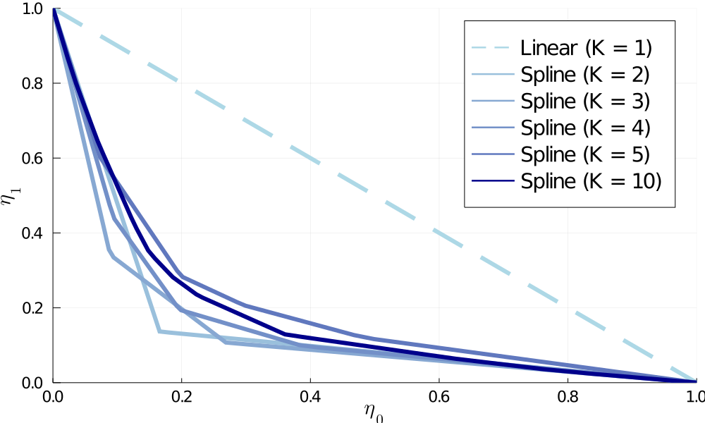
Figure 2: The spline path for $K=1,2,3,4,5,10$ knots for the family generated by $\pi_{0}=N(-1,0.5)$ and $\pi_{1}=N(1,0.5)$.

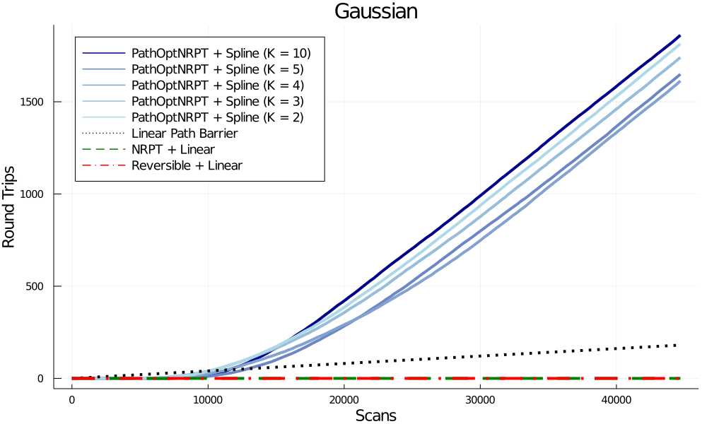
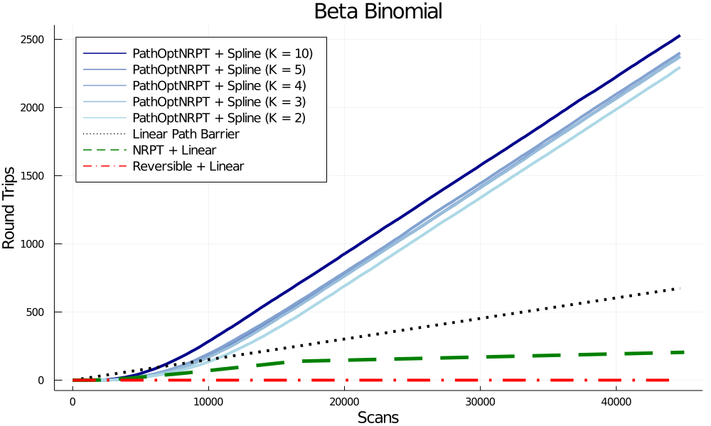
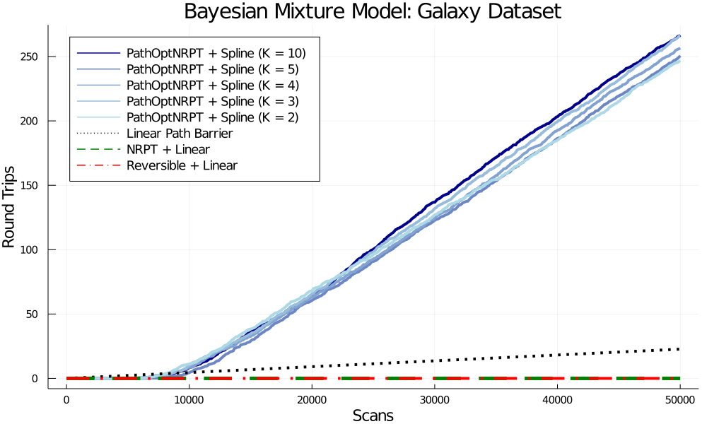
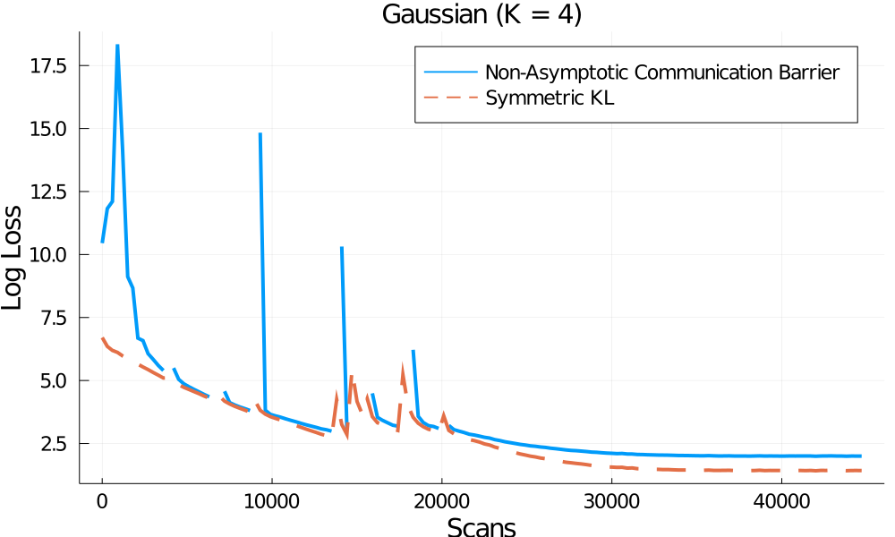
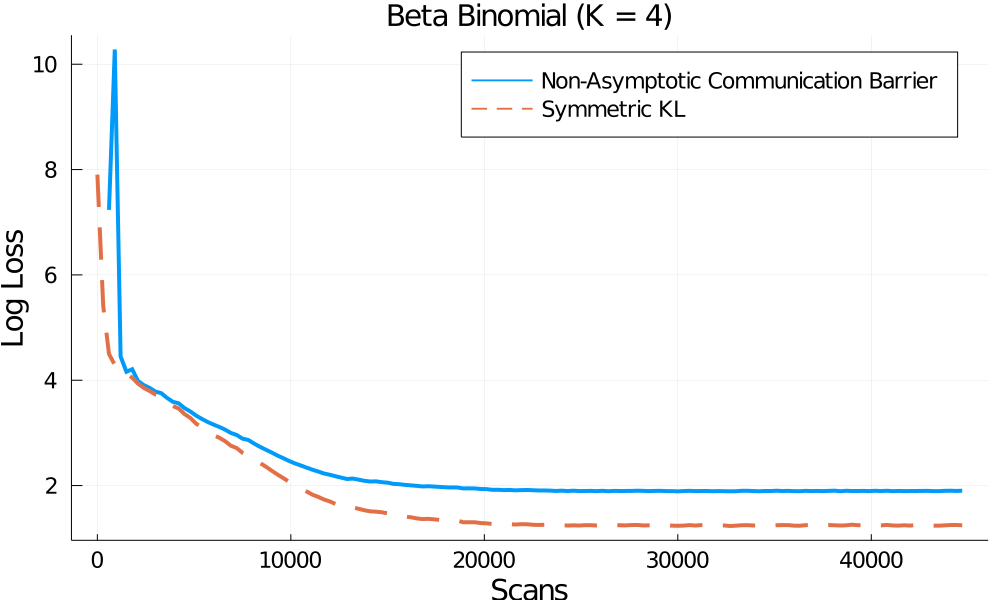
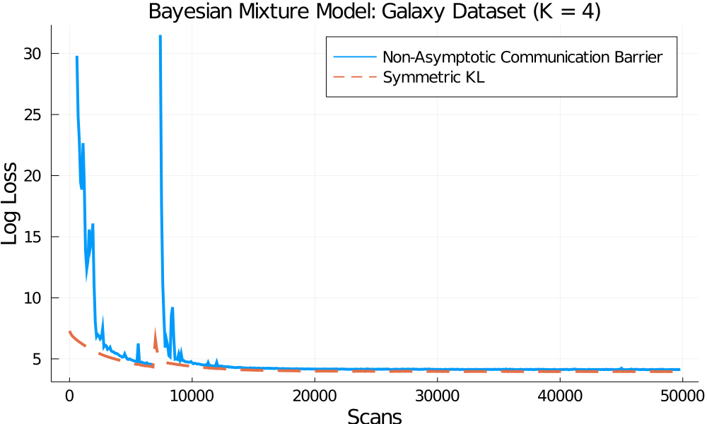
Figure 3: Top: Cumulative round trips averaged over 10 runs for the spline path with $K=2,3,4,5,10$ (solid blue), NRPT using a linear path (dashed green), and reversible PT with linear path (dash/dot red). The slope of the lines represent the round trip rate. We observe large gains going from linear to non-linear paths ($K>1$). For all values of $K>1$, the optimized spline path substantially improves on the theoretical upper bound on round trip rate possible using linear path (dotted black). Bottom: Non-asymptotic communication barrier from Equation 15 (solid blue) and Symmetric KL (dash orange) as a function of iteration for one run of PathOptNRPT + Spline ($K=4$ knots).

5 Experiments

In this section, we study the empirical performance of non-reversible PT based on the spline annealing path family ($K\in\{2,3,4,5,10\}$) from Section 4, with knots and schedule optimized using the tuning method from Section 3. We compare this method to two PT methods based on standard linear paths: non-reversible PT with adaptive schedule (“NRPT+Linear”) (Syed et al., 2019), and reversible PT (“Reversible+Linear”) (Atchadé et al., 2011). Code for the experiments is available at https://github.com/vittrom/PT-pathoptim.

We use the terminology “scan” to denote one iteration of the for loop in Algorithm 2. The computational cost of a scan is comparable for all the methods, since the bottleneck is the local exploration step shared by all methods. These experiments demonstrate two primary conclusions: (1) tuned nonlinear paths provide a substantially higher round trip rate compared to linear paths for the examples considered; and (2) the symmetric KL sum objective (Equation 17) is a good proxy for the round trip rate as a tuning objective.

We run the following benchmark problems; see the supplement for details. Gaussian: a synthetic setup in which the reference distribution is $\pi_{0}=N(-1,0.01^{2})$ and the target is $\pi_{1}=N(1,0.01^{2})$. For this example we used $N=50$ parallel chains and fixed the computational budget to 45000 samples. For Algorithm 2, the computational budget was divided equally over 150 scans, meaning 300 samples were used for every gradient update. “Reversible+Linear” performed 45000 local exploration steps with a communication step after every iteration while for “NRPT+Linear” the computational budget was used to adapt the schedule. The gradient updates were performed using Adagrad (Duchi et al., 2011) with learning rate equal to 0.2. Beta-binomial model: a conjugate Bayesian model with prior $\pi_{0}(p)=\mathrm{Beta}(180,840)$ and likelihood $L(x|p)=\mathrm{Binomial}(x|n,p)$. We simulated data $x_{1},\dots,x_{2000}\sim\mathrm{Binomial}(100,0.7)$ resulting in a posterior $\pi_{1}(p)=\mathrm{Beta}(140180,60840)$. The prior and posterior are heavily concentrated at 0.2 and 0.7 respectively. We used the same settings as for the Gaussian example. Galaxy data: A Bayesian Gaussian mixture model applied to the galaxy dataset of (Roeder, 1990). We used six mixture components with mixture proportions $w_{0},\ldots,w_{5}$, mixture component densities $N(\mu_{i},1)$ for mean parameters $\mu_{0},\ldots,\mu_{5}$, and a cluster label categorical variable for each data point. We placed a $\mathrm{Dir}(\boldsymbol{1}_{6})$ prior on the proportions, where $\boldsymbol{1}_{6}=(1,1,1,1,1,1)$ and a $N(150,1)$ prior on each of the mean parameters. We did not marginalize the cluster indicators, creating a multi-modal posterior inference problem over 94 latent variables. In this experiment we used $N=35$ chains and fixed the computational budget to 50000 samples, divided into 500 scans using 100 samples each. We optimized the path using Adagrad with a learning rate of 0.3. Exploring the full posterior distribution is challenging in this context due to a combination of misspecification of the prior and label switching. Label switching refers to the invariance of the likelihood under relabelling of the cluster labels. In Bayesian problems label switching can lead to increased difficulty of the sampling problem as it generates symmetric multi-modal posterior distributions. High dimensional Gaussian: a similar setup to the one-dimensional Gaussian experiment where the number of dimensions ranges from $d=1$ to $d=256$. The reference distribution is $\pi_{0}=N(-\boldsymbol{1}_{d},(0.1^{2})I_{d})$ and the target is $\pi_{1}=N(\boldsymbol{1}_{d},(0.1^{2})I_{d})$ where the subscript $d$ indicates the dimensionality of the problem. The number of chains $N$ is set to increase with dimension at the rate $N=\lceil 15\sqrt{d}\rceil$. We fixed the number of spline knots $K$ to 4 and set the computational budget to 50000 samples divided into 500 scans with 100 samples per gradient update. The gradient updates were performed using Adagrad with learning rate equal to 0.2. For all the experiments we performed one local exploration step before each communication step.

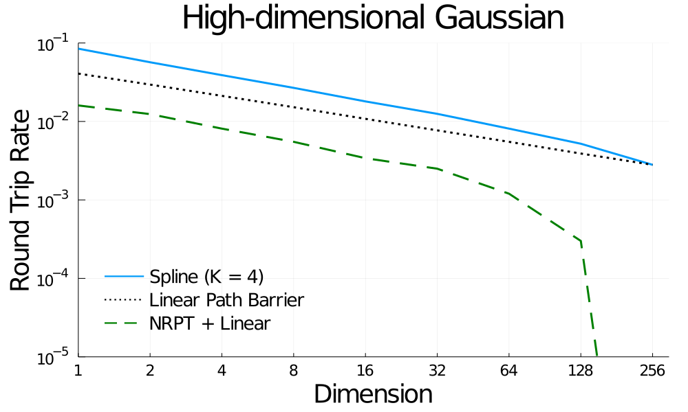
Figure 4: Round trips rate averaged over 5 runs for the spline path with $K=4$ (solid blue), NRPT using a linear path (dashed green) and theoretical upper bound on round trip rate possible using linear path (dotted black) as a function of the dimensionality of the target distribution.

The results of these experiments are shown in Figures 3 and 4. Examining the top row of Figure 3—which shows the number of round trips as a function of the number of scans—one can see that PT using the spline annealing family outperforms PT using the linear annealing path across all numbers of knots tested. Moreover, the slope of these curves demonstrates that PT with the spline annealing family exceeds the theoretical upper bound of round trip rate for the linear annealing path (from Equation (12)). The largest gain is obtained from going from $K=1$ (linear) to $K=2$. For all the examples, increasing the number of knots to more than $K>2$ leads to marginal improvements. In the case of the Gaussian example, note that since the global communication barrier $\Lambda$ for the linear path is much larger than $N$, algorithms based on linear paths incurred rejection rates of nearly one for most chains, resulting in no round trips.

The bottom row of Figure 3 shows the value of the surrogate SKL objective and non-asymptotic communication barrier from Equation (15). In particular, these figures demonstrate that the SKL provides a surrogate objective that is a reasonable proxy for the non-asymptotic communication barrier, but does not exhibit as large estimation variance in early iterations when there are pairs of chains with rejection rates close to one.

Figure 4 shows the round trip rate as a function of the dimensionality of the problem for Gaussian target distributions. As the dimensionality increases, the sampling problem becomes fundamentally more difficult, explaining the decay in performance of both NRPT with a linear path and an optimized path. Both sampling methods are provided with a fixed computational budget in all runs. Due to this fixed budget, NRPT is unable for $d\geq 64$ to approach the optimal schedule in the alloted time. This leads to an increasing gap between the round trip rates of NRPT with linear path and the spline path for $d\geq 64$.

6 Discussion

In this work, we identified the use of linear paths of distributions as a major bottleneck in the performance of parallel tempering algorithms. To address this limitation, we have provided a theory of parallel tempering on nonlinear paths, a methodology to tune parametrized paths, and finally a practical, flexible family of paths based on linear splines. Future work in this line of research includes extensions to estimate normalization constants, as well as the development of techniques and theory surrounding the use of variational reference distributions.

Appendix A Proof of Proposition 1

Define $\pi_{0}=N(\mu_{0},\sigma^{2})$ and $\pi_{1}=N(\mu_{1},\sigma^{2})$ with $W_{i}(x)\propto-\frac{1}{2\sigma^{2}}(x-\mu_{i})^{2}$ (throughout we use the proportionality symbol $\propto$ with log-densities to indicate an unspecified constant, additive with respect to $W_{i}$, multiplicative with respect to $\pi_{t}$). Suppose $\pi_{t}$ is the linear path $\pi_{t}(x)\propto\exp(W_{t})$ where $W_{t}=(1-t)W_{0}+tW_{1}$. Note that as a function of $x$,

$$W_{t}(x) \propto-\frac{1-t}{2\sigma^{2}}(x-\mu_{0})^{2}-\frac{t}{2\sigma^{2}}(x-\mu_{1})^{2}$$

$$\propto-\frac{1}{2\sigma^{2}}(x-\mu_{t})^{2},\quad\mu_{t}=(1-t)\mu_{0}+t\mu_{1},$$

and thus $\pi_{t}=N(\mu_{t},\sigma^{2})$. Taking a derivative of $W_{t}$, we find that

$$\frac{{\mathrm{d}}W_{t}}{{\mathrm{d}}t}=\frac{(\mu_{1}-\mu_{0})\left(x-\frac{\mu_{0}+\mu_{1}}{2}\right)}{\sigma^{2}}.$$

We will now compute $\lambda(t)$. If $X_{t},X^{\prime}_{t}\sim\pi_{t}$, then

$$\lambda(t) =\frac{1}{2}{\mathbb{E}}\left[\left|\frac{dW}{dt}(X_{t})-\frac{dW}{dt}(X^{\prime}_{t})\right|\right]$$

$$=\frac{|\mu_{1}-\mu_{0}|}{2\sigma}{\mathbb{E}}\left[\left|\frac{X_{t}-\frac{\mu_{0}+\mu_{1}}{2}}{\sigma}-\frac{X_{t}^{\prime}-\frac{\mu_{0}+\mu_{1}}{2}}{\sigma}\right|\right]$$

$$=\frac{|\mu_{1}-\mu_{0}|}{2\sigma}{\mathbb{E}}\left[\left|\frac{X_{t}-\mu_{t}}{\sigma}-\frac{X_{t}^{\prime}-\mu_{t}}{\sigma}\right|\right]$$

$$=\frac{|\mu_{1}-\mu_{0}|}{2\sigma}{\mathbb{E}}\left[\left|Z-Z^{\prime}\right|\right],$$

where $Z,Z^{\prime}\sim N(0,1)$. Thus $Z-Z^{\prime}\sim N(0,2)$, and $|Z-Z^{\prime}|$ has a folded normal distribution with expectation $2/\sqrt{\pi}$. This implies $\lambda(t)=z/\sqrt{\pi}$ where $z=|\mu_{1}-\mu_{0}|/\sigma$ and $\Lambda=\int_{0}^{1}\lambda(t){\mathrm{d}}t=z/\sqrt{\pi}$. By Theorem 2, the asymptotic round trip rate $\tau_{\infty}^{\mathrm{linear}}$ for the linear path satisfies,

$$\tau_{\infty}^{\mathrm{linear}}=\frac{1}{2+2\Lambda}=\frac{1}{2+2z/\sqrt{\pi}}=\Theta\left(\frac{1}{z}\right).$$

We will now establish an upper bound for the communication barrier $\Lambda$ for a general path $\pi_{t}$. If $X_{t},X_{t}^{\prime}\sim\pi_{t}$, then Theorem 2 and Jensen’s inequality imply the following:

$$\Lambda =\int_{0}^{1}\frac{1}{2}{\mathbb{E}}\left[\sqrt{\left(\frac{dW}{dt}(X_{t})-\frac{dW}{dt}(X^{\prime}_{t})\right)^{2}}\right]{\mathrm{d}}t$$

$$\leq\int_{0}^{1}\frac{1}{2}\sqrt{{\mathbb{E}}\left[\left(\frac{dW}{dt}(X_{t})-\frac{dW}{dt}(X^{\prime}_{t})\right)^{2}\right]}{\mathrm{d}}t$$

$$=\frac{1}{\sqrt{2}}\int_{0}^{1}\sqrt{\mathrm{Var}_{\pi_{t}}\left[\frac{dW_{t}}{dt}\right]}{\mathrm{d}}t$$

$$=\frac{1}{\sqrt{2}}\Lambda_{F},$$

where $\Lambda_{F}$ is the length of the the path $\pi_{t}$ with the Fisher information metric. The geodesic path of Gaussians between $\pi_{0}$ and $\pi_{1}$ that minimizes $\Lambda_{F}$ satisfies (Costa et al., 2015, Eq. 11, Sec. 2)

$$\Lambda_{F}=\sqrt{2}\log\left(1+\frac{z^{2}}{4}+\frac{z}{4}\sqrt{8+z^{2}}\right).$$ (19)

Again, by Theorem 2, the asymptotic round trip rate $\tau_{\infty}^{\mathrm{geodesic}}$ for the geodesic path satisfies

$$\tau_{\infty}^{\mathrm{geodesic}}=\frac{1}{2+2\Lambda}\geq\frac{1}{2+2\Lambda_{F}}=\Theta\left(\frac{1}{\log z}\right).$$

Appendix B Proof of Lemma 1

Definition 4.

Given a path $\pi_{t}$ and measurable function $f$, we denote $\|f\|_{\pi}=\sup_{t}{\mathbb{E}}_{\pi_{t}}[f]$.

Following the computation in Predescu et al. (2004, Equation (6)), we have

$$r(t,t^{\prime})=1-\frac{{\mathbb{E}}[\exp(-\frac{1}{2}|A_{t,t^{\prime}}(\tilde{X}_{1/2},\tilde{X}^{\prime}_{1/2})|]}{{\mathbb{E}}[\exp(-\frac{1}{2}A_{t,t^{\prime}}(\tilde{X}_{1/2},\tilde{X}^{\prime}_{1/2}))]},$$ (20)

where $\tilde{X}_{s},\tilde{X}^{\prime}_{s}\sim\tilde{\pi}_{s}=\frac{1}{\tilde{Z}(s)}\exp((1-s)W_{t}+sW_{t^{\prime}})$ and

$$A_{t,t^{\prime}}(x,x^{\prime})=(W_{t^{\prime}}(x)-W_{t}(x))-(W_{t^{\prime}}(x^{\prime})-W_{t}(x^{\prime})).$$

In particular, the path of distributions $\tilde{\pi}_{s}$ for $s\in[0,1]$ is the linear path between $\pi_{t}$ and $\pi_{t^{\prime}}$.

Lemma 2.

Suppose (6) and (7) hold. Then for all $k\leq 3$, there is a constant $\tilde{C}_{k}$ independent of $t,t^{\prime},\mathcal{T}_{N}$ such that

$$\sup_{s}{\mathbb{E}}[|A_{t,t^{\prime}}(\tilde{X}_{s},\tilde{X}^{\prime}_{s})|^{k}]\leq\tilde{C}_{k}|t^{\prime}-t|^{k}.$$

where $\tilde{X}_{s},\tilde{X}_{s}^{\prime}\sim\tilde{\pi}_{s}$.

Proof.

The mean-value theorem and (6) imply that $W_{t}(x)$ is Lipschitz in $t$,

$$|W_{t}(x)-W_{t^{\prime}}(x)|\leq V_{1}(x)|t^{\prime}-t|.$$

The triangle inequality therefore implies

$$|A_{t,t^{\prime}}(x,x^{\prime})|\leq(V_{1}(x)+V_{1}(x^{\prime}))|t^{\prime}-t|.$$

By taking expectations and using the fact $|a+b|^{k}\leq 2^{k-1}(|a|^{k}+|b|^{k})$, we have that

$${\mathbb{E}}[|A_{t,t^{\prime}}(\tilde{X}_{s},\tilde{X}^{\prime}_{s})|^{k}] \leq 2^{k}{\mathbb{E}}_{\tilde{\pi}_{s}}[V_{1}^{k}]|t^{\prime}-t|^{k}$$

$$\leq 2^{k}{\mathbb{E}}_{\tilde{\pi}_{s}}[V_{1}^{3}]|t^{\prime}-t|^{k},$$

where in the last line we use the fact that we can assume $V_{1}\geq 1$ without loss of generality. The result follows by taking the supremum on both sides and noting that $\tilde{C}_{k}=2^{k}\|V_{1}^{3}\|_{\tilde{\pi}}$ is finite by (7). ∎

We now begin the proof of Lemma 1. Define $\tilde{\lambda}(s)=\frac{1}{2}{\mathbb{E}}[|A_{t,t^{\prime}}(\tilde{X}_{s},\tilde{X}^{\prime}_{s})|]$ for $\tilde{X}_{s},\tilde{X}^{\prime}_{s}\sim\tilde{\pi}_{s}$. Then a third order Taylor expansion of Equation (20) (Predescu et al., 2004), which contains terms of the form ${\mathbb{E}}[|A_{t,t^{\prime}}(\tilde{X}_{s},\tilde{X}^{\prime}_{s})|^{k}]$ that can be controlled via Lemma 2, yields

$$r(t,t^{\prime}) =\tilde{\lambda}(1/2)+R(t,t^{\prime}),\quad|R(t,t^{\prime})|\leq C^{\prime}|t-t^{\prime}|^{3},$$

for some finite constant $C^{\prime}$ independent of $t,t^{\prime}$. By Syed et al. (2019, Prop. 2, Appendix C) we have that in addition, $\tilde{\lambda}(s)$ is in $C^{2}([0,1])$, and thus there is a constant $C^{\prime\prime}$ independent of $t,t^{\prime}$ such that

$$\sup_{s}\left|\frac{d^{2}\tilde{\lambda}}{ds^{2}}\right|\leq C^{\prime\prime}|t-t^{\prime}|^{3}.$$

The error bound for the midpoint rule implies,

$$\left|\tilde{\lambda}(1/2)-\int_{0}^{1}\tilde{\lambda}(s)ds\right| \leq\frac{1}{24}\sup_{s}\left|\frac{d^{2}\tilde{\lambda}}{ds^{2}}\right|$$

$$\leq\frac{C^{\prime\prime}}{24}|t-t^{\prime}|^{3}.$$

The result follows: there is a finite constant $C$ independent of $t,t^{\prime}$ such that

$$\left|r(t,t^{\prime})-\Lambda(t,t^{\prime})\right|=\left|r(t,t^{\prime})-\int_{0}^{1}\tilde{\lambda}(s)ds\right|\leq C|t^{\prime}-t|^{3}.$$

Appendix C Proof of Theorem 2

We first note that without loss of generality we can place an artificial schedule point $t_{n}$ at each of the finitely many discontinuities in $W_{t}$ or its first/second derivative. Thus we assume the $W_{t}$ is $C^{2}$ on each interval $[t_{n-1},t_{n}]$. Later in the proof it will become clear that the contributions of these artificial schedule points becomes negligible as $\|\mathcal{T}_{N}\|\to 0$.

Given a schedule $\mathcal{T}_{N}$, define the path $\tilde{\pi}_{t}=\frac{1}{\tilde{Z}_{t}}\exp(\tilde{W}_{t})$ with log-likelihood $\tilde{W}_{t}$ satisfying for each segment $t_{n-1}\leq t\leq t_{n}$,

$$\tilde{W}_{t}=W_{t_{n-1}}+\frac{\Delta W_{n}}{\Delta t_{n}}(t-t_{n-1}),$$

where $\Delta W_{n}=W_{t_{n}}-W_{t_{n-1}}$ and $\Delta t_{n}=t_{n}-t_{n-1}$. In particular, $\tilde{W}_{t}$ agrees with $W_{t}$ for $t\in\mathcal{T}_{N}$, linearly interpolates between $W_{t_{n-1}}$ and $W_{t_{n}}$ for $t\in[t_{n-1},t_{n}]$, and for all $x$, from Taylor’s theorem:

$$|\tilde{W}_{t}(x)-W_{t}(x)|\leq\frac{1}{2}\sup_{t\in[t_{n-1},t_{n}]}\left|\frac{d^{2}W_{t}}{dt^{2}}(x)\right|\Delta t_{n}^{2}.$$ (21)

The following lemma shows that the normalization constant of, and expectations under, $\tilde{\pi}_{t}$ are comparable to the same for $\pi_{t}$ with an error bound that depends on $\|\mathcal{T}_{N}\|$ and converges to 0 as $\|\mathcal{T}_{N}\|\to 0$.

Lemma 3.

For measurable functions $f$ and $s>0$, let

$$E_{t}(f,s)={\mathbb{E}}_{\pi_{t}}\left[|f|e^{s^{2}V_{2}}\right],$$

and define $E_{t}(s)=E_{t}(1,s)$ for brevity.

1. For any schedule $\mathcal{T}_{N}$,

   $$\left|\frac{\tilde{Z}_{t}}{Z_{t}}-1\right|\leq E_{t}(\|\mathcal{T}_{N}\|)-1,$$

   and if $\|\mathcal{T}_{N}\|$ is small enough that $E_{t}(\|\mathcal{T}_{N}\|)<2$,

   $$\left|\frac{Z_{t}}{\tilde{Z}_{t}}-1\right|\leq\frac{E_{t}(\|\mathcal{T}_{N}\|)-1}{2-E_{t}(\|\mathcal{T}_{N}\|)}.$$

2. For any schedule $\mathcal{T}_{N}$ and measureable function $f$, if $\|\mathcal{T}_{N}\|$ is small enough that $E_{t}(\|\mathcal{T}_{N}\|)<2$,

   $$\left|{\mathbb{E}}_{\tilde{\pi}_{t}}[f]-{\mathbb{E}}_{\pi_{t}}[f]\right| \leq\frac{E_{t}(\|\mathcal{T}_{N}\|)-1}{2-E_{t}(\|\mathcal{T}_{N}\|)}E_{t}(f,\|\mathcal{T}_{N}\|)$$

   $$+E_{t}(f,\|\mathcal{T}_{N}\|)-E_{t}(f,0).$$

Proof.

1. We rewrite the expression

   $$\frac{\tilde{Z}_{t}}{Z_{t}} =\frac{1}{Z_{t}}\int_{\mathcal{X}}e^{\tilde{W}_{t}(x)}{\mathrm{d}}x$$

   $$=\int_{\mathcal{X}}e^{\tilde{W}_{t}(x)-W_{t}(x)}\pi_{t}(x){\mathrm{d}}x$$

   $$=1+\int_{\mathcal{X}}\left(e^{\tilde{W}_{t}(x)-W_{t}(x)}-1\right)\pi_{t}(x){\mathrm{d}}x.$$

   Thus using the inequality $|e^{x}-1|\leq e^{|x|}-1$,

   $$\left|\frac{\tilde{Z}_{t}}{Z_{t}}-1\right| \leq\left|\int_{\mathcal{X}}\left(e^{\tilde{W}_{t}(x)-W_{t}(x)}-1\right)\pi_{t}(x){\mathrm{d}}x\right|$$

   $$\leq\int_{\mathcal{X}}\left(e^{|\tilde{W}_{t}(x)-W_{t}(x)|}-1\right)\pi_{t}(x){\mathrm{d}}x$$

   $$\leq\int_{\mathcal{X}}\left(e^{V_{2}(x)\|\mathcal{T}_{N}\|^{2}}-1\right)\pi_{t}(x){\mathrm{d}}x$$

   $$={\mathbb{E}}_{\pi_{t}}\left[e^{\|\mathcal{T}_{N}\|^{2}V_{2}}-1\right]$$

   $$=E_{t}(\|\mathcal{T}_{N}\|)-1.$$

   The bound on $|Z_{t}/\tilde{Z}_{t}-1|$ arises from straightforward algebraic manipulation of the above bound.

2. We begin by rewriting ${\mathbb{E}}_{\tilde{\pi}_{t}}[f]$:

   $${\mathbb{E}}_{\tilde{\pi}_{t}}[f]-{\mathbb{E}}_{\pi_{t}}[f]$$

   $$=\frac{1}{\tilde{Z}_{t}}\int_{\mathcal{X}}f(x)e^{\tilde{W}_{t}(x)}{\mathrm{d}}x-{\mathbb{E}}_{\pi_{t}}[f]$$

   $$=\int_{\mathcal{X}}f(x)\left(\frac{Z_{t}}{\tilde{Z}_{t}}e^{\tilde{W}_{t}(x)-W_{t}(x)}-1\right)\pi_{t}(x){\mathrm{d}}x$$

   $$=\left(\frac{Z_{t}}{\tilde{Z}_{t}}-1\right)\int_{\mathcal{X}}f(x)e^{\tilde{W}_{t}(x)-W_{t}(x)}\pi_{t}(x){\mathrm{d}}x$$

   $$+\int_{\mathcal{X}}f(x)\left(e^{\tilde{W}_{t}(x)-W_{t}(x)}-1\right)\pi_{t}(x){\mathrm{d}}x.$$

   Therefore again using $|e^{x}-1|\leq e^{|x|}-1$ and the previous bound,

   $$\left|{\mathbb{E}}_{\tilde{\pi}_{t}}[f]-{\mathbb{E}}_{\pi_{t}}[f]\right| \leq\frac{E_{t}(\|\mathcal{T}_{N}\|)-1}{2-E_{t}(\|\mathcal{T}_{N}\|)}E_{t}(f,\|\mathcal{T}_{N}\|)$$

   $$+E_{t}(f,\|\mathcal{T}_{N}\|)-E_{t}(f,0).$$

∎

By changing variables via $t=t_{n-1}+s\Delta t_{n}$ in (5), we can rewrite $\Lambda(t_{n-1},t_{n})$ as

$$\Lambda(t_{n-1},t_{n})=\int_{t_{n-1}}^{t_{n}}\frac{1}{2}{\mathbb{E}}\left[\left|\frac{\Delta W_{n}}{\Delta t_{n}}(\tilde{X}_{t})-\frac{\Delta W_{n}}{\Delta t_{n}}(\tilde{X}^{\prime}_{t})\right|\right]{\mathrm{d}}t,$$

where $\tilde{X}_{t},\tilde{X}^{\prime}_{t}\sim\tilde{\pi}_{t}$. Note that by construction for $t\in(t_{n-1},t_{n})$ we have $\frac{d\tilde{W}_{t}}{dt}$ exists and equals $\frac{\Delta W_{n}}{\Delta t_{n}}$. So by summing over $n$ we get,

$$\Lambda(\mathcal{T}_{N}) =\sum_{n=1}^{N}\Lambda(t_{n-1},t_{n})$$

$$=\int_{0}^{1}\frac{1}{2}{\mathbb{E}}\left[\left|\frac{d\tilde{W}_{t}}{dt}(\tilde{X}_{t})-\frac{d\tilde{W}_{t}}{dt}(\tilde{X}_{t}^{\prime})\right|\right]dt$$

$$=\int_{0}^{1}\tilde{\lambda}(t)dt$$

If we can show that $\sup_{t}|\tilde{\lambda}(t)-\lambda(t)|$ converges uniformly to 0 as $\|\mathcal{T}_{N}\|\to 0$ then by dominated convergence theorem $\Lambda(\mathcal{T}_{N})$ converges to $\Lambda$ uniformly as $\|\mathcal{T}_{N}\|\to 0$. The round trip rate then uniformly converges to $(2+2\Lambda)^{-1}$ by Theorem 3 of (Syed et al., 2019).

Adding and subtracting ${\mathbb{E}}\left[\left|\frac{d\tilde{W}_{t}}{dt}(X_{t})-\frac{d\tilde{W}_{t}}{dt}(X^{\prime}_{t})\right|\right]$ within the absolute difference $2|\tilde{\lambda}(t)-\lambda(t)|$ and using the triangle inequality, it can be shown that we require bounds on

$$J_{1,t}=\int\pi_{t}(x)\pi_{t}(y){\scriptstyle\left||\frac{d\tilde{W}_{t}}{dt}(x)-\frac{d\tilde{W}_{t}}{dt}(y)|-|\frac{dW_{t}}{dt}(x)-\frac{dW_{t}}{dt}(y)|\right|}$$

and

$$J_{2,t}=\int\left|\pi_{t}(x)\pi_{t}(y)-\tilde{\pi}_{t}(x)\tilde{\pi}_{t}(y)\right|\left|\frac{d\tilde{W}_{t}}{dt}(x)-\frac{d\tilde{W}_{t}}{dt}(y)\right|.$$

For the first term, the mean value theorem implies that there exist $s,s^{\prime}\in[t_{n-1},t_{n}]$ (potentially functions of $x$ and $y$, respectively) such that

$$J_{1,t}=\int\pi_{t}(x)\pi_{t}(y){\scriptstyle\left||\frac{dW_{s}}{dt}(x)-\frac{dW_{s^{\prime}}}{dt}(y)|-|\frac{dW_{t}}{dt}(x)-\frac{dW_{t}}{dt}(y)|\right|}$$

Split the integral into the set $A$ of $x,y\in\mathcal{X}$ where the first term in the absolute value is larger; the same analysis with the same result applies in the other case in $A^{c}$. Here, Taylor’s theorem and the triangle inequality yield

$$\left|\frac{dW_{s}}{dt}(x)-\frac{dW_{s^{\prime}}}{dt}(y)\right| \leq\left|\frac{dW_{t}}{dt}(x)-\frac{dW_{t}}{dt}(y)\right|$$

$$+(V_{2}(x)+V_{2}(y))\|\mathcal{T}_{N}\|.$$

Using this and the same procedure for $A^{c}$, we have that

$$J_{1,t} \leq\int\pi_{t}(x)\pi_{t}(y)(V_{2}(x)+V_{2}(y))\|\mathcal{T}_{N}\|$$

$$=2{\mathbb{E}}_{\pi_{t}}\left[V_{2}\right]\|\mathcal{T}_{N}\|.$$

This converges to 0 as $\|\mathcal{T}_{N}\|\to 0$.

For the second term $J_{2,t}$, we can again use the mean value theorem to find $s,s^{\prime}\in[t_{n-1},t_{n}]$ where

$$J_{2,t} =\int\left|\pi_{t}(x)\pi_{t}(y)-\tilde{\pi}_{t}(x)\tilde{\pi}_{t}(y)\right|\left|\frac{dW_{s}}{dt}(x)-\frac{dW_{s^{\prime}}}{dt}(y)\right|,$$

and therefore via the triangle inequality, symmetry, and the $V_{1}(x)$ bound on the first path derivative,

$$J_{2,t} \leq 2\int V_{1}(x)\left|\pi_{t}(x)\pi_{t}(y)-\tilde{\pi}_{t}(x)\tilde{\pi}_{t}(y)\right|.$$

We then add and subtract $\pi_{t}(x)\tilde{\pi}_{t}(y)$ within the absolute value and use the triangle inequality again to find that

$$J_{2,t} \leq 2\int\left(V_{1}(x)+{\mathbb{E}}_{\pi_{t}}[V_{1}]\right)\left|\pi_{t}(x)-\tilde{\pi}_{t}(x)\right|$$

$$=2\int\pi_{t}(x)\left(V_{1}(x)+{\mathbb{E}}_{\pi_{t}}[V_{1}]\right)\left|1-\frac{\tilde{\pi}_{t}(x)}{\pi_{t}(x)}\right|.$$

Note that by the triangle inequality and the bound $|e^{x}-1|\leq e^{|x|}-1$,

$$\left|1-\frac{\tilde{\pi}_{t}(x)}{\pi_{t}(x)}\right| \leq\left|\frac{Z_{t}}{\tilde{Z}_{t}}-1\right|e^{\|\mathcal{T}_{N}\|^{2}V_{2}(x)}+e^{\|\mathcal{T}_{N}\|^{2}V_{2}(x)}-1.$$

Assume that $\|\mathcal{T}_{N}\|$ is small enough such that $E_{t}(\|\mathcal{T}_{N}\|)<2$, and let $f=V_{1}+{\mathbb{E}}_{\pi_{t}}V_{1}$. Then by Lemma 3,

$$J_{2,t} \leq 2\frac{E_{t}(\|\mathcal{T}_{N}\|)-1}{2-E_{t}(\|\mathcal{T}_{N}\|)}E_{t}(f,\|\mathcal{T}_{N}\|)$$

$$+E_{t}(f,\|\mathcal{T}_{N}\|)-E_{t}(f,0).$$

By assumption we know that $E_{t}(f,s)$ is finite for some $s$ small enough. Therefore as $\|\mathcal{T}_{N}\|\to 0$, by monotone convergence $E_{t}(f,\|\mathcal{T}_{N}\|)\to E_{t}(f,0)$, and in particular $E_{t}(\|\mathcal{T}_{N}\|)\to 1$. Therefore $J_{1,t}+J_{2,t}\to 0$ as $\|\mathcal{T}_{N}\|\to 0$ and the proof is complete.

Appendix D Objective and Gradient

Here we derive the gradient used to optimize the surrogate SKL objective in Equation 17. First we derive the gradient for the expectation of a general function in Section D.1. Next, in Section D.2, we show the result for the specific case of expectations of linear functions with respect to distributions in the exponential family. Lastly, we show how the result is related to our SKL objective in Sections D.3 and D.4.

D.1 Derivative of parameter-dependent expectation

Here we consider the problem of computing

$$g_{\phi}(x)=\nabla_{\phi}\int_{\mathcal{X}}\pi_{\phi}(x)J_{\phi}(x)\mathrm{d}x$$

where $\pi_{\phi}(x)=Z(\phi)^{-1}\exp(W_{\phi}(x))$, $Z(\phi)=\int_{\mathcal{X}}\exp(W_{\phi}(x))\textrm{d}x$ and $J_{\phi}(x)$ is a function depending on $\phi$. Assuming we can interchange the gradient and the expectation and using the product rule we can rewrite:

$$g_{\phi}(x)=\int_{\mathcal{X}}\left(J_{\phi}(x)\nabla_{\phi}\pi_{\phi}(x)+\pi_{\phi}(x)\nabla_{\phi}J_{\phi}(x)\right)\mathrm{d}x.$$

Using $\nabla_{\phi}\pi_{\phi}(x)=\pi_{\phi}(x)\nabla_{\phi}\log\pi_{\phi}(x)$,

$$g_{\phi}(x)=\int_{\mathcal{X}}\pi_{\phi}(x)(J_{\phi}(x)\nabla_{\phi}\log\pi_{\phi}(x)+\nabla_{\phi}J_{\phi}(x))\mathrm{d}x.$$

From the definition of $\pi_{\phi}(x)$, we can evaluate the score function as

$$\nabla_{\phi}\log\pi_{\phi}(x) =-\nabla_{\phi}\log Z(\phi)+\nabla_{\phi}W_{\phi}(x)$$

$$=-{\mathbb{E}}\left[\nabla_{\phi}W_{\phi}(x)\right]+\nabla_{\phi}W_{\phi}(x).$$

Substitute this in $g_{\phi}(x)$ we obtain,

$$g_{\phi}(x) =\int_{\mathcal{X}}\pi_{\phi}(x)J_{\phi}(x)(-{\mathbb{E}}\left[\nabla_{\phi}W_{\phi}(x)\right]+\nabla_{\phi}W_{\phi}(x))\mathrm{d}x$$

$$\quad+\int_{\mathcal{X}}\pi_{\phi}(x)\nabla_{\phi}J_{\phi}(x)\mathrm{d}x$$

$$=-{\mathbb{E}}[J_{\phi}(x)]{\mathbb{E}}[\nabla_{\phi}W_{\phi}(x)]+{\mathbb{E}}[J_{\phi}(x)\nabla_{\phi}W_{\phi}(x)]$$

$$\quad+{\mathbb{E}}[\nabla_{\phi}J_{\phi}(x)]$$

$$=\text{Cov}[\nabla_{\phi}W_{\phi}(x),J_{\phi}(x)]+{\mathbb{E}}[\nabla_{\phi}J_{\phi}(x)].$$

D.2 Exponential family and linear function

The gradient derived in the previous section can easily be applied to expectations with respect to functions linear in $\phi$ under distributions in the exponential family. Let $J_{\phi}(x)=\xi_{J}(\phi)^{T}J(x)$ be a linear function in $\phi$ and suppose $W_{\phi}(x)=\xi_{W}(\phi)^{T}W(x)$ for some functions $\xi_{J}:{\mathbb{R}}^{d}\to{\mathbb{R}}^{n}$, $J:\mathcal{X}\to{\mathbb{R}}^{n}$ and $\xi_{W}:{\mathbb{R}}^{d}\to{\mathbb{R}}^{m}$, $W:\mathcal{X}\to{\mathbb{R}}^{m}$. Then

$$g_{\phi}(x) =\text{Cov}[\nabla_{\phi}W_{\phi}(x),J_{\phi}(x)]+{\mathbb{E}}[\nabla_{\phi}J_{\phi}(x)]$$

$$=\nabla_{\phi}\xi_{W}(\phi)^{T}\text{Cov}[W(x),J^{T}(x)]\xi_{J}(\phi)$$

$$\quad+\nabla_{\phi}\xi_{J}(\phi)^{T}{\mathbb{E}}[J(x)]$$

where $\nabla_{\phi}\xi(\phi)^{T}$ is the transposed Jacobian of $\xi$.

D.3 Symmetric KL: general case

Next we show that the symmetric KL divergence of Equation 17 can be rewritten as a sum of expectations over functions parametrized by $\phi$, hence falling in the framework presented above.

For path parameter $\phi$, the symmetric KL divergence is

$$\mathcal{L}_{\mathrm{SKL}}(\phi) =\sum_{n=0}^{N-1}\text{SKL}(\pi_{t_{n}}^{\phi},\pi_{t_{n+1}}^{\phi})$$

$$=\sum_{n=0}^{N-1}{\mathbb{E}}\left[\log\frac{\pi_{t_{n+1}}^{\phi}(X_{n+1})}{\pi_{t_{n}}^{\phi}(X_{n+1})}+\log\frac{\pi_{t_{n}}^{\phi}(X_{n})}{\pi_{t_{n+1}}^{\phi}(X_{n})}\right]$$

where $X_{n}\sim\pi_{t_{n}}^{\phi}$. After cancellation of the normalization constants we obtain

$$\mathcal{L}_{\mathrm{SKL}}(\phi)=$$

$$\sum_{n=0}^{N-1}{\mathbb{E}}\big{[}W_{t_{n+1}}^{\phi}(X_{n+1})-W_{t_{n}}^{\phi}(X_{n+1})$$

$$+W_{t_{n}}^{\phi}(X_{n})-W_{t_{n+1}}^{\phi}(X_{n})\big{]}.$$

Collecting expectations under the same distribution and rearranging terms,

$$\mathcal{L}_{\mathrm{SKL}}(\phi)=$$

$${\mathbb{E}}[W_{t_{0}}^{\phi}(X_{0})-W_{t_{1}}^{\phi}(X_{0})]+$$

$$\sum_{n=1}^{N-1}{\mathbb{E}}[2W_{t_{n}}^{\phi}(X_{n})-W_{t_{n+1}}^{\phi}(X_{n})-W_{t_{n-1}}^{\phi}(X_{n})]+$$

$${\mathbb{E}}[W_{t_{N}}^{\phi}(X_{N})-W_{t_{N-1}}^{\phi}(X_{N})].$$

Defining for $n=1,\dots,N-1$,

$$J_{0}^{\phi}(x) =W_{t_{0}}^{\phi}(x)-W_{t_{1}}^{\phi}(x)$$

$$J_{n}^{\phi}(x) =2W_{t_{n}}^{\phi}(x)-W_{t_{n+1}}^{\phi}(x)-W_{t_{n-1}}^{\phi}(x)$$

$$J_{N}^{\phi}(x) =W_{t_{N}}^{\phi}(x)-W_{t_{N-1}}^{\phi}(x),$$

we have that

$$\mathcal{L}_{\mathrm{SKL}}(\phi)=\sum_{n=0}^{N}{\mathbb{E}}[J_{n}^{\phi}(X_{n})]$$

and

$$\nabla_{\phi}\mathcal{L}_{\mathrm{SKL}}(\phi)=\sum_{n=0}^{N}\nabla_{\phi}{\mathbb{E}}[J_{n}^{\phi}(X_{n})]$$

where $\nabla_{\phi}{\mathbb{E}}[J_{n}^{\phi}(X_{n})]$ can be computed using the formula derived in Section D.1.

D.4 Symmetric KL: exponential family case

For the spline family introduce in Section 4, the distributions $\pi_{t_{n}}^{\phi}$ are in the exponential family with,

$$W_{t_{n}}^{\phi}(x)={\eta^{\phi}(t_{n})}^{T}W(x),\quad n=0,\ldots,N.$$

It follows that the functions $J_{n}^{\phi}$ are linear in $\phi$ with

$$J_{0}^{\phi}(x) ={z^{\phi}_{0}}^{T}W(x)$$

$$J_{n}^{\phi}(x) ={z^{\phi}_{n}}^{T}W(x),\quad n=1,\ldots,N-1$$

$$J_{N}^{\phi}(x) ={z^{\phi}_{N}}^{T}W(x),$$

where

$$z^{\phi}_{0} =\eta^{\phi}(t_{0})-\eta^{\phi}(t_{1})$$

$$z^{\phi}_{n} =2\eta^{\phi}(t_{n})-\eta^{\phi}(t_{n+1})-\eta^{\phi}(t_{n-1}),\quad n=1,\ldots,N-1$$

$$z^{\phi}_{N} =\eta^{\phi}(t_{N})-\eta^{\phi}(t_{N-1}).$$

Given this relation, the stochastic gradient of Equation 17 can be evaluated using $s$ samples from parallel tempering through the formula in Section D.2 defining:

$$X =(X_{0},\ldots,X_{N})$$

$$W(X) =[W_{0}(X_{0}),W_{1}(X_{0}),\ldots,W_{0}(X_{N}),W_{1}(X_{N})]^{T}$$

$$J(X) =W(X)$$

$$\xi_{W}(\phi) =[\eta^{\phi}_{0}(t_{0}),\eta^{\phi}_{1}(t_{0}),\ldots,\eta^{\phi}_{0}(t_{N}),\eta^{\phi}_{1}(t_{N})]^{T}$$

$$\xi_{J}(\phi) =[z^{\phi}_{0,0},z^{\phi}_{0,1},\ldots,z^{\phi}_{N,0},z^{\phi}_{N,1}]^{T}$$

where $X$ is the $s\times N$ matrix of samples from parallel tempering, $W(X)$ is a $s\times 2N$ matrix evaluating $X$ elementwise at the reference and target distributions $W_{0}$ and $W_{1}$, $\xi_{W}(\phi)$ is a $2N\times 1$ vector of annealing coefficients and $\xi_{J}(\phi)$ is a $2N\times 1$ vector of coefficients defining $J^{\phi}=[J_{0}^{\phi},\ldots,J_{N}^{\phi}]$.

Appendix E Proof of proposition 2

For this annealing path family,

$$W_{t}(x)=\eta(t)^{T}W(x).$$

Therefore, the piecewise twice continuous differentiability of $\eta(t)$ and endpoint conditions imply that Definition 1 is satisfied. Next, note that if

$$\sup_{t}\max\{\|\eta^{\prime}(t)\|_{2},\|\eta^{\prime\prime}(t)\|_{2}\}\leq M,$$

then

$$\left|\frac{{\mathrm{d}}W_{t}}{{\mathrm{d}}t}\right| =|\eta^{\prime}(t)^{T}W(x)|\leq M\|W(x)\|_{2}$$

$$\left|\frac{{\mathrm{d}}^{2}W_{t}}{{\mathrm{d}}t^{2}}\right| =|\eta^{\prime\prime}(t)^{T}W(x)|\leq M\|W(x)\|_{2},$$

and thus by setting $V_{1}(x)=V_{2}(x)=M\|W(x)\|_{2}$ we satisfy Equations (6) and (10). Equation (11) implies Equation (7); so as long as Equation (11) holds, the path $\eta$ satisfies all of the conditions of Theorem 2.

Finally, note that $\Omega$ is a convex subset of ${\mathbb{R}}^{2}$: for any nonnegative function $G(x)$, vectors $\xi_{1},\xi_{2}\in{\mathbb{R}}^{2}$, and $\lambda\in[0,1]$,

$$\exp((\lambda\xi_{1}+(1-\lambda)\xi_{2})^{T}W(x))G(x)$$

$$= \left(\exp(\xi_{1}^{T}W)G(x)\right)^{\lambda}\left(\exp(\xi_{1}^{T}W)G(x)\right)^{1-\lambda}$$

and so Hölder’s inequality $\int f^{\lambda}g^{1-\lambda}\leq(\int f)^{\lambda}(\int g)^{1-\lambda}$ yields log-convexity (and hence convexity). Therefore as long as the endpoints $(0,1)$ and $(1,0)$ are both in $\Omega$, any convex combination of $(0,1)$ and $(1,0)$ is also in $\Omega$, and therefore the linear path $\eta(t)=(1-t,t)$ creates a set of normalizable densities and may be included in $\mathcal{A}$.

Appendix F Empirical support for the SKL surrogate objective function

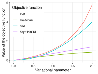
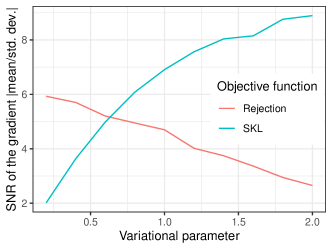
Figure 5: Left: objective functions for path optimization in a controlled experiment as a function of a variational parameter $\phi$. Right: signal-to-noise of corresponding gradient estimators on the same range of parameters.

Two objective functions were discussed in Section 3: one based on rejection rate statistics, i.e. Equation (14), and the symmetric KL divergence (SKL). In this section we perform controlled experiments comparing the signal-to-noise ratio of Monte Carlo estimators of the gradient of these two objectives. Let $G$ denote a Monte Carlo estimator of a partial derivative with respect to one of the parameters $\phi_{i}$. Refer to D for details on the stochastic gradient estimators. In this experiment we use i.i.d. samples so that the Monte Carlo estimators are unbiased, justifying the use of the variance as a notion of noise. Hence following Rainforth et al. (2018), we define the signal-to-noise ratio by $\text{SNR}=|{\mathbb{E}}[G]/\sigma[G]|$, where $\sigma[G]$ denotes the standard deviation of $G$. We use two chains with one set to a standard Gaussian, the other to a Gaussian with mean $\phi$ and unit variance. We show the value of the two objective functions in Figure 5 (left). The label “Rejection” refers to the expected rejection of the swap proposal between the two chains, $r$. We also show the square root of half of the SKL (“SqrtHalfSKL”), to quantify the tightness of the bound in Equation (17), while “Ineff” shows the rejection odds, $r/(1-r)$, called inefficiency in Syed et al. (2019).

Signal-to-noise ratio estimates were computed for each parameter $\phi_{i}\in\{0,1/5,2/5,\dots,2\}$. Each gradient estimate uses 50 samples, and to approximate the signal-to-noise ratio, the estimation was repeated 1000 times for each $\phi_{i}$ and objective function. The results are shown in Figure 5 (right), and demonstrate that in the regime of small rejection ($\lessapprox 30\%$), the gradient estimator based on the rejection objective has a superior signal-to-noise ratio compared to its SKL counterpart. However as $\phi$ increases and the two distributions become farther apart, the situation is reversed, providing empirical support for the surrogate objective for challenging path optimization problems.

Appendix G Experimental details

All the experiments were conducted comparing reversible PT, non-reversible PT and non-reversible PT based on the spline family with $K\in\{2,3,4,5,10\}$.

Every method was initialized at the linear path with equally spaced schedule, i.e. $\pi_{t}\propto\pi_{0}^{1-t/N}\pi_{1}^{t/N}$ with $N$ the number of parallel chains. All methods performed one local exploration step before a communication step.

To ensure a fair comparison of the different algorithms, we fixed the computational budget to a pre-determined number of samples in each experiment. Reversible PT used the budget to perform local exploration steps followed by communication steps. In non-reversible PT the computational budget was used to tune the schedule according to the procedure described in Syed et al. (2019, Section 5.1). For non-reversible PT with path optimization, the computational budget was divided equally over a fixed number of scans of Algorithm 2, where a scan corresponds to one iteration of the for loop.

Optimization of the spline annealing path family was performed using the SKL surrogate objective of Equation 17. Adagrad was used for the optimization. The gradient was scaled elementwise by its absolute value plus the value of the knot component. Such scaling was necessary to limit the gradient in the interval $[-1,1]$, stabilizing the optimization and avoiding possible exploding gradients due to the transformation to log space.

To mitigate variance in the results due to randomness, we performed 10 runs of each method and averaged the results across the runs.

G.1 Gaussian

This experiment optimized the path between the reference $\pi_{0}=N(-1,0.01^{2})$ and the target $\pi_{1}=N(1,0.01^{2})$. We used $N=50$ parallel chains initialized at a state sampled from a standard Gaussian distribution. In this setting, $\pi_{t}$ has a closed form that can be shown to be $N\left(\frac{\eta_{1}(t)-\eta_{0}(t)}{\eta_{0}(t)+\eta_{1}(t)},\left(\frac{0.01^{2}}{\eta_{0}(t)+\eta_{1}(t)}\right)^{2}\right)$, therefore, in the local exploration step of parallel tempering we sampled i.i.d.  from $\pi_{t}$. The computational budget was fixed at 45000 samples. Non-reversible PT with optimized path divided the budget in 150 scans. Therefore, for every gradient step in Algorithm 2, the gradient was estimated with 300 samples. We used 0.2 as learning rate for Adagrad.

G.2 Beta-binomial model

The second experiment was performed on a conjugate Bayesian model. The model prior was $\pi_{0}(p)=\mathrm{Beta}(180,840)$. The likelihood was $L(x|p)=\mathrm{Binomial}(x|n,p)$. We simulated $x_{1},\ldots,x_{2000}\sim\mathrm{Binomial}(100,0.7)$, resulting in a posterior distribution $\pi_{1}(p)=\mathrm{Beta}(140180,60840)$. The prior is concentrated at 0.176 with a standard deviation of 0.0119. The posterior distribution is concentrated at 0.697 with a standard deviation of 0.001. We used $N=50$ parallel chains initialized at 0.5. Also in this experiment it is possible to compute $\pi_{t}$ in closed form. Let $S=\sum_{i=1}^{2000}x_{i}$, $R=2000\times 100$ then $\pi_{t}(p)=\mathrm{Beta}(179\eta_{0}(t)+(180+S-1)\eta_{1}(t)+1,839\eta_{0}(t)+(840+N-S-1)\eta_{1}(t)+1)$. Hence, in the local exploration step of parallel tempering we sampled i.i.d. from $\pi_{t}$. The computational budget was fixed at 45000 samples. Non-reversible PT with optimized path divided the budget in 150 scans. Therefore, for every gradient step in Algorithm 2, the gradient was estimated with 300 samples. We used 0.2 as learning rate for Adagrad.

G.3 Galaxy data

The third experiment was a Bayesian Gaussian mixture model applied to the galaxy dataset of Roeder (1990). We used six mixture components with mixture proportions $w_{0},\ldots,w_{5}$, mixture component densities $N(\mu_{i},1)$ for mean parameters $\mu_{0},\ldots,\mu_{5}$, and a binary cluster label for each data point. We placed a $\mathrm{Dir}(\boldsymbol{1})$ prior on the proportions, where $\boldsymbol{1}=(1,1,1,1,1,1)$ and a $N(150,1)$ prior on each of the mean parameters. We did not marginalize the cluster indicators, creating a multi-modal posterior inference problem over 94 latent variables. In this experiment we used $N=35$ chains. Mixture proportions were initialized at $1/6$, mean parameters were initialized at 0 and cluster labels were initialized at 0. The local exploration step involved standard Gibbs steps for the means, indicators, and proportions. To improve local mixing, we also included an additional Metropolis-Hastings step for the proportions that approximates a Gibbs step when the indicators are marginalized. We fixed the computational budget to 50000 samples, divided into 500 scans using 100 samples each. We optimized the path using Adagrad with a learning rate of 0.3.

G.4 Mixture model

The fourth experiment was a Bayesian Gaussian mixture model with mixture proportions $w_{0},w_{1}$, mixture component densities $N(\mu_{i},10^{2})$ for mean parameters $\mu_{0},\mu_{1}$, and a binary cluster label for each data point. We placed a $\mathrm{Dir}(1,1)$ prior on the proportions, and a $N(150,1)$ prior on each of the two mean parameters. We simulated $n=1000$ data points from the mixture $0.3N(100,10^{2})+0.7N(200,10^{2})$. We did not marginalize the cluster indicators, creating a multi-modal posterior over 1004 latent variables. We used $N=35$ chains. Mixture proportions were initialized at 0.5, mean parameters were initialized at 0 and cluster labels were initialized at 0. The local exploration step involved standard Gibbs steps for the means, indicator variables, and proportions. To improve local mixing, we also included an additional Metropolis-Hastings step for the proportions that approximates a Gibbs step when the indicators are marginalized. The computational budget was fixed at 25000 samples. Non-reversible PT with optimized path divided the budget in 50 scans. Therefore, for every gradient step in Algorithm 2, the gradient was estimated with 500 samples. We used 0.3 as learning rate for Adagrad. Results are shown in Figure 6.

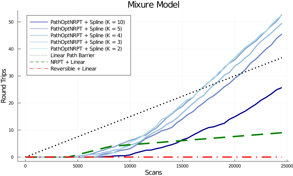
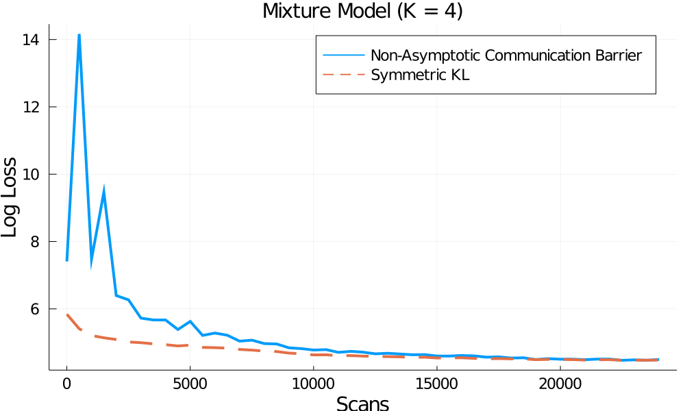
Figure 6: Top: Cumulative round trips averaged over 10 runs for the spline path with $K=2,3,4,5,10$ (solid blue), NRPT using a linear path (dashed green), and reversible PT with linear path (dash/dot red). The slope of the lines represent the round trip rate. Bottom: Non-asymptotic communication barrier from Equation 15 (solid blue) and Symmetric KL (dash orange) as a function of iteration for one run of PathOptNRPT + Spline ($K=4$ knots).

References

• Andrieu & Moulines (2006) Andrieu, C. and Moulines, E. On the ergodicity properties of some adaptive MCMC algorithms. Annals of Applied Probability, 16(3):1462–1505, 2006.
• Atchadé et al. (2011) Atchadé, Y. F., Roberts, G. O., and Rosenthal, J. S. Towards optimal scaling of Metropolis-coupled Markov chain Monte Carlo. Statistics and Computing, 21(4):555–568, 2011.
• Ballnus et al. (2017) Ballnus, B., Hug, S., Hatz, K., Görlitz, L., Hasenauer, J., and Theis, F. J. Comprehensive benchmarking of Markov chain Monte Carlo methods for dynamical systems. BMC Systems Biology, 11(1):63, 2017.
• Brekelmans et al. (2020) Brekelmans, R., Masrani, V., Bui, T., Wood, F., Galstyan, A., Steeg, G. V., and Nielsen, F. Annealed importance sampling with q-paths. arXiv:2012.07823, 2020.
• Costa et al. (2015) Costa, S. I., Santos, S. A., and Strapasson, J. E. Fisher information distance: A geometrical reading. Discrete Applied Mathematics, 197:59–69, 2015.
• Dabak & Johnson (2002) Dabak, A. G. and Johnson, D. H. Relations between Kullback-Leibler distance and Fisher information. Journal of The Iranian Statistical Society, 5:25–37, 2002.
• Desjardins et al. (2014) Desjardins, G., Luo, H., Courville, A., and Bengio, Y. Deep tempering. arXiv:1410.0123, 2014.
• Duchi et al. (2011) Duchi, J., Hazan, E., and Singer, Y. Adaptive subgradient methods for online learning and stochastic optimization. Journal of machine learning research, 12(7), 2011.
• Gelman & Meng (1998) Gelman, A. and Meng, X.-L. Simulating normalizing constants: From importance sampling to bridge sampling to path sampling. Statistical science, pp.  163–185, 1998.
• Geyer (1991) Geyer, C. J. Markov chain Monte Carlo maximum likelihood. Interface Proceedings, 1991.
• Grosse et al. (2013) Grosse, R. B., Maddison, C. J., and Salakhutdinov, R. R. Annealing between distributions by averaging moments. In Advances in Neural Information Processing Systems, 2013.
• Kamberaj (2020) Kamberaj, H. Molecular Dynamics Simulations in Statistical Physics: Theory and Applications. Springer, 2020.
• Katzgraber et al. (2006) Katzgraber, H. G., Trebst, S., Huse, D. A., and Troyer, M. Feedback-optimized parallel tempering Monte Carlo. Journal of Statistical Mechanics: Theory and Experiment, 2006(03):P03018, 2006.
• Lingenheil et al. (2009) Lingenheil, M., Denschlag, R., Mathias, G., and Tavan, P. Efficiency of exchange schemes in replica exchange. Chemical Physics Letters, 478(1-3):80–84, 2009.
• Müller & Bouckaert (2020) Müller, N. F. and Bouckaert, R. R. Adaptive parallel tempering for BEAST 2. bioRxiv, 2020. doi: 10.1101/603514.
• Okabe et al. (2001) Okabe, T., Kawata, M., Okamoto, Y., and Mikami, M. Replica-exchange Monte Carlo method for the isobaric–isothermal ensemble. Chemical Physics Letters, 335(5-6):435–439, 2001.
• Predescu et al. (2004) Predescu, C., Predescu, M., and Ciobanu, C. V. The incomplete beta function law for parallel tempering sampling of classical canonical systems. The Journal of Chemical Physics, 120(9):4119–4128, 2004.
• Rainforth et al. (2018) Rainforth, T., Kosiorek, A. R., Le, T. A., Maddison, C. J., Igl, M., Wood, F., and Teh, Y. W. Tighter variational bounds are not necessarily better. In International Conference on Machine Learning, 2018.
• Rischard et al. (2018) Rischard, M., Jacob, P. E., and Pillai, N. Unbiased estimation of log normalizing constants with applications to Bayesian cross-validation. arXiv:1810.01382, 2018.
• Roeder (1990) Roeder, K. Density estimation with confidence sets exemplified by superclusters and voids in the galaxies. Journal of the American Statistical Association, 85(411):617–624, 1990.
• Sakai & Hukushima (2016) Sakai, Y. and Hukushima, K. Irreversible simulated tempering. Journal of the Physical Society of Japan, 85(10):104002, 2016.
• Syed et al. (2019) Syed, S., Bouchard-Côté, A., Deligiannidis, G., and Doucet, A. Non-reversible parallel tempering: an embarassingly parallel MCMC scheme. arXiv:1905.02939, 2019.
• Tawn et al. (2020) Tawn, N. G., Roberts, G. O., and Rosenthal, J. S. Weight-preserving simulated tempering. Statistics and Computing, 30(1):27–41, 2020.
• Whitfield et al. (2002) Whitfield, T., Bu, L., and Straub, J. Generalized parallel sampling. Physica A: Statistical Mechanics and its Applications, 305(1-2):157–171, 2002.
• Woodard et al. (2009) Woodard, D. B., Schmidler, S. C., Huber, M., et al. Conditions for rapid mixing of parallel and simulated tempering on multimodal distributions. The Annals of Applied Probability, 19(2):617–640, 2009.
• Zhou et al. (2016) Zhou, Y., Johansen, A. M., and Aston, J. A. Toward automatic model comparison: An adaptive sequential Monte Carlo approach. Journal of Computational and Graphical Statistics, 25(3):701–726, 2016.