MnLargeSymbols’164 MnLargeSymbols’171
Imperial-TP-AT-2021-01
expansion of circular Wilson loopin superconformal quiver
M. Beccaria and A.A. Tseytlin111 Also at the Institute of Theoretical and Mathematical Physics, MSU and Lebedev Institute, Moscow.
a Università del Salento, Dipartimento di Matematica e Fisica Ennio De Giorgi,
and I.N.F.N. - sezione di Lecce, Via Arnesano, I-73100 Lecce, Italy b Blackett Laboratory, Imperial College London SW7 2AZ, U.K.
E-mail: matteo.beccaria@le.infn.it, tseytlin@imperial.ac.uk
Localization approach to superconformal quiver theory leads to a non-Gaussian two-matrix model representation for the expectation value of BPS circular Wilson loop . We study the subleading term in the large expansion of at weak and strong coupling. We concentrate on the case of the symmetric quiver with equal gauge couplings which is equivalent to the orbifold of the SYM theory. This orbifold gauge theory should be dual to type IIB superstring in . We present a string theory argument suggesting that the term in in the orbifold theory should have the same strong-coupling asymptotics as in the SYM case. We support this prediction on the gauge theory side by a numerical study of the localization matrix model. We also find a relation between the term in the Wilson loop expectation value and the derivative of the free energy of the orbifold gauge theory on 4-sphere.
1 Introduction and summary
Supersymmetric Wilson loop operators provide an important class of observables that shed light on the intricate structure of weak-strong coupling interpolation in the context of AdS/CFT duality. In special cases with extended supersymmetry the localization method [1] allows one to represent the expectation value of a supersymmetric loop in terms of a matrix model integral.
Here we will consider a particular supersymmetric gauge theory which is the quiver with two bi-fundamental hypermultiplets [2, 3, 4, 5]. In the “symmetric” case when the two ’t Hooft couplings , are equal this theory is equivalent to the orbifold of the SYM theory [6]. The orbifold theory has the same planar diagrams as the parent SYM theory [7], i.e. the two are closely related at large . The dual string theory should be the corresponding orbifold of the superstring, i.e. type IIB string on [8, 9].111 acts by flipping 4 of the 6 embedding coordinates of the 5-sphere, reflecting the 2+4 split of the SYM scalars between the vector multiplets and the hypermultiplets of the theory.
For each of the two factors of the quiver theory one may define -BPS circular Wilson loops coupled to the corresponding gauge and scalar fields ()
| (1.1) |
where we choose not to include the factor in front of the trace. For the orbifold theory their (normalized) expectation values are equal
| (1.2) |
and at large coincide [4] with the famous SYM result [10, 11, 12]
| (1.3) |
For general the expression for is given by a special non-Gaussian matrix model integral following from the localization approach [12]. In contrast to the SYM case where the corresponding matrix model is Gaussian leading to the closed expression [11, 12]
| (1.4) |
working out the expansion of turns out to be a non-trivial problem. Below we will address the question about the structure of the -dependent coefficients in the expansion of by considering separately the small and large limits.
On the dual string theory side, the expansion is the genus expansion, and the dependence of the coefficient in the analog of (1.4) corresponds to the string tension dependence of the partition function with world surface of topology of a disc with handles.
As discussed recently in [13], the strong coupling expansions of the -BPS circular Wilson loops in SYM and ABJM gauge theories with string duals defined on and have a remarkably similar structure. The string counterpart of the dominant at large () term in (1),(1.4) is the open-string partition function on the disk which contains an overall factor of the inverse closed string coupling
| (1.5) |
In the SYM case
| (1.6) |
In general, the presence of the universal prefactor in (1.5) follows from the structure of the 1-loop fluctuation determinants [14] appearing in the string partition function expanded near the AdS2 minimal surface (corresponding to the circular Wilson loop). In the case of genus surface the UV divergent part of the one-loop effective action reads [13]
| (1.7) |
where is 2d cutoff, is the AdS radius () and the coefficient turns out to be equal to the Euler number of the surface. The 2d UV divergence should be canceled by a universal superstring measure contribution involving only the string scale and not the AdS radius. Then the finite part of depends on through the term and thus the string partition function on a genus surface is proportional to , i.e.
| (1.8) |
Written in terms of and in (1.6) this matches the structure of the expansion of the exact SYM result in (1.4). One can also use similar considerations to predict the structure of the string theory expansions for other related observables [15].
It is important to emphasize the universality of the structure of the expansion in (1.8): it relies only on the fact that one expands near the AdS2 minimal surface embedded into the AdS3 part of AdSn space and should thus be valid also for the corresponding partition functions in the and superstring theories [13]. It should also apply to the orbifold theory: orbifolding the should not change the above argument determining the tension dependence from the way how the AdS radius appears in (1.7).222In the case of quiver theory which is the orbifold of the SYM and should be dual to the superstring on one has for the AdS radius and thus instead of (1.6) we get .
We thus conjecture that the same form of the large , strong coupling expansion (1.8) or (1.4) should also apply appear in the orbifold theory case, i.e.
| (1.9) |
where the coefficients will be different from the ones in (1.4).
In order to check the prediction (1.8),(1.9) for the large , strong-coupling expansion of we shall consider the genus one term corresponding to the leading correction to the planar part in (1). Normalizing to in (1) we have in both SYM and orbifold cases
| (1.10) |
where the form of the function will be our main focus in what follows. In the SYM case the expression for follows from the expansion of the exact Laguerre polynomial expression in (1.4) ( are modified Bessel functions of the first kind)
| (1.11) |
As discussed above, the leading strong-coupling behaviour of the genus one correction in
| (1.12) |
is consistent with the universal form of the string theory expansion in (1.4). Then according to (3.15) the same should be true also in the orbifold theory case, i.e.
| (1.13) |
where the value of the coefficient may of course be different from in the SYM case in (1.11). Confirming the prediction (1.13) starting from the localization matrix model representation for will be one of the aims of the present paper.
Summary of the results
As we shall see below, the matrix model representations for the orbifold gauge theory partition function on and for imply a remarkable relation between
| (1.14) |
and the limit of the deviation of the orbifold free energy from its SYM counterpart
| (1.15) | ||||
| (1.16) |
The leading term in cancels due to the planar equivalence between the orbifold theory and the two decoupled copies of the SYM theory.333More precisely, for the Wilson loops (1.2) the planar equivalence means that the normalized expectation value of an operator in one of the two factors of the quiver is the same as in the SYM theory. In general, the planar correlators of operators from symmetric (i.e. “untwisted”) sector should match between the orbifold and the parent SYM theory. For “extensive” quantities like the free energy (or conformal anomalies, correlators of total stress tensor, etc.) the results in the orbifold theory should match those of the two copies of the SYM. Using (1.15) the expected strong-coupling behaviour (1.13) of translates into the following scaling for the difference of free energies in (1.16) ()
| (1.17) |
In view of (1.16) this leads to a prediction about the strong coupling asymptotics of the leading correction to the planar part of the free energy of the orbifold theory.
Let us first recall that the free energy of SYM on should not be renormalized, i.e. should be given exactly by the familiar one-loop expression . Here is the conformal anomaly coefficient, , is the radius of , is a 4d UV cutoff and is a constant. Since the free energy is UV divergent, its finite part is not universal depending on a particular regularization scheme. The localization procedure [12] representing the free energy in terms of a finite matrix model integral with a simple -independent measure implicitly assumed a special regularization in which the renormalized SYM free energy is given by
| (1.18) |
as this expression follows simply from the Gaussian matrix model integral [16] (we drop an additive numerical constant).
From the dual string theory point of view, the gauge theory free energy is expected to be given by the string partition function or (at the tree level) by the IIB string effective action . Evaluated on (using (1.6) and ) the leading supergravity term here is where is the (logarithmically) IR divergent volume of unit-radius . Subtracting the IR divergence in using a particular AdS/CFT motivated prescription gives and thus one reproduces [16] the term in (1.18).444One way to understand the origin of the term is as follows. On AdS side the IR cutoff is measured in units of AdS radius . On the gauge theory side viewed as originating from the flat-space open string theory the natural UV cutoff is inverse of the string length . Thus the two cutoffs are related by the ratio .
The shift of in (1.18) should come from the 1-loop superstring correction (again proportional to ): this should follow the same pattern as found for the SYM conformal anomaly and Casimir energy in [17] (with only loops of short supergravity supermultiplets contributing). Other string tree level (e.g. , cf. [18]) and string loop corrections should vanish on maximally supersymmetric background.
Let us now turn to the orbifold theory that should be dual to the superstring on . Combining (1.16),(1.17) and (1.18) we get the following prediction
| (1.19) |
The leading term here is implied by the planar equivalence to the SYM and should follow again from the leading type IIB supergravity term evaluated on .555To recall, the orbifold projection of SYM giving the theory with two bi-fundamental hypermultiplets reduces the number of degrees of freedom and thus also the leading large term in the conformal anomaly coefficient from to which is twice the anomaly of a single copy of SYM theory at large . The exact expressions for the conformal anomaly coefficients of the quiver theory are and . On the supergravity side, replacing the coefficient in the above discussion by and noting that the volume of is half of the volume of we end up with as an overall coefficient. The planar equivalence also means that like in (1.18) this leading term should not get string tree level -corrections, i.e. they should still vanish when evaluated on .
One may attempt to give an independent string theory explanation of the subleading term in (1.19) without using the connection (1.15) to the Wilson loop. The string one-loop (genus one or order ) type IIB effective action is known to start with [19, 20, 21]. If we conjecture that when evaluated on the orbifold it is no longer zero then on dimensional grounds it should scale as , reproducing the subleading term in (1.19). If a non-zero contribution comes just due to the curvature singularity then it may not be proportional to the AdS5 volume so there will be no extra factor. The remaining puzzle is why the one-loop term may contribute to while the tree-level one should not, even though the two invariants have the same structure in type IIB string theory [22] (cf. the case of compactification of 6d orbifolds [23]).
Starting with the matrix model representation for we shall first study the structure of the function in (1.10) or in (1.14) at weak coupling. While the small expansion of in (1.11) has only rational coefficients, the coefficients in the expansion of in powers of are transcendental – proportional to the values of the Riemann -function
| (1.20) |
Thus may be formally used to parametrise the deviation of the orbifold theory result from the SYM one.
To find the strong-coupling expansion of requires a resummation of the weak coupling expansion. We shall study resummations of particular subclasses of terms proportional to monomials built out of . While this will not be enough to determine the correct strong coupling asymptotics of , this may still help to shed light on the general structure of this function.666A similar approach was applied [24] to superconformal theories admitting a large limit. Also, the use of sufficiently many terms in the perturbative series as a guide towards some non-perturbative features like singularities was emphasised in [25, 26].
Exploiting the relation (1.15) we shall compute up to order and also determine the resummation of all terms with the following types of coefficients involving particular and their powers
| (1.21) |
i.e. , etc. We find that they have the following behaviour at strong coupling
| (1.22) | ||||
| (1.23) |
The difference in these asymptotics implies that to find the correct strong coupling behaviour of the full one needs first to sum together different subsets of terms and only then expand the total at large .
Lacking an analytic method to compute at strong coupling we performed extensive numerical simulations of the orbifold matrix model to measure it. This required an extrapolation to large for finite , followed by an analysis of large region. We confirmed that the deviation from the SYM case starts only at the non-planar level. The numerical data agrees with the Padé-Borel resummation of the weak-coupling expansion up to moderate . At larger values of the coupling we found that the data is compatible with the following asymptotics
| (1.24) | ||||
| (1.25) |
The power of the leading asymptotics is thus consistent with the string theory prediction (1.13).777 If is set to be exactly , then the best fit value of the coefficient slightly changes to . It is interesting to notice that the values of the coefficients and are very close to the values of the corresponding coefficients in (1.11) in the SYM case up to a factor of and respectively. This suggests a conjecture that the exact form of the strong coupling expansion of is given by
| (1.26) |
It remains to be seen if one can prove this analytically.
One may wonder if the coefficient of the leading correction in may be found, as in the SYM case [27], also by considering the circular Wilson loop in -symmetric representation which should be described (for and =fixed) by a classical D3-brane solution. This does not seem possible as the D3-brane solution of [27] is restricted to AdS5 and thus the term in its action should have the same coefficient as in the SYM case, in contradiction with (1.25),(1.26). In fact, the D3-brane solution of [27] should be related not to the Wilson loop (1.2) of the orbifold theory but to the orbifold projection of the original circular Wilson loop in the SYM theory. The projection of the latter is represented by the correlator where in (1.1) correspond to the two factors of the orbifold theory. Starting with the Wilson loop in -symmetric representation one is to split it into the sum of products of the two representations. Then the D3-brane description may apply only to a special combination of the correlators where and are taken in the particular representations of the appearing in the product.888We thank N. Drukker for this suggestion. Assuming that -symmetric representation may be replaced by the -fundamental one (corresponding to multiply wrapped circle, cf. [28, 29]) one would expect to get the sum of the correlators
| (1.27) |
where is the Wilson loop in -fundamental representation. Rescaling the fields in (1.2) (or the corresponding matrices in the matrix model representation as in [11]) one would then end up with the sum of the correlators of the two fundamental Wilson loops in the quiver theory with the two ’t Hooft couplings . The resulting expression should simplify in the large limit and one expects it to be dominated by the “diagonal” term () with in the same representation. In section 6 we shall present numerical data indicating that the term in this correlator (with both Wilson loops taken in the fundamental representation of ) has a similar strong-coupling behaviour to found in the SYM case in (1.11).
Below we also computed numerically the individual Wilson loop (1.1) expectation values in the quiver with unequal couplings starting with the localization matrix model representation. Guided by the discussion in [4] here we considered the following analog of the ratio in (1.10)999 is found by interchanging and or .
| (1.28) |
where
| (1.29) |
The strong coupling result of [4] then implies that for any . We confirmed this prediction numerically by considering a particular value of the ratio of the two couplings (i.e. ) and measuring both Wilson loops and , thus effectively probing also the value . We found that the strong-coupling expansion of the function has the form where has a non-trivial dependence on . The numerical data for the function turns out to be compatible with the strong-coupling asymptotics in (1.24) with the exponent being again close to independently of , i.e. for both Wilson loops.
The rest of this paper is organized as follows. In section 2 we shall present the matrix model integral representation for the Wilson loop expectation value in the quiver theory which will be our starting point. In section 3 we shall consider the weak coupling expansion of the leading non-planar term the case of the orbifold theory organising it in terms of monomials of transcendental factors. We shall also derive the relation between the function and the free energy. In section 4 we shall perform a resummation of some subsets of terms and then expand them at strong coupling finding non-universal behaviour. In section 5 we shall consider the weak-coupling expansion in the case of non-symmetric quiver theory. Finally, in section 6 we shall present the results of the numerical computation of the matrix model integrals. Appendices A and B will contain some technical details of the computations in sections 3 and 4. In Appendix C we shall briefly discuss similar weak-coupling analysis of the Wilson loop in “orientifold” superconformal theory.
Note added in v4:
The coefficient in (1.17) was recently computed exactly in [30] with the result (also, coefficients of several subleading terms in (1.19) were also found). Since according to (1.15) the coefficient is related to the coefficient of term in or in (1.24) as this implies that (invalidating the conjecture in (1.26)). This value is substantially larger than the numerical estimate for in (1.25). This shows that the explored range of values was too narrow to reach the asymptotic regime where the leading term dominates. This is consistent with the presence of the subleading correction in in (1.17) (also established in [30]) that slows down the convergence.
2 Matrix model representation
Our starting point will be the localization matrix model representation for the partition function and the expectation values of the circular Wilson loops (1.1) in the superconformal quiver theory [12] (see also [2, 3, 4]). The partition function may be written as the integral over two sets of eigenvalues ()
| (2.1) |
where the -functions reflect the fact that we are considering the case (they may be ignored in strict planar limit) and101010 has the following representation in terms of the Barnes function The partition function is invariant under [3]. Note also that we ignored the instanton factor [12] in the integrand as we will be interested in perturbative expansion (see [3]).
| (2.2) |
Below we shall use to denote the (normalized) expectation value in the matrix model with the Gaussian measure so that (2.1) may be written as
| (2.3) | ||||
| (2.4) |
Here is the SYM partition function on .
The expectation values of the two Wilson loops (1.1) are given by
| (2.5) |
where is given by the same integral as in (2.1) and is normalized so that We use the notation for the diagonal matrix . The two expectation values (2.5) are equal (cf. (1.2)) at the orbifold point .
For large one may study the saddle points of the “effective action” in (2.1)
| (2.6) |
Differentiating over and introducing the densities
| (2.7) |
one finds the following saddle point equations [2, 3]
| (2.8) | ||||
| (2.9) | ||||
| (2.10) |
The large equivalence of the orbifold theory with the SYM follows [2, 4] from the fact that for the equations (2.8),(2.9) admit the symmetric Ansatz , and reduce to the saddle point equation for the Gaussian matrix model corresponding to the SYM case for which
| (2.11) |
The solution of the two integral equations (2.8),(2.9) in the large limit was studied in [2], showing that , and more recently in [4] where it was found that (see (1.29))
| (2.12) |
is the leading large , strong coupling term in the SYM result in (1).
3 Weak coupling expansion in the orbifold theory
Considering the orbifold theory case one can work out the weak-coupling expansion of by starting with the integral representation (2.1),(2.5) for finite . It may be formally written as a sum of functions multiplying particular products of values111111Similar expansions are found in other similar models, cf. [31, 32].
| (3.1) |
Here is given by (1.4) so that , etc., scale as at large . For small one has
| (3.2) |
To compute these functions starting with (2.1) let us note that using (2.2),(2.10) we get
| (3.3) | ||||
where we defined , (with ) and we also introduced the rescaled matrices (appearing in the exponent in (2.1))
| (3.4) |
3.1 Direct perturbative expansion
Separating different terms we may write in (3.3) as an expansion in
| (3.5) | ||||
| (3.6) |
Using (3.3) and computing (2.5) by first integrating out the dependence with the help of
| (3.7) |
we obtain for the coefficient functions in (3.1)
| (3.8) | ||||
| (3.9) |
where
| (3.10) |
This reduces the problem to evaluating correlators in one-matrix () Gaussian model.
Computing the Wilson loop correlator with normal ordered operators using that for the SYM case [11]
| (3.11) |
and applying the method described in Appendix A (see also [15]), we find ()
| (3.12) | |||
| (3.13) | |||
| (3.14) | |||
| (3.15) |
Since according to (3.11)
| (3.16) |
| (3.17) | ||||
| (3.18) |
The expressions (3.17) and (3.18) generate all terms proportional to and at leading and subleading order in in (3.1) within the weak coupling expansion. As expected, these functions scale as for large , i.e.
| (3.19) |
Similarly, the leading large terms in other coefficient functions in (3.1) are given by
| (3.20) | ||||
3.2 Leading non-planar correction and relation to free energy
Remarkably, the dependence on of the leading term in the functions in (3.1) follows the same pattern, i.e. is proportional to the Bessel function that appears in the leading order term in the SYM expression (3.16)
| (3.21) |
The power of is coming from the factors in (3.3) while the extra factor of (from the Bessel function factor ) has its origin in the Wilson loop operator insertion into the Gaussian matrix model integral at the leading order in large (cf. (2.5)). In particular, it comes from the term in ()
| (3.22) |
Separating this SYM Bessel function factor, the expression for the leading large term in in (3.1) can be written in terms of the function defined in (1.10),(1.14)
| (3.23) |
Here was given in (1.11) and the coefficients are found to be (cf. (3.1))
| (3.24) | ||||
In general, starting from the definition (2.5) of the Wilson loop expectation value (2.5) (e.g. for ), plugging in the expansion of in (3.5) and taking large we get, using that the integration over the “decoupled” variable gives an extra SYM factor (cf. (1.10),(1.14) and (2.3),(3.4),(3.11))
| (3.25) | ||||
| (3.26) |
We used (2.2),(3.3) to represent in (1.10),(1.14),(3.23) in terms of the Gaussian matrix model expectation value, traded the insertion of for the application of and used the symmetry of the integration measure. The expression (3.26) is equivalent to (1.15),(1.16) representing in terms of the free energy of the orbifold theory (see (2.3)).
As a check, using (3.3) one can compute the leading terms in the expansion of
| (3.27) |
Hence, for (3.26) we get
| (3.28) |
Thus the problem of computing in (3.23) is reduced to the calculation of the large limit of the free energy of the orbifold theory (which is finite for after the subtraction of the planar SYM term). This method is rather efficient as the direct computation of to higher orders without exploiting the resummation of the dependence in the factor would be prohibitively difficult. Using it we were able to push the calculation of the expansion of up to . In particular, the next five terms beyond (3.23) read
| (3.29) |
4 Resummation of particular transcendental contributions to
In an attempt to shed light on the structure of strong coupling limit of one may try to consider separate terms in the transcendental part of (3.1), resum their weak coupling expansion and then expand at strong coupling. As we shall see, this procedure will not give the correct strong-coupling limit of : the strong-coupling asymptotics of different functions will be different. That means that all such terms should first be summed up before taking the large limit.
As we shall show in Appendix B the terms in (3.1),(3.21) which are proportional to the single have the following coefficient functions
| (4.1) |
Summing all such terms in in (3.1), i.e. , we then get the corresponding contribution to or to in (1.14),(3.26)
| (4.2) |
We can resum this series by noting that
| (4.3) |
This gives ( are Bessel functions)
| (4.4) | ||||
| (4.5) |
Using the properties of the Mellin transform121212Defining the Mellin transform and considering the convolution we have Let be the fundamental strip of analyticity of . The asymptotic expansion of for is obtained by looking at the poles of in the region . Then the pole in the Mellin transform leads to the term in the original function. we find that the large asymptotics of (4.4) is
| (4.6) |
Similarly, we may consider all terms in (3.1) proportional to with (see Appendix B). We get the following analog of (4.2)
| (4.7) |
Summing this series as in (4.3),(4.4) we get
| (4.8) | ||||
| (4.9) |
Expanding at large here gives a different asymptotics than in (4.6)
| (4.10) |
As another example one may consider all the terms in involving only powers of . The resulting contribution takes a simple form (see Appendix B)
| (4.11) |
with the large asymptotics being again different from (4.6) and (4.10).
Using the general method described in Appendix B one is able to generalize (4.11) to the sum of all contributions involving arbitrary powers of and and also of
| (4.12) | |||
| (4.13) | |||
| (4.14) |
Comparing (4.11),(4.12) and (4.13) suggests that the strong coupling limit of the sum of monomials involving powers of the first constants should be (cf. (4.11),(4.12),(4.13))
| (4.15) |
Since the coefficient in (4.15) grows with , summing up such contributions after taking the large limit would not give a meaningful result.
5 Weak coupling expansion for non-symmetric quiver
Let us now discuss the expectation value of the Wilson loops (1.1),(2.5) in the case of the quiver for unequal couplings . We shall consider for definiteness . Setting
| (5.1) |
the generalization of (3.3) will read
| (5.2) |
It is then straightforward to compute the large expansion of the coefficient functions of the -monomial contributions to in the analog of (3.1). The first of them that generalizes (3.17) is
| (5.3) |
The planar (order ) contribution here agrees with the part of the SYM result in (1) expressed in terms of the effective coupling [33, 34, 31] ( there is )131313 In the case of the quiver the weak coupling expansion in the planar limit was analysed also in [35] and [25].
| (5.4) | ||||
| (5.5) |
Note that the subleading terms in (5) proportional to are similarly captured by the SYM term if we modify (5.5) as
| (5.6) |
One can also find the analog of in (3.1),(3.18) and the terms there can be generated from the SYM expression by the replacement generalizing (5.6)141414The limit of this expression is in agreement with Eq. (35) in [31].
| (5.7) |
This suggests that some essential features of the weak coupling expansion of the Wilson loop in the non-symmetric quiver case are already captured by the orbifold case () discussed above.
6 Numerical analysis of the quiver matrix model
One may try to compute the Wilson loop (1.1) numerically at finite and by starting with the matrix model representation (2.1),(2.5). While this is a finite dimensional integral, the fact that are interested in the limit makes the numerical integration hard. At the same time, we expect that, in the large limit, the relevant subset of the integration domain reduces to a neighbourhood of the saddle point solution. This problem is completely analogous to the one in the lattice field theory (where one computes quantum corrections by numerical path integration with ) and may thus be dealt with by the same Monte Carlo (MC) methods (see, for instance, [36]).
6.1 Orbifold theory
We analysed the Wilson loop expectation value (3.1) in the orbifold case by means of a Metropolis-Hastings Monte Carlo simulation [37] of the integral (2.1), a robust approach that does not require fine tuning.151515For other papers using MC methods in matrix models see, e.g., [38, 39, 40, 41, 42, 43] and section 6.5 of [44]. In the explored region of parameter space the Metropolis-Hastings algorithm turned out to be faster than the Hybrid Monte Carlo one, taking into account autocorrelation. The latter algorithm is expected to be preferable at higher and possibly more efficient for large-scale simulations which are beyond the scope of the present analysis.
Given a configuration of the eigenvalues corresponding to the two groups, the matrix integral (2.1) weights each observable , like the Wilson loop, with a positive number where corresponds to the total integrand in (2.1) including the Vandermonde factor. A Markov chain obeying detailed balance is built by making a local variation of and accepting the new configuration if or, in the case , with probability . We tuned the local changes of configuration in order to have an acceptance probability around 50-60% which is a reasonable choice. Iterating this procedure produces a sequence of configurations distributed according to and one can measure the quantum expectation value as the ensemble average . The sequence is correlated and its autocorrelation time has been measured at each data point and taken into account in the estimate of an error in this MC evaluation of . 161616As is well known (see, for instance, [45]), denoting by the average over MC realisations and assuming an exponential autocorrelation for the measurements , i.e. , the variance of the expectation value estimator is showing that the effective number of decorrelated measurements is roughly which is the factor entering the standard deviation of measurements .
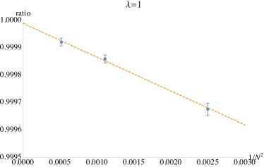
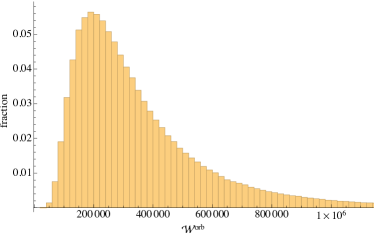
For each value of , we ran our code at various values of and fitted the Wilson loop measurements in order to extract the function (3.23) that governs the leading non-planar correction in (1.10). The procedure is illustrated in Fig. 1 (left) at the value . Fig. 1 (right) shows the histogram of measurements of the Wilson loop at , , as a sample point.
To provide non-trivial checks of the numerical code we considered the Wilson loop at which is a relatively weak coupling. From (3.23),(3.24) we see that for this value the leading contributions are negligible and we may assume that the same is true also for higher order contributions. Then
| (6.1) |
where the error is an estimate of the systematic error determined by including or not the the contribution of the terms explicitly computed above. The extrapolated slope from the finite MC simulations at shown in Fig. 1 (left) gives
| (6.2) |
which is thus consistent with the analytic estimate (6.1).
To compare results at higher values of we need to resum the perturbative expansion of in (3.23),(3.24),(3.29). We performed a Borel-Padé resummation for values of up to 50, see Fig. 2. The red line there is the perturbative series which is expected to converge for with partial sums blowing up beyond that value. 171717This is the radius of convergence of perturbative expansion in SYM theory in the planar limit. Its origin may be attributed to the form of the single-magnon dispersion relation, which follows from superconformal symmetry [46, 47] and it may also be found using the quantum algebraic curve approach [48]. That such a singularity is also present in the theories was first noticed in the mass-deformed theory case in [49]. The green line is the Padé approximant of the Borel improved series, while the blue line is the Borel transform, which is thus in good agreement with the numerical data points.
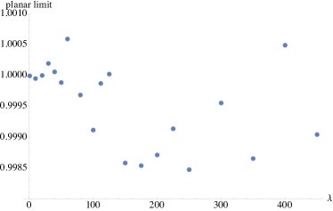
At higher values of we found similar extrapolations in . In Fig. 3 (left) we show the intercept of the extrapolation which is expected to be 1, see (3.1). This is a measure of the systematic error associated with the fit of the dependence. It increases with and we increased the maximal in order to keep it below the 0.2% level.181818Let us note that our numerical analysis is in a region of values of expected to be free from the instanton corrections which are weighted by the typical factors, at least up to instanton moduli space volume corrections [50].
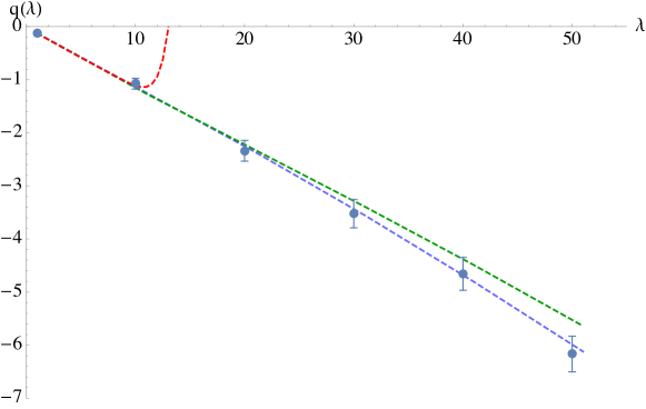
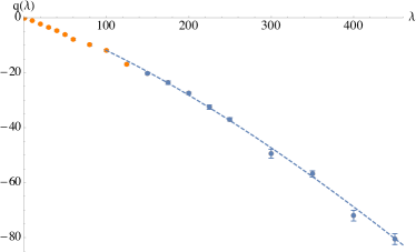
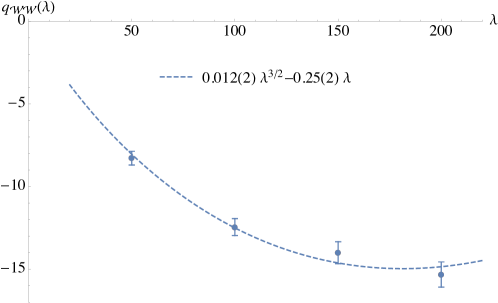
The resulting function computed for up to is shown in Fig. 3 (right). In the SYM theory, we know from (1.11) that at strong coupling which is valid with high accuracy already at . In the orbifold theory we find that is negative with a clear bending at large suggesting an asymptotic behaviour
| (6.3) |
The best fit of the blue data points in Fig. 3 (right) gives where the conservative error estimate includes statistics as well as the systematic effects due to the choice of fitting window. We estimated the latter by dropping some of the data points at smaller values of . This exponent is still to be taken with some caution since it is hard to say whether we are already in the asymptotic region but it appears to match the string theory prediction in (1.13) (see also (1.24),(1.25)).
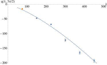
Finally, motivated by the discussion of the possible role of the D3-brane solution of [27] in the orbifold theory (see Introduction), we numerically computed the expectation value of the two Wilson loops (1.1) and determined (using the same fitting procedure as discussed above) the associated function defined as in (1.10)
| (6.4) |
The corresponding data points are shown in Fig. 6. They decrease to negative values with rate slower than the one observed in . A best fit of the form (1.24) with fixed at gives and . The coefficient has the opposite sign to the one in (1.25) and is close to the SYM value in (1.11). One possible interpretation of this result is that the “diagonal” correlator of the two Wilson loops in the fundamental representation exhibits the (at the leading non-planar order) the strong coupling behaviour which is expected from the D3-brane description, while other terms appearing in (1.27) are less important in the large limit.
6.2 Non-symmetric quiver
In the case of generic (non-zero) and the strong-coupling asymptotics of the Wilson loops is given by (2.12). We shall study the functions and in the ratio (1.28) of to the planar SYM result. We begin with the special point or (see (1.29))
| (6.5) |
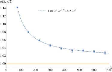
The numerical results are shown in Fig. 4. The left panel gives the function . As expected, it decreases for large towards 1 (this should hold for any , see (2.12)) and a good fit is
| (6.6) |
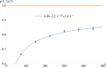
Measurement of the second Wilson loop provides the information about the same functions at the complementary value of the angle for which
| (6.7) |
The corresponding results are shown in Fig. 5. The best fit for the is191919The small but not negligible deviation of the estimated asymptotic value from 1 suggests that systematic errors should be reduced by extrapolations with larger values of . This could be related to the much large value of the correcting factor as compared to .
| (6.8) |
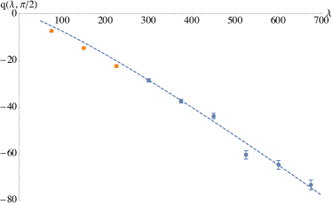
The function at and is shown in the right panels of Fig. 4 and Fig. 5. Our estimate for the exponent in the analog of (6.3) is and . Both values appear to be similar to the one found in the orbifold case (), i.e. . It would be desirable to push the MC simulation to larger values of the coupling , but that seems to require a dedicated analysis with a substantially increased computational power.
Acknowledgments
We would like to thank N. Drukker, S. Giombi, J. Russo, and K. Zarembo for useful discussions and comments on the draft. MB was supported by the INFN grant GSS (Gauge Theories, Strings and Supergravity). AAT was supported by the STFC grant ST/T000791/1.
Appendix A Multi-trace recursion relations and
The correlators in a Gaussian one-matrix model of the Wilson loop operator and a multi-trace chiral operator may be reduced to a differential operator over the coupling constant acting on (see (3.12)–(3.15)). This relation is exact at finite and is achieved by exploiting the fusion/fission relations [51] and the associated recursion relations on the expectation values
| (A.1) |
Let us consider as an example . We find ()
| (A.2) |
Doing Wick contractions leads to a combination of “single-trace” terms that can be traded for differential operators acting on and we finally obtain
| (A.3) |
This procedure can be easily coded in symbolic manipulation programs.
Appendix B Coefficient functions of -terms in
Here we shall provide some details of the weak-coupling computation of the coefficient functions in (3.1). Generalizing the calculation in (3.2), the contribution proportional to a single to the expectation value is given by
| (B.1) |
Using that the connected correlators are given by [24]
| (B.2) |
we get
| (B.3) |
To prove the relation (4.11) for the contribution to of the sum of terms proportional to powers of one may start with the following 2-matrix model with the term in the exponent representing the corresponding contribution coming from in (2.1),(3.3)202020In this special case there will be no difference between and cases.
| (B.4) |
Then according to (3.26),
| (B.5) |
Since the integrand in depends only on and , introducing the radial coordinates we get (ignoring irrelevant constant factor)
| (B.6) |
The large limit is found from a saddle point of the effective action Choosing the symmetric saddle with and integrating over the fluctuations gives
| (B.7) |
As a result, using (B.5) we find the strong-coupling asymptotics in (4.11). An alternative more rigorous and general approach is based on observing that in (B.4) may be represented as
| (B.8) |
As a result, we get again (B.7).
Similar approach can be used to derive (4.15) for the contribution of terms proportional to products of . For example, let us consider the terms. The new interaction term in the exponent in the analog of (B.4) will be
| (B.9) |
In this case instead of (B.8) we will need to consider
| (B.10) | ||||
| (B.11) |
Expanding (B.11), taking log and sending we find
| (B.12) |
Using this in (B) gives
| (B.13) |
As a result
| (B.14) |
which agrees with the results given in the main text.
Appendix C Wilson loop in “orientifold” superconformal theory
It is possible to give a similar discussion of the large expansion of the Wilson loop and the free energy in a particular superconformal gauge theory involving in addition to the vector multiplet also two hypermultiplets – in rank-2 symmetric and antisymmetric representations. This theory admits a regular ’t Hooft large limit and thus is similar to the quiver theory discussed above. It should be dual to the type IIB superstring on a particular orientifold AdS (see [52]).
This theory is one of the five cases of superconformal theories admitting a gauge group with generic [53]. The corresponding BPS circular Wilson loop is again equal to the SYM one at the planar level.212121This planar equivalence extends to classes of “even” observables, while “odd” sectors display deviations from SYM case already at the planar level [24]. Here we shall focus on the weak-coupling expansion of the first subleading correction, i.e. of the corresponding function defined as in (1.10).
From the supersymmetric localization, the free energy and the Wilson loop expectation value in this theory are described by the Hermitian one-matrix model of the similar structure as in (2.1) where instead of (3.3) now we have [54]
| (C.1) |
One can then organise the expansion of in powers of monomials of -constants as in (3.1). One finds that, as in the orbifold theory, at the leading non-planar level all appearing -monomials are multiplied by times a power of (cf. (3.21)). Explicitly, for defined as in (3.23), i.e. , we find
| (C.2) |
Like in (1.15),(1.16) there is again a relation between and the large limit of the difference of the orientifold and SYM free energies 222222Note that as both the orientifold theory and the SYM theory here are defined for a single copy of the coefficients in (C.3) are different from those in (1.15) by factors of 2.
| (C.3) |
References
- [1] V. Pestun et al., Localization techniques in quantum field theories, J. Phys. A50 (2017) 440301, [1608.02952].
- [2] S.-J. Rey and T. Suyama, Exact Results and Holography of Wilson Loops in N=2 Superconformal (Quiver) Gauge Theories, JHEP 01 (2011) 136, [1001.0016].
- [3] F. Passerini and K. Zarembo, Wilson Loops in N=2 Super-Yang-Mills from Matrix Model, JHEP 09 (2011) 102, [1106.5763]. [Erratum: JHEP10,065(2011)].
- [4] K. Zarembo, Quiver CFT at Strong Coupling, JHEP 06 (2020) 055, [2003.00993].
- [5] H. Ouyang, Wilson Loops in Circular Quiver SCFTs at Strong Coupling, JHEP 02 (2021) 178, [2011.03531].
- [6] A. E. Lawrence, N. Nekrasov and C. Vafa, On Conformal Field Theories in Four-Dimensions, Nucl. Phys. B 533 (1998) 199–209, [hep-th/9803015].
- [7] M. Bershadsky and A. Johansen, Large N limit of orbifold field theories, Nucl. Phys. B 536 (1998) 141–148, [hep-th/9803249].
- [8] S. Kachru and E. Silverstein, 4-D Conformal Theories and Strings on Orbifolds, Phys. Rev. Lett. 80 (1998) 4855–4858, [hep-th/9802183].
- [9] A. Gadde, E. Pomoni and L. Rastelli, The Veneziano Limit of Superconformal QCD: Towards the String Dual of ) Sym with = 2 , 0912.4918.
- [10] J. K. Erickson, G. W. Semenoff and K. Zarembo, Wilson loops in N=4 supersymmetric Yang-Mills theory, Nucl. Phys. B582 (2000) 155–175, [hep-th/0003055].
- [11] N. Drukker and D. J. Gross, An Exact prediction of N=4 SUSYM theory for string theory, J. Math. Phys. 42 (2001) 2896–2914, [hep-th/0010274].
- [12] V. Pestun, Localization of gauge theory on a four-sphere and supersymmetric Wilson loops, Commun. Math. Phys. 313 (2012) 71–129, [0712.2824].
- [13] S. Giombi and A. A. Tseytlin, Strong coupling expansion of circular Wilson loops and string theories in AdS and AdS, JHEP 10 (2020) 130, [2007.08512].
- [14] N. Drukker, D. J. Gross and A. A. Tseytlin, Green-Schwarz string in AdS(5) x S5: Semiclassical partition function, JHEP 04 (2000) 021, [hep-th/0001204].
- [15] M. Beccaria and A. A. Tseytlin, On the Structure of Non-Planar Strong Coupling Corrections to Correlators of BPS Wilson Loops and Chiral Primary Operators, JHEP 01 (2021) 149, [2011.02885].
- [16] J. G. Russo and K. Zarembo, Large Limit of Gauge Theories from Localization, JHEP 10 (2012) 082, [1207.3806].
- [17] M. Beccaria and A. A. Tseytlin, Higher spins in AdS5 at one loop: vacuum energy, boundary conformal anomalies and AdS/CFT, JHEP 1411 (2014) 114, [1410.3273].
- [18] S. S. Gubser, I. R. Klebanov and A. A. Tseytlin, Coupling constant dependence in the thermodynamics of N=4 supersymmetric Yang-Mills theory, Nucl. Phys. B534 (1998) 202–222, [hep-th/9805156].
- [19] M. B. Green, J. H. Schwarz and L. Brink, N=4 Yang-Mills and N=8 Supergravity as Limits of String Theories, Nucl. Phys. B198 (1982) 474–492.
- [20] D. J. Gross and E. Witten, Superstring Modifications of Einstein’s Equations, Nucl. Phys. B277 (1986) 1.
- [21] N. Sakai and Y. Tanii, One Loop Amplitudes and Effective Action in Superstring Theories, Nucl. Phys. B287 (1987) 457.
- [22] E. Kiritsis and B. Pioline, On threshold corrections in IIb string theory and (p, q) string instantons, Nucl. Phys. B 508 (1997) 509–534, [hep-th/9707018].
- [23] I. Antoniadis, R. Minasian and P. Vanhove, Noncompact Calabi-Yau manifolds and localized gravity, Nucl. Phys. B648 (2003) 69–93, [hep-th/0209030].
- [24] M. Beccaria, M. Billò, F. Galvagno, A. Hasan and A. Lerda, = 2 Conformal SYM theories at large , JHEP 09 (2020) 116, [2007.02840].
- [25] B. Fiol, J. Martfnez-Montoya and A. Rios Fukelman, The planar limit of = 2 superconformal quiver theories, JHEP 08 (2020) 161, [2006.06379].
- [26] B. Fiol, J. Martínez-Montoya and A. Rios Fukelman, The planar limit of superconformal field theories, JHEP 05 (2020) 136, [2003.02879].
- [27] N. Drukker and B. Fiol, All-genus calculation of Wilson loops using D-branes, JHEP 02 (2005) 010, [hep-th/0501109].
- [28] S. A. Hartnoll and S. Kumar, Higher Rank Wilson Loops from a Matrix Model, JHEP 08 (2006) 026, [hep-th/0605027].
- [29] S. Yamaguchi, Semi-Classical Open String Corrections and Symmetric Wilson Loops, JHEP 06 (2007) 073, [hep-th/0701052].
- [30] M. Beccaria, G. P. Korchemsky and A. A. Tseytlin, Strong coupling expansions in superconformal theories and the Bessel kernel, 2207.11475.
- [31] V. Mitev and E. Pomoni, Exact bremsstrahlung and effective couplings, JHEP 06 (2016) 078, [1511.02217].
- [32] F. Galvagno and M. Preti, Chiral correlators in = 2 superconformal quivers, JHEP 05 (2021) 201, [2012.15792].
- [33] E. Pomoni, Integrability in Superconformal Gauge Theories, Nucl. Phys. B 893 (2015) 21–53, [1310.5709].
- [34] V. Mitev and E. Pomoni, Exact effective couplings of four dimensional gauge theories with 2 supersymmetry, Phys. Rev. D 92 (2015) 125034, [1406.3629].
- [35] A. Pini, D. Rodriguez-Gomez and J. G. Russo, Large correlation functions 2 superconformal quivers, JHEP 08 (2017) 066, [1701.02315].
- [36] H. J. Rothe, Lattice Gauge Theories: an Introduction, vol. 43. 1992.
- [37] K. Binder and D. W. Heermann, Monte Carlo Simulation in Statistical Physics. An Introduction, 4th edition. Springer, 2002.
- [38] J. Ambjorn, K. Anagnostopoulos, W. Bietenholz, T. Hotta and J. Nishimura, Monte Carlo Studies of the Dimensionally Reduced 4-D Superyang-Mills Theory, in Workshop on Current Developments in High-Energy Physics: Hep 2000, 4, 2000. hep-th/0101084.
- [39] J. Ambjorn, K. Anagnostopoulos, W. Bietenholz, T. Hotta and J. Nishimura, Monte Carlo Studies of the IIB Matrix Model at Large N, JHEP 07 (2000) 011, [hep-th/0005147].
- [40] M. Hanada, M. Honda, Y. Honma, J. Nishimura, S. Shiba and Y. Yoshida, Numerical Studies of the Abjm Theory for Arbitrary at Arbitrary Coupling Constant, JHEP 05 (2012) 121, [1202.5300].
- [41] N. Sasakura and S. Takeuchi, Numerical and Analytical Analyses of a Matrix Model with Non-Pairwise Contracted Indices, Eur. Phys. J. C 80 (2020) 118, [1907.06137].
- [42] N. Sasakura, Numerical and Analytical Studies of a Matrix Model with Non-Pairwise Contracted Indices, PoS CORFU2019 (2020) 192, [2004.07419].
- [43] N. Tanwar, Monte Carlo Simulations of BFSS and IKKT Matrix Models, Master’s thesis, IISER Mohali, 6, 2020.
- [44] A. Joseph, Markov Chain Monte Carlo Methods in Quantum Field Theories: a Modern Primer, in 2019 Joburg School in Theoretical Physics: Aspects of Machine Learning, 12, 2019. 1912.10997.
- [45] A. Sokal, Monte carlo methods in statistical mechanics: foundations and new algorithms, in Functional integration, pp. 131–192. Springer, 1997.
- [46] N. Beisert, V. Dippel and M. Staudacher, A Novel Long Range Spin Chain and Planar Super Yang-Mills, JHEP 07 (2004) 075, [hep-th/0405001].
- [47] N. Beisert, B. Eden and M. Staudacher, Transcendentality and Crossing, J. Stat. Mech. 0701 (2007) P01021, [hep-th/0610251].
- [48] N. Gromov, Introduction to the Spectrum of SYM and the Quantum Spectral Curve, 1708.03648.
- [49] J. G. Russo and K. Zarembo, Evidence for Large-N Phase Transitions in * Theory, JHEP 04 (2013) 065, [1302.6968].
- [50] J. Russo and K. Zarembo, Massive Gauge Theories at Large N, JHEP 11 (2013) 130, [1309.1004].
- [51] M. Billo, F. Galvagno, P. Gregori and A. Lerda, Correlators between Wilson loop and chiral operators in conformal gauge theories, JHEP 03 (2018) 193, [1802.09813].
- [52] I. P. Ennes, C. Lozano, S. G. Naculich and H. J. Schnitzer, Elliptic Models, Type IIB Orientifolds and the AdS / CFT Correspondence, Nucl. Phys. B591 (2000) 195–226, [hep-th/0006140].
- [53] I. G. Koh and S. Rajpoot, Finite Extended Supersymmetric Field Theories, Phys. Lett. 135B (1984) 397–401.
- [54] M. Billò, F. Galvagno and A. Lerda, BPS wilson loops in generic conformal = 2 SU(N) SYM theories, JHEP 08 (2019) 108, [1906.07085].