Scalable nonparametric Bayesian learning for
heterogeneous and dynamic velocity fields

Abstract

Analysis of heterogeneous patterns in complex spatio-temporal data finds usage across various domains in applied science and engineering, including training autonomous vehicles to navigate in complex traffic scenarios. Motivated by applications arising in the transportation domain, in this paper we develop a model for learning heterogeneous and dynamic patterns of velocity field data. We draw from basic nonparameric Bayesian modeling elements such as hierarchical Dirichlet process and infinite hidden Markov model, while the smoothness of each homogeneous velocity field element is captured with a Gaussian process prior. Of particular focus is a scalable approximate inference method for the proposed model; this is achieved by employing sequential MAP estimates from the infinite HMM model and an efficient sequential GP posterior computation technique, which is shown to work effectively on simulated data sets. Finally, we demonstrate the effectiveness of our techniques to the NGSIM dataset of complex multi-vehicle interactions.

1 Introduction

A common theme arising in many modern engineering applications is that there often is a large amount of data available via spatiotemporal dynamics generated in a potentially fast-paced and highly heterogeneous environment; yet there is a need to extract meaningful and interpretable patterns out of such complexities in a computationally efficient way. The learned patterns further enhance the user’s understanding and improve subsequent decision-making. While there are many examples in a variety of domains, what motivates our present work the most is the analysis of traffic flow patterns out of high-volume and streaming measurements of vehicles passing through a busy thoroughfare.

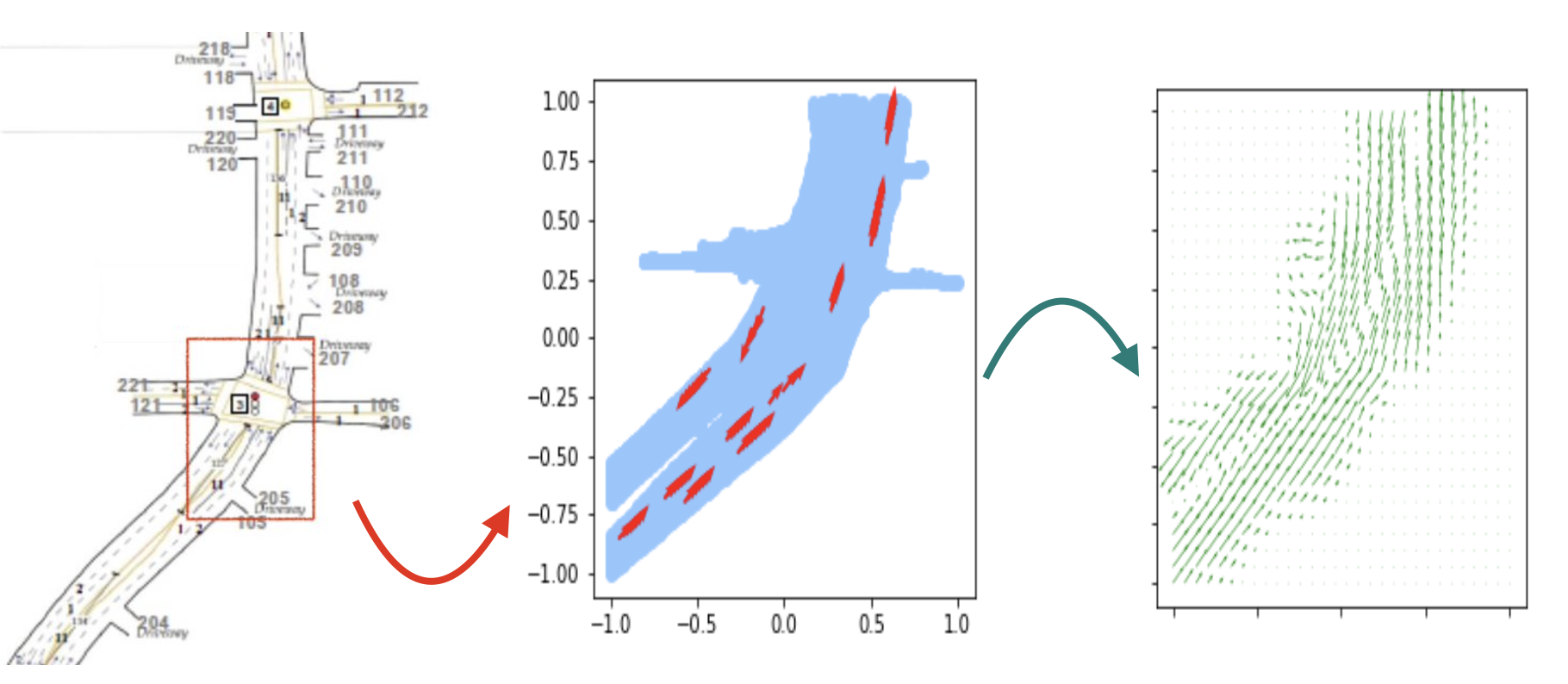
Figure 1: Left figure shows a portion of a Los Angeles boulevard, middle figure shows a frame of traffic presence passing through an intersection; right figure shows the corresponding traffic flow pattern represented as a velocity field on $\mathbb{R}^{2}$ obtained by our method.

A newcomer to a large and busy city may be initially shocked upon observing a bewildering range of individual driving behaviors and of cars moving in varying speeds and directions, competing and challenging for an open lane at any given moment. Yet, underneath this seemingly intractable complexity, one may eventually find the calming ebbs and flows of movements regulated by traffic control systems and the rhythm of the day. Such patterns of traffic flows can be represented by a two-dimensional velocity field indexed on a two-dimensional plane (see Fig. 1 for an illustration). The velocity field at a given time point records the expected velocity vector at different locations, if a car is present there at that moment. Unless there is an unusual disruption, one expects that the velocity vector varies smoothly, both in direction and magnitude, through the spatial domain. Thus, we adopt the viewpoint that a smooth vector field is a useful mathematical device to describe the current state of traffic flow at any given moment (Guo et al., 2019; Joseph et al., 2011; Chen et al., 2016).

In this paper, motivated by the aforementioned application, and to provide a fast posterior inference algorithm for parameters and quantities of interest, we aim to create a probabilistic (Bayesian) model for learning smooth vector field patterns out of heterogeneous and dynamic time series data. Our starting point is to model a smooth velocity field after a multi-response Gaussian process defined on a spatial domain, an idea that was also explored in  (Kim et al., 2011). To account for the temporal dynamics of spatial patterns, we employ a discrete-time hidden Markov chain that operates on the state space of smooth functions (representing the vector fields endowed by a Gaussian process prior). The vector fields are not observed directly; one only has access to frames of traffic passing through the road (see Fig. 1). Moreover, to account for the highly heterogeneous environment of movements, we allow the number of hidden states to be unbounded. This is achieved by drawing from the powerful nonparametric Bayesian elements of infinite hidden Markov models (HMM) and hierarchical Dirichlet processes (HDP) (Beal et al., 2002; Teh et al., 2006).

In short, we propose an infinite hidden Markov model, in which the underlying Markov chain operates on the space of Gaussian process vector fields, and the measurement noise model also follows that of a Gaussian distribution. Although the existing modeling elements are well-studied and have been explored in a wide range of applications, viz. Dirichlet processes for modeling heterogeneity (Ferguson, 1973; Antoniak, 1974; Ghosal & van der Vaart, 2017), hidden Markov models (Rabiner, 1989) and its infinite version (Beal et al., 2002; Teh et al., 2006) for time series analysis, and Gaussian processes for spatial data (Cressie, 1993; Kim et al., 2011), combining all such elements into a single nonparametric Bayesian modeling framework and applying it to high-dimensional velocity field data seems new and quite exciting for the application we have in our hand.

Due to the complexity of the proposed model, a particular focus of this work is on the development of a scalable approximate inference method to overcome the shortcoming of existing computational approaches. The standard techniques for Bayesian inference include MCMC (Gelfand & Smith, 1990; Fox et al., 2009) or variational inference (VI) (Blei et al., 2003; Foti et al., ). Due to the large number of latent variables in combination with complex modeling structures, MCMC algorithms tend to be inefficient. On the other hand, VI algorithms (cf. (Jordan et al., 1999; Blei & Jordan, 2006; Hoffman et al., 2013; Mandt et al., 2017)) are known to have difficulty producing statistically accurate posterior distributions, especially for finite samples. Our computational innovations include employing sequential MAP estimates from the infinite HMM model and efficient sequential GP posterior computation techniques. The latter techniques are crucial in overcoming very large covariance matrix, which is a consequence of the GP observed at a large number of spatial locations. They include using a block matrix inversion matrix using Schur’s complement. As we demonstrate in Table 1 and 3, these innovations allow us to analyze 10,000 total observations in around two minutes.

In summary, our contributions in this work are three-fold. Firstly, we study an infinite hidden Markov model on state space of multi-dimensional vector fields supported by a smooth Gaussian process prior. Secondly, we provide explicit computations via MAP estimates and devise a fast inference algorithm for the proposed model. Thirdly, the application to understanding of traffic encounters is a novel utilization of the model and the algorithm.

Other related work include (Fox et al., 2011), in which an infinite HMM combined with HDP has been used successfully to model speaker diarization behavior (Fox et al., 2011). By contrast, our work appeals to an infinite HMM for the high-dimensional velocity field hidden state space. There have also been prior work that combines both DP and GP modeling elements  (Guo et al., 2019; Joseph et al., 2011; Chen et al., 2016). The temporal modeling of the patterns in our work brings forward a novel aspect to the application perspective, which is potentially useful in improving autonomous vehicles based on interpretable learned patterns. Moreover, previous implementations of the DP-GP algorithms (Guo et al., 2019) are incapable of dealing with presence of large number of agents in each temporal epoch. As demonstrated in Section 5, our computational techniques help to overcome this shortcoming effectively.

The remainder of the paper is organized as follows. In section 2 we briefly review existing ideas necessary for the remainder of the paper, section 3 describes our model. Section 4 harps on the inference algorithm while section 5 demonstrates experimental results on simulated datasets and NGSIM traffic data.

2 Preliminaries

In this section, we briefly describe several key Bayesian nonparametric modeling elements for clustering data based on latent topics with unknown number of clusters and latent temporal dynamics. We also describe Gaussian processes and multivariate response Gaussian processes, which we use as the prior on the space to smooth velocity fields.

2.1 Infinite HMM

The infinite hidden Markov model was first proposed in (Beal et al., 2002) and subsequently shown to be an instance of the general Hierarchical Dirichlet process model of (Teh et al., 2006). We describe the infinite HMM setup as follows.

Assume that the behavioral outcome observed at each time-point is a noisy version of a specific underlying pattern among infinitely many such possible patterns. Let $\phi_{1},\phi_{2},\dots\overset{iid}{\sim}H$ be used to denote the underlying patterns, with $\phi_{k}$ used to assemble the pattern associated with the $k^{th}$ component. On the other hand, at each time point $t$, we have a random variable, $s_{t}\in\mathbb{N}$, which denotes which pattern is active at time $t$. The key assumption underlying the (hidden) Markov model structure is that the active pattern at time $t$ conditioned on the active pattern at $t-1$ is independent of prior history of active patterns.

Specific to the infinite HMM setup, the choice of pattern at each step $t$ affects the hidden pattern active at $t+1$ via an oracle value $o_{t}$. If $o_{t}=0$, the choice of active pattern depends on the historical counts of respective pattern types, whereas if $o_{t}=1$, an oracle is invoked. Before we mathematically define the model, we introduce some notations for count variables that will be useful:

$$N^{(t)}_{j} =\sum_{u=1}^{t}\mathbbm{1}(s_{u}=j),\;n^{(t)}_{ij}=\sum_{u=1}^{t-1}\mathbbm{1}(s_{u}=i,s_{u+1}=j),$$ (1)

$$m^{(t)}_{j} =\sum_{u=1}^{t-1}\mathbbm{1}(s_{u+1}=j,o_{u}=1).$$ (2)

They respectively represent the number of times a state has been visited, the number of transitions from one state to another, and the number of times a state has been visited while invoking the oracle until time $t$. If $s_{1},\dots,s_{t}$ are the states for time points up to $t$ and $\tilde{K}^{(t)}$ are the number of distinct states explored, the infinite HMM model (with parameters $\alpha$ and $\gamma$) is completely described by the process of sampling $s_{t+1}$. This is done in the following manner.

$$\mathbb{P}(s_{t+1}=j,o_{t}=0\mid s_{t}=i,n,\alpha) =\frac{n_{ij}^{(t)}}{\sum_{j^{\prime}=1}^{\tilde{K}^{(t)}}n_{ij^{\prime}}^{(t)}+\alpha}$$

$$\mathbb{P}(o_{t}=1\mid s_{t}=i,n,\alpha) =\frac{\alpha}{\sum_{j^{\prime}=1}^{\tilde{K}^{(t)}}n_{ij^{\prime}}^{(t)}+\alpha}$$ (3)

Moreover, given that we have defaulted to an oracle ($o_{t}=1$), the transition satisfies

$$s_{t+1}\mid s_{t}=i,m,\gamma,o_{t}=1\sim$$

$$\sum_{j=1}^{\tilde{K}^{(t)}}\frac{m_{j}^{(t)}}{\sum_{j^{\prime}}m_{j}^{(t)}+\gamma}\delta_{j}+\frac{\gamma}{\sum_{j^{\prime}}m_{j}^{(t)}+\gamma}\delta_{\tilde{K}^{(t)}+1}$$ (4)

When $K+1$ is chosen, the system explores a new state $K+1$ and gets $\phi_{K+1}$ previously unused. This two layer structure achieves the same objective as the HDP (described in the Appendix). Now to complete the HMM structure, when $s_{t}=k$, we assume that the observation emission follows $x_{t}\sim F(\cdot|\phi_{k})$. This completes the description of the Infinite HMM model. The model is illustrated in Figure 2.

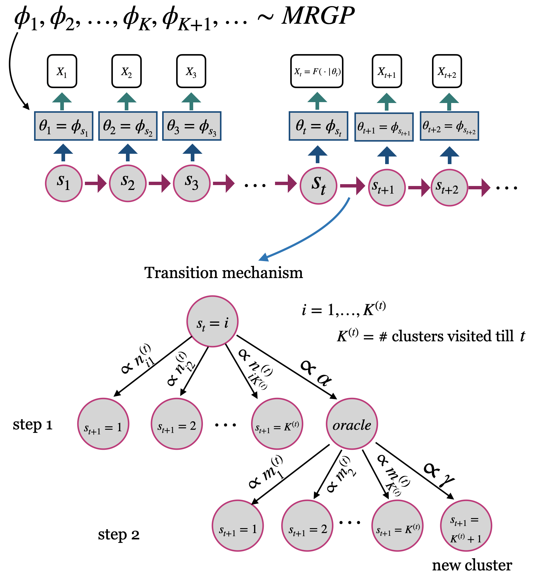
Figure 2: Graphical illustration of the infinite HMM model.

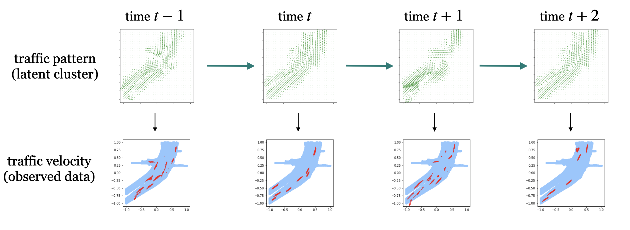
Figure 3: A simple example of our model: at each time $t$, a latent cluster is chosen and based on that traffic pattern, we observe some real data — velocity vectors at some spatial points. Note in this example the clusters at time $t$ and $t+2$ are same — the frames at these time points correspond to the same traffic pattern.

2.2 Gaussian process

Gaussian processes (GP) provide a mechanism to model (smooth) functions on arbitrary index spaces. A stochastic process $\{X(t):X(t)\in\mathbb{R},\ t\geq 0\}$ is called a GP with mean $m(\cdot)$ and covariance kernel $K(\ast,\ast)$ if for any finite $T:=\{t_{1},\dots,t_{k}\}\subset[0,\infty)$,

$$(X(t_{1}),\dots,X(t_{k}))\sim\mathcal{N}\left(m\big{|}_{T},K\big{|}_{T\times T}\right),$$ (5)

where $m\big{|}_{T}=(m(t_{1}),\dots,m(t_{k}))$ and $K\big{|}_{T\times T}(i,j)=K(t_{i},t_{j}),\text{ }1\leq i,j\leq k$.

2.3 Multi-response Gaussian process

Before we introduce the multi-response Gaussian process (MRGP), we need to define the matrix normal distribution. This distribution will allow us to assign probability to the stochastic process.

A random matrix $Z_{k\times d}$ is said to follow a matrix normal distribution with parameters $M_{k\times d},U_{k\times k}$ and $V_{d\times d}$, i.e., $Z\sim\mathcal{MN}_{k\times d}(M,U,V)$, if

$$\text{vec}(Z)\sim{\mathcal{N}}_{kd}(\mathrm{vec}(M),V\otimes U).$$ (6)

The Kronecker product is denoted by $\otimes$ and ${\mathrm{vec}(M)}$ signifies the vectorization of $M$. We now define the MRGP.

Let $f:\mathbb{R}^{p}\to\mathbb{R}^{d}$ and we write for $z\in\mathbb{R}^{p}$, $f(z)=(f_{1}(z),\dots,f_{d}(z))^{T}\in\mathbb{R}^{d}$. Given a kernel $K:\mathbb{R}^{p}\times\mathbb{R}^{p}\to\mathbb{R}^{+}$ and a mean function $\mu:\mathbb{R}^{p}\to\mathbb{R}^{d}$, we write $f\sim MRGP(\mu,K,\rho)$ if for any finite $n$ and any $z_{1},\dots,z_{n}\in\mathbb{R}^{p}$, we posit the following matrix normal distribution

$$f(z_{1:n})=\begin{pmatrix}f_{1}(z_{1})&\dots&f_{d}(z_{1})\\ f_{1}(z_{2})&\dots&f_{d}(z_{2})\\ \vdots&\ddots&\vdots\\ f_{1}(z_{n})&\dots&f_{d}(z_{n})\end{pmatrix}\sim MN_{nd}\left(M,\Sigma,\Omega\right).$$ (7)

Here, $z_{1:n}=(z_{1},\dots,z_{n})$, $M\in\mathbb{R}^{n\times d}$ with $M_{ij}=\mu_{j}(z_{i})$,

$$\Sigma =\begin{pmatrix}K(z_{1},z_{1})&K(z_{1},z_{2})&\dots&K(z_{1},z_{n})\\ K(z_{2},z_{1})&K(z_{2},z_{2})&\dots&K(z_{2},z_{n})\\ \vdots&\vdots&\ddots&\vdots\\ K(z_{n},z_{1})&K(z_{n},z_{2})&\dots&K(z_{n},z_{n})\end{pmatrix}$$ (8)

$$\Omega =\begin{pmatrix}1&\rho&\dots&\rho\\ \rho&1&\dots&\rho\\ \vdots&\vdots&\ddots&\vdots\\ \rho&\rho&\dots&1\end{pmatrix}.$$ (9)

In other words, $\Sigma$ captures the covariance across the rows and $\Omega$ across the columns. In our case, we fix $\Omega$ as the equicorrelation($\rho$) matrix of size $d\times d$ and $\Sigma$ is a $n\times n$ matrix formed using the kernel $K$ as $\sigma_{ij}=K(z_{i},z_{j})$.

We choose $\mu\equiv 0$ and we use the Radial Basis Function (RBF) kernel $K(x_{1},x_{2})=\sigma_{0}^{2}\exp\left\{-\frac{\left\lVert x_{1}-x_{2}\right\rVert^{2}}{2\ell_{0}^{2}}\right\}$ where $\sigma_{0}^{2}$ is the kernel variance and $\ell_{0}$ is the kernel lengthscale.

3 Data model

We assume that the data is spatio-temporal in nature. More specifically, given an underlying spatial domain $\mathcal{B}\subset\mathbb{R}^{p}$. Let us denote $\mathcal{F}=\{f:B\to\mathbb{R}^{d}\}$ as a space of functions with domain in $B$ and range in $\mathbb{R}^{d}$. We are given a stochastic process, $\{X_{t}:X_{t}\in\mathcal{F},\ t\geq 0\}$, which we wish to model. In other words, at each discrete time-point $t=1,2,\dots,T$, we have a system that outputs a function. Moreover, at each time point $t$, we only observe the outputs $X_{t}(z_{1}),\ldots,X_{t}(z_{N})$, for some $z_{1},\ldots,z_{N}\in\mathcal{B}$.

The key assumption underlying our model is that there exist an unknown number of true patterns (or functions) $\phi^{0}_{1},\phi^{0}_{2},\dots\in\mathcal{F}$ which give rise to the observed patterns as follows. Suppose at time point $t$, pattern $s_{t}$ is active, then the observations at time point $t$ are modeled as:

$$X_{t}(z_{n}) \sim\mathcal{N}(\phi^{0}_{s_{t}}(z_{n}),\sigma^{2}\mathbbm{I})\qquad n=1,2,\ldots,N.$$ (10)

We next discuss how to model the random selection of patterns at each time $t$ by drawing from our intuition about modeling velocity flow patterns relevant to traffic movements. Traffic flow patterns at a time point are directly influenced by the patterns of traffic lights. How other patterns affect flow patterns might depend on the time of day, which in turn affect how the flow patterns behave locally in time. While it is expected that flow patterns at time points close to each other would be strongly dependent, it is reasonable to model the flow patterns as independent whenever they are separated by a large time interval. In that regard, Markov chains form the simplest objects to model changes in behavior locally across time. For this paper we will focus on 1-step Markov Chain via a hidden Markov model for choosing states. The movement of the Markov chain is guided by transition probabilities between different states. Since we want to be flexible about the number of states, we allow for an infinite number of latent states, each having an infinite length transition probability vector for moving to the next state. Infinite HMMs therefore provide an appropriate setup to model such transitions.

Moreover, we want to be flexible about the nature of the velocity flow. The basic assumption underlying a velocity flow is that each location in a region ($\mathcal{B}$ in this case) is associated with a velocity. The collection of all the velocities across all such locations is a velocity field. GPs are flexible objects for modeling arbitrary multivariate functions on spatial domains. We therefore assume that each hidden velocity field pattern, labelled as $\phi_{1},\phi_{2},\ldots$, (different from the true underlying patterns $\phi^{0}_{1},\phi^{0}_{2},\dots$ ) is modelled as realisations from a MRGP with RBF kernel $K(\cdot,\cdot)$ in a suitable domain.

Model:

The complete model is outlined as follows.

$$\phi_{1},\phi_{2},\dots&\sim MRGP(0,K,\rho)$$ (11)

$$s_{1},\dots,s_{T} \sim\text{infinite HMM}(\alpha,\gamma)$$

$$X_{t}(z_{n})\mid\{\phi_{k}\} \sim\mathcal{N}(\phi_{s_{t}}(z_{n}),\sigma^{2}\mathbbm{I}) t=1,2,\ldots,T;$$

$$n=1,2,\ldots,N.$$

Note that in the model, we assume that $z_{1},\ldots,z_{N}$ are common to all time-points $t$, but our model can be easily extended to the case of observing velocity flows in different locations across different time points. The analysis remains similar to the one performed below. We focus on this scenario to avoid over-burdening our notations.

The usefulness of the above model is multi-fold. First, it helps to extract each pattern of traffic movement corresponding to a given time point. Moreover, it provides us the ability to infer about the transition patterns. In the context of autonomous vehicles, while this is extremely useful to guide the vehicle about the current scenario of neighboring traffic, it also provides an understanding about what behavior to expect from neighboring vehicles at the next instant.

4 Fast sequential posterior computation for Gaussian process

The full posterior with the above model is a complex object. While MCMC updates can be extremely slow due to invoking of forward-backward algorithm (especially with high-dimensional calculations with GPs), approximate techniques such as variational inference can often lead to inaccurate estimates. We therefore focus on maximum a posteriori (MAP) estimates for inference.

Our particular inference scheme involves sequentially estimating the state variables, $s_{t}$, and oracle indicator variables, $o_{t}$ for $t=1,2,\ldots,T$ and the latent, spatial functions $\phi_{k}$ for $k=1,2,\ldots,\tilde{K}^{(t)}$. The steps for doing so via a one-pass MAP estimator are given in Algorithm 1. Before we elaborate on the computation of the different steps in Algorithm 1, the following notation will be helpful to describe this algorithm:

Let $\tilde{K}^{(t)}$ be the number of observed patterns until $t$. Also, let $\mathcal{H}_{t}=\biggr{\{}\phi_{1:\tilde{K}^{(t)}},o_{1:t},s_{1:t},\\ \hskip 40.00006pt\{m_{j}^{(t^{\prime})}\}_{k;t^{\prime}=1:t},\{n_{ij}^{(t^{\prime})}\}_{k,k^{\prime};t^{\prime}=1:t},\{N_{j}^{(t^{\prime})}\}_{j;t^{\prime}=1:t}\biggr{\}}$. Here, $m_{j}^{(t^{\prime})},n_{ij}^{(t^{\prime})},N_{j}^{(t^{\prime})}$ are as defined in Eq. (2).

4.1 Estimating state variable

Let $z^{t+1}_{1:n^{(t+1)}}$ denotes the locations of observation at time $t+1$. By Bayes’ rule, the posterior distribution of $s_{t+1}$ is

$$\operatorname{\mathbb{P}}(s_{t+1} =j\mid\mathcal{H}_{t},X_{1},X_{2},\ldots,X_{t+1})\propto$$ (12)

$$\operatorname{\mathbb{P}}(s_{t+1}=j|\mathcal{H}_{t})\operatorname{\mathbb{P}}(X_{t+1}(z^{t+1}_{1:n^{(t+1)}})\mid s_{t+1}=j,\mathcal{H}_{t})$$

for $j=1,2,\ldots,\tilde{K}^{(t)}+1$.

We can use the transition probabilities for infinite HMM given in Eq. (3) and Eq. (4) to get that

$$\operatorname{\mathbb{P}}(s_{t+1}=j\mid s_{t}=i,\mathcal{H}_{t})$$

$$= \begin{cases}\frac{n^{(t)}_{ij}}{\sum_{j^{\prime}=1}^{\tilde{K}^{(t)}}n^{(t)}_{ij^{\prime}}+\alpha}+\frac{\alpha m^{(t)}_{j}}{(\sum_{j^{\prime}=1}^{\tilde{K}^{(t)}}n^{(t)}_{ij^{\prime}}+\alpha)(\sum_{j^{\prime}=1}^{\tilde{K}^{(t)}}m^{(t)}_{j^{\prime}}+\gamma)},\\ \hskip 120.00018pt\text{ if }1\leq j\leq\tilde{K}^{(t)}\\ \frac{\alpha\gamma}{(\sum_{j^{\prime}=1}^{\tilde{K}^{(t)}}n^{(t)}_{ij^{\prime}}+\alpha)(\sum_{j^{\prime}=1}^{\tilde{K}^{(t)}}m^{(t)}_{j^{\prime}}+\gamma)},\text{ if }j=\tilde{K}^{(t)}+1.\end{cases}$$

The first line refers to some previous state $j$ being chosen at time $t+1$ and the first term is when it is chosen directly while the second term is for when it is chosen through the oracle. The second line refers to a new state being chosen $s_{t+1}=\tilde{K}^{(t)}+1$, which is only possible through the oracle. Eq. (4.1) defines a prior for $s_{t+1}$ given all the required terms.

The computation of the second term in the RHS of Eq. (12) is computed using Prop. 4.1 and is provided in the appendix.

4.2 Estimating oracle variable

The posterior distribution of $o_{t+1}$ is calculated using Bayes’ rule as follows.

For $j=1,2,\ldots,K^{(t)}+1$, $e\in\{0,1\}$, by Lemma A.1 in the appendix,

$$\operatorname{\mathbb{P}}(o_{t+1}=e \mid X_{t+1}(z^{t+1}_{1:n^{(t+1)}}),s_{t+1}=j,\mathcal{H}_{t})\propto$$ (14)

$$\operatorname{\mathbb{P}}(s_{t+1}=j\mid o_{t+1}=e,\mathcal{H}_{t})\operatorname{\mathbb{P}}(o_{t+1}=e\mid\mathcal{H}_{t}),$$

Recall that $o_{t}$ is a binary variable, which is 1 if $s_{t+1}$ was generated through the oracle and $0$ if $s_{t+1}$ was generated directly. We first describe the former case. For the first term in the RHS of Eq. (14), Eq. (4) tells us that

$$\operatorname{\mathbb{P}}(s_{t+1}=j\mid o_{t+1}=1,\mathcal{H}_{t})$$ (15)

$$= \begin{cases}m^{(t)}_{j}/(\sum_{j^{\prime}}m^{(t)}_{ij^{\prime}}+\gamma),\ j\in\{1,\dots,\tilde{K}^{(t)}\}\\ \gamma/(\sum_{j^{\prime}}m^{(t)}_{ij^{\prime}}+\gamma),\ j=\tilde{K}^{(t)}+1.\end{cases}$$

In other words, it is the probability that the oracle was invoked to generate the next hidden state, $j$. Using Eq. (3), we get that the second term in the RHS of Eq. (14) is

$$\operatorname{\mathbb{P}}(o_{t+1}=1\mid s_{t}=i,\mathcal{H}_{t})=\alpha/(\sum_{j}n^{(t)}_{ij}+\alpha).$$ (16)

This is the probability that the oracle is invoked at time $t+1$. While $s_{t}=i$ is contained in $\mathcal{H}_{t}$, we explicitly write it out to make clear that this probability depends on the number of transitions from state $i$.

We can then make similar calculations for $o_{t}=0$. For the first term, we have that

$$\operatorname{\mathbb{P}}(s_{t+1}=j\mid o_{t+1}=0,\mathcal{H}_{t})$$ (17)

$$= \begin{cases}n^{(t)}_{ij}/\sum_{j}n^{(t)}_{ij},\ \ j\in\{1,\dots,\tilde{K}^{(t)}\}\\ 0,\ \ \ \ \qquad j=\tilde{K}^{(t)}+1.\end{cases}$$

The second term is $1-\operatorname{\mathbb{P}}(o_{t+1}=1\mid s_{t}=i,\mathcal{H}_{t})$.

Input: Data $\{X_{t}\}_{t=1}^{\infty}$ fed sequentially. Hyperparameters $\sigma^{2}$,kernel $K$, locations $\{z^{t}_{1:n^{(t)}}\}_{t},\rho,\alpha,\gamma$.
Initialization:
For $t=1$, set $s_{t}=1,o_{t}=1,n^{(1)}=[0],m^{(1)}=[1]$
Update $\hat{\phi}_{1}$ using Proposition 4.1
Steps: For each time $t=1,2,\dots,T$

1. Set $\hat{s}_{t+1}\xleftarrow{}\operatorname*{arg\,max}_{j}\operatorname{\mathbb{P}}(s_{t+1}=j\mid\mathcal{H}_{t},x_{t+1})$ using (12), (4.1) and Proposition 4.1.

2. Set $\hat{o}_{t+1}\xleftarrow{}\operatorname*{arg\,max}_{e}\operatorname{\mathbb{P}}(o_{t+1}=e\mid x_{t+1},s_{t+1},\mathcal{H}_{t})$, using Eqs.(14), (15),(16) and (17).

3. Update $n^{(t)}_{\widehat{s}_{t},\widehat{s}_{t+1}},m^{(t)}_{\widehat{s}_{t+1}}$.

4. Update estimates for $\phi_{s_{t+1}}$ using the GP posterior discussed in (U.1) at the end of Section 4.3.

Output: $\widehat{s}_{t}$ and $\widehat{o}_{t}$ for $t=1,2,\ldots,T$ and $\hat{\phi_{k}}$ for $k=1,2,\ldots,K_{0}$

Algorithm 1 Sequential maximum a posteriori estimation for Infinite HMM-GP

These estimates, $\widehat{s}_{t+1}$ and $\widehat{o}_{t+1}$, are then used to update the $\phi_{\widehat{s}_{t+1}}$ and previous count variables. We describe how to efficiently sequentially update $\phi_{k}$ in the next section.

4.3 Estimating underlying patterns

We now discuss the estimation of underlying patterns $\phi_{1},\phi_{2},\ldots$ at time-step $t+1$.

Notations:

1. Let $T_{j}^{t}=\{t^{j}_{1},t^{j}_{2},\ldots,t^{j}_{j_{t}}\}$, $j_{t}\in\mathbbm{N}$, indicate all the times during for which $\widehat{s}_{t^{\prime}}=j$ for $t^{\prime}\leq t$.

2. Let $x_{t}=\text{vec}(X_{t}(z_{1:n^{(t)}}))$ be the $n^{(t)}d$ dimensional vector of observations at time $t$.

3. Moreover, let $\text{vec}\left((x^{t^{j}_{k}})\mid_{k=1:j_{t}}\right)$ be the $Nd$ ($N$ is the total number of locations among elements of $T_{j}^{t}$) dimensional vector obtained by stacking $x_{t^{j}_{k}}$, $k=1:j_{t}$, on top of one another.

4. Let $Z_{t}^{j}$ denote the collections of all the locations for observations across time-points in $T_{j}^{t}$. Then, let $K(Z_{t}^{j},Z_{t}^{j})$ denote the matrix $(K(z_{i},z_{j}))_{z_{i},z_{j}\in Z_{t}^{j}}$. Similarly, define $K(z,Z_{t}^{j})$,$K(Z_{t}^{j},z)$ and $K(z,z)$ for any $z\in\mathbb{R}^{p}$.

By the assumption of MRGP we have that,

$$\text{vec}\left((x^{t^{j}_{k}})\mid_{k=1:j_{t}}\right)\sim$$ (18)

$$\hskip 5.0pt\mathcal{N}_{Nd}\left({0},K(Z_{t}^{j},Z_{t}^{j})\otimes\Omega(\rho)+I_{N}\otimes(\sigma^{2}I_{d})\right).$$

Based on this, we can use the conditional normal distribution to update $\phi_{j}$ given $\hat{s}_{t+1}=j$ as follows.

Proposition 4.1

Given notations in (P.1)-(P.4) and $\hat{s}_{t^{j}_{1}},\ldots,\hat{s}_{t^{j}_{j_{t}}}=j$, we have that for any $z\in\mathbb{R}^{p}$.

$$\text{vec}(\phi_{j}(z))|x_{t^{j}_{1}},\ldots,x_{t^{j}_{j_{t}}},\hat{s}_{t^{j}_{1}},\ldots,\hat{s}_{t^{j}_{j_{t}}}=j$$ (19)

$$\sim \mathcal{N}_{Nd}\left(\mu^{*},\Sigma^{*}\right)$$

where

$$\Lambda =\left(K(Z_{t}^{j},Z_{t}^{j})\otimes\Omega(\rho)+I_{N}\otimes\sigma^{2}I_{d}\right)^{-1},$$ (20)

$$\mu^{*} =\left(K(z,Z_{t}^{j})\otimes\Omega(\rho)\right)\Lambda\text{vec}\left((x^{t^{j}_{k}})\mid_{k=1:j_{t}}\right),$$

$$\Sigma^{*} =K(z,z)\otimes\Omega(\rho)-$$

$$\quad\left(K(z,Z_{t}^{j})\otimes\Omega(\rho)\right)\Lambda\left(K(Z_{t}^{j},z)\otimes\Omega(\rho)\right).$$

The posterior predictive distribution of $X_{t+1}(z^{t+1}_{1:n^{(t+1)}})$ is then simply

$$X_{t+1}(z^{t+1}_{1:n^{(t+1)}})|x_{t^{j}_{1}},\ldots,x_{t^{j}_{j_{t}}}$$ (21)

$$\sim \mathcal{N}_{n^{(t+1)}d}\left(\mu^{*},\Sigma^{*}+I_{n^{(t+1)}}\otimes\sigma^{2}I_{d}\right)$$

with $z=z^{t+1}_{1:n^{(t+1)}}$ in Eq. (20).

Note that to compute $\Lambda$, which is central to calculating $\mu^{*}$ and $\Sigma^{*}$, we need to estimate $\rho$ and invert the matrix $(K(z,z)\otimes\Omega(\rho)+I_{N}\otimes\sigma^{2}I_{d})$. The latter can be challenging because the matrix is a large, growing matrix. It is an $Nd\times Nd$ matrix and we need to do this at every time step $t$.

1. The update for $\phi_{j}(z)|x_{t^{j}_{1}},\ldots,x_{t^{j}_{j_{t}}},x_{t+1},\hat{s}_{t^{j}_{1}},\ldots,\hat{s}_{t^{j}_{j_{t}}},\\ \hat{s}_{t+1}=j$ in Step 4 of Algorithm 1 can be computed using the first part of Proposition 4.1.

Fortunately, we have methods to do both efficiently and sequentially. A key element in the speed up of Algorithm 1 is fast computation of the matrix inverse in Eq. (20). This is carried out as follows. Assume an estimate of $\rho$ as $\rho^{(1)}$ and estimate $\Lambda^{(1)}$. Then, we sequentially estimate $\rho^{(t)}$ and $\Lambda^{(t)}$ by breaking $\Lambda^{(t)}$ into $2\times 2$ diagonal blocks and use the Schur complement of the block matrix. Since the previous steps store the values of $\Lambda^{(t-1)}$, the Schur complement needs only compute the block matrix computations relative to the new data points at time $t$. This leads to a massive speed-up in computation and is highlighted in the appendix. An efficient, moment-matching approach to estimate $\rho$ is also discussed there.

5 Experimental Results

In this section we describe the experimental findings of our model and algorithm. We demonstrate the application of our model on simulated multi response data, compare it with the benchmark DP-GP model (Guo et al., 2019), and show that it succeeds in both learning the number of hidden Markov states and the transition dynamics. Then, we describe our experiment with real-world traffic data.

5.1 Simulation Results

We simulated a dataset using 8 smooth functions $f_{1},\dots,f_{8}$ where each $f_{i}:\mathbb{R}^{2}\to\mathbb{R}^{2}$. The true functions are shown in the appendix. We also generated a stochastic $8\times 8$ matrix in which each row was generated from a symmetric Dirichlet distribution. We let a Markov chain, $\{s_{t}\}$, run on the state space $\{1,\dots,8\}$ for $t=1,2,\dots,100$. At each time $t$, we generated $n_{t}\sim\text{Poi}(100)$ spatial points, $z^{(t)}_{1},\dots,z^{(t)}_{n_{t}}\in[-2,2]\times[-2,2]$. Then, based on $s_{t}$, we generated $x^{(t)}_{1},\dots,x^{(t)}_{n_{t}}$ as $x^{(t)}_{j}=f_{s_{t}}(z^{(t)}_{j})+\epsilon$. Here, the $\epsilon$ are independent zero-mean Gaussian random variables with standard deviation, $\sigma=1$. The observed data were $\{(z^{(t)}_{i},x^{(t)}_{i});i=1,\dots,n_{t}\}_{t=1}^{100}$.

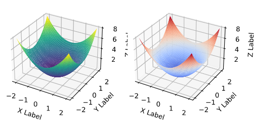
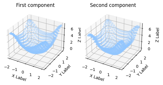
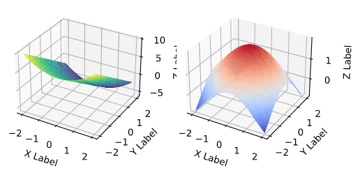
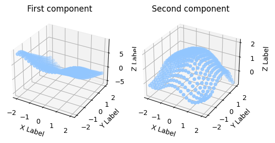
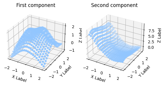
Figure 4: Simulation data: Left column shows the 3 of the true 8 functions (each from $[-2,2]\times[-2,2]\to\mathbb{R}^{2})$ while the right column gives the corresponding estimated clusters.

$\sigma$	$K$	log-lik	time
0.2	100	-174603.29	139.9
0.5	25	-45290.95	126.8
1	8	-29936.35	118.2
2	7	-36488.81	125.0
5	5	-51801.47	195.7

Table 1: Performance of Infinite HMM-GP on simulated data.

$\alpha$	$K$	time (3 iterations of MCMC)
0.2019	1	196.64

Table 2: Performance of DP-GP on simulated data.

To fit our model, we estimated the kernel parameters $\sigma_{0},\ell_{0}$ by using the GPy package on the data for the first time point. With $\alpha=\gamma=1$, we ran our algorithm in parallel for various values of $\sigma$. The results from various runs of the algorithm are shown in Table 1. Each row in the table shows for a particular $\sigma$, the number of clusters identified ($K$), the final log likelihood of the model (log-lik), and the time in seconds needed to run the algorithm (time). This is a sensible choice because not only are the correct number of clusters identified, the clusters’ posterior mean functions are similar to the functions used to generate the data. Table 1 also highlights the speed of the algorithm. The algorithm took around 2 minutes for this data set of 10,000 total observations.

Our experiments also demonstrate the inadequacy of DP-GP for this type of data, which underestimates the number of true clusters, and is time-consuming. Figure 1 in the appendix lists the true and estimated clusters for our model.

5.2 Velocity fields in an LA boulevard

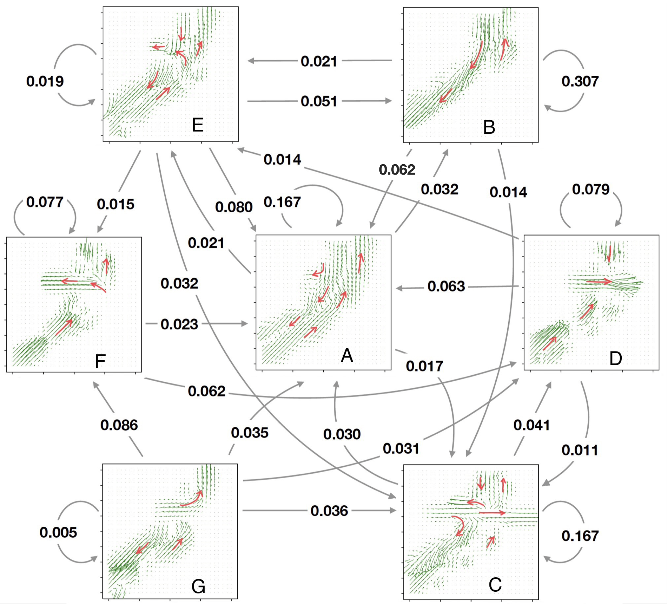
Figure 5: Some of the common states along with the estimated 20 step transition probabilities (each transition corresponds to a time gap of 10 seconds). While not generated by the algorithm, the red arrow marks are provided to easily visualize the traffic patterns.

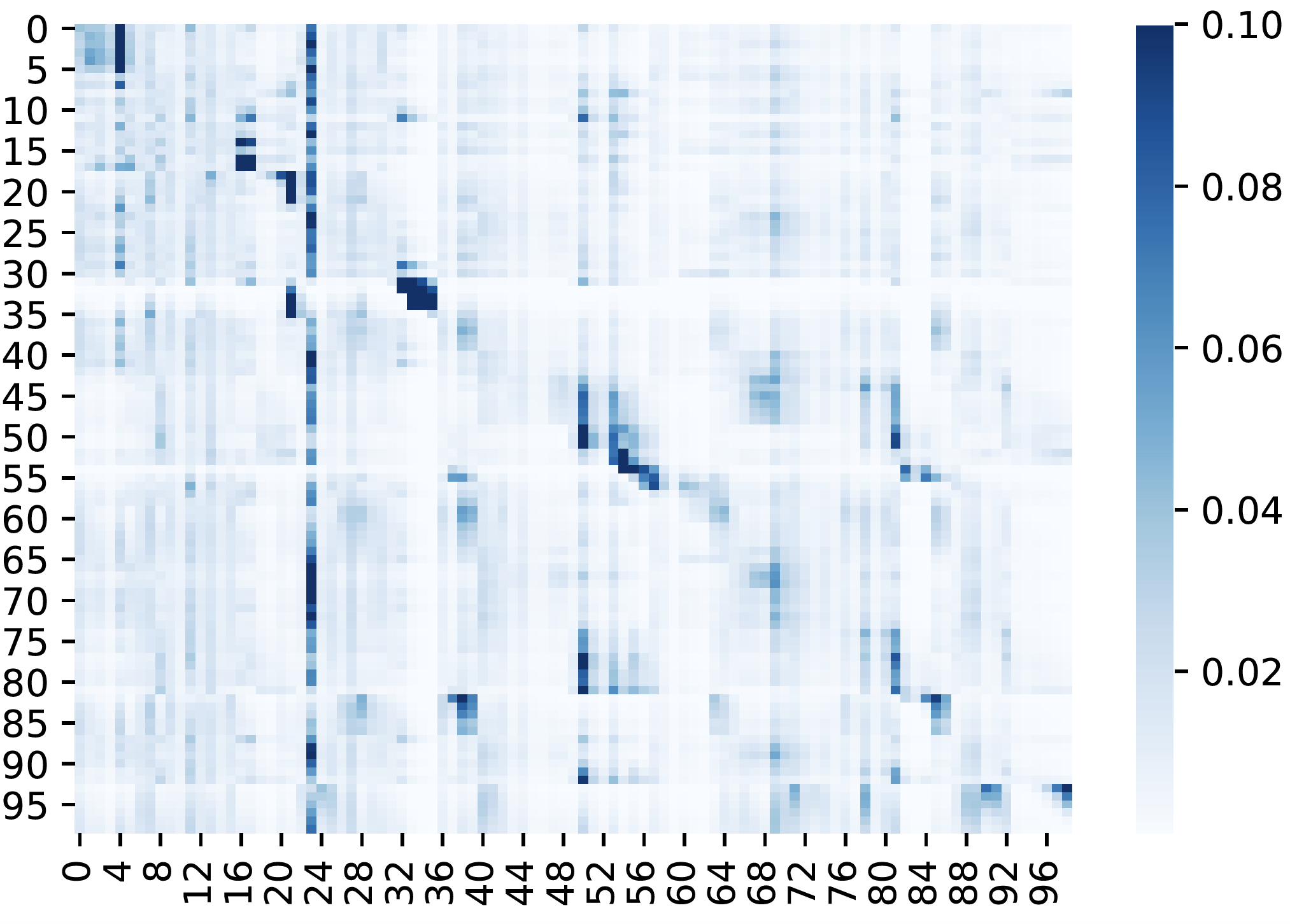
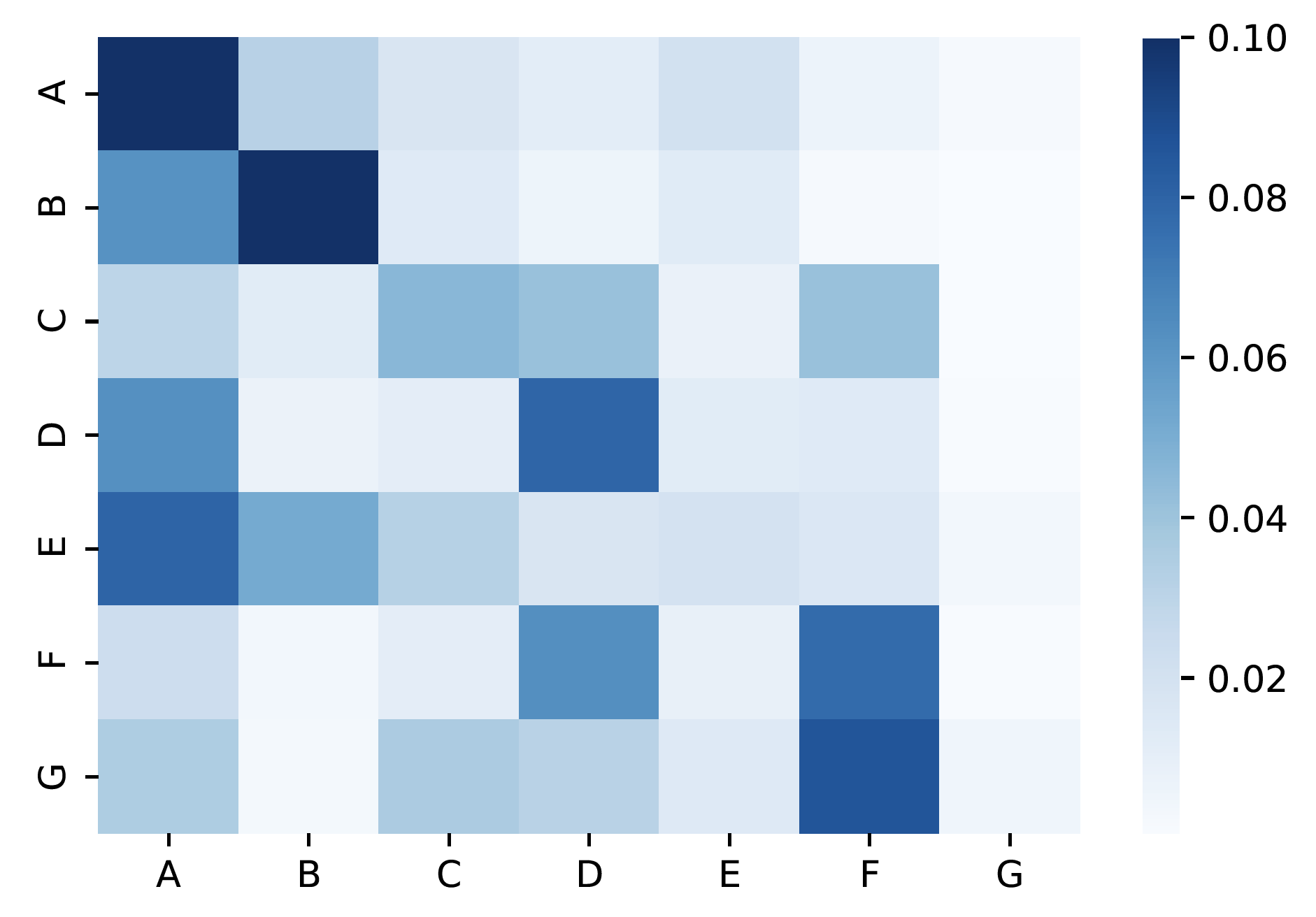
Figure 6: Heatmaps showing the estimated 20-step transition matrix for all hidden states in (a) and for the states considered in figure 6 in (b)

We chose a real-world traffic dataset collected as part of Federal Highway Administration’s (FWHA) Next Generation SIMulation (NGSIM) project. The dataset contains detailed multi-vehicle trajectories. As seen in Figure 1, we focused on data from the intersection of Lankershim Boulevard and Universal Hollywood Dr. in Los Angeles.

After scaling the region into a $[0,1]\times[0,1]$ box, we then discretized this data into frames with a duration of 0.5 seconds. Each frame contains the cars’ spatial location and velocity separated into the x and y component during that time period. For this study, we took $T=1000$ consecutive frames, which corresponds to roughly 8 minutes. We applied our model and algorithm to extract the latent traffic velocity spatial patterns while also studying the temporal dynamics.

We fixed the infinite HMM hyperparameters at $\alpha=1,\gamma=1$. After we tried different hyperparameters, we found that the log likelihood was highest when we set $\sigma=0.15$ and $\sigma_{0}=\ell_{0}=0.1$. Figure 6 shows the 7 most commonly occurring patterns that the algorithm identified with this choice of hyperparameters. These clusters are notated so A is the most frequent, B is the second most frequent, and so on. Interestingly enough, it appears that these patterns can be explained by the traffic lights at the intersections. For instance, there appears to be a green light on one or both sides of the vertical road in scenarios A, B, and E. In particular, scenario B differs from the other two because the green light is only for cars coming down the road. This figure also shows the importance of time dynamics. As seen by the moderate transition probabilities from E to C and from C to D and then moving to A, we can see that C is a transitional phase between patterns E (cars turning left from the main highway) and D (cars moving primarily left to right). Scenarios D and E cannot occur together.

It is also worth mentioning that some of the patterns discovered had a seemingly implausible traffic flow (towards the bottom right) and was later found that the data contained such apparent irregularities. However, upon careful inspection of the map, it was found that there is a driveway in that part of the road towards the right. This explains the apparent discrepancy because cars moving into the driveway would have a velocity directed towards the driveway. It further shows that such models can capture these subtle movements and patterns to give an unsupervised learning about the geography of the roads and the associated traffic patterns. On the other hand, the DP-GP identifies only 13 traffic patterns. It is exciting that we are able to extract such meaningful traffic patterns and understand the temporal dynamics in a fast efficient manner.

$\sigma_{0}=\ell_{0}$	$\sigma$	$K$	log-lik	time
0.1	0.1	166	-26461.12	3848.9
	0.15	99	-2790.70	4467.4
	0.2	66	-3878.23	5254.7
	0.25	41	-12989.42	7619.7
	0.3	32	-23212.65	9956.6

Table 3: Performance of Infinite-HMM-GP on the NGSIM data

$\alpha$	$K$	time ( 3 iterations)
1.8099	13	4460.7

Table 4: Performance of DP-GP on the NGSIM data

6 Conclusion

We propose a nonparametric framework to model the temporal and spatial aspects of traffic velocity vector field data via the use of Infinite HMM and Gaussian process. Additionally, we provide a fast, efficient sequential, one-pass algorithm for inference that performs MAP estimates of key variables at each step. The model allows us to have a better understanding of traffic movements and reveals interesting temporal patterns in traffic movement that are not captured by other nonparametric models. While the applications for this paper focuses primarily on traffic data, the techniques developed in the paper are also applicable to analyzing more generic spatio-temporal datasets in a fast, efficient manner.

Appendix A Computations for multivariate response data

A.1 Proof of proposition 4.1

Proof:

The proof of this proposition follows from the matrix normal assumption and the conditional normal formula. By the assumption we have

$$\begin{pmatrix}\text{vec}\left((x^{t^{j}_{k}})\mid_{k=1:j_{t}}\right)\\ \phi_{j}(z)\end{pmatrix}\,\sim\,\mathcal{N}_{d(N+1)}\Bigg{(}\boldsymbol{0},\begin{bmatrix}K_{x}&K_{x,\phi}\\ K_{x,\phi}^{T}&K_{\phi}\end{bmatrix}\Bigg{)},$$ (22)

where

$$K_{x}=K(Z_{t}^{j},Z_{t}^{j})\otimes\Omega(\rho)+I_{N}\otimes\sigma^{2}I_{d}$$

$$K_{x,\phi}=K(z,Z_{t}^{j})\otimes\Omega(\rho)$$

$$K_{\phi}=K(z,z)\otimes\Omega(\rho)$$

The proposition follows by using the formula for the conditional distribution of Gaussian random variable. The proposition can be easily extended to cover the case where we try to determine the posterior of $\phi_{j}$ at any $z_{1},\dots,z_{m}\in\mathbb{R}^{p}$, simply by vectorizing it and using the multivariate version of Lemma C.1 in section C.1.

$\square$

A.2 Update for state variable

second term in RHS of Eq.11:

Here, we provide the computation of the second term in the RHS of Eq.(11) in the main draft. Let $t^{j}_{1},\ldots,t^{j}_{j_{t}}\leq t$ denote all indices less than $t+1$ for which $s_{t}=j$. Then,

$$\operatorname{\mathbb{P}}(X_{t+1}(z^{t+1}_{1:n^{(t+1)}})\mid s_{t+1}=j,\mathcal{H}_{t})$$ (23)

$$= \int_{\Theta}F(X_{t+1}(z^{t+1}_{1:n^{(t+1)}});\phi_{j})dG(\phi|\{X_{u}:u\in T\})$$

$$= \operatorname{\mathbb{P}}(X_{t+1}(z^{t+1}_{1:n^{(t+1)}})\mid X_{t^{j}_{1}},\ldots,X_{t^{j}_{j_{t}}}).$$

Here, $G$ is the $MRGP(\mu,K,\rho)$ distribution. Moreover,

$$F(X_{t+1}(z^{t+1}_{1:n^{(t+1)}});\phi_{j})$$ (24)

$$= \operatorname{\mathbb{P}}(X_{t+1}(z^{t+1}_{1:n^{(t+1)}})\mid s_{t+1}=j,\{\phi_{k}\}).$$

The last line of Eq. (23) is then calculated using Prop. 4.1.

A.3 Update for oracle variable

Lemma A.1

$X_{t+1}(z^{t+1}_{1:n^{(t+1)}})$ is independent of $o_{t+1}$ conditioned on $s_{t+1}$, i.e.,

$$\operatorname{\mathbb{P}}(X_{t+1}(z^{t+1}_{1:n^{(t+1)}})\mid s_{t+1}=j,o_{t+1},\mathcal{H}_{t})$$ (25)

$$= \operatorname{\mathbb{P}}(X_{t+1}(z^{t+1}_{1:n^{(t+1)}})\mid s_{t+1}=j,\mathcal{H}_{t})$$

Proof:

First by Bayes’ Rule,

$$\operatorname{\mathbb{P}}(o_{t+1}=e\mid X_{t+1}(z^{t+1}_{1:n^{(t+1)}}),s_{t+1}=j,\mathcal{H}_{t})$$

$$\propto\operatorname{\mathbb{P}}(o_{t+1}=e\mid s_{t+1}=j,\mathcal{H}_{t})$$

$$\hskip 20.00003pt\operatorname{\mathbb{P}}(X_{t+1}(z^{t+1}_{1:n^{(t+1)}})\mid s_{t+1}=j,\mathcal{H}_{t})$$ (26)

Since $\operatorname{\mathbb{P}}(X_{t+1}(z^{t+1}_{1:n^{(t+1)}})\mid s_{t+1}=j,\mathcal{H}_{t})$ is free of $o_{t+1}$, it gets cancelled when normalized. Thus we obtain for every $j=\{1,\dots,\tilde{K}^{(t)}+1\}$ and $e\in\{0,1\}$,

$$\operatorname{\mathbb{P}}(o_{t+1}=e\mid X_{t+1}(z^{t+1}_{1:n^{(t+1)}}),s_{t+1}=j,\mathcal{H}_{t})$$ (27)

$$=\operatorname{\mathbb{P}}(o_{t+1}=e\mid s_{t+1}=j,\mathcal{H}_{t})$$

which reflects the fact that given $s_{t+1}$, $o_{t+1}$ does not depend on $X_{t+1}(z^{t+1}_{1:n^{(t+1)}})$. $\square$

Appendix B Prior literature

In this section we briefly introduce the various tools used in the paper.

B.1 Hierarchical Dirichlet Process

The HDP is a bayesian non parametric prior which enables us to fit mixture model for each group in a grouped data while allowing the mixtures to share components. Suppose there are $J$ groups, then HDP is a distribution over a set of random probability measures over $(\Theta,\mathcal{B})$; one $G_{j}$ for the $j$th group and a global probability measure $G_{0}$.

Suppose the $j$th group consists of $n_{j}$ datapoints $(x_{j1},\dots,x_{jn_{j}})$. The HDP model is as follows:

$$G_{0}|\gamma,H \sim DP(\gamma,H)$$ (28)

$$G_{j}|\alpha,G_{0} \sim DP(\alpha,G_{0})\quad,j=1,2\dots,J$$ (29)

$$\theta_{ji}|G_{j} \sim G_{j}\quad,j=1,2\dots,J$$ (30)

$$x_{ji}|\theta_{ji} \sim F(.|\theta_{ji})\quad,i=1,\dots,n_{j};j=1,\dots,J$$ (31)

The parameters include $\gamma$, $\alpha$ and $H$. $\theta$ are the latent factors in the model and $F$ is the kernel. $G_{j}$’s are conditionally independent given $G_{0}$ and given $G_{j}$, $\theta_{j1},\dots,\theta_{jn_{j}}$ are iid. To see how this model captures sharing of mixture components, we look at the stick breaking construction of the DP and find that $G_{0}$ is atomic and

$$G_{0}=\sum_{k}\beta_{k}\delta_{\phi_{k}}$$

Also, by construction of $G_{j}$,

$$G_{j}=\sum_{k}\pi_{jk}\delta_{\phi_{k}}$$

which shows that the atoms of $G_{j}$ originate from those of $G_{0}$ (and are hence shared across groups). Thus identifying $\phi_{k}$ as the parameter for the $k$th mixture component, we find that each of the $J$ groups are modelled as mixture distributions with the same set of (countably infinite) mixture components, but have different mixing proportions, given by $\pi_{j}=(\pi_{jk})_{k=1}^{\infty}$.

B.2 HDP-HMM

This is the model described in section (7) of (Teh et al., 2006). It uses the $\pi_{j}$ for both transitions and emissions.

As described in (3.1) in (Teh et al., 2006), the $\pi_{j}$ and the atoms $\theta_{k}$ can be generated equivalently as follows:

$$\beta|\gamma\sim GEM(\gamma)\quad\quad\pi_{j}|\alpha,\beta\sim DP(\alpha,\beta)\ \quad\theta_{k}|H\sim H$$

The $\pi_{j}=(\pi_{jk})_{k=1}^{\infty}$ denoted the mixture probabilities for the $j$th group over the atoms $\theta=(\theta_{k})_{k=1}^{\infty}$.

The model discussed in (7) in the same paper extends this to the HDP-HMM model which is as follows: there are countably infinite states (each representing a mixture) and all the mixtures share the same atoms/components. The hidden state indicates the component with transition given by the corresponding row of $\pi$ (now a doubly infinite stochastic matrix) and the emission is given as before. In particular, the model consists of the following (note $\beta$ is a probability distribution over $\mathbb{N}$)

$$\beta|\gamma \sim GEM(\gamma)$$

$$\pi_{k}|\alpha,\beta \sim DP(\alpha,\beta)$$

$$\theta_{k}|H \sim H$$

and the associated HMM is given by:

$$s_{t}|s_{t-1},\{\pi_{k}\}_{k=1}^{\infty} \sim\pi_{s_{t-1}}$$

$$x_{t}|s_{t},\{\theta_{k}\}_{k=1}^{\infty} \sim F(.|\theta_{s_{t}})$$

B.3 Matrix Normal Distribution

Let $X\in\mathbb{R}^{m\times n}$ be a random matrix valued random variable. We say that $X$ follows a matrix normal distribution ($MN_{mn}$ in short) with mean parameter $M\in\mathbb{R}^{m\times n}$ and scale parameters $U\in\mathbf{S}^{m}_{++}$ and $V\in\mathbf{S}^{n}_{++}$ if the pdf is

$$p(X|M,U,V)$$ (32)

$$= \frac{\exp\left(-\frac{1}{2}\text{tr}\left[(V^{-1}(X-M)^{T}U^{-1}(X-M)\right]\right)}{(2\pi)^{mn/2}|U|^{m/2}|V|^{n/2}}$$

We write this as

$$X\sim MN_{mn}(M,U,V)$$ (33)

$$\iff \text{vec}(X)\sim N_{mn}\left(\text{vec}(M),U\otimes V\right)$$

which establishes its connection with the multivariate normal distribution. Here vec indicates vectorized form of the corresponding matrix (we define it as vector obtained by stacking the rows of the matrix on top of each other) and $\otimes$ is the Kronecker product.

We list a few properties of this matrix normal distribution which follow readily using the equivalent multivariate normal form.

1. Mean: $\mathbb{E}(X)=M$

2. Second order moments:

   $$\mathbb{E}\left[(X-M)(X-M)^{T}\right]=U\text{tr}(V),$$

   $$\mathbb{E}\left[(X-M)^{T}(X-M)\right]=V\text{tr}(U)$$

3. For appropriate sized matrices $A,B,C$ we have

   $$\mathbb{E}\left[XAX^{T}\right] =U\text{tr}(A^{T}V)+MAM^{T}$$

   $$\mathbb{E}\left[X^{T}BX\right] =V\text{tr}(UB^{T})+M^{T}BM$$

   $$\mathbb{E}\left[XCX\right] =VC^{T}U+MCM$$

4. If $X\sim MN_{mn}(M,U,V)$ then

   $$X^{T} \sim MN_{nm}(M^{T},V,U)$$

   $$DXC \sim MN_{rs}(DMC,DUD^{T},C^{T}VC)$$

   where$D\in\mathbb{R}^{r\times m}$ has rank $r\leq m$ and $C\in\mathbb{R}^{n\times s}$ has rank $s\leq n$.

5. Maximum likelihood estimation: Let $X_{1},\dots,X_{k}\overset{iid}{\sim}MN_{mn}(M,U,V)$, then the MLE of $M$ has a closed form solution:

   $$\hat{M}=\frac{1}{k}\sum_{j=1}^{k}X_{k}$$

   However $U$ and $V$ do not have MLE in closed form but they satisfy:

   $$U =\frac{1}{kn}\sum_{j=1}^{k}(X_{j}-M)V^{-1}(X_{j}-M)^{T}$$

   $$V =\frac{1}{km}\sum_{j=1}^{k}(X_{j}-M)^{T}U^{-1}(X_{j}-M)$$

   The estimates are positive definite if $k\geq\max\{m/n,n/m\}+1$. Also they are identifiable upto a scalar multiple, i.e. $MN_{mn}(M,U,V)=MN_{mn}(M,sU,(1/s)V)$

Appendix C Calculations for posterior computation

In this section we consider the calculations for univariate response data. The results for the multivariate case follow similarly.

C.1 Univariate response data

Consider the case of univariate response data. i.e. every cluster is a function $\phi_{j}:\mathbb{R}^{p}\to\mathbb{R}$ and we place a usual Gaussian process prior on them. We also consider isotropic data in this section, i.e. for each time point we observe noisy observations around the true cluster functions at the same spatial locations $z_{1},\dots,z_{N}\in\mathbb{R}^{p}$. We describe computing the posterior predictive distribution of $\phi_{k}$ at time $t+1$ for some $t\in{1,2\ldots,T}$, $k\in{1,2,\ldots,K^{(t)}}$, and $N\in\mathbbm{N}$.

Recall that given $s_{t}=j$, the observation at time $t$ are given by

$$X_{t}(z_{i})=\phi_{j}(z_{i})+\epsilon_{ji},$$ (34)

$i=1,\dots,N$ and $\epsilon$’s are iid $\mathcal{N}(0,\sigma^{2})$. The posterior computation for the latent function, $\phi_{j}$ can be obtained by the following lemma.

Lemma C.1

Let $t_{1},t_{2},\ldots,t_{N_{k}^{(t)}}$, $N_{k}^{(t)}\in\mathbbm{N}$, indicate the times during which $\widehat{s}_{t^{\prime}}=k$ for $t^{\prime}\leq t$. Let us define $X_{t}=(X_{t}(z_{1}),\dots,X_{t}(z_{N}))^{T}\in\mathbb{R}^{N}$, $z=(z_{1},\dots,z_{N})$ and $\phi_{k}(z)=(\phi_{k}(z_{1}),\dots,\phi_{k}(z_{N}))^{T}$. Moreover, let $K$ be the $N\times N$ RBF kernel matrix over $(z_{1},\dots,z_{N})$, i.e. $K_{ij}=K(z_{i},z_{j})$ for $i,j\in\{1,\dots,N\}$. Then, the posterior of $\phi$ conditioned on the data is given by:

$$\phi_{k}(z) |X_{t_{1}},X_{t_{2}},\ldots,X_{t_{N_{k}^{(t)}}}\sim$$ (35)

$$\mathcal{N}_{N}\Big{(}K_{x,\phi}^{T}K_{x}^{-1}\boldsymbol{x},K_{\phi}-K_{x,\phi}^{T}K_{x}^{-1}K_{x,\phi}\Big{)}.$$

where $\boldsymbol{x}$ is the $NN_{k}^{(t)}$ length vector obtained by stacking $X_{t_{1}},\dots,X_{t_{N_{k}^{(t)}}}$ and

$$K_{\phi}=K,\quad K_{x,\phi}=\begin{bmatrix}K\\ \vdots\\ K\end{bmatrix}_{NN^{(t)}_{k}\times N},$$

$$K_{x}=\begin{bmatrix}K+\sigma^{2}I&K&\dots&K\\ K&K+\sigma^{2}I&\dots&K\\ \vdots&\vdots&\ddots&\vdots\\ K&K&\dots&K+\sigma^{2}I\end{bmatrix}_{NN^{(t)}_{k}\times NN^{(t)}_{k}}.$$

Moreover,

$$X_{t} |\hat{s}_{t}=k,\mathcal{H}_{t-1}\sim$$ (36)

$$\mathcal{N}_{N}\Big{(}K_{x,\phi}^{T}K_{x}^{-1}\boldsymbol{x},K_{\phi}-K_{x,\phi}^{T}K_{x}^{-1}K_{x,\phi}+\sigma^{2}I_{N}\Big{)}.$$

Proof:

By normality, we have that

$$\begin{pmatrix}X_{t_{1}}\\ X_{t_{2}}\\ \vdots\\ X_{t_{N_{k}^{(t)}}}\\ \phi_{k}(z)\end{pmatrix}\,\sim\,\mathcal{N}_{N(N_{k}^{(t)}+1)}\Bigg{(}\boldsymbol{0},\begin{bmatrix}K_{x}&K_{x,\phi}\\ K_{x,\phi}^{T}&K_{\phi}\end{bmatrix}\Bigg{)},$$

The result now follows by using the formulation of the conditional normal distribution. The proof of Eq. (36) also follows similarly. $\square$

Notice that the kernel $K$ stays the same for every time point because $z_{1},\dots,z_{N}$ are fixed in this case.

The inversion of matrix $K_{x}$ is computationally intensive as $K_{x}$ is $NN^{(t)}_{k}\times NN^{(t)}_{k}$. Moreover, $K_{x}$, which is $NN^{(t)}_{k}\times NN^{(t)}_{k}$ and grows as new points are included. Therefore, to circumvent the issue of inverting the matrix, we can instead use the spectral decomposition of $K$. This method is described in the following lemma.

Lemma C.2

Suppose that $K$ has eigenvalues $\lambda_{1},\lambda_{2},\ldots,\lambda_{N}$ with corresponding eigenvectors $v_{1},v_{2},\ldots,v_{N}\in\mathbbm{R}^{N}$. For $U\in\mathbbm{R}^{NN^{(t)}_{k}\times N}$, let $U=[u_{1},u_{2},\ldots,u_{N^{(t)}_{k}}]$ where $u_{n}=\mathbf{1}_{N^{(t)}_{k}}\otimes v_{n}/\sqrt{N^{(t)}_{k}}$, $n=1,2,\ldots,N$. Set $D$ to be a diagonal $N\times N$ matrix such that the $n$th diagonal entry is given by $-\frac{k\lambda_{i}}{\sigma^{2}(k\lambda_{i}+\sigma^{2})}$. Then,

$$K_{x}^{-1}=UDU^{T}+\frac{1}{\sigma^{2}}I_{NN^{(t)}_{k}}.$$ (37)

Proof:

We use the following result corresponding to Kronecker product (Theorem 4.2.12 in (Horn et al., 1994)) to ease this computation.

Theorem C.1 (Eigendecomposition: Kronecker Product)

Suppose $A\in\mathbb{M}^{n}$ and $B\in\mathbb{M}^{m}$. Let $\lambda$ be an eigenvalue of $A$ with corresponding eigenvector $x$ and $\mu$ be an eigenvalue of $B$ with corresponding eigenvector $y$. Then $\lambda\mu$ is an eigenvalue of $A\otimes B$ with corresponding eigenvector $x\otimes y$. Any eigenvalue of $A\otimes B$ arises as such a product of eigenvalues of A and B.

Recall that $K_{x}=A+\sigma^{2}I$ where $A=\boldsymbol{1}_{N^{(t)}_{k}}\boldsymbol{1}_{N^{(t)}_{k}}^{T}\otimes K$.

Step 1: We first provide the eigendecomposition of $K_{x}$.

Consider the eigendecomposition of $A$.

Let $K=\sum_{i=1}^{N}\lambda_{i}v_{i}v_{i}^{T}$ be the eigendecomposition of $K$ (note that $K$ is fixed throughout and this decomposition needs to be done once).

Also, $\boldsymbol{1}_{N^{(t)}_{k}}\boldsymbol{1}_{N^{(t)}_{k}}^{T}=N^{(t)}_{k}\frac{\boldsymbol{1}_{N^{(t)}_{k}}}{\sqrt{N^{(t)}_{k}}}\frac{\boldsymbol{1}_{N^{(t)}_{k}}}{\sqrt{N^{(t)}_{k}}}^{T}$ gives the corresponding decomposition for $\boldsymbol{1}_{N^{(t)}_{k}}\boldsymbol{1}_{N^{(t)}_{k}}^{T}$.

Thus the eigendecomposition of $A$ by Lemma C.1 is

$$A=\sum_{i=1}^{N}(N^{(t)}_{k}\lambda_{i})u_{i}u_{i}^{T}\quad\text{where }u_{i}=\boldsymbol{1}_{N^{(t)}_{k}}\otimes v_{i}/\sqrt{N^{(t)}_{k}}$$

showing that $A$ has only $N$ non-zero eigenvalues with corresponding eigenvectors $u_{1},\dots,u_{N}$.

Now extend $\{u_{1},\dots,u_{N}\}$ to an orthonormal basis of $\mathbb{R}^{NN^{(t)}_{k}}$, as $\{u_{1},\dots,u_{N},u_{N+1},\dots,u_{NN^{(t)}_{k}})$ (e.g. Gram Schmidt).

Then we can write $K_{x}$ as

$$K_{x} = A+\sigma^{2}I=\sum_{i=1}^{N}(N^{(t)}_{k}\lambda_{i})u_{i}u_{i}^{T}+\sum_{j=1}^{NN^{(t)}_{k}}\sigma^{2}u_{j}u_{j}^{T}$$ (38)

$$= \sum_{i=1}^{N}(N^{(t)}_{k}\lambda_{i}+\sigma^{2})u_{i}u_{i}^{T}+\sum_{i>N}\sigma^{2}u_{i}u_{i}^{T}$$

which shows that $K_{x}$ has eigenvalues $N^{(t)}_{k}\lambda_{1}+\sigma^{2},\dots,N^{(t)}_{k}\lambda_{N}+\sigma^{2}$ with multiplicity 1 and $\sigma^{2}$ with multiplicity $NN^{(t)}_{k}-N$.

Step 2: From the eigendecomposition of $K_{x}$, the decomposition for $K_{x}^{-1}$ is given by

$$K_{x}^{-1} =\sum_{i=1}^{N}\frac{1}{N^{(t)}_{k}\lambda_{i}+\sigma^{2}}u_{i}u_{i}^{T}+\sum_{i>N}\frac{1}{\sigma^{2}}u_{i}u_{i}^{T}$$

$$=\sum_{i=1}^{N}\Bigg{(}\frac{1}{N^{(t)}_{k}\lambda_{i}+\sigma^{2}}-\frac{1}{\sigma^{2}}\Bigg{)}u_{i}u_{i}^{T}+\frac{1}{\sigma^{2}}I_{NN^{(t)}_{k}}$$

$$=-\frac{1}{\sigma^{2}}\sum_{i=1}^{N}\Bigg{(}\frac{N^{(t)}_{k}\lambda_{i}}{N^{(t)}_{k}\lambda_{i}+\sigma^{2}}\Bigg{)}u_{i}u_{i}^{T}+\frac{1}{\sigma^{2}}I_{NN^{(t)}_{k}}$$ (39)

The first term can be written as $UDU^{T}$, where,

$$D=\frac{1}{\sigma^{2}}\begin{bmatrix}-\frac{N^{(t)}_{k}\lambda_{1}}{N^{(t)}_{k}\lambda_{1}+\sigma^{2}}&0&\dots&0\\ 0&-\frac{N^{(t)}_{k}\lambda_{2}}{N^{(t)}_{k}\lambda_{2}+\sigma^{2}}&\dots&0\\ \vdots&\vdots&\ddots&\vdots\\ 0&0&\dots&-\frac{N^{(t)}_{k}\lambda_{n}}{N^{(t)}_{k}\lambda_{n}+\sigma^{2}}\end{bmatrix}$$

This proves the result. $\square$

During initialization, we spectral decompose $K$ to get $\lambda_{1},\dots,\lambda_{N}$ and $v_{1},\dots,v_{N}$ and store them. Then, when needed as in our discussion above, we construct the $NN^{(t)}_{k}\times N$ matrix $U=\begin{bmatrix}u_{1}&u_{2}&\dots&u_{N}\end{bmatrix}$ and a $N\times N$ diagonal matrix $D$ and then use $K_{x}^{-1}=UDU^{T}+\frac{1}{\sigma^{2}}I_{NN^{(t)}_{k}}$ to get the required inverse.

Note that we can further speed up computation using the above decomposition because we only have to compute the eigenvalues of $K$ once. $K_{x}$ is a $NN^{(t)}_{k}\times NN^{(t)}_{k}$ matrix and its Cholesky decomposition has complexity $O(N^{3}(N^{(t)}_{k})^{3}/3)$, which is quite large for $N^{(t)}_{k}\approx 10^{4}$ and $N\approx 100$ and considering that we need to do this for every time point $t$.

C.2 Multivariate response case

C.2.1 Efficient matrix inversion for the multivariate case

The target is to update the matrix

$$\Lambda^{(t)}=\left(K(Z_{k}^{t},Z_{k}^{t})\otimes\Omega(\rho)+\sigma^{2}I_{Nd}\right)^{-1}$$

in an online manner.

Recall that this is required for the computing the posterior predictive distribution for the $k$th cluster at every time point but we only need to invert this afresh every time some new data is assigned to this cluster. We assume that the dimension of the data is fixed whereas the number of total data points increases each time new data is given.

Our approach is the following. At the first time some data is given to $\phi_{k}$, we estimate $\rho$ using the method discussed in the previous section. Denote this estimate as $\rho^{(1)}$. If $K^{(1)}$ represents the RBF kernel of the GP over $Z_{k}^{1}$, we set $\Lambda^{(1)}$ so that

$$\Lambda^{(1)}=\left(K^{(1)}\otimes\Omega(\rho^{(1)})+\sigma^{2}I_{n_{1}d}\right)^{-1}.$$

Now suppose we assign new data to this cluster at times $t_{1},\dots,t_{N_{k}^{(t)}}$ and each time we compute $\Lambda^{(1)},\dots,\Lambda^{(N_{k}^{(t)})}$ (each time saving the last matrix). Now let at some later time point, $t^{\prime}$, some new data is given to $\phi_{k}$. We have saved $\rho^{(N_{k}^{(t)})}$ and $\Lambda^{(N_{k}^{(t)})}$. Then, we again first use the new data to estimate $\rho^{(N_{k}^{(t)}+1)}$. Let $K(Z_{t}^{k},Z_{t}^{k})$ denote the RBF kernel with the old data till $t$, $K(z^{(t^{\prime})},z^{(t^{\prime})})$ represent the RBF kernel with the new data at $t^{\prime}$, and $K(Z_{t}^{k},z^{(t^{\prime})})$ designate the RBF kernel computed between the old and new data. Also write $N=\sum_{s\leq N_{k}^{(t)}}n^{(t_{s})}$ be the total number of data points associated with this cluster till time $t$. We can then write

$$\left(\Lambda^{(N_{k}^{(t)}+1)}\right)^{-1}=\begin{bmatrix}A_{11}&A_{12}\\ A_{21}&A_{22}\end{bmatrix},$$ (40)

where

$$A_{11} =K(Z_{t}^{k},Z_{t}^{k})\otimes\Omega(\rho^{(N_{k}^{(t)}-1)})+\sigma^{2}I_{Nd},$$

$$A_{12} =K(Z_{t}^{k},z^{(t^{\prime})})\otimes\Omega(\rho^{(N_{k}^{(t)})}),$$

$$A_{21} =A_{12}^{T},$$

$$A_{22} =K(z^{(t^{\prime})},z^{(t^{\prime})})\otimes\Omega(\rho^{(t^{\prime})})+\sigma^{2}I_{n^{(t^{\prime})}d}.$$

Using the matrix inverse for block matrix, we have that

$$\Lambda^{(N_{k}^{(t)}+1)}=\begin{bmatrix}\Lambda^{(N_{k}^{(t)}+1)}_{11}&\Lambda^{(N_{k}^{(t)}+1)}_{12}\\ \Lambda^{(N_{k}^{(t)}+1)}_{21}&\Lambda^{(N_{k}^{(t)}+1)}_{22}\end{bmatrix}$$ (41)

with

$$\Lambda^{(N_{k}^{(t)}+1)}_{11} =A_{11}^{-1}+A_{11}^{-1}A_{12}\Lambda^{(N_{k}^{(t)}+1)}_{22}A_{21}A_{11}^{-1},$$

$$\Lambda^{(N_{k}^{(t)}+1)}_{12} =-A_{11}^{-1}A_{12}\Lambda^{(N_{k}^{(t)}+1)}_{22},$$

$$\Lambda^{(N_{k}^{(t)}+1)}_{21} =-\Lambda^{(2)}_{22}A_{21}A_{11}^{-1},$$

$$\Lambda^{(N_{k}^{(t)}+1)}_{22} =\left(A_{22}-A_{21}A_{11}^{-1}A_{12}\right)^{-1}.$$

While we now need two inverses to compute $\Lambda^{(N_{k}^{(t)}+1)}$, updating it in this manner is computationally faster. We have already calculated $A_{11}^{-1}$ because $A_{11}^{-1}=\Lambda^{(N_{k}^{(t)})}$. Further, the other inverse is the inverse of a $n^{(t^{\prime})}d\times n^{(t^{\prime})}d$ matrix. As more data is added to a GP, it will be much faster to invert such a matrix compared to the matrix in (40) as a whole which has dimensions of $(N+n^{(t^{\prime})})d\times(N+n^{(t^{\prime})})d$.

C.2.2 Estimating $\rho$

We apply a moment-matching approach to find a suitable plug-in estimator of $\rho$ for $\phi_{j}$ at time $t$. If $\bar{X}_{t}=\frac{1}{N^{(t)}_{k}}\sum_{t^{\prime}=t_{1},t_{2},\ldots,t_{T_{k}}}X_{t^{\prime}}$, our goal is to match the second moment from the MRGP assumption to $\frac{1}{Nd}(X_{t}-\bar{X}_{t})(X_{t}-\bar{X}_{t})^{T}$. Due to the form of $\Omega(\rho)$, we have after some rearrangement that $\rho A=B$ where

$$A =\left[K\otimes\mathbf{1}_{d}\mathbf{1}_{d}^{T}-K\otimes I_{d}\right]$$

$$B =\frac{1}{Nd}(X_{t}-\bar{X}_{t})(X_{t}-\bar{X}_{t})^{T}-\sigma^{2}I_{Nd}-K\otimes I_{d}.$$

Here $K=K(Z_{t}^{j},Z_{t}^{j})$ is the $N\times N$ covariance kernel over all the spatial locations associated to cluster $j$ till time $t$. We then choose our estimator, $\widehat{\rho}$, so as to minimize $\left\lVert\rho A-B\right\rVert_{F}$. This has the following closed form solution:

$$\widehat{\rho}=\frac{\sum_{i,j}A_{ij}B_{ij}}{\sum_{i,j}A_{ij}^{2}}$$ (42)

Appendix D Experiments

This section contains additional experimental results. Figure 7 provides an illustration of the transition matrix for the NGSIM data. The transition matrix reflects the natural intuition that traffic flows tend to stay in the same state over a short duration of time. This is reflective of the fact that traffic lights may control the flow of traffic for a certain duration of time and then as traffic light directions change, so does the traffic flow pattern. On the other hand, movement patterns are quite flexible over large durations as shown by the 60-step transition matrix.

Figure 8 shows the 8 true functions(on the left) that were used for the purpose of simulations along with their data estimates (on the right). By simple eyeballing, the estimates look to match the true functions closely.

Table 5 provides results with NGSIM data for various parameter settings with infinite HMM-GP.

$\sigma_{0}=\ell_{0}$	$\sigma$	$K$	log-lik	time
0.07	0.1	109	-31487.76	5299.7
	0.15	64	-13808.98	7093.2
	0.2	41	-15939.11	10885.7
	0.25	29	-21262.44	18023.6
	0.3	20	-27805.92	22157.2
0.1	0.1	166	-26461.12	3848.9
	0.15	99	-2790.70	4467.4
	0.2	66	-3878.23	5254.7
	0.25	41	-12989.42	7619.7
	0.3	32	-23212.65	9956.6
0.3	0.1	343	-127120.84	5112.8
	0.15	213	-42825.24	4734.9
	0.2	138	-25478.42	5775.6
	0.25	96	-23204.13	6972.8
	0.3	74	-28864.42	8752.1

Table 5: Table showing performance of our algorithm on the NGSIM data. The hyperparameters with the highest log likelihood is bolded.

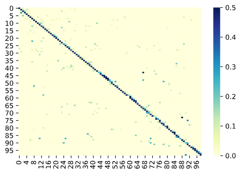
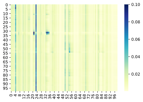
Figure 7: Heatmaps showing the estimated 1-step transition matrix for all hidden states in (a) and 60-step in (b)

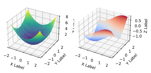
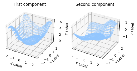
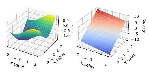
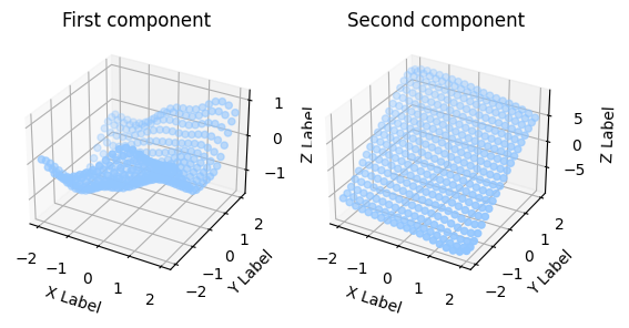
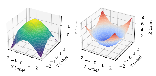
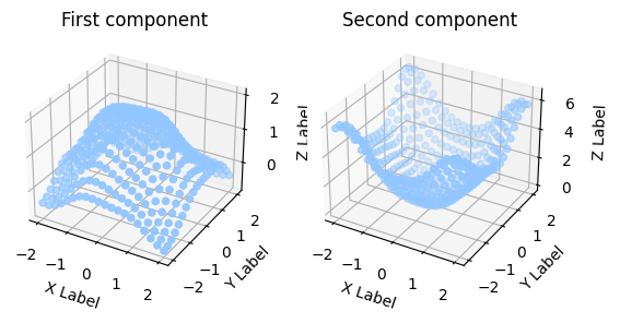
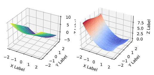
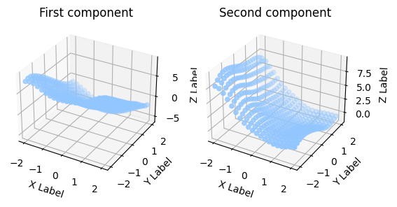
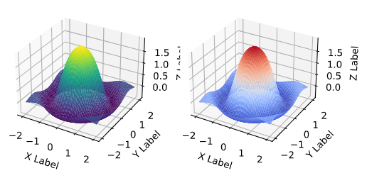
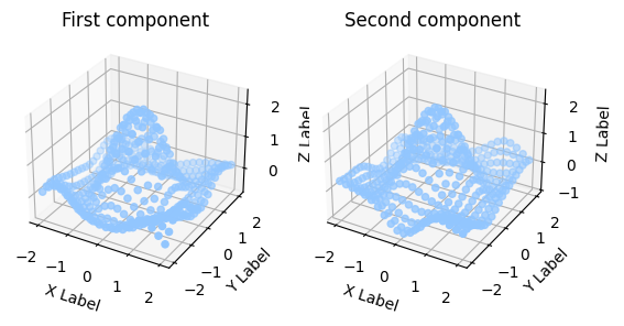
Figure 8: Simulation data: Left column shows the true 8 functions (each from $[-2,2]\times[-2,2]\to\mathbb{R}^{2})$ while the right column gives the 8 estimated clusters

References

• Antoniak (1974) Antoniak, C. Mixtures of dirichlet processes with applications to bayesian nonparametric problems. Annals of Statistics, 2(6):1152––1174, 1974.
• Beal et al. (2002) Beal, M. J., Ghahramani, Z., and Rasmussen, C. E. The infinite hidden markov model. In Advances in neural information processing systems, pp. 577–584, 2002.
• Blei & Jordan (2006) Blei, D. and Jordan, M. Variational inference for dirichlet process mixtures. Bayesian Analysis, 1:121–144, 2006.
• Blei et al. (2003) Blei, D., Ng, A., and Jordan, M. Latent Dirichlet allocation. J. Mach. Learn. Res, 3:993–1022, 2003.
• Chen et al. (2016) Chen, Y. F., Liu, M., Liu, S., Miller, J., and How, J. Predictive modeling of pedestrian motion patterns with bayesian nonparametrics. AIAA 2016-1861, 2016.
• Cressie (1993) Cressie, N. Statistics for Spatial Data. Wiley, NY, 1993.
• Ferguson (1973) Ferguson, T. A Bayesian analysis of some nonparametric problems. Ann. Statist., 1:209–230, 1973.
• (8) Foti, N., Xu, J., Laird, D., and Fox, E. B. Stochastic variational inference for hidden markov models.
• Fox et al. (2009) Fox, E., Sudderth, E., Jordan, M. I., and Willsky, A. The sticky hdp-hmm: Bayesian nonparametric hidden Markov models with persistent states. Technical Report P-2777, MIT LIDS, 2009.
• Fox et al. (2011) Fox, E. B., Sudderth, E. B., Jordan, M. I., and Willsky, A. S. A sticky hdp-hmm with application to speaker diarization. Annals of Applied Statistics, 5 : 2A:1020–1056, 2011.
• Gelfand & Smith (1990) Gelfand, A. and Smith, A. Sampling-based approaches to calculating marginal densities. Journal of the American Statistical Association, 85 (410):398–409, 1990.
• Ghosal & van der Vaart (2017) Ghosal, S. and van der Vaart, A. Fundamentals of nonparametric Bayesian inference, vol. 44 of Cambridge Series in Statistical and Probabilistic Mathematics. Cambridge University Press, Cambridge, 2017.
• Guo et al. (2019) Guo, Y., Kalidindi, V. V., Arief, M., Wang, W., Zhu, J., Peng, H., and Zhao, D. Modeling multi-vehicle interaction scenarios using gaussian random field. arXiv preprint arXiv:1906.10307, 2019.
• Hoffman et al. (2013) Hoffman, M. D., Blei, D. M., Wang, C., and Paisley, J. Stochastic variational inference. Journal of Machine Learning Research, 14(1):1303–1347, May 2013.
• Horn et al. (1994) Horn, R. A., Horn, R. A., and Johnson, C. R. Topics in matrix analysis. Cambridge university press, 1994.
• Jordan et al. (1999) Jordan, M. I., Ghahramani, Z., Jaakkola, T. S., and Saul, L. K. An introduction to variational methods for graphical models. Machine Learning, 37(2):183–233, 1999.
• Joseph et al. (2011) Joseph, J., Doshi-Velez, F., Huang, A. S., and Roy, N. A bayesian nonparametric approach to modeling motion patterns. Autonomous Robots, 31(4):383, 2011.
• Kim et al. (2011) Kim, K., Lee, D., and Essa, I. Gaussian process regression flow for analysis of motion trajectories. In Proceedings of IEEE International Conference on Computer Vision (ICCV). IEEE Computer Society, November 2011.
• Mandt et al. (2017) Mandt, S., Hoffman, M. D., and Blei, D. M. Stochastic gradient descent as approximate Bayesian inference. Journal of Machine Learning Research, 18(134):1–35, 2017.
• Rabiner (1989) Rabiner, L. A tutorial on hidden markov models and selected applications in speech recognition. Proceedings of the IEEE, 77:257––285, 1989.
• Teh et al. (2006) Teh, Y., Jordan, M., Beal, M., and Blei, D. Hierarchical Dirichlet processes. J. Amer. Statist. Assoc., 101:1566–1581, 2006.