Riemann zeros from a periodically-driven trapped ion

Abstract

The non-trivial zeros of the Riemann zeta function are central objects in number theory. In particular, they enable one to reproduce the prime numbers. They have also attracted the attention of physicists working in Random Matrix Theory and Quantum Chaos for decades. Here we present an experimental observation of the lowest non-trivial Riemann zeros by using a trapped ion qubit in a Paul trap, periodically driven with microwave fields. The waveform of the driving is engineered such that the dynamics of the ion is frozen when the driving parameters coincide with a zero of the real component of the zeta function. Scanning over the driving amplitude thus enables the locations of the Riemann zeros to be measured experimentally to a high degree of accuracy, providing a physical embodiment of these fascinating mathematical objects in the quantum realm.

I Main

The Riemann zeta function $\zeta(s)$ is the Rosseta stone for number theory. The stone, found by Napoleon’s troops in Egypt, contains the same text written in three different languages, which enabled the Egyptian hieroglyphics to be deciphered. The $\zeta$-function is also expressed in three different “languages”: as the series $\sum_{n}n^{-s}$ over the positive integers $n$, as the product $\prod_{p}1/(1-p^{-s})$ over the prime numbers $p$, and as the product $\propto\prod_{n}(1-s/\rho_{n})e^{s/\rho_{n}}$ over the Riemann zeros $\rho_{n}$ edwards . Riemann conjectured in 1859 that these zeros would have a real part equal to a half, $\rho_{n}=\frac{1}{2}+iE_{n}$, where $E_{n}$ is a real number riemann . This is the famous Riemann Hypothesis (RH), one of the six unsolved Millennium problems, whose solution would amplify our knowledge of the distribution of prime numbers with resulting consequences for number theory and factorization schemes millennium ; conrey . More poetically, in the words of M. Berry, the proof of the RH would mean that there is music in the prime numbers music .

One of the most interesting ideas to attack the RH is to show that the $E_{n}$ are the eigenvalues of the Hamiltonian of a quantum system. This idea, suggested by Pólya and Hilbert around 1912 montgomery73 , began to be taken seriously in the 70s with Montgomery’s observation montgomery75 that the Riemann zeros closely satisfy the statistics of the Gaussian unitary ensemble (GUE). In the 80s Odlyzko odlyzko tested this prediction numerically for $10^{5}$ zeros around the $10^{20}$th zero, finding only minor deviations from the GUE. These were explained later by Berry and collaborators berry86 ; berry88 ; BK96 using the theory of quantum chaos, and led him to propose that the $E_{n}$ are the eigenvalues of a quantum chaotic Hamiltonian whose classical version contains isolated periodic orbits whose periods are the logarithm of the prime numbers. Much work has been done BK99 -S19 to find such a Hamiltonian, but so far without a definitive answer.

In this Letter we present an experimental observation of the lowest Riemann zeros, which is quite different from the spectral realization described above. Our intention is not to prove the RH, but rather to provide a physical embodiment of these mathematical objects by using advanced quantum technology. The physical system that we consider is a trapped-ion qubit. The ion is subjected to a time-periodic driving field, and consequently its behaviour is described by Floquet theory, in which the familiar energy eigenvalues of static quantum systems are generalized to “quasienergies”. These quasienergies can be regulated by the parameters of the driving, in a technique termed Floquet engineering. In particular, when the quasienergies are degenerate (or cross) the ion’s dynamics is frozen, which can be observed experimentally. The Riemann zeta function enters into this construction in the design of the driving field, which is engineered to produce the freezing of the dynamics when the real part of $\zeta(s)/s$, with $s=\frac{1}{2}+iE$, vanishes. Thus observing the freezing of the qubit’s dynamics as the driving parameters are varied gives a high-precision experimental measurement of the location of the Riemann zeros.

I.1 Floquet theory

We consider a two-level system subjected to a time-periodic driving, described by the Hamiltonian $H(t)=J\left(\sigma_{x}+\frac{f(t)}{2}\sigma_{z}\right)$, where $\sigma_{x,z}$ are the standard Pauli matrices and $J$ represents the bare tunneling between the two energy levels. Henceforth we will set $\hbar=1$, and measure all energies (times) in units of $J$ ($J^{-1}$). As $H(t)$ is time-periodic, $H(t)=H(t+T)$, where $T$ is the period of the driving, the system is naturally described within Floquet theory, using a basis of Floquet modes and quasienergies which can be extracted from the unitary time-evolution operator for one driving-period $U=\mathcal{T}\mathrm{exp}\left[-i\int_{0}^{T}H(t^{\prime})dt^{\prime}\right]$ (where $\mathcal{T}$ denotes the time-ordering operator). The Floquet modes, $|\Phi_{j}(t)\rangle$, are the eigenstates of $U$, and the quasienergies, $\epsilon_{j}$, are related to the eigenvalues of $U$ via $\lambda_{j}=\mathrm{exp}\left[-iT\epsilon_{j}\right]$.

The Floquet modes provide a complete basis to describe the time-evolution of the system, and the quasienergies play an analogous role to the energy eigenvalues of a time-independent system. The state of the qubit can thus be expressed as $|\psi(t)\rangle=\sum_{j}\alpha_{j}\mathrm{exp}\left[-i\epsilon_{j}t\right]|\Phi_{j}(t)\rangle$, where the expansion coefficients $\alpha_{j}$ are time-independent, and the Floquet modes are $T$-periodic functions of time. From this expression, it is clear that if two quasienergies approach degeneracy, the timescale for tunneling between them will diverge as $1/\Delta\epsilon$. Although in general it is difficult to obtain explicit forms for the quasienergies, even for the case of a two-level system, excellent approximations can be obtained in the high-frequency limit, when $\Omega=2\pi/T$ is the largest energy scale of the problem, that is, $\Omega\gg J$. In that case one can derive cec_prb an effective static Hamiltonian, $H_{\mathrm{eff}}=J_{\mathrm{eff}}\sigma_{x}$, where the effective tunneling is given by

$$J_{\mathrm{eff}}=\frac{J}{T}\int_{0}^{T}dte^{-iF(t)}\ .$$ (1)

Here $F(t)$ is the primitive of the driving function, $F(t)=\int_{0}^{t}dt^{\prime}f(t^{\prime})$, and the quasienergies are given by $\epsilon_{\pm}=\pm\left|J_{\mathrm{eff}}\right|$. The eigenvalues thus become degenerate when they are zero, corresponding to the vanishing of $J_{\mathrm{eff}}$ and the freezing of the dynamics. This expression is accurate to first order in $1/\Omega$, and although in principle higher-order terms could be calculated using the Magnus expansion, we will work at sufficiently high frequencies for this expression to give results of excellent accuracy.

Equation (1) is the key to our approach. By altering the form of the driving, $f(t)$, we are able to manipulate the effective tunneling and the quasienergies of the driven system. Our aim is to obtain a driving function such that $J_{\mathrm{eff}}(E)$ is proportional to the real part of $g(E)$ with $g(E)=-\zeta\left(1/2+iE\right)/\left(1/2+iE\right)$, yielding an effective Hamiltonian whose dynamics is intimately related to the properties of the $\zeta$-function. In particular, the effective tunneling will vanish, an effect termed coherent destruction of tunneling (CDT) cdt , when $E$ coincides with one of the Riemann zeros. In Methods we give the details of the mathematical derivation of the driving function, which enables us to obtain a Fourier series for $f(t)$ (see Fig. 4d) which can be straightforwardly programmed into a waveform generator to provide the experimental driving. We choose to focus on the function $-\zeta(s)/s$ for two fundamental reasons. The first is that it has a remarkably simple Fourier transform. This also motivated van der Pol vdp and Berry berry to use this function as the basis for physical implementations of the Riemann zeros in diffraction experiments (in Fourier optics and in antenna radiation patterns respectively). The second reason is that this function decays slowly as $E$ increases (see Fig. 4 a ). In previous work pra_1 ; pra_2 we proposed to use Floquet engineering to simulate the Riemann $\Xi$-function edwards . Although successful, the extremely rapid decay of the $\Xi$-function meant that only the lowest two Riemann zeros were resolvable. In contrast, the slower decay of $-\zeta(s)/s$ should allow many more quasienergy crossings to be detectable, and thus more zeros to be identified.

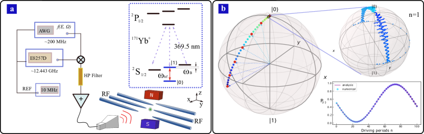
Figure 1: Experimental procedure to measure Floquet dynamics in a trapped-ion system. a) The qubit is encoded in the clock transition of a single trapped ${}^{171}\mathrm{Yb}^{+}$ion. The qubit is periodically driven by a microwave field generated by an AWG and a fixed-frequency signal source, which are both referenced to a 10 MHz rubidium frequency standard. b) On the right Bloch sphere, the qubit is initialized to $\left|0\right\rangle$ and evolves to $U(T)\left|0\right\rangle$ after one period of driving with function $f(E=16,\Omega=5)$. The fast dynamics (“micromotion”) of the qubit during this elementary period is shown on the Bloch sphere, and arises from the intrinsic time-dependence of the Floquet states $\left|\Phi_{j}(t)\right\rangle$. On the left Bloch sphere, the qubit starts from $\left|0\right\rangle$ (the north pole) and evolves to $U(nT)\left|0\right\rangle$ for multiple periods $n=1,2,3,...,30.$ The red dots are the points measured at $n=5,10,15,20,25,30$. The insert shows the probability $P_{\left|i\right\rangle}(n)$ when the qubit is measured onto base $\left|i\right\rangle=\frac{1}{\sqrt{2}}(\left|0\right\rangle+i\left|1\right\rangle)$ after n periods. $P_{\left|i\right\rangle}(n)$ is a sinusoidal function of $n$, with frequency proportional to the quasienergy $\epsilon_{j}(E)$. For values of $E$ satisfying $\epsilon_{j}(E)=0$, the state is frozen at $\left|0\right\rangle$ and $P_{\left|i\right\rangle}(n)=1/2$ for all $n$. Since $\epsilon_{j}(E)$ is proportional to the real part of $-\zeta(1/2+iE)/(1/2+iE)$, we can therefore identify Riemann zeros by observing the freezing of the dynamics, i.e. $P_{\left|i\right\rangle}=1/2$.

I.2 Experiment

The experimental results were obtained by periodically driving a single trapped ion with microwave fields. The two-level system is encoded in the hyper-fine clock transition $\left|0\right\rangle\equiv{}^{2}S_{1/2}\left|F=0,\thinspace m_{F}=0\right\rangle$ and $\left|1\right\rangle\equiv{}^{2}S_{1/2}\left|F=1,\thinspace m_{F}=0\right\rangle$ in a single ytterbium (${}^{171}\mathrm{Yb}^{+}$) ion confined in a Paul ion trap cui2016experimental , as shown in Fig. 1a. This clock qubit has the advantages of high-fidelity quantum operations and long coherence time OM07 ; WK17 . The tunneling, $J$, in this system is of the order of $10$kHz, giving a resonant Rabi time of $\sim 100\mu$s. The driving function is switched on by fast modulating the detuning frequency.

After 1 ms of Doppler cooling and 50 $\mu$s of optical pumping, the ion is initialized in the ground state $\left|0\right\rangle$ with a probability $\geq 99.5\%$. The qubit is then driven by a microwave field for multiple periods. The driving function was generated from a programmable arbitrary waveform generator (AWG) by phase modulating a 200 MHz microwave sinusoidal signal with the driving function $f(t)$. It is then mixed with a 12.4 GHz fixed frequency signal. The amplified microwave fields were delivered to the trapped ion from an horn antenna located outside the vacuum chamber. At the end of the multiple periods, the state is measured in the basis $\left|i\right\rangle=\frac{1}{\sqrt{2}}(\left|0\right\rangle+i\left|1\right\rangle)$ by applying a $\pi/4$ rotation and normal fluorescence detection. When more than one photon is detected, the measurement result is noted as 1; otherwise it is noted as 0. The time evolution of the state population is recorded as a function of the number of periods.

In Fig. 1b we show the experimental protocol, plotted on the Bloch sphere. As noted previously, the Floquet modes $\left|\Phi_{1}(E,\Omega,t)\right\rangle=a(t)\left|0\right\rangle+b(t)\left|1\right\rangle,\left|\Phi_{2}(E,\Omega,t)\right\rangle=b^{*}(t)\left|0\right\rangle-a^{*}(t)\left|1\right\rangle$ are the eigenstates of the one-period time evolution operator $U(E,\Omega)$, where $\Omega$ is the driving frequency, and $E$ is a driving parameter related to the argument of the zeta function, $\zeta(1/2+iE)$. Starting from the initial state $\left|0\right\rangle$, the population of the state measured in basis state $\left|i\right\rangle$ after $n$ periods of driving is $P(n,E,\Omega)=1/2-A\sin(2nT\epsilon_{j}(E,\Omega))$, where $A=\mathrm{Re}\{a(0)b^{*}(0)\}$, and $\epsilon_{j}(E,\Omega)$ is the quasienergy. It is clear that if $E$ is equal to the zeros of $\epsilon_{j}(E,\Omega)$, $\epsilon_{j}(E,\Omega)$ vanishes and $P(n,E,\Omega)=1/2$ for all $n$. While if $\epsilon_{j}(E,\Omega)\neq 0$, $P(n,\Omega,E)$ evolves sinusoidally with a frequency proportional to the quasienergy $\epsilon_{j}(E,\Omega)$. The the Riemann zeros can thus be identified by observing the freezing of the evolution of $P(n,E,\Omega)$ produced by CDT.

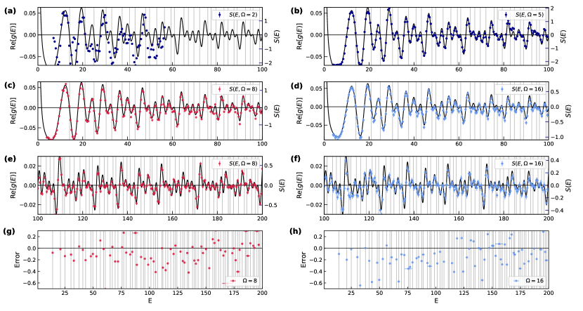
Figure 2: Identifying Riemann zeros by observing the frozen dynamics of the state. In (a-f), the black curve is the real part of $g(E)$. The vertical grey lines indicate the Riemann zeros, {14.1347, 21.022, 25.0109, 30.4249, 32.9351, …}; the other points where $g(E)$ crosses the axis correspond to the real part of the zeta function vanishing but not the imaginary part, and so do not represent Riemann zeros. The dots are the $S$ parameter which is defined as $S(\Omega,E)=\sum_{n}[P_{\left|i\right\rangle}(n,\Omega,E)-1/2]$, where $n=\{5,10,15,20,25,30\}$. $S(\Omega,E)$ is used to identify the Riemann zeros by observing $S=0$. (a) When $\Omega=2$, the high-frequency limit is not well satisfied, so the behaviour of $S(\Omega,E)$ does not match $g(E)$. (b) By contrast, $\Omega=5$ does give good agreement for $E\leq 100$. (c) Increasing $\Omega$ further to 8 provides even better agreement with $g(E)$. (e) We implemented the measurement for $E$ up to 200 and identified the first 80 Riemann zeros with high accuracy. (d, f) Results of $\Omega=16$. The measurement can be extended to higher $E$ without loss of efficiency and accuracy. Data points with $E\leq 100$ ($E\geq 100$) were obtained by 2000 (5000) measurements. The error bar $\delta S$ of $S(\Omega,E)$ is the sum of the statistical errors of the corresponding $P_{\left|i\right\rangle}(n,\Omega,E)$, where $n=\{5,10,15,20,25,30\}$, within one standard deviation. (g, h) Zeros were extracted by interpolating $S(E,\Omega)$ using a cubic polynomial 4000 times. Each time, $S$ is sampled randomly in [$S-\delta S$, $S+\delta S$]. The extracted zeros are the mean values of the interpolated zeros (see Supplementary Material). There are a few vertical lines with no red points on them. This means that the error is so large that the points don’t fall inside the plot range. The error (dot) is the difference between the extracted zeros and the exact zeros, with the error bars indicating the standard deviations of the mean values in the interpolation.

To give a quantitative characterization of the state evolution, we define the $S$ parameter as $S(\Omega,E)=\sum_{n}[P_{\left|i\right\rangle}(n,\Omega,E)-1/2]$, where $n=\{5,10,15,20,25,30\}$ are the number of driving periods in the experiment. It is straightforward to see that the zeros of the quasienergies are the zeros of $S(\Omega,E)$ as well. Therefore a scan of the parameter $E$ allows us to identify the Riemann zeros by observing $S(\Omega,E)=0$. To give a direct comparison, we show in Fig. 2 the experimental results of $S(\Omega,E)$ and the real part of $g(E)$ as a function of $E$ for $\Omega=2$, 5, 8, and 16, respectively. For $\Omega=2$, we can see that $S(\Omega,E)$ shows a significant distortion from the theoretical zeta function and does not allow the position of the Riemann zeros to be determined. Increasing $\Omega$, however, substantially improves the results, and gives excellent agreement between data and theory over the range $E\leq 200$, allowing the first eighty Riemann zeros to be resolved. This improvement occurs because larger values of $\Omega$ satisfy the high-frequency approximation better, and thus Eq. 1 becomes more precise. The difference between the measured zeros and the exact Riemann zeros is shown in Fig. 2 (g). Most of the zeros can be identified with an accuracy of 1 % or better. In Table 1 we present the agreement quantitatively for four different driving frequencies over a wide range of $E$. We give further, and more detailed, comparisons of the agreement in the Supplementary Material.

	$E_{1}$	$E_{10}$	$E_{30}$	$E_{50}$	$E_{70}$
Exact	14.135	49.774	101.318	143.112	182.207
$\Omega=5$	14.07(1)	49.26(19)
$\Omega=8$	14.06(2)	49.67(3)	101.13(3)	142.90(9)	182.28(6)
$\Omega=12$	13.99(4)	49.36(23)	101.31(3)	142.72(22)	182.14(6)
$\Omega=16$	14.03(3)	49.23(22)	101.33(5)	142.91(13)	181.98(8)

Table 1: Comparison of the experimentally measured Riemann zeros with the true values for different driving frequencies. Zeros were extracted by interpolating $S(E,\Omega)\pm\delta S$ with a cubic polynomial 4000 times, where $\delta S$ is the $1-\sigma$ standard deviation of $S$. Each time, $S$ is sampled randomly in [$S-\delta S$, $S+\delta S$]. The zeros are the mean of the interpolated zeros. The values in parentheses denote the standard deviation of the means in terms of the least significant digit.

Since increasing $\Omega$ further would satisfy the high-frequency limit better, it might be thought that the accuracy of the results can be improved by increasing the driving frequency to arbitrarily high values. This is not the case however. As we show in Methods, the best results will be obtained when the driving period $T$ is small enough to satisfy the high-frequency limit, while at the same time $T$ is sufficiently large for it to replace the upper limit of integration in Eq. 5. As a consequence of these opposing requirements, the best results will actually be obtained for mid-range frequencies. In Fig. 2 (d, f and h) we show the results for $\Omega=16$. Comparing with the $\Omega=8$ result reveals that increasing the frequency has not improved the accuracy of the results.

I.3 Reconstruction of prime numbers

In 1859 Riemann found a formula that gives the number of primes $\pi(x)$ below or equal to $x$ in terms of the non trivial zeros $\rho_{n}=\frac{1}{2}+iE_{n}$ riemann . A consequence of this result is that the function conrey

$$h(x)=-\sum_{\rho}x^{\rho}$$ (2)

has peaks at the primes $p$ and their powers $p^{n}$. Fig. 3 shows a truncation of (2) together with the function

$$J(x)=\sum_{n\geq 1}\frac{1}{n}\pi(x^{1/n})$$ (3)

that jumps by 1 at every prime and by $\frac{1}{n}$ at the power $p^{n}$. Notice that the experimental error in the zeros does not affect appreciably the location of the peaks.

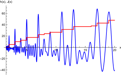
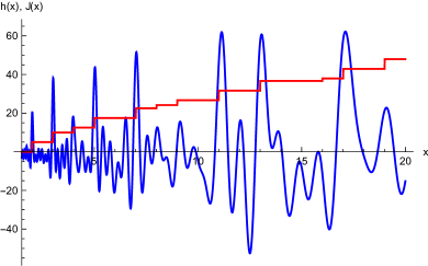
Figure 3: Primes from zeros. Plot of the function Eq. (2) with the sum restricted to $|E_{n}|<100$ (blue) and the function $5J(x)$ given in Eq. (3) (red). (a) using the exact values of $E_{n}$. (b) using the values of $E_{n}$ given in Table II (Extended Data) for $\Omega=16$. In both cases one can identify the first eight primes and their powers.

I.4 Conclusions

We have presented an experimental method for measuring the location of the zeros of the Riemann $\zeta$-function, by using Floquet engineering to control the quasienergy levels of a periodically-driven trapped ion. The experimentally measured values of the zeros are in excellent agreement with their theoretical values, and we have demonstrated how they can be used to reconstruct the prime numbers. The high level of experimental control over this system, and the implementation of a driving function derived from the complex function $g(E)=-\zeta(z)/z$ (where $z=1/2+iE$), allows as many as the first 80 zeros to be resolved. Our analysis indicates that there is a “sweet spot” for the driving frequency, in which $\Omega$ is sufficiently large for the system to be in the high-frequency regime, while its period is large in comparison to the width of the Fourier transform of $g(z)$. Using the experimentally measured zeros we have also obtained a good approximation of the lowest prime numbers. This reconstruction suggests the possibility of a direct experimental realization of the primes. The successful realization of the Riemann zeros in a quantum mechanical system represents an important step along a route inspired by the Hilbert and Pólya proposal, and may lead to further insights into the Riemann hypothesis.

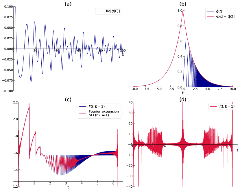
Figure 4: Derivation of the driving function. (a) The real component of $g(E)=-\zeta(1/2+iE)/(1/2+iE)$. (b) Van der Pol’s function is the Fourier transform, ${\tilde{g}}(t)$, of $g(E)$. The function is bounded by the red curve $\mathrm{exp}\left[-|t|/2\right]$, and contains an infinite number of finite discontinuities for positive $t$, arising from the floor function (see Eq. 4). (c) The primitive of the driving function, $F(t)$, for driving parameter $E=1$. The discontinuities in ${\tilde{g}}(t)$ give rise to discontinuities in this function as well. The red curve shows the Fourier expansion of $F(t)$, truncated at 500 terms. We can note how the fine detail is progressively blurred out as $t$ increases. (d) The driving function, $f(t)$, for $E=1$, obtained as $f(t)=\partial_{t}F(t)$, plotted over $0\leq t<T$. The discontinuities in $F(t)$ produce $\delta$-function spikes in the driving function. By construction, $f(t)$ is an even function of $t$, and so the full periodicity of this function is $2T$.

II Methods

II.1 Driving function derivation

Our starting point is the function $g(E)=\frac{-\zeta\left(\mbox{$\nicefrac{{1}}{{2}}$}+iE\right)}{\mbox{$\nicefrac{{1}}{{2}}$}+iE}$, where $\zeta(s)$ is the standard Riemann zeta function. We plot the behaviour of this function in Fig. 4a. As van der Pol showed in 1947, its Fourier transform (Fig. 4b) can be written in the surprisingly simple form vdp

$${\tilde{g}}(t)=e^{t/2}-e^{-t/2}[e^{t}]\ .$$ (4)

where $[x]$ is the integer part of $x$. As we can see from Fig. 4b, this function is localized around the origin, with an envelope of the form $\mathrm{exp}\left(-|t|/2\right)$.

By dividing the range of integration for the Fourier transform into two halves, it is straightforward to show that the real component of $g(E)$ is given by

$$\mathrm{Re}\left[g(E)\right]=\frac{2}{4E^{2}+1}+\int_{0}^{\infty}{\tilde{g}}(t)\cos Et\ dt\ .$$ (5)

In order to observe the location of the Riemann zeros, our interest is focused on values of $E>10$. Accordingly we can simply discard the first term, as over this range its magnitude is smaller than the experimental uncertainly in the measurements.

Our aim is to obtain a driving function $f(t)$ such that the effective tunneling is proportional to the real component of $g(E)$, that is, $\mathrm{Re}\left[J_{\mathrm{eff}}\right]=\alpha\ \mathrm{Re}\left[g(E)\right]$, where $\alpha$ is the constant of proportionality. Comparing Eq.(5) with Eq.(1), and assuming that the driving period $T$ is sufficiently large to replace the upper limit of integration in (5), reveals that $F(t)=\cos^{-1}\left(\alpha T{\tilde{g}}(t)\cos Et\right)$. The boundary condition $F(0)=0$ requires setting $\alpha=1/T$, which yields the final driving function $f(t)=\partial_{t}\left[\cos^{-1}\left({\tilde{g}}(t)\cos Et\right)\right]$. This choice of $\alpha$ also imposes the condition that the argument of the inverse cosine function is bounded within $\pm 1$ as required, since ${\tilde{g}}(0)$ is the global maximum of ${\tilde{g}}(t)$. We can note that replacing the upper limit of integration with $T$ represents an important restriction on the value of $\Omega$. This replacement means that $T$ must be large in comparison with the width of ${\tilde{g}}(t)$, and thus the driving frequency $\Omega$ must correspondingly be low. However, for Eq.(1) to be an accurate description of the system’s dynamics requires a high value of $\Omega$, so that the system is in the high-frequency regime. Therefore, good results will be obtained in an intermediate range of frequency, when both of these conditions can be adequately satisfied.

We show the form of the $F(t)$ and the driving function for a particular value of $E$ in Fig. 4c and Fig. 4d. The finite discontinuities present in $g(E)$ also produce discontinuities in $F(t)$, and thus $\delta$-function spikes in $f(t)$. A convenient way to obtain $f(t)$ numerically is to expand $F(t)$ in a Fourier series, differentiate the series term by term, and then to re-sum it. As in Ref.pra_1 , we want the driving function to be of definite parity, so that the two Floquet states will be of opposite parity, and so can cross as the driving parameter $E$ is varied. If this parity condition were not satisfied, the von Neumann-Wigner theorem would prevent the quasienergies becoming degenerate, and they could only form broader avoided crossings instead. For this reason we choose to expand $F(t)$ as a Fourier sine series, so that its derivative, $f(t)$ is a cosine series, and is thus an even function of time. Sufficient terms must be included in the series to ensure that the fine structure in $f(t)$ is reproduced with sufficient resolution. Typically in the experiment the series was truncated at 500 terms.

II.2 Experimental details

A long coherence time of the system is vital in the experiment. The hyperfine splitting of the (${}^{171}\mathrm{Yb}^{+}$) ion, $\omega_{hf}=\left(12642812118.5+\omega_{B}\right)$ Hz, has a second-order Zeeman shift $\omega_{B}=310.8B^{2}$, where $B$ is the magnetic field. We used $\mathrm{Sm}_{2}\mathrm{Co}_{17}$ permanent magnets to generate a static magnetic field of around $B=9.15$ G to reduce the 50 Hz ac-line noise. The whole platform is shielded in a 2-mm-thick $\mu$-metal enclosure to reduce the residual fluctuating magnetic fields RP16 . During the experiment, we still observed a slow drift of $\sim\pm 30$ Hz of the clock transition in 10 hours. This corresponds to $\Delta B\sim\pm 0.005$ G, which is mainly due to the temperature drift in the laboratory. This drift is not negligible. Therefore the clock transition frequency was frequently measured by Ramsey type measurements and calibrated by updating the AWG wave frequency during the experiment every half hour.

III Data availability

Source data and all other data that support the plots within this paper and other findings of this study are available from the corresponding author upon reasonable request.

Acknowledgments CEC was supported by the Spanish MINECO through grant FIS2017-84368-P, and GS by PGC2018-095862-B-C21, QUITEMAD+ S2013/ICE-2801, SEV-2016-0597 and the CSIC Research Platform on Quantum Technologies PTI-001. RH, MZA, JMC, YFH, YJH, CFL, and GCG were supported by the National Key Research and Development Program of China (Grants No.2017YFA0304100 and No. 2016YFA0302700), the National Natural Science Foundation of China (Grants No.11874343, No. 61327901, No. 11774335, and No. 11734015), Key Research Program of Frontier Sciences, CAS (Grant No. QYZDY-SSW-SLH003), the Fundamental Research Funds for the Central Universities (Grants No. WK2470000026, No. WK2470000027, and No. WK2470000028), and Anhui Initiative in Quantum Information Technologies (Grants No. AHY020100 and No. AHY070000).

Author Information CEC and GS developed the theoretical proposal. RH, MZA, JMC and YFH designed and performed the experiment. YJH, CFL and GCG supervised the experiments. All authors contributed to the data analysis, progression of the project, discussion of the results and the writing of the manuscript.

Extended Data

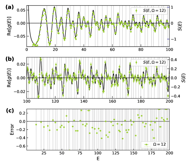
Figure 5: Identifying Riemann zeros by observing the frozen dynamics of the state for $\Omega=12$. In (a, b), the black curve is the real part of $g(E)$. The vertical grey lines indicate the Riemann zeros, e.g., {14.1347, 21.022, 25.0109, 30.4249, 32.9351, …}. The other points where $g(E)$ crosses the zero axis correspond to the real part of the zeta function vanishing but not the imaginary part, and so do not represent Riemann zeros. The dots are the $S$ parameter which is defined as $S(\Omega,E)=\sum_{n}[P_{\left|i\right\rangle}(n,\Omega,E)-1/2]$, where $n=\{5,10,15,20,25,30\}$. $S(\Omega,E)$ is used to identify the Riemann zeros by observing $S=0$. $S(\Omega=12,E)$ shows an excellent consistency in behavior with $g(E)$ for both (a) $0\leq E\leq 100$ and (b) $100\leq E\leq 200)$ and thus acts as a good indicator of the location of the Riemann zeros . The first 80 Riemann zeros can be identified with high accuracy. The measurement can be extended to higher $E$ without loss of efficiency and accuracy. Data points with $E\leq 100$ ($E\geq 100$) were obtained by 2000 (5000) measurements. The error bar $\delta S$ of $S(\Omega,E)$ is the sum of the statistical errors of the corresponding $P_{\left|i\right\rangle}(n,\Omega,E)$, where $n=\{5,10,15,20,25,30\}$, within one standard deviation. (c) Zeros were extracted by interpolating $S(E,\Omega)$ using a cubic polynomial 4000 times. Each time, $S$ is sampled randomly in [$S-\delta S$, $S+\delta S$]. The extracted zeros are the mean values of the interpolated zeros (see Table S1 and Table S2). The error (dot) is the difference between the extracted zeros and the exact zeros, with the error bars indicating the standard deviations of the mean values in the interpolation.

No.	Exact	$\Omega=5$	$\Omega=8$	$\Omega=12$	$\Omega=16$
1	14.135	14.07(1)	14.06(2)	13.99(4)	14.03(3)
2	21.022	21.04(2)	21.00(2)	20.93(5)	20.82(3)
3	25.011	24.70(3)	24.87(2)	24.87(7)	24.99(4)
4	30.425	30.59(2)	30.31(2)	30.29(3)	30.27(4)
5	32.935	32.76(3)	32.72(3)	32.57(8)	32.29(23)
6	37.586	37.64(2)	37.62(2)	37.39(2)	37.59(4)
7	40.919	40.95(2)	40.89(3)	40.78(3)	40.70(4)
8	43.327	42.85(9)	43.12(4)	43.23(4)	42.74(40)
9	48.005	48.23(4)	47.87(6)	47.94(6)	47.75(9)
10	49.774	49.26(19)	49.67(3)	49.36(23)	49.23(22)
11	52.970	52.93(2)	52.83(4)	52.88(5)	52.78(5)
12	56.446	56.56(3)	56.58(3)	56.28(3)	56.49(5)
13	59.347	59.44(5)	59.33(9)	59.35(6)	59.08(28)
14	60.832	60.10(48)	60.13(414)	60.41(144)	60.67(9)
15	65.113	65.53(11)	64.99(4)	65.05(6)	64.92(6)
16	67.080	67.06(5)	67.10(3)	66.98(10)	66.50(40)
17	69.546	69.36(4)	69.32(7)	69.11(28)	69.44(7)
18	72.067	71.82(3)	71.84(3)	71.76(8)	71.95(7)
19	75.705	76.33(37)	75.72(12)	75.23(332)	75.35(317)
20	77.145	76.84(8)	77.41(6)	76.80(9)	76.82(83)
21	79.337	78.89(6)	79.26(2)	78.95(4)	79.09(9)
22	82.914	84.12(117)	82.80(2)	82.67(4)	82.74(8)
23	84.736	84.82(2)	84.67(3)	84.31(12)	84.58(8)
24	87.425	87.50(7)	87.69(244)	87.23(6)	87.20(8)
25	88.809	87.93(47)	88.52(3)	88.33(47)	88.70(128)
26	92.492	92.96(4)	92.34(3)	92.37(5)	92.24(6)
27	94.651	94.55(59)	94.97(12)	94.34(144)	94.34(211)
28	95.871	95.82(8)	95.69(5)	94.66(290)	95.13(125)
29	98.831	98.87(3)	98.55(6)	98.69(4)	98.74(6)

Table 2: Comparison of the experimentally measured Riemann zeros with the true values ($1\leq E\leq 100$) for different driving frequencies. Zeros were extracted by interpolating $S(E,\Omega)\pm\delta S$ with a cubic polynomial 4000 times, where $\delta S$ is the $1-\sigma$ standard deviation of $S$. Each time, $S$ is sampled randomly in [$S-\delta S$, $S+\delta S$]. The zeros are the mean of the interpolated zeros. The values in parentheses denote the standard deviation of the means in terms of the least significant digit.

No.	Exact	$\Omega=8$	$\Omega=12$	$\Omega=16$
30	101.318	101.13(3)	101.31(3)	101.33(5)
31	103.726	103.50(4)	103.74(9)	103.66(5)
32	105.447	105.03(16)	105.49(7)	104.46(58)
33	107.169	106.03(112)	106.99(17)	106.93(5)
34	111.030	111.03(16)	111.60(227)	110.27(173)
35	111.875	111.54(19)	111.88(7)	112.86(337)
36	114.320	113.94(10)	114.49(9)	114.06(6)
37	116.227	115.96(11)	116.12(6)	115.82(20)
38	118.791	118.77(3)	118.71(4)	118.96(7)
39	121.370	121.27(6)	121.78(97)	122.26(69)
40	122.947	122.99(22)	123.48(323)	123.12(5)
41	124.257	122.82(48)	124.43(19)	123.85(38)
42	127.517	127.46(3)	127.51(4)	127.36(7)
43	129.579	129.36(32)	129.66(12)	129.57(12)
44	131.088	130.84(16)	130.91(156)	131.22(5)
45	133.498	133.41(7)	134.00(36)	133.62(12)
46	134.757	134.34(24)	134.89(132)	134.45(27)
47	138.116	138.14(8)	138.27(10)	138.12(11)
48	139.736	139.52(6)	139.98(9)	139.72(9)
49	141.124	140.86(8)	141.20(5)	140.57(107)
50	143.112	142.90(9)	142.72(22)	142.91(13)
51	146.001	146.03(8)	145.80(4)	146.24(52)
52	147.423	147.34(8)	147.17(46)	147.43(11)
53	150.054	150.04(6)	149.62(73)	150.10(125)
54	150.925	150.20(414)	149.47(197)	150.96(22)
55	153.025	152.68(6)	152.79(5)	152.89(14)
56	156.113	156.27(10)	156.02(203)	156.19(343)
57	157.598	157.69(20)	157.60(89)	157.40(15)
58	158.850	159.16(379)	158.84(89)	158.57(79)
59	161.189	161.32(8)	161.00(4)	161.25(3)
60	163.031	163.00(5)	162.43(58)	162.75(12)
61	165.537	165.41(5)	165.94(26)	165.71(14)
62	167.184	167.13(5)	167.08(11)	167.42(85)
63	169.095	168.49(458)	169.16(49)	169.01(14)
64	169.912	169.18(67)	169.17(27)	169.80(138)
65	173.412	173.33(5)	173.60(19)	173.36(8)
66	174.754	174.75(3)	174.65(7)	174.40(105)
67	176.441	176.23(11)	176.52(16)	176.41(13)
68	178.377	177.97(175)	178.26(10)	178.11(11)
69	179.916	179.89(5)	180.01(262)	179.36(51)
70	182.207	182.28(6)	182.14(6)	181.98(8)
71	184.874	185.51(294)	184.82(17)	184.77(86)
72	185.599	185.89(223)	185.43(24)	184.60(328)
73	187.229	187.10(188)	187.04(72)	187.22(34)
74	189.416	189.50(0)	189.28(6)	189.23(6)
75	192.027	192.07(9)	192.20(169)	192.42(41)
76	193.080	193.09(4)	193.10(12)	193.06(159)
77	195.265	195.56(217)	195.18(80)	195.55(58)
78	196.876	196.93(28)	196.04(304)	196.81(9)
79	198.015	196.81(42)	197.74(10)	197.80(154)
80	201.265	199.24(576)	200.14(5)	200.47(16)

Table 3: Comparison of the experimentally measured Riemann zeros with the true values ($100\leq E\leq 200$) for different driving frequencies. Zeros were extracted by interpolating $S(E,\Omega)\pm\delta S$ with a cubic polynomial 4000 times, where $\delta S$ is the $1-\sigma$ standard deviation of $S$. Each time, $S$ is sampled randomly in [$S-\delta S$, $S+\delta S$]. The zeros are the mean of the interpolated zeros. The values in parentheses denote the standard deviation of the means in terms of the least significant digit.

References

- (1)
- (2) H.M. Edwards, Riemann’s Zeta Function (New York: Academic), 1974.
- (3) B. Riemann, “On the Number of Prime Numbers less than a Given Quantity”, Monatsberichte der Berliner Akademie November 1859, 671 (1859), English version.
- (4) https://www.claymath.org/millennium-problems.
- (5) J.B. Conrey, ”The Riemann Hypothesis”, Not. Am. Math. Soc. 50, (2003).
- (6) M. V. Berry, “Hearing the music of the primes: auditory complementarity and the siren song of zeta”, J. Phys. A: Math.Theor. 45, 382001 (2012).
- (7) H. L. Montgomery “The pair correlation of the zeta function”, in: Proc. Sympos. Pure Math. vol. XXIV, St. Lois. Mo. 1972. Amer. Math. Soc., Providence, R.I. (1973).
- (8) H. L. Montgomery, “Distribution of the zeros of the Riemann zeta function”, in Proceedings Int. Cong. Math. Vancouver 1974, Vol. I, Canad. Math. Congress, Montreal, 379 (1975).
- (9) A.M. Odlyzko, “On the distribution of spacings between zeros of the zeta function”, Math. Comp. 48, 273 (1987).
- (10) M. V. Berry, “Riemann’s zeta function: a model for quantum chaos?”, in Quantum Chaos and Statistical Nuclear Physics, edited by T. H. Seligman and H. Nishioka, Springer Lecture Notes in Physics Vol. 263 , p. 1, Springer, New York (1986).
- (11) M.V. Berry, “Semiclassical formula for the number variance of the Riemann zeros”, Nonlinearity 1 (1988), 399-407.
- (12) E. B. Bogomolny and J. P. Keating, “Gutzwiller’s trace formula and spectral statistics: beyond the diagonal approximation”, Phys. Rev. Lett. 77 (1996), 1472-1475.
- (13) M. V. Berry and J. P. Keating, “The Riemann zeros and eigenvalue asymptotics”, SIAM Rev. 41 (1999), 236-266.
- (14) A. Connes, “Trace formula in noncommutative geometry and the zeros of the Riemann zeta function”, Selecta Mathematica New Series 5 29, (1999).
- (15) G. Sierra and J. Rodriguez-Laguna, “The H = xp model revisited and the Riemann zeros”, Phys. Rev. Lett. 106, 200201 (2011).
- (16) M. V. Berry and J. P. Keating, “A compact hamiltonian with the same asymptotic mean spectral density as the Riemann zeros”, J. Phys. A: Math. Theor. 44, 285203 (2011).
- (17) M. Srednicki, “The Berry-Keating Hamiltonian and the Local Riemann Hypothesis”, J. Phys. A: Math. Theor. 44, 305202 (2011).
- (18) C.M. Bender, D.C. Brody, M.P. Müller, “Hamiltonian for the zeros of the Riemann zeta function”, Phys. Rev.Lett. 118, 130201 (2017).
- (19) G. Sierra, “The Riemann zeros as spectrum and the Riemann hypothesis”, Symmetry 2019, 11(4), 494.
- (20) C.E. Creffield, “Location of crossings in the Floquet spectrum of a driven two-level system”, Phys. Rev. B 67, 165301 (2003).
- (21) F. Grossmann, T. Dittrich, P. Jung, and P. Hänggi, “Coherent destruction of tunneling”, Phys. Rev. Lett. 67, 516 (1991).
- (22) B. van der Pol, “An electro-mechanical investigation of the Riemann zeta function in the critical strip”, Bull. Am. Math. Soc. 53 976–81 (1947).
- (23) M.V. Berry, “Riemann zeros in radiation patterns”, J. Phys. A: Math. Theor. 45, 302001 (2012).
- (24) C.E. Creffield and G. Sierra Phys. Rev. A 91, 063608 (2015).
- (25) R. He, et al. “Identifying the Riemann zeros by periodically driving a single qubit”, Phys. Rev. A 101, 043402 (2020).
- (26) L.M. Cui, et al. “Experimental Trapped-ion Quantum Simulation of the Kibble-Zurek dynamics in momentum space”, Sci. Rep. 6, 33381 (2016).
- (27) S. Olmschenk, et al. “Manipulation and detection of a trapped Yb+ hyperfine qubit”. Phys. Rev. A 76, 5, 052314 (2007).
- (28) Y. Wang, et al. “Single-qubit quantum memory exceeding ten-minute coherence time”. Nat. Photon 11, 646–650 (2017).
- (29) T. Ruster, et al. ”A long-lived Zeeman trapped-ion qubit”, Appl. Phys. B 122, 10, 254 (2016).