Strong Brascamp–Lieb Inequalities

Abstract

In this paper, we derive sharp nonlinear dimension-free Brascamp–Lieb inequalities (including hypercontractivity inequalities) for distributions on Polish spaces, which strengthen the classic Brascamp–Lieb inequalities. Applications include the extension of Mrs. Gerber’s lemma to the cases of Rényi divergences and distributions on Polish spaces, the strengthening of small-set expansion theorems, and the characterization of the exponent of the $q$-stability. Our proofs in this paper are based on information-theoretic and coupling techniques.

1 Introduction

Let $\mathcal{X}$ and $\mathcal{Y}$ be two Polish spaces, and $\mathbb{B}_{\mathcal{X}}$ and $\mathbb{B}_{\mathcal{Y}}$ the Borel $\sigma$-algebras on $\mathcal{X}$ and $\mathcal{Y}$ respectively. Let $(\mathcal{X}\times\mathcal{Y},\mathbb{B}_{\mathcal{X}}\otimes\mathbb{B}_{\mathcal{Y}})$ be the product of the measurable spaces $(\mathcal{X},\mathbb{B}_{\mathcal{X}})$ and $(\mathcal{Y},\mathbb{B}_{\mathcal{Y}})$, and $P_{XY}$ a probability measure (also termed distribution) on $(\mathcal{X}\times\mathcal{Y},\mathbb{B}_{\mathcal{X}}\otimes\mathbb{B}_{\mathcal{Y}})$. The (forward and reverse) Brascamp–Lieb (BL) inequalities are as follows: Given the distribution $P_{XY}$ and $p,q\in\overline{\mathbb{R}}:=[-\infty,\infty]$, for any nonnegative measurable functions $f:\mathcal{X}\to[0,\infty),g:\mathcal{Y}\to[0,\infty),$

$$\langle f,g\rangle \leq e^{-\underline{C}}\|f\|_{p}\|g\|_{q}$$ (1.1)

$$\langle f,g\rangle \geq e^{-\overline{C}}\|f\|_{p}\|g\|_{q},$$ (1.2)

where $\langle f,g\rangle:=\int fg\mathrm{d}P_{XY},$

$$\|f\|_{p}:=\begin{cases}(\int f^{p}\mathrm{d}P_{X})^{1/p}&p\notin\{0,\pm\infty\}\\ e^{\mathbb{E}[\log f]}&p=0\textrm{ and }\mathbb{E}[\log f]\textrm{ exists}\\ \infty&p=0\textrm{ and }\mathbb{E}[\log f]\textrm{ does not exist}\\ \lim_{p\to\infty}\|f\|_{p}&p=\infty\\ \lim_{p\to-\infty}\|f\|_{p}&p=-\infty\end{cases}$$

and $\|g\|_{q}$ is defined similarly but with $(f,P_{X},p)$ replaced by $(g,P_{Y},q)$, and $\underline{C}=\underline{C}_{p,q}$ and $\overline{C}=\overline{C}_{p,q}$ only depend on $p,q$ given the distribution $P_{XY}$. We denote the optimal exponents $\underline{C}_{p,q}$ and $\overline{C}_{p,q}$ for the distribution $P_{XY}$ as $\underline{C}_{p,q}^{*}$ and $\overline{C}_{p,q}^{*}$. Throughout this paper, we exclude the trivial case that $P_{X}$ or $P_{Y}$ is a Dirac measure.

Note that the BL inequalities are homogeneous, i.e., (1.1) and (1.2) still hold if we scale the functions $f,g$ respectively by two positive real values $a,b$. Hence, without changing the optimal exponents, we can normalize both sides of the BL inequalities in (1.1) and (1.2) by $\|f\|_{\hat{p}}\|g\|_{\hat{q}}$ for reals $\hat{p}\neq p,\hat{q}\neq q$. The resulting normalized version of BL inequalities can be understood as a linear tradeoff between the correlation $\frac{\langle f,g\rangle}{\|f\|_{\hat{p}}\|g\|_{\hat{q}}}$ and the product $\frac{\|f\|_{p}}{\|f\|_{\hat{p}}}\frac{\|g\|_{q}}{\|g\|_{\hat{q}}}$. In this paper, we aim at studying the optimal nonlinear tradeoff among $\frac{\langle f,g\rangle}{\|f\|_{\hat{p}}\|g\|_{\hat{q}}},\frac{\|f\|_{p}}{\|f\|_{\hat{p}}}$, and $\frac{\|g\|_{q}}{\|g\|_{\hat{q}}}$. To this end, we first need introduce the $L_{p}$-norm and a new concept termed $(p,\hat{p})$-entropy.

1.1 Preliminaries on (Pseudo) $L_{p}$-Norms

Throughout this paper, when we write a function $f:\mathcal{X}\to[0,\infty)$, by default, we mean that it is measurable. A similar convention also applies to a function $g:\mathcal{Y}\to[0,\infty)$. Let $\Phi(\mathcal{Z}):=\{h:\mathcal{Z}\to[0,\infty)\}\backslash\{h=0\textrm{ a.s.}\}$ for $\mathcal{Z}=\mathcal{X}$ or $\mathcal{Y}$, which is the set of nonenegative measurable functions but excluding the zero function. Throughout this paper, we suppose that $f\in\Phi(\mathcal{X})$ and $g\in\Phi(\mathcal{Y})$. The $p$-norm (or $p$-pseudo norm) $\|\cdot\|_{p}$ satisfies the following properties.

Lemma 1.

The following hold.

1. Given $f\in\Phi(\mathcal{X})$, $\|f\|_{p}$ is nondecreasing in the order $p\in\overline{\mathbb{R}}$.

2. If $\mathbb{E}[\log f]$ exists, then, $\lim_{r\downarrow 0}\|f\|_{r}=\|f\|_{0}$ if $\|f\|_{s}<\infty$ for some $s>0$, and $\lim_{r\uparrow 0}\|f\|_{r}=\|f\|_{0}$ if $\|f\|_{s}>0$ for some $s<0$. Furthermore, if $\mathbb{E}[\log f]$ does not exist, then $\|f\|_{s}=\infty$ for all $s>0$, and $\|f\|_{s}=0$ for all $s<0$.

3. $\|f\|_{\infty}$ is equal to the essential supremum of $f$.

4. $\|f\|_{-\infty}$ is equal to the essential infimum of $f$.

5. If $P_{X}(f>0)<1$, i.e., $f$ is not positive a.e., then $\|f\|_{p}=0$ for $p\in[-\infty,0]$.

6. Given $f\in\Phi(\mathcal{X})$, $\|f\|_{p}$ is continuous in the order $p\in\{p\in\overline{\mathbb{R}}:\|f\|_{p}<\infty\}$.

7. For $p\in(0,\infty]$, $\|f\|_{p}=0$ if and only if $f=0$ a.e. Hence, for $f\in\Phi(\mathcal{X})$, we always have $\|f\|_{p}>0$ for $p\in(0,\infty]$.

8. For $p\in[-\infty,0)$, $\|f\|_{p}=\infty$ if and only if $f=\infty$ a.e. Hence, for any $f:\mathcal{X}\to[0,\infty)$, we always have $\|f\|_{p}<\infty$ for $p\in[-\infty,0)$.

Proof.

Statement 1 follows by Jensen’s inequality. Statement 2 follows by the following argument. For $t>0$, define $h(s)=\frac{t^{s}-1}{s}$ if $s\neq 0$, and $\log t$ otherwise. Then, $h$ is nondecreasing on the whole real line. This immediately implies that if $\|f\|_{s}<\infty$ for some $s>0$, then $\int_{\{f>1\}}\log f\mathrm{d}P_{X}$ is finite. Hence, the second part of Statement 2 holds. Furthermore, combined with the existence of $\mathbb{E}[\log f]$, it implies that $\mathbb{E}[|\log f|]$ is finite. Substituting $f\leftarrow f^{s}$ into the formula in [3, Exercise 2.12.91] yields the first part of Statement 2 for $s>0$. The part for $s<0$ follows similarly, in which case, substituting $f\leftarrow f^{s}$ with $s<0$ into the formula in [3, Exercise 2.12.91] yields the first part of Statement 2 for $s<0$. Statement 6 follows by the following argument. For $p=0$, it follows from Statement 2. We next consider the case $p\neq 0$. We partition $\mathcal{X}$ into two disjoint sets $\{f\geq 1\}$ and $\{f<1\}$, and decompose the integral in the definition of $\|f\|_{p}$ into two parts according to this partition. For $p>0$, we apply Lebesgue’s dominated convergence theorem to the integral on set $\{f<1\}$, and apply Beppo Levi’s lemma on the monotone convergence to the integral on set $\{f\geq 1\}$. Then, we have $\lim_{r\uparrow p}\|f\|_{r}=\|f\|_{p}$. Similarly, Statement 6 for other cases can be proven. ∎

Based on Statements 1, 7, and 8 above, to ensure that $0<\|f\|_{p}<\infty$ for $f\in\Phi(\mathcal{X})$ and $p\in\overline{\mathbb{R}}\backslash\{0\}$, it suffices to require $\|f\|_{p}>0$ if $p<0$, and $\|f\|_{p}<\infty$ if $p>0$. Hence, if we define

$$\mathcal{D}_{f}:=\{p\in\overline{\mathbb{R}}:0<\|f\|_{p}<\infty\},$$

then for $f\in\Phi(\mathcal{X})$, $\mathcal{D}_{f}$ corresponds to the union of $\{p\in[-\infty,0):\|f\|_{p}>0\}$, $\{p\in(0,\infty]:\|f\|_{p}<\infty\}$, and also $\{0\}$ if $0<\|f\|_{0}<\infty$. Note that $\mathcal{D}_{f}$ is an interval.

1.2 Two-Parameter Version of Entropies

Throughout this subsection, we assume $f\in\Phi(\mathcal{X})$. We call $p$ as a simple order if $p\in\mathbb{R}\backslash\{0\}$, and call $p$ as an extended order if $p\in\overline{\mathbb{R}}$. We first define the $(p,\hat{p})$-entropy for a pair of simple orders. For convenience, we denote

$$\mathcal{R}_{f}:=\mathcal{D}_{f}\cup\{0\}.$$

Here, the $0$-pseudo norm is excluded since it will not be used in the definition of $(p,\hat{p})$-entropy, and in fact, the $(p,0)$- or $(0,p)$-entropy will be defined by the continuous extension. Given $p,\hat{p}\in\mathcal{R}_{f}\backslash\{0,\pm\infty\}$ such that $p\neq\hat{p}$, we define the $(p,\hat{p})$-entropy of $f$ as

$$\operatorname{Ent}_{p,\hat{p}}(f):=\frac{p\hat{p}}{p-\hat{p}}\log\frac{\|f\|_{p}}{\|f\|_{\hat{p}}}.$$ (1.3)

For $p,\hat{p}$ with $p\neq\hat{p}$, one of them being in $\mathbb{R}\backslash\{0\}$, and the other being in $\mathbb{R}\backslash\mathcal{R}_{f}$ (i.e., $\|f\|_{p}$ or $\|f\|_{\hat{p}}$ being zero or $\infty$), we define $\operatorname{Ent}_{p,\hat{p}}(f):=\infty$ if $p\hat{p}>0$, and $\operatorname{Ent}_{p,\hat{p}}(f):=-\infty$ if $p\hat{p}<0$.

The $(p,\hat{p})$-entropies for other cases are defined by continuous extensions. Specifically, for $p\in\mathcal{R}_{f}\backslash\{0,\pm\infty\}$, the $(p,p)$-entropy of $f$ is defined as

$$\operatorname{Ent}_{p,p}(f):=\lim_{\hat{p}/p\uparrow 1}\operatorname{Ent}_{p,\hat{p}}(f)=\operatorname{Ent}_{p}(f):=\frac{\mathbb{E}[f^{p}\log f^{p}]-\mathbb{E}[f^{p}]\log\mathbb{E}[f^{p}]}{\mathbb{E}[f^{p}]},$$ (1.4)

and for $p\in\mathbb{R}\backslash\mathcal{R}_{f}$,

$$\operatorname{Ent}_{p,p}(f):=\operatorname{Ent}_{p}(f):=\infty.$$ (1.5)

Note that the usual entropy of $f^{p}$ corresponds to the numerator in the right-hand side (RHS) of (1.4). Hence, $\operatorname{Ent}_{p}(f)$ coincides the normalized version of the entropy of $f^{p}$.

We next define the $(p,\hat{p})$-entropy for a pair of orders such that at least one of them is an extended order. For $p\in\mathcal{R}_{f}$, the $(p,0)$-entropy and the $(0,p)$-entropy of $f$ are defined by

$$\operatorname{Ent}_{p,0}(f),\;\operatorname{Ent}_{0,p}(f):=\operatorname{Ent}_{0}(f):=-\log P_{X}(f>0).$$

For $p\notin\mathcal{R}_{f}$, we

$$\operatorname{Ent}_{p,0}(f),\;\operatorname{Ent}_{0,p}(f):=\begin{cases}\infty&p\in(0,\infty]\\ -\infty&p\in[-\infty,0)\end{cases}.$$

For $p\in\overline{\mathbb{R}}\backslash\{0\}$, the $(p,\infty)$-entropy and the $(\infty,p)$-entropy of $f$ satisfying $\|f\|_{\infty}<\infty$ are defined by

$$\operatorname{Ent}_{p,\infty}(f),\;\operatorname{Ent}_{\infty,p}(f):=\begin{cases}\lim_{\hat{p}\uparrow\infty}\operatorname{Ent}_{p,\hat{p}}(f)=-p\log\frac{\|f\|_{p}}{\|f\|_{\infty}}&p\in\mathbb{R}\backslash\{0\}\\ \lim_{p\uparrow\infty}\operatorname{Ent}_{p,\infty}(f)=\operatorname{Ent}_{\infty}(f):=-\log P_{X}(f=\|f\|_{\infty})&p=\infty\\ \lim_{p\downarrow-\infty}\operatorname{Ent}_{p,\infty}(f)=0&f\textrm{ is constant},\;p=-\infty\\ \lim_{p\downarrow-\infty}\operatorname{Ent}_{p,\infty}(f)=-\infty&f\textrm{ is not constant},\;p=-\infty\end{cases}.$$

For $f$ satisfying $\|f\|_{\infty}=\infty$,

$$\operatorname{Ent}_{p,\infty}(f),\;\operatorname{Ent}_{\infty,p}(f):=\begin{cases}\infty&p\in(0,\infty]\\ -\infty&p\in[-\infty,0)\end{cases}.$$

For $p\in[-\infty,\infty)\backslash\{0\}$, the $(p,-\infty)$-entropy and the $(-\infty,p)$-entropy of $f$ satisfying $\|f\|_{-\infty}>0$ (which implies $f>0$ a.e.) are defined by

$$\operatorname{Ent}_{p,-\infty}(f),\;\operatorname{Ent}_{-\infty,p}(f):=\begin{cases}\lim_{\hat{p}\downarrow-\infty}\operatorname{Ent}_{p,\hat{p}}(f)=-p\log\frac{\|f\|_{p}}{\|f\|_{-\infty}}&p\in\mathbb{R}\backslash\{0\}\\ \lim_{p\downarrow-\infty}\operatorname{Ent}_{p,-\infty}(f)=\operatorname{Ent}_{-\infty}(f):=-\log P_{X}(f=\|f\|_{-\infty})&p=-\infty\end{cases}.$$

For $f$ satisfying $\|f\|_{-\infty}=0$,

$$\operatorname{Ent}_{p,-\infty}(f),\;\operatorname{Ent}_{-\infty,p}(f):=\begin{cases}-\infty&p\in(0,\infty)\\ \infty&p\in[-\infty,0)\end{cases}.$$

Lemma 2.

It holds that $\operatorname{Ent}_{p,\hat{p}}(f)=\operatorname{Ent}_{\hat{p},p}(f)=\operatorname{Ent}_{p/s,\hat{p}/s}(f^{s})=\operatorname{Ent}_{\hat{p}/s,p/s}(f^{s})$ for $s\neq 0$.

The $(p,\hat{p})$-entropy defined above is closely related to the well-known Rényi divergences in information theory. For $s\in\mathbb{R}\backslash\{0,1\}$, the Rényi divergence of order $s$ is defined as $D_{s}(Q\|P):=\frac{1}{s-1}\log\int(\frac{\mathrm{d}Q}{\mathrm{d}\mu})^{s}(\frac{\mathrm{d}P}{\mathrm{d}\mu})^{1-s}\mathrm{d}\mu$ for a nonnegative finite measure $\mu$ (in fact, the value of $D_{s}(Q\|P)$ is independent of the choice of $\mu$), where $\frac{\mathrm{d}P}{\mathrm{d}\mu}$ denotes the Radon–Nikodym derivative of $P$ w.r.t. $\mu$. For $s\in\{0,1,\pm\infty\}$, the Rényi divergence of order $s$ is defined by the continuous extension. For $s=1$, the Rényi divergence of order $1$, also termed the Kullback–Leibler divergence, or simply, the KL divergence, is $D(Q\|P):=\int\log(\frac{\mathrm{d}Q}{\mathrm{d}P})\mathrm{d}Q$ if $Q\ll P$, and otherwise, $D(Q\|P):=\infty$. Here and throughout this paper, we adopt the conventions that $\log 0=-\infty,\log\infty=\infty$ and $0\log 0=0$. The $(p,\hat{p})$-entropy and the Rényi divergence of order $\hat{p}/p$ admit the following intimate relationship.

Lemma 3.

For $f\in\Phi(\mathcal{X})$ and $p\in\mathcal{R}_{f}\backslash\{0,\pm\infty\}$, we can write $\frac{f^{p}}{\|f\|_{p}^{p}}$ as a Radon–Nikodym derivative $\frac{\mathrm{d}Q_{X}}{\mathrm{d}P_{X}}$. Then, for such $p$ and together with $\hat{p}\in\overline{\mathbb{R}}$,

$$\operatorname{Ent}_{p,\hat{p}}(f)=D_{\hat{p}/p}(Q_{X}\|P_{X}).$$ (1.6)

Throughout this paper, we use the convention $\infty\cdot 0=-\infty\cdot 0=0$.

Lemma 4.

For $f\in\Phi(\mathcal{X})$, the following hold.

1. $\operatorname{Ent}_{p,\hat{p}}(f)\geq 0$ for $p,\hat{p}\geq 0$ or $p,\hat{p}<0$.

2. $\operatorname{Ent}_{p,\hat{p}}(f)\leq 0$ for $p<0\leq\hat{p}$ or $\hat{p}<0\leq p$.

3. For $p\hat{p}\neq 0$, $\operatorname{Ent}_{p,\hat{p}}(f)=0$ if and only if $f$ is constant a.e.

4. For $p\hat{p}=0$, $\operatorname{Ent}_{p,\hat{p}}(f)=0$ if and only if $f$ is positive a.e. and $p,\hat{p}\in\mathcal{R}_{f}$.

5. $\operatorname{Ent}_{p,\hat{p}}(f)$ is nondecreasing in $\hat{p}\in\overline{\mathbb{R}}$ given $p\in[0,\infty]$, and nonincreasing in $\hat{p}\in\overline{\mathbb{R}}$ given $p\in[-\infty,0)$.

Proof.

Statements 1)-4) follow by definition or by the equivalence in (1.6).

We now prove Statement 5). For $p\in(0,\infty)\cap\mathcal{R}_{f}$, (1.6) holds. Hence, by the monotonicity of the Rényi divergence in its order [4], $\operatorname{Ent}_{p,\hat{p}}(f)$ is nondecreasing in $\hat{p}\in\mathcal{R}_{f}$ given $p\in(0,\infty)\cap\mathcal{R}_{f}$. The monotonicity for other $p$ can be verified similarly. In fact, the monotonicity of $\hat{p}\mapsto\operatorname{Ent}_{p,\hat{p}}(f)$ (or $s\mapsto D_{s}(Q_{X}\|P_{X})$) can be also obtained by differentiating this function with respect to $\hat{p}$ (or $s$) and writing the derivative as the product of a nonnegative factor and a relative entropy. ∎

Given $f$, define $p_{\min}:=\inf\mathcal{R}_{f},\>p_{\max}:=\sup\mathcal{R}_{f}$.

Lemma 5.

For $f\in\Phi(\mathcal{X})$, the following hold.

1. For $p,\hat{p}\in\overline{\mathbb{R}}$, $|\operatorname{Ent}_{p,\hat{p}}(f)|=\infty$ if $p$ or $\hat{p}\in\overline{\mathbb{R}}\backslash\mathcal{R}_{f}$.

2. For $p,\hat{p}\in\overline{\mathbb{R}}$, $|\operatorname{Ent}_{p,\hat{p}}(f)|<\infty$ if $(p,\hat{p})\in\mathcal{R}_{f}^{2}\backslash\{(p_{\min},p_{\min}),(p_{\max},p_{\max}),(\infty,-\infty),(-\infty,\infty)\}$.

We define

$$\mathcal{S}_{f}:=\{(p,\hat{p})\in\overline{\mathbb{R}}^{2}:|\operatorname{Ent}_{p,\hat{p}}(f)|<\infty\}.$$

Then, by this lemma, the region $\mathcal{S}_{f}$ is almost equal to $\mathcal{R}_{f}^{2}$ up to excluding at most four points $(p_{\min},p_{\min}),(p_{\max},p_{\max})$, $(\infty,-\infty),(-\infty,\infty)$.

Proof.

We now prove Statement 1). One can check every case with $p$ or $\hat{p}\in\overline{\mathbb{R}}\backslash\mathcal{R}_{f}$, and will find that Statement 1) holds.

We next prove Statement 2). By definition, $|\operatorname{Ent}_{p,\hat{p}}(f)|<\infty$ for $p,\hat{p}\in\mathcal{R}_{f}\backslash\{\pm\infty\}$ but $p\neq\hat{p}$. Utilizing this and by the monotonicity of $(p,\hat{p})$-entropy in its orders, we have $|\operatorname{Ent}_{p,\hat{p}}(f)|<\infty$ for $p=\hat{p}\in(p_{\min},p_{\max})$. For $\hat{p}\in\mathcal{R}_{f}\cap\{\pm\infty\}$ and $p\in\mathcal{R}_{f}\backslash\{\pm\infty\}$, by definition, it holds that $|\operatorname{Ent}_{p,\hat{p}}(f)|<\infty$. Therefore, Statement 2) holds. ∎

We next show the continuity of the $(p,\hat{p})$-entropy in its orders.

Lemma 6.

Given $f\in\Phi(\mathcal{X})$, $\operatorname{Ent}_{p,\hat{p}}(f)$ is continuous in $(p,\hat{p})$ on $\mathcal{S}_{f}$.

Proof.

Case 1: We first consider $p_{0},\hat{p}_{0}\in\mathcal{R}_{f}\backslash\{0,\pm\infty\}$ and $p_{0}\neq\hat{p}_{0}$. For this case, by the continuity of the (pseudo) norm, we have that $\operatorname{Ent}_{p,\hat{p}}(f)$ is continuous at $(p_{0},\hat{p}_{0})$.

Case 2: We next consider $p_{0}=\hat{p}_{0}\in\mathcal{R}_{f}\backslash\{0\}$. By the monotonicity, for $p,\hat{p}\geq 0$,

$$\operatorname{Ent}_{\min\{p,\hat{p}\}}(f)\leq\operatorname{Ent}_{p,\hat{p}}(f)\leq\operatorname{Ent}_{\max\{p,\hat{p}\}}(f),$$ (1.7)

and for $p,\hat{p}<0$,

$$\operatorname{Ent}_{\max\{p,\hat{p}\}}(f)\leq\operatorname{Ent}_{p,\hat{p}}(f)\leq\operatorname{Ent}_{\min\{p,\hat{p}\}}(f).$$ (1.8)

Hence, we only need prove the continuity of $p\mapsto\mathbb{E}[f^{p}]$ at $p=p_{0}$.

We first prove the left-continuity for this case. By Lemma 1, $p\mapsto\mathbb{E}[f^{p}]$ is left-continuous at $p=p_{0}$, and $0<\mathbb{E}[f^{p_{0}}]<\infty$. Hence, to show the left-continuity of $p\mapsto\operatorname{Ent}_{p}(f)$, it suffices to prove the left-continuity of $p\mapsto\mathbb{E}[f^{p}\log f^{p}]$. To this end, we partition $\mathcal{X}$ into two disjoint sets $\{f\geq 1\}$ and $\{f<1\}$, and decompose the integral in the definition of $\mathbb{E}[f^{p}\log f^{p}]$ into two parts $\int_{\{f\geq 1\}}f^{p}\log f^{p}\mathrm{d}P_{X}+\int_{\{f<1\}}f^{p}\log f^{p}\mathrm{d}P_{X}$. For $p_{0}>0$, $p\mapsto f^{p}(x)\log f^{p}(x)$ is nondecreasing for $x$ such that $f(x)\geq 1$ and this mapping is also continuous. Hence, by Beppo Levi’s lemma on the monotone convergence (or by Lebesgue’s dominated convergence theorem),

$$\int_{\{f\geq 1\}}f^{p}\log f^{p}\mathrm{d}P_{X}\to\int_{\{f\geq 1\}}f^{p_{0}}\log f^{p_{0}}\mathrm{d}P_{X}$$ (1.9)

as $p\uparrow p_{0}$. On the other hand, since $t\log t\geq-e^{-1}$ for all $t\geq 0$, we have

$$-e^{-1}\leq f^{p}(x)\log f^{p}(x)\leq 0$$

for $x$ such that $f(x)<1$. Hence, by Lebesgue’s dominated convergence theorem,

$$\int_{\{f<1\}}f^{p}\log f^{p}\mathrm{d}P_{X}\to\int_{\{f<1\}}f^{p_{0}}\log f^{p_{0}}\mathrm{d}P_{X}$$ (1.10)

as $p\to p_{0}$. Combining the two points above, $\operatorname{Ent}_{p}(f)\to\operatorname{Ent}_{p_{0}}(f)$ as $p\uparrow p_{0}$ for $p_{0}>0$. For $p_{0}<0$, by Lebesgue’s dominated convergence theorem, (1.9) and (1.10) as $p\uparrow p_{0}$ still hold. Hence, $\operatorname{Ent}_{p}(f)\to\operatorname{Ent}_{p_{0}}(f)$ as $p\uparrow p_{0}$ for all $p_{0}\in\mathcal{R}_{f}\backslash\{0\}$.

Similarly, one can show that $p\mapsto\operatorname{Ent}_{p}(f)$ is right-continuous at $p_{0}\in\mathcal{R}_{f}\backslash\{0\}$. Hence, it is continuous at $p_{0}\in\mathcal{R}_{f}\backslash\{0\}$.

Case 3: We next prove that $(p,\hat{p})\mapsto\operatorname{Ent}_{p,\hat{p}}(f)$ is continuous at $(0,0)$ through paths in $\mathcal{S}_{f}$. We first assume that $\mathcal{R}_{f}$ is a subset of $[0,\infty]$. By the monotonicity, for $p,\hat{p}\geq 0$,

$$\operatorname{Ent}_{0}(f)\leq\operatorname{Ent}_{p,\hat{p}}(f)\leq\operatorname{Ent}_{\max\{p,\hat{p}\}}(f).$$ (1.11)

Since $\max\{p,\hat{p}\}\to 0$ if $(p,\hat{p})\to(0,0)$, it suffices to show that $\operatorname{Ent}_{s}(f)\to\operatorname{Ent}_{0}(f)$ as $s\downarrow 0$. By definition,

$$\lim_{s\downarrow 0}\operatorname{Ent}_{s}(f) =\lim_{s\downarrow 0}\frac{\mathbb{E}[f^{s}\log f^{s}]-\mathbb{E}[f^{s}]\log\mathbb{E}[f^{s}]}{\mathbb{E}[f^{s}]}$$ (1.12)

$$=\frac{\mathbb{E}[\lim_{s\downarrow 0}f^{s}\log f^{s}]-\mathbb{E}[\lim_{s\downarrow 0}f^{s}]\log\mathbb{E}[\lim_{s\downarrow 0}f^{s}]}{\mathbb{E}[\lim_{s\downarrow 0}f^{s}]}$$ (1.13)

$$=\operatorname{Ent}_{0}(f)$$ (1.14)

where swapping the limit and integration follows by Lebesgue’s dominated convergence theorem, similarly to the derivation of (1.9) and (1.10).

Similarly, if $\mathcal{R}_{f}$ is a subset of $[-\infty,0]$, then $(p,\hat{p})\mapsto\operatorname{Ent}_{p,\hat{p}}(f)$ is also continuous at $(0,0)$ through paths in $\mathcal{S}_{f}$.

We next assume that $\mathcal{R}_{f}$ includes a neighborhood of $0$. For this case, $\operatorname{Ent}_{0,0}(f)=\operatorname{Ent}_{0}(f)=0$. By the monotonicity,

$$\operatorname{Ent}_{\max\{p,\hat{p}\},-\max\{p,\hat{p}\}}(f)\leq\operatorname{Ent}_{p,\hat{p}}(f)\leq\operatorname{Ent}_{\max\{p,\hat{p}\}}(f).$$ (1.15)

Hence, it suffices to show that $\operatorname{Ent}_{s}(f)\to\operatorname{Ent}_{0}(f)$ as $s\downarrow 0$ and $\operatorname{Ent}_{s,-s}(f)\to\operatorname{Ent}_{0}(f)$ as $s\downarrow 0$. Similarly to the above, $\operatorname{Ent}_{s}(f)\to\operatorname{Ent}_{0}(f)$ as $s\downarrow 0$. On the other hand,

$$\operatorname{Ent}_{s,-s}(f)=-\frac{s}{2}\log\frac{\|f\|_{s}}{\|f\|_{-s}}=-\frac{1}{2}(\log\mathbb{E}[f^{s}]+\log\mathbb{E}[f^{-s}])\to 0$$ (1.16)

as $s\downarrow 0$. Hence, for this case, $(p,\hat{p})\mapsto\operatorname{Ent}_{p,\hat{p}}(f)$ is also continuous at $(0,0)$ through paths in $\mathcal{S}_{f}$.

Case 4: For a point $(p_{0},\hat{p}_{0})\in\mathcal{S}_{f}$ such that one of $p_{0},\hat{p}_{0}$ is in $\mathbb{R}\backslash\{0\}$ and the other is zero, one can follow steps similar to the derivations for the case 3 to prove this case.

Case 5: For a point $(p_{0},\hat{p}_{0})\in\mathcal{S}_{f}$ such that one of $p_{0},\hat{p}_{0}$ is $\pm\infty$, by definition, it is easily verified the continuity for this case. ∎

Define

$$\alpha_{\max} :=\sup_{A\in\mathbb{B}_{\mathcal{X}}:P_{X}(A)>0}-\log P_{X}(A),$$ (1.17)

if the most RHS is finite; otherwise, define $\alpha_{\max}:=\infty^{-}.$ It is well-known that for a probability measure on a Polish space, each atom of the probability measure is equivalent to a singleton. Hence, $\alpha_{\max}:=\sup_{x\in\mathcal{X}:P_{X}(x)>0}-\log P_{X}(x)$. Define $\beta_{\max}$ for $P_{Y}$ similarly. If the supremum in the definition of $\alpha_{\max}$ is finite, then 1) $P_{X}$ is a (discrete) distribution with finite support, and 2) the supremum is attained (and hence, it is actually a maximum). This is because, if $P_{X}$ is not purely atomic, then there is a measurable set with positive probability in which these is no atom, and hence, the conditional distribution of $P_{X}$ on this set is atomless. Hence, for this case, the supremum is $\infty$. Moreover, if $P_{X}$ is purely atomic (or equivalently, discrete) with infinite support, then the infimum of the probabilities of these atoms must be zero, contradicting with the finiteness of the supremum above. Hence, the point 1) holds. The point 2) is implied by the point 1).

For $p,\hat{p}\in\overline{\mathbb{R}}$, define the range of $(p,\hat{p})$-entropies on $\mathcal{X}$ as

$$\mathcal{E}_{p,\hat{p}}(\mathcal{X}):=\{\operatorname{Ent}_{p,\hat{p}}(f):f\in\Phi(\mathcal{X})\}\backslash\{\pm\infty\}.$$ (1.18)

Similarly, define the range of $(q,\hat{q})$-entropies on $\mathcal{Y}$ as $\mathcal{E}_{q,\hat{q}}(\mathcal{Y})$.

Proposition 1.

If $P_{X}$ is a Dirac measure, then $\alpha_{\max}=0$ and $\mathcal{E}_{p,\hat{p}}(\mathcal{X})=\{0\}$ for $p,\hat{p}\in\overline{\mathbb{R}}$. Otherwise, we have that $\alpha_{\max}>0$ and the following hold:

1. For $p,\hat{p}\in(0,\infty]$, we have $\mathcal{E}_{p,\hat{p}}(\mathcal{X})=[0,\alpha_{\max}]\backslash\{\infty\}$.

2. For $p,\hat{p}\in[-\infty,0)$, we have $\mathcal{E}_{p,\hat{p}}(\mathcal{X})=[0,\alpha_{\max})$.

3. For $(p,\hat{p})$ or $(\hat{p},p)\in[-\infty,0)\times(0,\infty]\backslash\{(-\infty,\infty)\}$, we have $\mathcal{E}_{p,\hat{p}}(\mathcal{X})=(-\infty,0]$.

4. For $(p,\hat{p})$ or $(\hat{p},p)=(-\infty,\infty)$, we have $\mathcal{E}_{p,\hat{p}}(\mathcal{X})=\{0\}$.

5. For $(p,\hat{p})$ or $(\hat{p},p)\in\{0\}\times[0,\infty]$, we have $\mathcal{E}_{p,\hat{p}}(\mathcal{X})=-\log P_{X}(\mathbb{B}_{\mathcal{X}})\backslash\{\infty\}:=\{-\log P_{X}(A):A\in\mathbb{B}_{\mathcal{X}}\}\backslash\{\infty\}$.

6. For $(p,\hat{p})$ or $(\hat{p},p)\in[-\infty,0)\times\{0\}$, we have $\mathcal{E}_{p,\hat{p}}(\mathcal{X})=\{0\}$.

Proof.

We first prove Statement 1. For $p\in(0,\infty)$, by the equivalence in (1.6), $\mathcal{E}_{p,\hat{p}}(\mathcal{X})=\{D_{\hat{p}/p}(Q_{X}\|P_{X}):Q_{X}\ll P_{X}\}\backslash\{\pm\infty\}$. Since by assumption, $P_{X}$ is not a Dirac measure, there is a measurable set $A$ such that $P_{X}(A),P_{X}(A^{c})>0$. Denote the conditional distribution of $P_{X}$ on $A$ as $P_{X|A}(\cdot)=P_{X}(\cdot\cap A)/P_{X}(A)$. Then, we construct a distribution $Q_{X}=\lambda P_{X|A}+\bar{\lambda}P_{X|A^{c}}$ where $\bar{\lambda}=1-\lambda$ with $\lambda\in[0,1]$. For this distribution, $D_{\hat{p}/p}(Q_{X}\|P_{X})=D_{\hat{p}/p}((\lambda,\bar{\lambda})\|(P_{X}(A),P_{X}(A^{c})))$, which is continuous in $\hat{p}$ for $\hat{p}\in(0,\infty]$. Note that when $\lambda=P_{X}(A)$, it holds that $D_{\hat{p}/p}(Q_{X}\|P_{X})=0$, and when $\lambda=1$, it holds that $D_{\hat{p}/p}(Q_{X}\|P_{X})=-\log P_{X}(A)$. By taking supremum of $-\log P_{X}(A)$ over all $A$ such that $P_{X}(A),P_{X}(A^{c})>0$, we have $\mathcal{E}_{p,\hat{p}}(\mathcal{X})\supseteq[0,\alpha_{\max}]\backslash\{\infty\}$. Obviously, if $\alpha_{\max}=\infty^{-}$, $\mathcal{E}_{p,\hat{p}}(\mathcal{X})=[0,\alpha_{\max}]\backslash\{\infty\}$. Otherwise, $P_{X}$ is finitely supported. For such $P_{X}$ and any $Q_{X}$, it holds that $D_{\hat{p}/p}(Q_{X}\|P_{X})\leq D_{\infty}(Q_{X}\|P_{X})=\alpha_{\max}$, which means $\mathcal{E}_{p,\hat{p}}(\mathcal{X})=[0,\alpha_{\max}]\backslash\{\infty\}$. Hence, Statement 1 holds for either cases. If $p=\infty,\hat{p}\in(0,\infty)$, then by symmetry, Statement 1 still holds. If $p=\hat{p}=\infty$, then by definition, $\operatorname{Ent}_{\infty,\infty}(f)=-\log P_{X}(f=\|f\|_{\infty})$. Hence, by setting $f=1_{A}$, Statement 1 still holds.

Statement 2 follows similarly, but note that for this case,

$$\mathcal{E}_{p,\hat{p}}(\mathcal{X})=\{D_{\hat{p}/p}(Q_{X}\|P_{X}):Q_{X}\ll\gg P_{X}\}\backslash\{\pm\infty\},$$ (1.19)

i.e., it additionally requires $Q_{X}\gg P_{X}$. This is because we require that $f$ cannot take the value of $\infty$. This difference further leads to that if $\alpha_{\max}$ is finite, then $D_{\hat{p}/p}(Q_{X}\|P_{X})$ cannot achieve the upper bound $\alpha_{\max}$. This is because it holds that $D_{\hat{p}/p}(Q_{X}\|P_{X})\leq D_{\infty}(Q_{X}\|P_{X})\leq\alpha_{\max}$ and the last inequality is strict unless $Q_{X}=1_{\{x^{*}\}}$ where $x^{*}$ is an element that minimizes $P_{X}(x)$. Obviously, $P_{X}$ is not absolutely continuous with respect to $1_{\{x^{*}\}}$. Hence, $\alpha_{\max}$ cannot be achieved.

We now prove Statement 3. For this case, (1.19) still holds. Observe that for any $s\in[-\infty,\infty]\backslash\{0,1\}$, $D_{s}(Q_{X}\|P_{X})=\frac{s}{1-s}D_{1-s}(P_{X}\|Q_{X})$ (called skew symmetry) [4]. Moreover, by the choice of $Q_{X}$ same to the one in proof of Statement 1, $D_{1-s}(P_{X}\|Q_{X})=D_{1-s}((P_{X}(A),P_{X}(A^{c}))\|(\lambda,\bar{\lambda}))$ with $s=\hat{p}/p<0$ if $p\neq\pm\infty$, the RHS of which is continuous in $\lambda$ and tends to infinity as $\lambda\downarrow 0$. Therefore, $\mathcal{E}_{p,\hat{p}}(\mathcal{X})=(-\infty,0]$ for $p\neq\pm\infty$. If $p=\infty$ or $-\infty$, then by assumption, $\hat{p}\neq\pm\infty$. For this case, we swap $p,\hat{p}$, apply the result above, and still obtain $\mathcal{E}_{p,\hat{p}}(\mathcal{X})=(-\infty,0]$.

Statements 4-6 follow by definition. In particular, to prove Statement 5, we set $f=1_{A}$ for some measurable $A$. To prove Statement 6, we need the fact that $\|f\|_{p}>0$ for $p<0$ implies that $f>0$ $P_{X}$-a.e. and hence, $\operatorname{Ent}_{p,0}(f)=0$ for this case. ∎

Define

$$\mathcal{E}_{p,\hat{p}}^{(n)}(\mathcal{X}):=\{\frac{1}{n}\operatorname{Ent}_{p,\hat{p}}(f):f\in\Phi(\mathcal{X}^{n})\}\backslash\{\pm\infty\}.$$

Then, by Proposition 1, we have the following consequence.

Corollary 1.

For any $n$, $\mathcal{E}_{p,\hat{p}}^{(n)}(\mathcal{X})=\mathcal{E}_{p,\hat{p}}(\mathcal{X})$ for all $p,\hat{p}\in\overline{\mathbb{R}}$ except that $(p,\hat{p})$ or $(\hat{p},p)\in\{0\}\times[0,\infty]$. Moreover, for $(p,\hat{p})$ or $(\hat{p},p)\in\{0\}\times[0,\infty]$, $\mathcal{E}_{p,\hat{p}}^{(n)}(\mathcal{X})$ is equal to the Minkowski mean ($1/n$ times the Minkowski sum) of $n$-copies of $\mathcal{E}_{p,\hat{p}}(\mathcal{X})$, and it also holds that $\bigcup_{n\geq 1}\mathcal{E}_{p,\hat{p}}^{(n)}(\mathcal{X})$ is a dense subset of $[0,\alpha_{\max}]$.

Proof.

The last statement above follows since if $a<b$ are in $\mathcal{E}_{p,\hat{p}}(\mathcal{X})$, then $\bar{\lambda}a+\lambda b=a+\lambda(b-a)$ is in $\mathcal{E}_{p,\hat{p}}^{(n)}(\mathcal{X})$ where $\lambda=k/n$ for any $k\in[0:n]$. As $n\to\infty$, $\bigcup_{n\geq 1}\bigcup_{k\in[0:n]}\left\{a+\frac{k}{n}(b-a)\right\}$ is dense in $[a,b]$, since any number $c$ in $[a,b]$ can be approached by a sequence $\{a+\frac{k_{n}}{n}(b-a)\}_{n\geq 1}$ for $k_{n}=\bigl{\lfloor}\frac{c-a}{b-a}n\bigr{\rfloor}$. ∎

1.3 Problem Formulation

Given $p,q,\hat{p},\hat{q}\in\overline{\mathbb{R}}$ and $P_{XY}$, for $\alpha,\beta\in\mathbb{R}$, we define the optimal forward and reverse BL exponents as

$$\underline{\Delta}_{p,q,\hat{p},\hat{q}}(\alpha,\beta|P_{XY}) :=-\sup_{f\in\mathcal{F}_{\alpha},g\in\mathcal{G}_{\beta}}\log\frac{\langle f,g\rangle}{\|f\|_{\hat{p}}\|g\|_{\hat{q}}}$$ (1.20)

$$\overline{\Delta}_{p,q,\hat{p},\hat{q}}(\alpha,\beta|P_{XY}) :=-\inf_{f\in\mathcal{F}_{\alpha},g\in\mathcal{G}_{\beta}}\log\frac{\langle f,g\rangle}{\|f\|_{\hat{p}}\|g\|_{\hat{q}}},$$ (1.21)

where $\mathcal{F}_{\alpha}:=\{f\in\Phi(\mathcal{X}):\operatorname{Ent}_{p,\hat{p}}(f)=\alpha\}$ and $\mathcal{G}_{\beta}:=\{g\in\Phi(\mathcal{Y}):\operatorname{Ent}_{q,\hat{q}}(g)=\beta\}$. In the definition above, we can restrict our attention to the case of $\alpha\in\mathcal{E}_{p,\hat{p}}(\mathcal{X})$ and $\beta\in\mathcal{E}_{q,\hat{q}}(\mathcal{Y})$, since otherwise, the optimal forward and reverse BL exponents above are equal to $\infty$ or $-\infty$.

Define for $p,q\in\overline{\mathbb{R}},\hat{p},\hat{q}\in\overline{\mathbb{R}}\backslash\{0\}$,

$$\underline{\Lambda}_{p,q,\hat{p},\hat{q}}(\alpha,\beta|P_{XY}) :=\underline{\Delta}_{p,q,\hat{p},\hat{q}}(\alpha,\beta|P_{XY})+\frac{\alpha}{\hat{p}}+\frac{\beta}{\hat{q}}$$ (1.22)

$$\overline{\Lambda}_{p,q,\hat{p},\hat{q}}(\alpha,\beta|P_{XY}) :=\overline{\Delta}_{p,q,\hat{p},\hat{q}}(\alpha,\beta|P_{XY})+\frac{\alpha}{\hat{p}}+\frac{\beta}{\hat{q}}.$$ (1.23)

Since the $(p,\hat{p})$-entropy is symmetric w.r.t. $(p,\hat{p})$, it is easy to verify the following lemma.

Lemma 7.

For $p,q,\hat{p},\hat{q}\in\overline{\mathbb{R}}\backslash\{0\}$, both $\underline{\Lambda}_{p,q,\hat{p},\hat{q}}$ and $\overline{\Lambda}_{p,q,\hat{p},\hat{q}}$ are symmetric w.r.t. $(p,\hat{p})$ and also symmetric w.r.t. $(q,\hat{q})$.

Proof.

We focus on the functions $f\in\mathcal{F}_{\alpha},g\in\mathcal{G}_{\beta}$. Otherwise, $\underline{\Lambda}_{p,q,\hat{p},\hat{q}}(\alpha,\beta|P_{XY})=-\infty$ and $\overline{\Delta}_{p,q,\hat{p},\hat{q}}(\alpha,\beta|P_{XY})=\infty$, no matter what are $p,q,\hat{p},\hat{q}$. Hence, obviously they are symmetric.

For $f\in\mathcal{F}_{\alpha},g\in\mathcal{G}_{\beta}$ and $\alpha,\beta\in\mathbb{R}$, we have $(p,\hat{p})\in\mathcal{S}_{f}$. By definition, for $(p,\hat{p})\in(\mathbb{R}\backslash\{0\})^{2}\cap\mathcal{S}_{f}$, we have

$$-\log\frac{\langle f,g\rangle}{\|f\|_{\hat{p}}\|g\|_{\hat{q}}}+\frac{\operatorname{Ent}_{p,\hat{p}}(f)}{\hat{p}}+\frac{\operatorname{Ent}_{q,\hat{q}}(g)}{\hat{q}}=-\log\frac{\langle f,g\rangle}{\|f\|_{p}\|g\|_{q}}+\frac{\operatorname{Ent}_{p,\hat{p}}(f)}{p}+\frac{\operatorname{Ent}_{q,\hat{q}}(g)}{q}.$$

By taking limits, we can extend this equality to the case of $(p,\hat{p})\in(\overline{\mathbb{R}}\backslash\{0\})^{2}\cap\mathcal{S}_{f}$. Taking $\sup_{f\in\mathcal{F}_{\alpha},g\in\mathcal{G}_{\beta}}$ or $\inf_{f\in\mathcal{F}_{\alpha},g\in\mathcal{G}_{\beta}}$, we obtain this lemma. ∎

We now extend the definitions in (1.22) and (1.23) to the case of $(p,\hat{p}),(q,\hat{q})\in\overline{\mathbb{R}}^{2}\backslash\{(0,0)\}$ by the symmetric extension. Such an extension ensures that $\underline{\Lambda}_{p,q,\hat{p},\hat{q}}$ and $\overline{\Lambda}_{p,q,\hat{p},\hat{q}}$ are still symmetric w.r.t. $(p,\hat{p})$ and symmetric w.r.t. $(q,\hat{q})$ for $(p,\hat{p}),(q,\hat{q})\in\overline{\mathbb{R}}^{2}\backslash\{(0,0)\}$. Instead of $\underline{\Delta}_{p,q,\hat{p},\hat{q}}(\alpha,\beta|P_{XY})$ and $\overline{\Delta}_{p,q,\hat{p},\hat{q}}(\alpha,\beta|P_{XY})$, equivalently, in this paper we aim at characterizing $\underline{\Lambda}_{p,q,\hat{p},\hat{q}}(\alpha,\beta|P_{XY})$ and $\overline{\Lambda}_{p,q,\hat{p},\hat{q}}(\alpha,\beta|P_{XY})$. For brevity, sometimes we omit the underlying distribution $P_{XY}$ in these notations, and write them as $\underline{\Lambda}_{p,q,\hat{p},\hat{q}}(\alpha,\beta)$ and $\overline{\Lambda}_{p,q,\hat{p},\hat{q}}(\alpha,\beta)$.

Let $P_{XY}^{\otimes n}$ be the product of $n$ copies of $P_{XY}$. For $P_{XY}^{\otimes n}$, we define the forward and reverse $n$-BL exponents respectively as $\underline{\Lambda}_{p,q,\hat{p},\hat{q}}^{(n)}(\alpha,\beta):=\frac{1}{n}\underline{\Lambda}_{p,q,\hat{p},\hat{q}}(n\alpha,n\beta|P_{XY}^{\otimes n})$ and $\overline{\Lambda}_{p,q,\hat{p},\hat{q}}^{(n)}(\alpha,\beta):=\frac{1}{n}\overline{\Lambda}_{p,q,\hat{p},\hat{q}}(n\alpha,n\beta|P_{XY}^{\otimes n})$, as well as, the forward and reverse asymptotic BL exponents respectively as $\underline{\Lambda}_{p,q,\hat{p},\hat{q}}^{(\infty)}(\alpha,\beta):=\lim_{n\to\infty}\underline{\Lambda}_{p,q,\hat{p},\hat{q}}^{(n)}(\alpha,\beta)$ and $\overline{\Lambda}_{p,q,\hat{p},\hat{q}}^{(\infty)}(\alpha,\beta):=\lim_{n\to\infty}\overline{\Lambda}_{p,q,\hat{p},\hat{q}}^{(n)}(\alpha,\beta)$. Obviously, $\underline{\Lambda}_{p,q,\hat{p},\hat{q}}^{(1)}(\alpha,\beta)=\underline{\Lambda}_{p,q,\hat{p},\hat{q}}(\alpha,\beta)$ and $\overline{\Lambda}_{p,q,\hat{p},\hat{q}}^{(1)}(\alpha,\beta)=\overline{\Lambda}_{p,q,\hat{p},\hat{q}}(\alpha,\beta)$. Upon these definitions, two natural questions arise: Can we derive sharp dimension-free bounds (also termed single-letter bounds) for $\underline{\Lambda}_{p,q,\hat{p},\hat{q}}^{(n)}(\alpha,\beta)$ and $\overline{\Lambda}_{p,q,\hat{p},\hat{q}}^{(n)}(\alpha,\beta)$? Does the tensorization property holds for $\underline{\Lambda}_{p,q,\hat{p},\hat{q}}^{(n)}(\alpha,\beta)$ and $\overline{\Lambda}_{p,q,\hat{p},\hat{q}}^{(n)}(\alpha,\beta)$ (i.e., $\underline{\Lambda}_{p,q,\hat{p},\hat{q}}^{(n)}(\alpha,\beta)=\underline{\Lambda}_{p,q,\hat{p},\hat{q}}(\alpha,\beta)$ and $\overline{\Lambda}_{p,q,\hat{p},\hat{q}}^{(n)}(\alpha,\beta)=\overline{\Lambda}_{p,q,\hat{p},\hat{q}}(\alpha,\beta)$ for any $n$)? In this paper, we study these two questions. Specifically, by information-theoretic methods, we derive dimension-free bounds for $\underline{\Lambda}_{p,q,\hat{p},\hat{q}}^{(n)}(\alpha,\beta)$ and $\overline{\Lambda}_{p,q,\hat{p},\hat{q}}^{(n)}(\alpha,\beta)$, which are asymptotically sharp for the case of finite $\mathcal{X},\mathcal{Y}$, as the dimension $n\to\infty$. We observe that these expressions differ from $\underline{\Lambda}_{p,q,\hat{p},\hat{q}}(\alpha,\beta)$ and $\overline{\Lambda}_{p,q,\hat{p},\hat{q}}(\alpha,\beta)$, which implies that the tensorization property does not hold in general.

The work in this paper is motivated by the works in [5, 6]. As special cases of BL inequalities, the forward hypercontractivity inequalities were strengthened in the same spirit in [5, 6]. Both works in [5, 6] only focused on strengthening the single-function version of forward hypercontractivity. Polyanskiy and Samorodnitsky’s inequalities in [5] are sharp only for extreme cases, while Kirshner and Samorodnitsky only focused on binary symmetric distributions in [6]. Furthermore, hypercontractivity inequalities for distributions on finite alphabets $\mathcal{X},\mathcal{Y}$ were recently studied by the present author, Anantharam, and Chen [7], in which they focused on the case of $\hat{p}=\hat{q}=0$. Our work here generalizes all these works to the BL inequalities for all $\hat{p},\hat{q}\in\overline{\mathbb{R}}$ and for arbitrary distributions on Polish spaces. Moreover, our strong BL inequalities are exponentially sharp at least for distributions on finite alphabets.

The forward version of BL inequalities was originally studied by Brascamp and Lieb in the 1970s [1], motivated by problems from particle physics; the reverse version was initially studied by Barthe in [2]. Hypercontractivity inequalities are an important class of BL inequalities, which were sequentially investigated in [8, 9, 10, 11, 12, 13, 14, 15]. Information-theoretic formulations of BL inequalities or hypercontractivity inequalities can be found in [13, 16, 17, 18, 19, 20]. Euclidean versions of BL inequalities and their generalizations were also studied in [21, 22].

1.4 Main Contributions

In this paper, we study nonlinear Brascamp–Lieb inequalities, and derive sharp dimension-free version of nonlinear Brascamp–Lieb inequalities (including hypercontractivity inequalities) for distributions on Polish spaces, which strengthen the classic Brascamp–Lieb inequalities. As applications of our nonlinear Brascamp–Lieb inequalities, we strengthen and extend the Mr. and Mrs. Gerber’s lemmas [23, 24] to the sharp Rényi divergence versions, and the small-set expansion theorems to strong versions for arbitrary distributions on Polish spaces. Also, by our nonlinear Brascamp–Lieb inequalities, we obtain sharp dimension-free bounds on the $q$-stability of Boolean functions. Our proofs in this paper are based on information-theoretic techniques and coupling techniques.

1.5 Preliminaries and Notations

We use $P_{X},Q_{X},R_{X},S_{X}$ to denote probability measures on $(\mathcal{X},\mathbb{B}_{\mathcal{X}})$. For a joint probability measure $Q_{XY}$ on $(\mathcal{X}\times\mathcal{Y},\mathbb{B}_{\mathcal{X}}\otimes\mathbb{B}_{\mathcal{Y}})$, its marginal on $\mathcal{X}$ is denoted as $Q_{X}$, and the Markov kernel from $(\mathcal{Y},\mathbb{B}_{\mathcal{Y}})$ to $(\mathcal{X},\mathbb{B}_{\mathcal{X}})$ is denoted as $Q_{X|Y}$, where $Q_{X|Y=y}:=Q_{X|Y}(\cdot|y)$ is a probability measure on $(\mathcal{X},\mathbb{B}_{\mathcal{X}})$ for every $y\in\mathcal{Y}$, and $Q_{X|Y}(B|\cdot)$ for each $B\in\mathbb{B}_{\mathcal{X}}$ is $\mathbb{B}_{\mathcal{Y}}$-measurable. We denote $R_{Y}R_{X|Y}$ as the joint distribution induced by $R_{Y}$ and $R_{X|Y}$, and $R_{Y}\circ R_{X|Y}$ as the marginal distribution on $\mathcal{X}$ of the joint distribution $R_{Y}R_{X|Y}$. We use $Q_{X}\ll P_{X}$ to denote that the distribution $Q_{X}$ is absolutely continuous w.r.t. $P_{X}$. We use $X^{n}$ to denote a random vector $(X_{1},X_{2},...,X_{n})$ defined on $(\mathcal{X}^{n},\mathbb{B}_{\mathcal{X}}^{\otimes n})$, and use $x^{n}:=(x_{1},x_{2},...,x_{n})$ to denote its realization. For an $n$-length vector $x^{n}$, we use $x^{i}$ to denote the subvector consisting of the first $i$ components of $x^{n}$, and $x_{i+1}^{n}$ to denote the subvector consisting of the last $n-i$ components. We use $Q_{X}^{\otimes n}$ to denote the product of $n$ copies of $Q_{X}$, and use $Q_{X^{n}}$ to denote an arbitrary probability measure on $(\mathcal{X}^{n},\mathbb{B}_{\mathcal{X}}^{\otimes n})$. For a conditional probability measure $P_{X|Y}$, define the conditional expectation operator induced by $P_{X|Y}$ as $P_{X|Y}(f)(y):=\int f\mathrm{d}P_{X|Y=y}$ for any measurable function $f:(\mathcal{X},\mathbb{B}_{\mathcal{X}})\to(\mathbb{R},\mathbb{B}_{\mathbb{R}})$ if the integral is well-defined for every $y$. We say $U,W,V$ forms a Markov chain, denoted as $U\leftrightarrow W\leftrightarrow V$, if $U,V$ are conditionally independent given $W$. We use $\mathcal{C}(Q_{X},Q_{Y})$ to denote the set of couplings (joint probability measures) $Q_{XY}$ with marginals $Q_{X},Q_{Y}$, and $\mathcal{C}(Q_{X|UW},Q_{Y|VW})$ to denote the set of conditional couplings $Q_{XY|UVW}$ with conditional marginals $Q_{X|UW},Q_{Y|VW}$. Note that for any $Q_{XY|UVW}\in\mathcal{C}(Q_{X|UW},Q_{Y|VW}),$ its marginals satisfy $Q_{X|UVW}=Q_{X|UW},Q_{Y|UVW}=Q_{Y|VW}$, i.e., under the conditional distribution $Q_{XY|UVW}$, $X\leftrightarrow(U,W)\leftrightarrow V$ and $Y\leftrightarrow(V,W)\leftrightarrow U$. For a sequence $x^{n}$, we use $T_{x^{n}}$ to denote the empirical distribution (i.e., type) of $x^{n}$.

Throughout this paper, we use the following convention.

Convention 1.

When we write an optimization problem with distributions as the variables, we by default require that the distributions satisfy that all the constraint functions and the objective function exist and also are finite. If there is no such a distribution, by default, the value of the optimization problem is set to $\infty$ if the optimization is an infimization, and $-\infty$ if the optimization is a supremization.

Throughout this paper, when we talk about distributions $Q_{X},R_{X},S_{X}$ and conditional distributions $Q_{X|W},R_{X|W},S_{X|W}$, we mean that $Q_{X},R_{X},S_{X},Q_{X|W=w},R_{X|W=w},S_{X|W=w}\ll P_{X}$ for each $w$. For brevity, we do not mention these underlying constraints throughout this paper. The same convention also applies to $Q_{Y},R_{Y},S_{Y},Q_{Y|W},R_{Y|W},S_{Y|W}$ ($\ll P_{Y}$).

We denote $[m:n]:=\{m,m+1,...,n\}$ and $[n]:=[1:n]$. Throughout this paper, we use the conventions $\inf\emptyset=\infty$ and $\sup\emptyset=-\infty$. We denote $x\vee y:=\max\{x,y\}$ and $[x]^{+}:=x\vee 0$. Denote $q^{\prime}:=\frac{q}{q-1}$ as the Hölder conjugate of $q\neq 1$, and both $\pm\infty$ are the Hölder conjugates of $1$.

If $f:S\to\mathbb{R}$ is a real-valued convex function defined on a convex set $S\subseteq\mathbb{R}^{n}$, a vector $\mathbf{v}\in\mathbb{R}^{n}$ is called a subgradient of $f$ at a point $\mathbf{x}_{0}$ in $S$ if for any $\mathbf{x}$ in $S$ one has $f(\mathbf{x})-f(\mathbf{x}_{0})\geq\langle\mathbf{v},\mathbf{x}-\mathbf{x}_{0}\rangle$ where the $\langle\cdot,\cdot\rangle$ denotes the inner product. Equivalently, $\mathbf{x}\in S\mapsto f(\mathbf{x}_{0})+\langle\mathbf{v},\mathbf{x}-\mathbf{x}_{0}\rangle$ forms a supporting hyperplane of the epigraph of $f$ at $\mathbf{x}_{0}$. If additionally, $f$ is differentiable at $\mathbf{x}_{0}$, then $\mathbf{v}$ is the gradient of $f$ at $\mathbf{x}_{0}$. A vector $\mathbf{v}$ is called a supergradient of a concave function $g$ at a point $\mathbf{x}_{0}$ if $-\mathbf{v}$ is a subgradient of $-g$ at $\mathbf{x}_{0}$.

We say an inequality $a_{n}(x_{n})\leq b_{n}(x_{n}),\forall x_{n}\in A_{n}$ for two positive sequences of functions $\{a_{n}\},\{b_{n}\}$ to be exponentially sharp, if there exists a sequence $x_{n}^{*}\in A_{n}$ such that $\frac{1}{n}\log\frac{b_{n}(x_{n}^{*})}{a_{n}(x_{n}^{*})}\to 0$ as $n\to\infty$.

2 Strong BL and HC Inequalities: Two-Function Version

2.1 Information-Theoretic Characterizations

Define

$$\phi(Q_{X},Q_{Y}) :=\inf_{R_{XY}}\{D(R_{XY}\|P_{XY})+\frac{1}{p}D(R_{X}\|Q_{X})-\frac{1}{p}D(R_{X}\|P_{X})+\frac{1}{q}D(R_{Y}\|Q_{Y})-\frac{1}{q}D(R_{Y}\|P_{Y})\},$$ (2.1)

where according to Convention 1, the infimization is taken over all $R_{XY}$ such that all the relative entropies appearing in the objective function are finite. We now provide information-theoretic characterizations of $\underline{\Lambda}_{p,q,\hat{p},\hat{q}}$ and $\overline{\Lambda}_{p,q,\hat{p},\hat{q}}$, in the following proposition. The proof is provided in Appendix A.

Proposition 2 (Information-Theoretic Characterizations).

For $p,q\in\mathbb{R}\backslash\{0\},\hat{p},\hat{q}\in\overline{\mathbb{R}}$,

$$\underline{\Lambda}_{p,q,\hat{p},\hat{q}}(\alpha,\beta) =\inf_{\begin{subarray}{c}Q_{X},Q_{Y}:\\ D_{{\hat{p}}/{p}}(Q_{X}\|P_{X})=\alpha,\\ D_{{\hat{q}}/{q}}(Q_{Y}\|P_{Y})=\beta\end{subarray}}\phi(Q_{X},Q_{Y})+\frac{\alpha}{p}+\frac{\beta}{q},$$

$$\overline{\Lambda}_{p,q,\hat{p},\hat{q}}(\alpha,\beta) =\sup_{\begin{subarray}{c}Q_{X},Q_{Y}:\\ D_{{\hat{p}}/{p}}(Q_{X}\|P_{X})=\alpha,\\ D_{{\hat{q}}/{q}}(Q_{Y}\|P_{Y})=\beta\end{subarray}}\phi(Q_{X},Q_{Y})+\frac{\alpha}{p}+\frac{\beta}{q},$$

where in these two optimization problems, $Q_{X}\ll P_{X}$ if $p>0,\hat{p}\geq 0$, otherwise, $Q_{X}\ll\gg P_{X}$, and similarly, $Q_{Y}\ll P_{Y}$ if $q>0,\hat{q}\geq 0$, otherwise, $Q_{Y}\ll\gg P_{Y}$.

2.2 Brascamp–Lieb Exponents

Utilizing the information-theoretic expressions in Proposition 2, we next provide dimension-free bounds for the $n$-dimensional versions $\underline{\Lambda}_{p,q,\hat{p},\hat{q}}^{(n)}$ and $\overline{\Lambda}_{p,q,\hat{p},\hat{q}}^{(n)}$. Let $(\mathcal{W},\mathbb{B}_{\mathcal{W}},Q_{W})$ be a Polish probability measure space. Define the minimum relative entropy over couplings of $(Q_{X},Q_{Y})$ with respect to $P_{XY}$ as

$$\mathbb{D}(Q_{X},Q_{Y}\|P_{XY}):=\inf_{Q_{XY}\in\mathcal{C}(Q_{X},Q_{Y})}D(Q_{XY}\|P_{XY}),$$ (2.2)

and the minimum conditional relative entropy over couplings of $(Q_{X|W},Q_{Y|W})$, with respect to $P_{XY}$ and conditionally on $Q_{W}$, as

$$\mathbb{D}(Q_{X|W},Q_{Y|W}\|P_{XY}|Q_{W}):=\mathbb{E}_{\hat{W}\sim Q_{W}}\mathbb{D}(Q_{X|W=\hat{W}},Q_{Y|W=\hat{W}}\|P_{XY}).$$ (2.3)

The infimization in (2.2) is termed the Schrödinger problem or the maximum entropy problem [25, 26]. In fact, this problem admits the following dual formula.

Proposition 3 (Duality of Schrödinger Problem).

[25, 26] For Polish $\mathcal{X},\mathcal{Y}$,

$$\mathbb{D}(Q_{X},Q_{Y}\|P_{XY})=\sup_{f,g}\varphi(f,g),$$

where $\varphi(f,g):=-\log\int_{\mathcal{X}\times\mathcal{Y}}fg\mathrm{d}P_{XY}+\int_{\mathcal{X}}\log f\mathrm{d}\mu_{X}+\int_{\mathcal{Y}}\log g\mathrm{d}\mu_{Y}$ and the supremum is taken over all continuous bounded functions $f:\mathcal{X}\to\mathbb{R},g:\mathcal{Y}\to\mathbb{R}$. Moreover, if the infimum in (2.2) is finite, then it is attained, and hence, is a minimum.

Define

$$\underline{\Lambda}_{p,q,\hat{p},\hat{q}}^{*}(\alpha,\beta) :=\inf_{Q_{W},Q_{X|W},Q_{Y|W}}\mathbb{D}(Q_{X|W},Q_{Y|W}\|P_{XY}|Q_{W})$$

$$\qquad+\eta_{p,\hat{p}}(\alpha,D(Q_{X|W}\|P_{X}|Q_{W}))+\eta_{q,\hat{q}}(\beta,D(Q_{Y|W}\|P_{Y}|Q_{W}))$$

where

$$\eta_{p,\hat{p}}(\alpha,s):=\begin{cases}\frac{\alpha-s}{p}\vee\frac{\alpha-s}{\hat{p}}&p,\hat{p}\geq 0\\ \frac{\alpha-s}{p}&p>0>\hat{p}\\ \frac{\alpha-s}{\hat{p}}&\hat{p}>0>p\\ -\infty&p,\hat{p}\leq 0\textrm{ and }(p,\hat{p})\neq(0,0)\end{cases}.$$

Here the infimization is taken over all probability measure spaces $(\mathcal{W},\mathbb{B}_{\mathcal{W}},Q_{W})$ on Polish spaces $\mathcal{W}$ and regular conditional probability measures $Q_{X|W},Q_{Y|W}$. However, by Carathéodory’s theorem, without loss of optimality, it suffices to restrict $|\mathcal{W}|\leq 4$. Furthermore, obviously, $\eta_{p,\hat{p}}(\alpha,s)$ is nonincreasing in $s$.

According to the signs of $p,q,\hat{p},\hat{q}$, we partition the distributions $\{Q_{X|W},Q_{Y|W},\hat{Q}_{X|W},\hat{Q}_{Y|W}\}$ into two disjoint subsets $\mathbf{Q}^{+},\mathbf{Q}^{-}$. Specifically, $Q_{X|W}\in\mathbf{Q}^{+}$ if $p\geq 0$; $Q_{X|W}\in\mathbf{Q}^{-}$ otherwise. Similarly, $Q_{Y|W},\hat{Q}_{X|W},\hat{Q}_{Y|W}$ are assigned into $\mathbf{Q}^{+},\mathbf{Q}^{-}$ respectively according to the signs of $q,\hat{p},\hat{q}$. Define

$$\theta_{p,q}(Q_{W},Q_{X|W},Q_{Y|W}) :=\mathbb{D}(Q_{X|W},Q_{Y|W}\|P_{XY}|Q_{W})+\frac{\alpha-D(Q_{X|W}\|P_{X}|Q_{W})}{p}+\frac{\beta-D(Q_{Y|W}\|P_{Y}|Q_{W})}{q},$$

and

$$\alpha_{\lambda}^{-} :=\begin{cases}\alpha&\lambda\leq 1;\\ -\infty&\textrm{otherwise},\end{cases}\qquad\alpha_{\lambda}^{+}:=\begin{cases}\alpha&\lambda\geq 1;\\ \infty&\textrm{otherwise}\end{cases}$$

$$\beta_{\mu}^{-} :=\begin{cases}\beta&\mu\leq 1;\\ -\infty&\textrm{otherwise},\end{cases}\qquad\beta_{\mu}^{+}:=\begin{cases}\beta&\mu\geq 1;\\ \infty&\textrm{otherwise}.\end{cases}$$

Define

$$\overline{\Lambda}_{p,q,\hat{p},\hat{q}}^{*}(\alpha,\beta) :=\sup_{Q_{W},\mathbf{Q}^{+}}\inf_{\mathbf{Q}^{-}}\min\Bigl{\{}\theta_{p,q}(Q_{W},Q_{X|W},Q_{Y|W}),\theta_{p,\hat{q}}(Q_{W},Q_{X|W},\hat{Q}_{Y|W}),$$

$$\qquad\theta_{\hat{p},q}(Q_{W},\hat{Q}_{X|W},Q_{Y|W}),\theta_{\hat{p},\hat{q}}(Q_{W},\hat{Q}_{X|W},\hat{Q}_{Y|W})\Bigr{\}},$$

where the infimization is taken over all the tuples of distributions in $\mathbf{Q}^{-}$, and the supremization is taken over all Polish probability measure spaces $(\mathcal{W},\mathbb{B}_{\mathcal{W}},Q_{W})$ and all the tuples of distributions in $\mathbf{Q}^{+}$ under the constraints $\alpha_{\hat{p}/p}^{-}\leq D(Q_{X|W}\|P_{X}|Q_{W})\leq\alpha_{\hat{p}/p}^{+}$ and $\alpha_{p/\hat{p}}^{-}\leq D(\hat{Q}_{X|W}\|P_{X}|Q_{W})\leq\alpha_{p/\hat{p}}^{+}$ if $p,\hat{p}\geq 0$, as well as, $\beta_{\hat{q}/q}^{-}\leq D(Q_{Y|W}\|P_{Y}|Q_{W})\leq\beta_{\hat{q}/q}^{+}$ and $\beta_{q/\hat{q}}^{-}\leq D(\hat{Q}_{Y|W}\|P_{Y}|Q_{W})\leq\beta_{q/\hat{q}}^{+}$ if $q,\hat{q}\geq 0$. Similarly to the case of $\underline{\Lambda}_{p,q,\hat{p},\hat{q}}^{*}$, by Carathéodory’s theorem, without loss of optimality, it suffices to restrict $|\mathcal{W}|\leq 9$.

We provide dimension-free bounds for $\underline{\Lambda}_{p,q,\hat{p},\hat{q}}^{(n)}$ and $\overline{\Lambda}_{p,q,\hat{p},\hat{q}}^{(n)}$ in the following theorem. The proof is given in Appendix B.

Theorem 1 (Brascamp–Lieb Exponents).

For any $n\geq 1$, $p,q\in\mathbb{R}\backslash\{0\},\hat{p},\hat{q}\in\overline{\mathbb{R}}$, $\alpha\in\mathcal{E}_{p,\hat{p}}^{(n)}(\mathcal{X})$, and $\beta\in\mathcal{E}_{q,\hat{q}}^{(n)}(\mathcal{Y})$, we have

$$\underline{\Lambda}_{p,q,\hat{p},\hat{q}}^{(n)}(\alpha,\beta) \geq\underline{\Lambda}_{p,q,\hat{p},\hat{q}}^{*}(\alpha,\beta)$$ (2.4)

$$\overline{\Lambda}_{p,q,\hat{p},\hat{q}}^{(n)}(\alpha,\beta) \leq\overline{\Lambda}_{p,q,\hat{p},\hat{q}}^{*}(\alpha,\beta),$$ (2.5)

where $\mathcal{E}_{p,\hat{p}}(\mathcal{X})$ was defined in (1.18). Moreover, for finite alphabets $\mathcal{X},\mathcal{Y}$, these two inequalities are asymptotically tight as $n\to\infty$ for given $(p,q,\hat{p},\hat{q},\alpha,\beta)$ as described above but with $\hat{p},\hat{q}\neq 0$, $\alpha\neq 0,\alpha_{\max}$ and $\beta\neq 0,\beta_{\max}$, i.e.,

$$\underline{\Lambda}_{p,q,\hat{p},\hat{q}}^{(\infty)}(\alpha,\beta) =\underline{\Lambda}_{p,q,\hat{p},\hat{q}}^{*}(\alpha,\beta),\qquad\overline{\Lambda}_{p,q,\hat{p},\hat{q}}^{(\infty)}(\alpha,\beta)=\overline{\Lambda}_{p,q,\hat{p},\hat{q}}^{*}(\alpha,\beta).$$ (2.6)

Remark 1.

Note that $\underline{\Lambda}_{p,q,\hat{p},\hat{q}}^{*}(\alpha,\beta)$ (resp. $\overline{\Lambda}_{p,q,\hat{p},\hat{q}}^{*}(\alpha,\beta)$) may be neither always positive nor always negative.

Remark 2.

Since for discrete distributions, $\mathcal{E}_{p,0}^{(n)}(\mathcal{X})$ is a countable set and it changes with $n$. Hence, for the case of $\hat{p}=0$ or $\hat{q}=0$, the asymptotic tightness as in (2.6) cannot hold for fixed $\alpha,\beta$. In fact, for this case, for any $(\alpha,\beta)$ such that $\alpha\neq 0,\alpha_{\max}$ and $\beta\neq 0,\beta_{\max}$, it holds that $\underline{\Lambda}_{p,q,0,0}^{(n)}(\alpha_{n},\beta_{n})\to\underline{\Lambda}_{p,q,0,0}^{*}(\alpha,\beta)$ and $\overline{\Lambda}_{p,q,0,0}^{(n)}(\alpha_{n},\beta_{n})\to\overline{\Lambda}_{p,q,0,0}^{*}(\alpha,\beta)$ as $n\to\infty$ for some sequence $(\alpha_{n},\beta_{n})\to(\alpha,\beta)$.

2.3 Strong Brascamp–Lieb Inequalities

Theorem 1 can be rewritten as the following form.

Corollary 2 (Strong Brascamp–Lieb Inequalities (Two-Function Version)).

For $p,q\in\mathbb{R}\backslash\{0\},\hat{p},\hat{q}\in\overline{\mathbb{R}}$ and $P_{XY}^{\otimes n}$,

$$\langle f,g\rangle \leq e^{-n(\underline{\Lambda}_{p,q,\hat{p},\hat{q}}^{*}(\alpha,\beta)-\frac{\alpha}{p}-\frac{\beta}{q})}\|f\|_{p}\|g\|_{q}$$ (2.7)

$$\langle f,g\rangle \geq e^{-n(\overline{\Lambda}_{p,q,\hat{p},\hat{q}}^{*}(\alpha,\beta)-\frac{\alpha}{p}-\frac{\beta}{q})}\|f\|_{p}\|g\|_{q},$$ (2.8)

for all functions $f:\mathcal{X}^{n}\to[0,\infty),g:\mathcal{Y}^{n}\to[0,\infty)$ such that $\alpha,\beta\in\mathbb{R}$, where $\alpha=\frac{1}{n}\operatorname{Ent}_{p,\hat{p}}(f),\beta=\frac{1}{n}\operatorname{Ent}_{q,\hat{q}}(g)$.

Remark 3.

By symmetry, the inequalities (2.7) and (2.8) still hold if $p,\hat{p}$ (or $q,\hat{q}$) are swapped.

The expressions of $\underline{\Lambda}_{p,q,\hat{p},\hat{q}}^{*}$ and $\overline{\Lambda}_{p,q,\hat{p},\hat{q}}^{*}$ are somewhat complicated. We next simplify the inequalities (2.7) and (2.8) by choosing $(\hat{p},\hat{q})$ as some specific function of $(\alpha,\beta)$.

Define the minimum-relative-entropy region of $P_{XY}$ as

$$\mathcal{D}(P_{XY}):=\bigcup_{Q_{X}\ll P_{X},Q_{Y}\ll P_{Y}}\{(D(Q_{X}\|P_{X}),D(Q_{Y}\|P_{Y}),\mathbb{D}(Q_{X},Q_{Y}\|P_{XY}))\}.$$

Define its lower and upper envelopes as for $s,t\geq 0$,

$$\underline{\varphi}(s,t) :=\inf_{Q_{XY}:D(Q_{X}\|P_{X})=s,D(Q_{Y}\|P_{Y})=t}D(Q_{XY}\|P_{XY})$$

$$=\inf_{Q_{X},Q_{Y}:D(Q_{X}\|P_{X})=s,D(Q_{Y}\|P_{Y})=t}\mathbb{D}(Q_{X},Q_{Y}\|P_{XY}),$$ (2.9)

$$\overline{\varphi}(s,t) :=\sup_{Q_{X},Q_{Y}:D(Q_{X}\|P_{X})=s,D(Q_{Y}\|P_{Y})=t}\mathbb{D}(Q_{X},Q_{Y}\|P_{XY}).$$ (2.10)

We also define for $q<0$ and $s\geq 0$,

$$\varphi_{q}(s):=\sup_{Q_{X}:D(Q_{X}\|P_{X})=s}\inf_{Q_{Y}}\mathbb{D}(Q_{X},Q_{Y}\|P_{XY})-\frac{D(Q_{Y}\|P_{Y})}{q}.$$ (2.11)

Define $\breve{\varphi}(s,t)$ as the lower convex envelope of $\underline{\varphi}(s,t)$, and $\invbreve{\varphi}(s,t),\invbreve{\varphi}_{q}(s)$ respectively as the upper concave envelopes of $\overline{\varphi}(s,t),\varphi_{q}(s)$. The increasing lower convex envelope of $\underline{\varphi}(s,t)$, and the increasing upper concave envelopes of $\overline{\varphi}(s,t),\varphi_{q}(s)$ are defined as

$$\underline{\Theta}(\alpha,\beta) :=\inf_{s\geq\alpha,t\geq\beta}\breve{\varphi}(s,t)$$ (2.12)

$$\overline{\Theta}(\alpha,\beta) :=\sup_{0\leq s\leq\alpha,0\leq t\leq\beta}\invbreve{\varphi}(s,t)$$ (2.13)

$$\Theta_{q}(\alpha) :=\sup_{0\leq s\leq\alpha}\invbreve{\varphi}_{q}(s).$$ (2.14)

Note that by using function $\underline{\varphi}$, we can rewrite $\underline{\Lambda}_{p,q,\hat{p},\hat{q}}^{*}$ as

$$\underline{\Lambda}_{p,q,\hat{p},\hat{q}}^{*}(\alpha,\beta) =\inf_{s,t}\underline{\varphi}(s,t)+\eta_{p,\hat{p}}(\alpha,s)+\eta_{q,\hat{q}}(\beta,t).$$ (2.15)

The objective function of the infimization in (2.15) is difference between the surface $\underline{\varphi}(s,t)$ and the surface $-\eta_{p,\hat{p}}(\alpha,s)-\eta_{q,\hat{q}}(\beta,t)$, where the latter surface consists of parts of several planes (here for the case of $p,\hat{p}<0$ or $q,\hat{q}<0$, we regard the constant function $(x,y)\in\mathbb{R}^{2}\mapsto\infty$ as a “plane” as well).

Lemma 8.

$\underline{\Theta}(\alpha,\beta)$ is convex in $(\alpha,\beta)\in[0,\infty)^{2}$, $\overline{\Theta}(\alpha,\beta)$ is concave in $(\alpha,\beta)\in[0,\infty)^{2}$, and $\Theta_{q}(\alpha)$ is concave in $\alpha\in[0,\infty)$ for each $q<0$. All of $\underline{\Theta},\overline{\Theta},$ and $\Theta_{q}$ are nondecreasing.

Indeed, the operation of taking lower convex envelope and the operation $\inf_{s\geq\alpha,t\geq\beta}$ (as well as the operation of taking upper concave envelope and $\sup_{s\leq\alpha,t\leq\beta}$) can be swapped, as shown in the following lemma.

Lemma 9.

For a function $f:S\to\mathbb{R}$ with $S:=\prod_{i=1}^{n}[0,\infty)$, the lower convex envelope of $\mathbf{y}\in S\mapsto\inf_{\mathbf{x}\in S_{\mathbf{y}}}f(\mathbf{x})$ with $S_{\mathbf{y}}=\prod_{i=1}^{n}[y_{i},\infty)$ is equal to $\mathbf{y}\in S\mapsto\inf_{\mathbf{x}\in S_{\mathbf{y}}}\breve{f}(\mathbf{x})$. Moreover, the same is true if we reset $S_{\mathbf{y}}=\prod_{i=1}^{n}[0,y_{i}]$.

This lemma immediately implies that the upper concave envelope of $\mathbf{y}\in S\mapsto\sup_{\mathbf{x}\in S_{\mathbf{y}}}f(\mathbf{x})$ is equal to $\mathbf{y}\in S\mapsto\sup_{\mathbf{x}\in S_{\mathbf{y}}}\invbreve{f}(\mathbf{x})$, where $S_{\mathbf{y}}=\prod_{i=1}^{n}[0,y_{i}]$ or $S_{\mathbf{y}}=\prod_{i=1}^{n}[y_{i},\infty)$.

Proof.

This lemma follows directly by observing that the lower convex envelope of $\mathbf{y}\in S\mapsto\inf_{\mathbf{x}\in S_{\mathbf{y}}}f(\mathbf{x})$ and the function $\mathbf{y}\in S\mapsto\inf_{\mathbf{x}\in S_{\mathbf{y}}}\breve{f}(\mathbf{x})$ are both equal to

$$\mathbf{y}\in S\mapsto\inf_{\{(q_{i},\mathbf{x}_{i}):i\in[n+2]\}:q_{i}\geq 0,\sum_{i=1}^{n+2}q_{i}=1,\sum_{i=1}^{n+2}q_{i}\mathbf{x}_{i}\in S_{\mathbf{y}}}\sum_{i=1}^{n+2}q_{i}f(\mathbf{x}_{i}).$$

Here Carathéodory’s theorem is applied. ∎

By the convexity (or concavity) and monotonicity, one can easily verify that $\underline{\Theta}$ is continuous on $[0,\alpha_{\max})\times[0,\beta_{\max})$, $\overline{\Theta}$ is continuous on $(0,\alpha_{\max}]\times(0,\beta_{\max}]$, and $\Theta_{q}$ is continuous on $(0,\alpha_{\max}]$ for each given $q<0$. In particular, for the finite alphabet case, by the compactness of the probability simplex, $\underline{\Theta}$ and $\overline{\Theta}$ are continuous on $[0,\alpha_{\max}]\times[0,\beta_{\max}]$, and $\Theta_{q}$ is continuous on $[0,\alpha_{\max}]$ for each given $q<0$. If we introduce a time-sharing random variable $W$ on $[3]$, then we can rewrite

$$\underline{\Theta}(\alpha,\beta) =\inf_{\begin{subarray}{c}Q_{W},Q_{X|W},Q_{Y|W}:\\ D(Q_{X|W}\|P_{X}|Q_{W})\geq\alpha,\\ D(Q_{Y|W}\|P_{Y}|Q_{W})\geq\beta\end{subarray}}\mathbb{D}(Q_{X|W},Q_{Y|W}\|P_{XY}|Q_{W})$$

$$\overline{\Theta}(\alpha,\beta) =\sup_{\begin{subarray}{c}Q_{W},Q_{X|W},Q_{Y|W}:\\ D(Q_{X|W}\|P_{X}|Q_{W})\leq\alpha,\\ D(Q_{Y|W}\|P_{Y}|Q_{W})\leq\beta\end{subarray}}\mathbb{D}(Q_{X|W},Q_{Y|W}\|P_{XY}|Q_{W})$$

$$\Theta_{q}(\alpha) =\sup_{Q_{W},Q_{X|W}:D(Q_{X|W}\|P_{X}|Q_{W})\leq\alpha}\inf_{Q_{Y|W}}\mathbb{D}(Q_{X|W},Q_{Y|W}\|P_{XY}|Q_{W})-\frac{D(Q_{Y|W}\|P_{Y}|Q_{W})}{q}.$$

We now discuss a property of $\underline{\Theta}(\alpha,\beta)$. One can observe that $\underline{\Theta}(\alpha,\beta)\geq\alpha$, since

$$D(Q_{XY|W}\|P_{XY}|Q_{W}) =D(Q_{X|W}\|P_{X}|Q_{W})+D(Q_{Y|XW}\|P_{Y|X}|Q_{XW})$$

$$\geq D(Q_{X|W}\|P_{X}|Q_{W})\geq\alpha.$$

When does $\underline{\Theta}(\alpha,\beta)=\alpha$ hold? For the finite alphabet case, the infimum in the definition of $\underline{\Theta}(\alpha,\beta)$ is attained. Suppose $(Q_{XY|W},Q_{W})$ is a pair of optimal distributions such that $\underline{\Theta}(\alpha,\beta)=\alpha$. Then, $D(Q_{X|W}\|P_{X}|Q_{W})=\alpha,D(Q_{Y|XW}\|P_{Y|X}|Q_{XW})=0$. Hence, $Q_{Y|XW}=P_{Y|X}$ and $D(Q_{X|W}\|P_{X}|Q_{W})=\alpha$. However, $(Q_{XY|W},Q_{W})$ must satisfy $D(Q_{Y|W}\|P_{Y}|Q_{W})\geq\beta$, i.e., $D(Q_{X|W}\circ P_{Y|X}\|P_{Y}|Q_{W})\geq\beta$. It means that $\underline{\Theta}(\alpha,\beta)=\alpha$ if and only if $\beta\leq\invbreve{\eta}(\alpha)$, where for $s\geq 0$,

$$\eta(s):=\sup_{Q_{X}:D(Q_{X}\|P_{X})=s}D(Q_{X}\circ P_{Y|X}\|P_{Y}).$$

Hence, for sufficiently small $\beta$, $\underline{\Theta}(\alpha,\beta)=\alpha$, i.e., $\underline{\Theta}$ is a part of the plane $(\alpha,\beta)\mapsto\alpha$ for $(\alpha,\beta)$ such that $\beta\leq\invbreve{\eta}(\alpha)$. The function $\eta$ is called Shannon concentration function, which was characterized by Mrs Gerber’s lemma for binary symmetric channels, and by the entropy-power inequality for Gaussian channels; see more discussions in Section 4.1.

Define several conditions on $(p,q,p^{*},q^{*},\alpha,\beta,f,g)$ as follows.

1. Condition 0+: $(\frac{1}{p^{*}},\frac{1}{q^{*}})$ is a subgradient of $\underline{\Theta}$ at the point $(\alpha,\beta)$.

2. Condition 0-: $(\frac{1}{p^{*}},\frac{1}{q^{*}})$ is a supergradient of $\overline{\Theta}$ at the point $(\alpha,\beta)$.

3. Condition 0–: $\frac{1}{p^{*}}$ is a supergradient of $\overline{\Theta}_{q}$ at the point $\alpha$.

4. Condition 1+: $\frac{1}{n}\operatorname{Ent}_{p,p^{*}}(f)$ is in $[\alpha,\infty)$ if $p\geq p^{*}$, and in $(-\infty,\alpha]$ if $0\leq p\leq p^{*}$. Similarly, $\frac{1}{n}\operatorname{Ent}_{q,q^{*}}(g)$ is in $[\beta,\infty)$ if $q\geq q^{*}$, and in $(-\infty,\beta]$ if $0\leq q\leq q^{*}$.

5. Condition 1-: $\frac{1}{n}\operatorname{Ent}_{p,p^{*}}(f)$ is in $(-\infty,\alpha]$ if $p\geq p^{*}$, and in $[\alpha,\infty)$ if $0\leq p\leq p^{*}$. Similarly, $\frac{1}{n}\operatorname{Ent}_{q,q^{*}}(g)$ is in $(-\infty,\beta]$ if $q\geq q^{*}$, and in $[\beta,\infty)$ if $0\leq q\leq q^{*}$.

6. Condition 1–: $\frac{1}{n}\operatorname{Ent}_{p,p^{*}}(f)$ is in $(-\infty,\alpha]$ if $p\geq p^{*}$, and in $[\alpha,\infty)$ if $0\leq p\leq p^{*}$.

By Corollary 2, we obtain the following simple forms of strong (forward and reverse) Brascamp–Lieb inequalities. We define the effective region of $\overline{\Theta}$ as the set of $(\alpha,\beta)$ such that $\overline{\Theta}(\alpha,\beta)=\invbreve{\varphi}(\alpha,\beta)$.

Theorem 2 (Strong Brascamp–Lieb Inequalities (Two-Function Version)).

Let $\alpha\in[0,\alpha_{\max}],\beta\in[0,\beta_{\max}]$. Then for $P_{XY}^{\otimes n}$, the following hold.

1. Let $p^{*},q^{*}\in[0,\infty]$ satisfy Condition 0+. Let $p,q\in(0,\infty)$. Then

   $$\langle f,g\rangle \leq e^{-n(\underline{\Theta}(\alpha,\beta)-\frac{\alpha}{p}-\frac{\beta}{q})}\|f\|_{p}\|g\|_{q}$$ (2.16)

   for all functions $f:\mathcal{X}^{n}\to[0,\infty),g:\mathcal{Y}^{n}\to[0,\infty)$ satisfying Condition 1+.

2. Let $p^{*},q^{*}\in[0,\infty]$ satisfy Condition 0-. Let $p,q\in(0,\infty)$. Then

   $$\langle f,g\rangle \geq e^{-n(\overline{\Theta}(\alpha,\beta)-\frac{\alpha}{p}-\frac{\beta}{q})}\|f\|_{p}\|g\|_{q}$$ (2.17)

   for all functions $f:\mathcal{X}^{n}\to[0,\infty),g:\mathcal{Y}^{n}\to[0,\infty)$ satisfying Condition 1-.

3. Let $p^{*}\in[0,\infty],q\in(-\infty,0)$ satisfy Condition 0–. Let $p\in(0,\infty)$. Then

   $$\langle f,g\rangle \geq e^{-n(\Theta_{q}(\alpha)-\frac{\alpha}{p})}\|f\|_{p}\|g\|_{q}$$ (2.18)

   for all functions $f:\mathcal{X}^{n}\to[0,\infty)$ satisfying Condition 1– and all $g:\mathcal{Y}^{n}\to[0,\infty)$.

4. For any Polish spaces $\mathcal{X},\mathcal{Y}$, the inequality in Statement 1) is exponentially sharp as $n\to\infty$ for $\alpha\in[0,\alpha_{\max}],\beta\in[0,\beta_{\max}]$, the inequality in Statement 2) is exponentially sharp as $n\to\infty$ for $(\alpha,\beta)$ in the effective region of $\overline{\Theta}$, and the inequality in Statement 3) is exponentially sharp as $n\to\infty$ for $\alpha$ in the effective region of $\Theta_{q}$.

Proof.

We first prove Statements 1)-3). Observe that

$$\underline{\Lambda}_{p,q,p^{*},q^{*}}^{*}(a,b) =\inf_{s,t\geq 0}\underline{\varphi}(s,t)+\eta_{p,p^{*}}(a,s)+\eta_{q,q^{*}}(b,t)$$

$$\geq\inf_{s,t\geq 0}\underline{\Theta}(s,t)+\eta_{p,p^{*}}(a,s)+\eta_{q,q^{*}}(b,t).$$

For nonnegative $(f,g)$ satisfying Condition 1+, denote $a=\operatorname{Ent}_{p,p^{*}}(f)$ and $b=\operatorname{Ent}_{q,q^{*}}(g)$. Then we have

$$\underline{\Lambda}_{p,q,p^{*},q^{*}}^{*}(a,b)-\frac{a}{p}-\frac{b}{q} \geq\inf_{s,t\geq 0}\underline{\Theta}(s,t)+\frac{-s}{p}\lor((\frac{1}{p^{*}}-\frac{1}{p})a-\frac{s}{p^{*}})+\frac{-t}{q}\lor((\frac{1}{q^{*}}-\frac{1}{q})b-\frac{t}{q^{*}})$$

$$\geq\inf_{s,t\geq 0}\underline{\Theta}(s,t)+\frac{-s}{p}\lor((\frac{1}{p^{*}}-\frac{1}{p})\alpha-\frac{s}{p^{*}})+\frac{-t}{q}\lor((\frac{1}{q^{*}}-\frac{1}{q})\beta-\frac{t}{q^{*}})$$

$$=\inf_{s,t\geq 0}\underline{\Theta}(s,t)+\eta_{p,p^{*}}(\alpha,s)+\eta_{q,q^{*}}(\beta,t)-\frac{\alpha}{p}-\frac{\beta}{q}$$

$$\geq\inf_{s,t\geq 0}\underline{\Theta}(s,t)+\frac{\alpha-s}{p^{*}}+\frac{\beta-t}{q^{*}}-\frac{\alpha}{p}-\frac{\beta}{q}$$

$$=\underline{\Theta}(\alpha,\beta)-\frac{\alpha}{p}-\frac{\beta}{q},$$

where the last line follows by Condition 0+. Substituting this into (2.7) yields (2.16).

We next prove (2.17). Since $p,q,p^{*},q^{*}\geq 0$, we have that

$$\overline{\Lambda}_{p,q,p^{*},q^{*}}^{*}(a,b) =\sup_{Q_{W},\mathbf{Q}^{+}}\min\biggl{\{}\theta_{p,q}(Q_{W},Q_{X|W},Q_{Y|W}),\theta_{p,q^{*}}(Q_{W},Q_{X|W},\hat{Q}_{Y|W}),$$

$$\qquad\theta_{p^{*},q}(Q_{W},\hat{Q}_{X|W},Q_{Y|W}),\theta_{p^{*},q^{*}}(Q_{W},\hat{Q}_{X|W},\hat{Q}_{Y|W})\biggr{\}}$$

$$\leq\sup_{\begin{subarray}{c}Q_{W},\hat{Q}_{X|W},\hat{Q}_{Y|W}:\\ \alpha_{p/p^{*}}^{-}\leq D(\hat{Q}_{X|W}\|P_{X}|Q_{W})\leq\alpha_{p/p^{*}}^{+},\\ \beta_{q/q^{*}}^{-}\leq D(\hat{Q}_{Y|W}\|P_{Y}|Q_{W})\leq\beta_{q/q^{*}}^{+}\end{subarray}}\theta_{p^{*},q^{*}}(Q_{W},\hat{Q}_{X|W},\hat{Q}_{Y|W})$$

$$\leq\sup_{\alpha_{p/p^{*}}^{-}\leq\hat{s}\leq\alpha_{p/p^{*}}^{+},\beta_{q/q^{*}}^{-}\leq\hat{t}\leq\beta_{q/q^{*}}^{+}}\overline{\Theta}(\hat{s},\hat{t})+\frac{a-\hat{s}}{p^{*}}+\frac{b-\hat{t}}{q^{*}}.$$ (2.19)

We first assume $p\geq p^{*},q\geq q^{*}$ (and hence by assumption, $0\leq a\leq\alpha,0\leq b\leq\beta$). Then, we further have

$$\overline{\Lambda}_{p,q,p^{*},q^{*}}^{*}(a,b) \leq\sup_{\hat{s}\leq a,\hat{t}\leq b}\overline{\Theta}(\hat{s},\hat{t})+\frac{a-\hat{s}}{p^{*}}+\frac{b-\hat{t}}{q^{*}}.$$

Hence,

$$\overline{\Lambda}_{p,q,p^{*},q^{*}}^{*}(a,b)-\frac{a}{p}-\frac{b}{q} \leq[\sup_{\hat{s}\leq a,\hat{t}\leq b}\overline{\Theta}(\hat{s},\hat{t})-\frac{\hat{s}}{p^{*}}-\frac{\hat{t}}{q^{*}}]+[(\frac{1}{p^{*}}-\frac{1}{p})a+(\frac{1}{q^{*}}-\frac{1}{q})b]$$ (2.20)

$$\leq\overline{\Theta}(\alpha,\beta)-\frac{\alpha}{p}-\frac{\beta}{q},$$ (2.21)

where the last inequality above follows by the fact that the supremum term in (2.20) is upper bounded by $\sup_{\hat{s}\leq\alpha,\hat{t}\leq\beta}\overline{\Theta}(\hat{s},\hat{t})-\frac{\hat{s}}{p^{*}}-\frac{\hat{t}}{q^{*}}=\overline{\Theta}(\alpha,\beta)-\frac{\alpha}{p^{*}}-\frac{\beta}{q^{*}}$ and the remaining terms are nondecreasing in $a,b$. Substituting (2.20) into (2.8) yields (2.17). The case of $p\geq p^{*},q\leq q^{*}$, the case of $p\leq p^{*},q\geq q^{*}$, and the case of $p\leq p^{*},q\leq q^{*}$ can be proven similarly.

We lastly prove (2.18). For $p\geq p^{*}$ (and hence by assumption, $a\leq\alpha$), we have

$$\overline{\Lambda}_{p,q,p^{*},q^{*}}^{*}(a,b) \leq\sup_{\hat{s}\leq a}\sup_{Q_{W},Q_{X|W}:D(Q_{X|W}\|P_{X}|Q_{W})=\hat{s}}\inf_{Q_{Y|W}}\mathbb{D}(Q_{X|W},Q_{Y|W}\|P_{XY}|Q_{W})$$

$$\qquad+\frac{b-D(Q_{Y|W}\|P_{Y}|Q_{W})}{q}+\frac{a-\hat{s}}{p^{*}}$$

$$\leq\sup_{\hat{s}\leq a}\Theta_{q}(\hat{s})+\frac{a-\hat{s}}{p^{*}}+\frac{b}{q}.$$

Hence,

$$\overline{\Lambda}_{p,q,p^{*},q^{*}}^{*}(a,b)-\frac{a}{p}-\frac{b}{q} \leq\sup_{\hat{s}\leq a}\Theta_{q}(\hat{s})-\frac{\hat{s}}{p^{*}}+(\frac{1}{p^{*}}-\frac{1}{p})a\leq\Theta_{q}(\alpha)-\frac{\alpha}{p}.$$ (2.22)

Substituting this into (2.8) yields (2.18). The case $p\leq p^{*}$ can be proven similarly. ∎

We know that for $p,p^{*}\geq 0$, $\operatorname{Ent}_{p,p^{*}}(f)\geq\operatorname{Ent}_{0}(f)=-\log P_{X}^{\otimes n}(f>0)$. Hence $P_{X}^{\otimes n}(f>0)\leq e^{-n\alpha}$ implies $\operatorname{Ent}_{p,p^{*}}(f)\geq\alpha$, which immediately yields the following corollary.

Corollary 3.

Let $\alpha\in[0,\alpha_{\max}],\beta\in[0,\beta_{\max}]$. Let $f:\mathcal{X}^{n}\to[0,\infty),g:\mathcal{Y}^{n}\to[0,\infty)$ be nonnegative functions such that $P_{X}^{\otimes n}(f>0)\leq e^{-n\alpha},P_{Y}^{\otimes n}(g>0)\leq e^{-n\beta}$. Then the following hold.

1. Let $p^{*},q^{*}\in[0,\infty]$ satisfy Condition 0+. Then for any $p,q\in(0,\infty)$ such that $p\geq p^{*},q\geq q^{*}$,

   $$\langle f,g\rangle \leq e^{-n(\underline{\Theta}(\alpha,\beta)-\frac{\alpha}{p}-\frac{\beta}{q})}\|f\|_{p}\|g\|_{q}.$$ (2.23)

2. Let $p^{*},q^{*}\in[0,\infty]$ satisfy Condition 0-. Then for any $p,q\in(0,\infty)$ such that $0<p\leq p^{*},0<q\leq q^{*}$,

   $$\langle f,g\rangle \geq e^{-n(\overline{\Theta}(\alpha,\beta)-\frac{\alpha}{p}-\frac{\beta}{q})}\|f\|_{p}\|g\|_{q}.$$ (2.24)

3. Let $p^{*}\in[0,\infty],q\in(-\infty,0)$ satisfy Condition 0–. Then for any $p\in(0,\infty)$ such that $0<p\leq p^{*}$,

   $$\langle f,g\rangle \geq e^{-n(\Theta_{q}(\alpha)-\frac{\alpha}{p})}\|f\|_{p}\|g\|_{q}.$$ (2.25)

2.4 Strong Hypercontractivity Inequalities

We next derive a strong version of hypercontractivity inequalities, i.e., a special class of BL inequalities with the factors set to $1$ (or the BL exponents set to $0$). To this end, it suffices to find conditions under which $\underline{\Theta}(\alpha,\beta)-\frac{\alpha}{p}-\frac{\beta}{q}\geq 0$ holds for (2.16), $\overline{\Theta}(\alpha,\beta)-\frac{\alpha}{p}-\frac{\beta}{q}\leq 0$ holds for (2.17), and $\Theta_{q}(\alpha)-\frac{\alpha}{p}\leq 0$ holds for (2.18).

For $\alpha\in[0,\alpha_{\max}],\beta\in[0,\beta_{\max}]$, we define the (forward and reverse) hypercontractivity regions as

$$\mathcal{R}_{\mathtt{FH}}^{(\alpha,\beta)}(P_{XY}) :=\{(p,q)\in(0,\infty)^{2}:\underline{\Theta}(s,t)\geq\frac{s}{p}+\frac{t}{q},\forall s\geq\alpha,t\geq\beta\}$$ (2.26)

$$\mathcal{R}_{\mathtt{RH}}^{(\alpha,\beta)}(P_{XY}) :=\{(p,q)\in(0,\infty)^{2}:\overline{\Theta}(s,t)\leq\frac{s}{p}+\frac{t}{q},\forall s\geq\alpha,t\geq\beta\}$$ (2.27)

$$\mathcal{R}_{\mathtt{RH},q}^{(\alpha)}(P_{XY}) :=\{p\in(0,\infty):\Theta_{q}(s)\leq\frac{s}{p},\forall s\geq\alpha\}.$$ (2.28)

When specialized to the case of $\alpha=\beta=0$, $\mathcal{R}_{\mathtt{FH}}^{(\alpha,\beta)}(P_{XY})$ and $\mathcal{R}_{\mathtt{RH}}^{(\alpha,\beta)}(P_{XY})$ reduce to the usual hypercontractivity regions [27, 17, 19, 20].

Following similar steps to the proof of Theorem 2, it is easy to obtain the following new version of hypercontractivity from Theorem 1.

Corollary 4 (Strong Hypercontractivity Inequalities).

Let $\alpha\in[0,\alpha_{\max}],\beta\in[0,\beta_{\max}]$. Then for $P_{XY}^{\otimes n}$, the following hold.

1. Let $p^{*},q^{*}\in[0,\infty]$ satisfy Condition 0+. Let $(p,q)\in\mathcal{R}_{\mathtt{FH}}^{(\alpha,\beta)}(P_{XY})$. Then

   $$\langle f,g\rangle \leq\|f\|_{p}\|g\|_{q}$$ (2.29)

   for all $f:\mathcal{X}^{n}\to[0,\infty),g:\mathcal{Y}^{n}\to[0,\infty)$ satisfying $\frac{1}{n}\operatorname{Ent}_{p,p^{*}}(f)\in[\alpha,\infty)$ and $\frac{1}{n}\operatorname{Ent}_{q,q^{*}}(g)\in[\beta,\infty)$.

2. Let $p^{*},q^{*}\in[0,\infty]$ satisfy Condition 0-. Let $(p,q)\in\mathcal{R}_{\mathtt{RH}}^{(\alpha,\beta)}(P_{XY})$. Then

   $$\langle f,g\rangle \geq\|f\|_{p}\|g\|_{q}$$ (2.30)

   for all $f:\mathcal{X}^{n}\to[0,\infty),g:\mathcal{Y}^{n}\to[0,\infty)$ satisfying $\frac{1}{n}\operatorname{Ent}_{p,p^{*}}(f)\in[\alpha,\infty)$ and $\frac{1}{n}\operatorname{Ent}_{q,q^{*}}(g)\in[\beta,\infty)$.

3. Let $p^{*}\in[0,\infty],q\in(-\infty,0)$ satisfy Condition 0–. Let $p\in\mathcal{R}_{\mathtt{RH},q}^{(\alpha)}(P_{XY})$. Then (2.30) still holds for all $f:\mathcal{X}^{n}\to[0,\infty)$ satisfying $\frac{1}{n}\operatorname{Ent}_{p,p^{*}}(f)\in[\alpha,\infty)$ and all $g:\mathcal{Y}^{n}\to[0,\infty)$.

Remark 4.

For any Polish spaces $\mathcal{X},\mathcal{Y}$, given $(\alpha,\beta)\in[0,\alpha_{\max}]\times[0,\beta_{\max}]$, the inequality (2.29) is exponentially sharp, in the sense that for any $(p,q)\in(0,\infty)^{2}\backslash\mathrm{cl}\mathcal{R}_{\mathtt{FH}}^{(\alpha,\beta)}(P_{XY})$, there exist a positive integer $n$ and a pair of functions $(f,g)$ on $\mathcal{X}^{n},\mathcal{Y}^{n}$ respectively that satisfy the assumption in Theorem 1 but violates (2.29). Here $\mathrm{cl}\mathcal{A}$ denotes the closure of a set $\mathcal{A}$. For any Polish spaces $\mathcal{X},\mathcal{Y}$, given $(\alpha,\beta)$ in the effective region of $\overline{\Theta}$ and under the assumptions in Statement 2, the inequality (2.30) is exponentially sharp in a similar sense. Given $\alpha$ in the effective region of $\Theta_{q}$ and under the assumptions in Statement 3, the inequality (2.30) is also exponentially sharp in a similar sense.

Conceptually, the hypercontractivity regions in (2.26)-(2.28) can be seen as a set of $(p,q)$ on which the hypercontractivity inequalities (or the reverse versions) hold in the large-deviation regime; while the usual hypercontractivity regions correspond to the moderate-deviation regime. In large deviation theory, it is well known that the moderate-deviation rate function can be recovered from the large-deviation rate function, by letting the threshold parameter go to zero in a certain speed [28]. Our hypercontractivity inequalities here are stronger than the usual ones in a similar sense, if $P_{XY}$ satisfies that $\underline{\Theta}(s,t)\geq\frac{s}{p}+\frac{t}{q}$, $\overline{\Theta}(s,t)\leq\frac{s}{p}+\frac{t}{q}$, and $\overline{\Theta}_{q}(s)\leq\frac{s}{p}$ hold for all $s,t\geq 0$ if and only if they hold for a neighborhood of the origin.

3 Strong BL and HC Inequalities: Single-Function Version

We next consider the single-function version of BL exponents. Given $p,q,\hat{p}\in\overline{\mathbb{R}}$ and $P_{XY}$, we define the single-function version of optimal forward and reverse BL exponents as

$$\underline{\Upsilon}_{p,q,\hat{p}}(\alpha|P_{XY}) :=-\sup_{f\in\mathcal{F}_{\alpha}}\log\frac{\|P_{X|Y}(f)\|_{q}}{\|f\|_{\hat{p}}}$$ (3.1)

$$\overline{\Upsilon}_{p,q,\hat{p}}(\alpha|P_{XY}) :=-\inf_{f\in\mathcal{F}_{\alpha}}\log\frac{\|P_{X|Y}(f)\|_{q}}{\|f\|_{\hat{p}}}.$$ (3.2)

Similar to Lemma 7, we also have the following lemma.

Lemma 10.

For $p,q,\hat{p}\in\overline{\mathbb{R}}\backslash\{0\}$, both $\underline{\Gamma}_{p,q,\hat{p}}(\alpha|P_{XY}):=\underline{\Upsilon}_{p,q,\hat{p}}(\alpha|P_{XY})+\frac{\alpha}{\hat{p}}$ and $\overline{\Gamma}_{p,q,\hat{p}}(\alpha|P_{XY}):=\overline{\Upsilon}_{p,q,\hat{p}}(\alpha|P_{XY})+\frac{\alpha}{\hat{p}}$ are symmetric w.r.t. $(p,\hat{p})$.

We now extend the definitions in (3.1) and (3.2) to the case of $(p,\hat{p})\in\overline{\mathbb{R}}^{2}\backslash\{(0,0)\}$ by the symmetric extension. Such an extension ensures that $\underline{\Gamma}_{p,q,\hat{p}}$ and $\overline{\Gamma}_{p,q,\hat{p}}$ are still symmetric w.r.t. $(p,\hat{p})$. For the product distribution $P_{XY}^{\otimes n}$, we define the forward and reverse $n$-BL exponents respectively as $\underline{\Gamma}_{p,q,\hat{p}}^{(n)}(\alpha):=\frac{1}{n}\underline{\Gamma}_{p,q,\hat{p}}(n\alpha|P_{XY}^{\otimes n})$ and $\overline{\Gamma}_{p,q,\hat{p}}^{(n)}(\alpha):=\frac{1}{n}\overline{\Gamma}_{p,q,\hat{p}}(n\alpha|P_{XY}^{\otimes n})$, as well as, the forward and reverse asymptotic BL exponents respectively as $\underline{\Gamma}_{p,q,\hat{p}}^{(\infty)}(\alpha):=\lim_{n\to\infty}\underline{\Gamma}_{p,q,\hat{p}}^{(n)}(\alpha)$ and $\overline{\Gamma}_{p,q,\hat{p}}^{(\infty)}(\alpha):=\lim_{n\to\infty}\overline{\Gamma}_{p,q,\hat{p}}^{(n)}(\alpha)$.

For $q\in[1,\infty)$, define

$$\underline{\Gamma}_{p,q,\hat{p}}^{*}(\alpha):=\inf_{Q_{W},Q_{X|W},Q_{Y|W}}\theta_{p,q^{\prime},\hat{p}}(Q_{W},Q_{X|W},Q_{Y|W}),$$ (3.3)

where $q^{\prime}:=\frac{q}{q-1}$ is the Hölder conjugate of $q$, and

$$\theta_{p,q^{\prime},\hat{p}}(Q_{W},Q_{X|W},Q_{Y|W}) :=\mathbb{D}(Q_{X|W},Q_{Y|W}\|P_{XY}|Q_{W})-\frac{D(Q_{Y|W}\|P_{Y}|Q_{W})}{q^{\prime}}+\eta_{p,\hat{p}}(\alpha,D(Q_{X|W}\|P_{X}|Q_{W})).$$

By Carathéodory’s theorem, without loss of optimality, it suffices to restrict $|\mathcal{W}|\leq 3$.

According to the signs of $p,\hat{p}$, we partition the distributions $\{Q_{X|W},\hat{Q}_{X|W}\}$ into two subsets $\mathbf{S}^{+},\mathbf{S}^{-}$. Specifically, $Q_{X|W}\in\mathbf{S}^{+}$ if $p\geq 0$; $Q_{X|W}\in\mathbf{S}^{-}$ otherwise. Similarly, $\hat{Q}_{X|W}$ are assigned into $\mathbf{S}^{+},\mathbf{S}^{-}$ respectively according to the sign of $\hat{p}$. For $q\in(-\infty,1)\backslash\{0\}$, define

$$\overline{\Gamma}_{p,q,\hat{p}}^{*}(\alpha):=\begin{cases}\sup_{Q_{W},\mathbf{S}^{+}}\inf_{Q_{Y|W},\mathbf{S}^{-}}\min\{\theta_{p,q^{\prime}}(Q_{W},Q_{X|W},Q_{Y|W}),\theta_{\hat{p},q^{\prime}}(Q_{W},\hat{Q}_{X|W},Q_{Y|W})\}&0<q<1\\ \sup_{Q_{WY},\mathbf{S}^{+}}\inf_{\mathbf{S}^{-}}\min\{\theta_{p,q^{\prime}}(Q_{W},Q_{X|W},Q_{Y|W}),\theta_{\hat{p},q^{\prime}}(Q_{W},\hat{Q}_{X|W},Q_{Y|W})\}&q<0\end{cases}$$ (3.4)

where

$$\theta_{p,q^{\prime}}(Q_{W},Q_{X|W},Q_{Y|W}) :=\mathbb{D}(Q_{X|W},Q_{Y|W}\|P_{XY}|Q_{W})-\frac{D(Q_{Y|W}\|P_{Y}|Q_{W})}{q^{\prime}}+\frac{\alpha-D(Q_{X|W}\|P_{X}|Q_{W})}{p}.$$

and the infimization $\inf_{\mathbf{S}^{-}}$ is taken over all the distributions in $\mathbf{S}^{-}$, and the supremization $\sup_{\mathbf{S}^{+}}$ is taken over all the distributions in $\mathbf{S}^{+}$ under the constraints $\alpha_{\hat{p}/p}^{-}\leq D(Q_{X|W}\|P_{X}|Q_{W})\leq\alpha_{\hat{p}/p}^{+}$ and $\alpha_{p/\hat{p}}^{-}\leq D(\hat{Q}_{X|W}\|P_{X}|Q_{W})\leq\alpha_{p/\hat{p}}^{+}$ if $p,\hat{p}\geq 0$. By Carathéodory’s theorem, without loss of optimality, it suffices to restrict $|\mathcal{W}|\leq 5$.

We obtain the following single-function version of strong BL inequalities.

Theorem 3 (Brascamp–Lieb Exponents (Single-Function Version)).

Let $n\geq 1$ and $\alpha\in\mathcal{E}_{p,\hat{p}}^{(n)}(\mathcal{X})$. Let $p\in\mathbb{R}\backslash\{0\},\hat{p}\in\overline{\mathbb{R}}$. If $q\in[1,\infty)$, then we have

$$\underline{\Gamma}_{p,q,\hat{p}}^{(n)}(\alpha) \geq\underline{\Gamma}_{p,q,\hat{p}}^{*}(\alpha),$$ (3.5)

where $\mathcal{E}_{p,\hat{p}}(\mathcal{X})$ was defined in (1.18). If $q\in(-\infty,1)\backslash\{0\}$, then we have

$$\overline{\Gamma}_{p,q,\hat{p}}^{(n)}(\alpha) \leq\overline{\Gamma}_{p,q,\hat{p}}^{*}(\alpha).$$ (3.6)

Moreover, for finite $\mathcal{X},\mathcal{Y}$, these two inequalities are asymptotically tight as $n\to\infty$ for given $(p,q,\hat{p},\alpha)$ as described above but with $\hat{p}\neq 0$ and $\alpha\neq 0,\alpha_{\max}$.

Proof.

By the forward and reverse versions of the Hölder inequality, for $\hat{g}:\mathcal{Y}^{n}\to[0,\infty),$

$$\|\hat{g}\|_{q}=\begin{cases}\sup_{g\geq 0}\frac{\langle\hat{g},g\rangle}{\|g\|_{q^{\prime}}}&q\geq 1\\ \inf_{g\geq 0}\frac{\langle\hat{g},g\rangle}{\|g\|_{q^{\prime}}}&q<1\end{cases}$$ (3.7)

where the supremization and infimization are taken over all $g:\mathcal{Y}^{n}\to[0,\infty)$. Setting $\hat{g}\leftarrow P_{X|Y}^{\otimes n}(f)$, we obtain the following equivalences:

$$\sup_{f\in\mathcal{F}_{\alpha}}\frac{\|P_{X|Y}^{\otimes n}(f)\|_{q}}{\|f\|_{\hat{p}}} =\sup_{f\in\mathcal{F}_{\alpha}}\sup_{g}\frac{\langle f,g\rangle}{\|f\|_{\hat{p}}\|g\|_{q^{\prime}}},\quad\mbox{for }q\geq 1,$$ (3.8)

$$\inf_{f\in\mathcal{F}_{\alpha}}\frac{\|P_{X|Y}^{\otimes n}(f)\|_{q}}{\|f\|_{\hat{p}}} =\inf_{f\in\mathcal{F}_{\alpha}}\inf_{g}\frac{\langle f,g\rangle}{\|f\|_{\hat{p}}\|g\|_{q^{\prime}}},\quad\mbox{for }q<1.$$ (3.9)

Hence, combined with these equivalences, Theorem 1 implies (3.5) and (3.6). Note that here we substitute $q\leftarrow q^{\prime}$ in Theorem 1, and to ensure that $\operatorname{Ent}_{q^{\prime},\hat{q}}(g)$ is finite (which is true if $\|g\|_{q^{\prime}},\|g\|_{\hat{q}}$ are finite), we set $\hat{q}$ to a value in $(0,q^{\prime})$ for the case of $q^{\prime}>0$ and $\hat{q}$ to a value in $(q^{\prime},0)$ for the case of $q^{\prime}<0$ in Theorem 1. ∎

The theorem above is equivalent to the following single-function version of strong BL inequalities.

Corollary 5 (Strong Brascamp–Lieb Inequalities (Single-Function Version)).

Let $p\in\mathbb{R}\backslash\{0\},\hat{p}\in\overline{\mathbb{R}}$. For any $n\geq 1$,

$$\|P_{X|Y}^{\otimes n}(f)\|_{q} \leq e^{-n(\underline{\Gamma}_{p,q,\hat{p}}^{*}(\alpha)-\frac{\alpha}{p})}\|f\|_{p}\textrm{ for }q\in[1,\infty),$$ (3.10)

$$\|P_{X|Y}^{\otimes n}(f)\|_{q} \geq e^{-n(\overline{\Gamma}_{p,q,\hat{p}}^{*}(\alpha)-\frac{\alpha}{p})}\|f\|_{p}\textrm{ for }q\in(-\infty,1)\backslash\{0\},$$ (3.11)

for all $f:\mathcal{X}^{n}\to[0,\infty)$ such that $\alpha=\frac{1}{n}\operatorname{Ent}_{p,\hat{p}}(f)\in\mathbb{R}$.

Remark 5.

By symmetry, the inequalities (3.10) and (3.11) still hold if $p,\hat{p}$ are swapped.

Recall that $\Theta_{q}(\alpha)$ is defined in (2.14) for $q<0$. Here we extend it to the case $r>0$ by defining

$$\varphi_{r}(s):=\begin{cases}\inf_{t\geq 0}\underline{\varphi}(s,t)-\frac{t}{r}&r\geq 1\\ \sup_{t\geq 0}\overline{\varphi}(s,t)-\frac{t}{r}&0<r<1\end{cases}$$ (3.12)

and

$$\Theta_{r}(\alpha):=\begin{cases}\inf_{s\geq\alpha}\breve{\varphi}_{r}(s)&r\geq 1\\ \sup_{s\leq\alpha}\invbreve{\varphi}_{r}(s)&0<r<1\end{cases}.$$ (3.13)

It is easy to verify that $\Theta_{r}(\alpha)\geq 0$ for all $r\neq 0$. Define several conditions, which are similar to those in the two-function case:

1. Condition 0+: $\frac{1}{p^{*}}$ is a subgradient of $\Theta_{q^{\prime}}$ at the point $\alpha$.

2. Condition 0-: $\frac{1}{p^{*}}$ is a supergradient of $\Theta_{q^{\prime}}$ at the point $\alpha$.

3. Condition 1+: $\frac{1}{n}\operatorname{Ent}_{p,p^{*}}(f)\in[\alpha,\infty)$ if $p\geq p^{*}$; $\frac{1}{n}\operatorname{Ent}_{p,p^{*}}(f)\in(-\infty,\alpha]$ if $0\leq p\leq p^{*}$.

4. Condition 1-: $\frac{1}{n}\operatorname{Ent}_{p,p^{*}}(f)\in(-\infty,\alpha]$ if $p\geq p^{*}$; $\frac{1}{n}\operatorname{Ent}_{p,p^{*}}(f)\in[\alpha,\infty)$ if $0\leq p\leq p^{*}$.

By Corollary 5, we obtain the following simpler forms of strong (forward and reverse) BL inequalities.

Theorem 4 (Strong Brascamp–Lieb Inequalities (Single-Function Version)).

Let $\alpha\in[0,\alpha_{\max}]$. Then the following hold.

1. Let $p^{*}\in[0,\infty],q\in[1,\infty)$ satisfy Condition 0+. Let $p\in(0,\infty)$. Then

   $$\|P_{X|Y}^{\otimes n}(f)\|_{q} \leq e^{-n(\Theta_{q^{\prime}}(\alpha)-\frac{\alpha}{p})}\|f\|_{p}$$ (3.14)

   for all $f:\mathcal{X}^{n}\to[0,\infty)$ satisfying Condition 1+.

2. Let $p^{*}\in[0,\infty],q\in(-\infty,1)\backslash\{0\}$ satisfy Condition 0-. Let $p\in(0,\infty)$. Then

   $$\|P_{X|Y}^{\otimes n}(f)\|_{q} \geq e^{-n(\Theta_{q^{\prime}}(\alpha)-\frac{\alpha}{p})}\|f\|_{p}$$ (3.15)

   for all $f:\mathcal{X}^{n}\to[0,\infty)$ satisfying Condition 1-.

3. For arbitrary Polish spaces $\mathcal{X},\mathcal{Y}$, (3.14) and (3.15) are exponentially sharp as $n\to\infty$ for given $(p,q,p^{*},\alpha)$ with $\alpha\neq 0,\alpha_{\max}$.

For $\alpha\geq 0$, define

$$\mathcal{R}_{\mathtt{FH},q^{\prime}}^{(\alpha)}(P_{XY}) :=\{p\in(0,\infty):\Theta_{q^{\prime}}(s)\geq\frac{s}{p},\forall s\in[\alpha,\alpha_{\max}]\}$$

$$\mathcal{R}_{\mathtt{RH},q^{\prime}}^{(\alpha)}(P_{XY}) :=\{p\in(0,\infty):\Theta_{q^{\prime}}(s)\leq\frac{s}{p},\forall s\in[\alpha,\alpha_{\max}]\}.$$

Note that here $\mathcal{R}_{\mathtt{RH},q^{\prime}}^{(\alpha)}(P_{XY})$ is consistent with the one defined in (2.28). By Theorem 4, it is easy to obtain the following single function version of strong hypercontractivity.

Corollary 6 (Strong Hypercontractivity Inequalities).

Let $\alpha\in[0,\alpha_{\max}]$. Then the following hold.

1. Let $p^{*}\in[0,\infty],q\in[1,\infty)$ satisfy Condition 0+. Let $p\in\mathcal{R}_{\mathtt{FH},q^{\prime}}^{(\alpha)}(P_{XY})$. Then

   $$\|P_{X|Y}^{\otimes n}(f)\|_{q} \leq\|f\|_{p}$$ (3.16)

   for all $f:\mathcal{X}^{n}\to[0,\infty)$ satisfying Condition 1+.

2. Let $p^{*}\in[0,\infty],q\in(-\infty,1)\backslash\{0\}$ satisfy Condition 0-. Let $p\in\mathcal{R}_{\mathtt{RH},q^{\prime}}^{(\alpha)}(P_{XY})$. Then

   $$\|P_{X|Y}^{\otimes n}(f)\|_{q} \geq\|f\|_{p}$$ (3.17)

   for all $f:\mathcal{X}^{n}\to[0,\infty)$ satisfying Condition 1-.

Remark 6.

Given $\alpha>0$, the inequality (3.16) is exponentially sharp, in the sense that for any $p\in(0,\infty)\backslash\mathrm{cl}\mathcal{R}_{\mathtt{FH},q^{\prime}}^{(\alpha)}(P_{XY})$, there exists a positive integer $n$ and a nonnegative function $f$ on $\mathcal{X}^{n}$ that satisfy the assumption in Theorem 1 but violates (3.16). Given $\alpha>0$, the inequality (3.17) is exponentially sharp in a similar sense.

4 Applications

4.1 Rényi Concentration Functions

Define the (forward and reverse) $(p,q)$-Rényi concentration functions of $(P_{X},P_{Y|X})$ as

$$\overline{\eta}_{p\to q}(\alpha|P_{X},P_{Y|X}) :=\sup_{Q_{X}:D_{p}(Q_{X}\|P_{X})=\alpha}D_{q}(Q_{Y}\|P_{Y})$$

$$\underline{\eta}_{p\to q}(\alpha|P_{X},P_{Y|X}) :=\inf_{Q_{X}:D_{p}(Q_{X}\|P_{X})=\alpha}D_{q}(Q_{Y}\|P_{Y})$$

where $P_{Y}:=P_{X}\circ P_{Y|X}$ and $Q_{Y}:=Q_{X}\circ P_{Y|X}$. Note that $\lim_{\alpha\downarrow 0}\frac{1}{\alpha}\overline{\eta}_{p\to q}(\alpha|P_{X},P_{Y|X})$ corresponds to the Rényi hypercontractivity constants defined by Raginsky [29]. As a special case, the $(1,1)$-Rényi concentration functions (which we term the Shannon concentration functions) of $(P_{X},P_{Y|X})$ is

$$\overline{\eta}_{1\to 1}(\alpha|P_{X},P_{Y|X}) =\sup_{Q_{X}:D(Q_{X}\|P_{X})=\alpha}D(Q_{Y}\|P_{Y})$$

$$\underline{\eta}_{1\to 1}(\alpha|P_{X},P_{Y|X}) =\inf_{Q_{X}:D(Q_{X}\|P_{X})=\alpha}D(Q_{Y}\|P_{Y}).$$

Define the $n$-dimensional versions:

$$\overline{\eta}_{p\to q}^{(n)}(\alpha|P_{X},P_{Y|X}) :=\frac{1}{n}\overline{\eta}_{p\to q}(n\alpha|P_{X}^{\otimes n},P_{X}^{\otimes n})$$

$$\underline{\eta}_{p\to q}^{(n)}(\alpha|P_{X},P_{Y|X}) :=\frac{1}{n}\underline{\eta}_{p\to q}(n\alpha|P_{X}^{\otimes n},P_{X}^{\otimes n}),$$

and their limits as $\overline{\eta}_{p\to q}^{(\infty)}$ and $\underline{\eta}_{p\to q}^{(\infty)}$ as $n\to\infty$. Since $P_{X},P_{Y|X}$ are fixed, in the following, we sometimes omit “$|P_{X},P_{Y|X}$” in the notations above.

By using the data-processing inequality, it is not difficult to see that [5] for $\alpha\in\mathcal{E}_{p,1}(\mathcal{X})$,

$$\overline{\eta}_{1\to 1}^{(n)}(\alpha) \leq\overline{\eta}_{1\to 1}^{*}(\alpha):=\sup_{Q_{XW}:D(Q_{X|W}\|P_{X}|Q_{W})=\alpha}D(Q_{Y|W}\|P_{Y}|Q_{W})$$

where the most RHS is equal to the upper concave envelope of $\overline{\eta}_{1\to 1}$. It is obvious that this upper bound is asymptotically sharp as $n\to\infty$, i.e., $\overline{\eta}_{1\to 1}^{(\infty)}(\alpha)=\overline{\eta}_{1\to 1}^{*}(\alpha).$ We now characterize the Rényi concentration functions in terms of the single-function version of BL exponents, as shown in the following lemma. The proof of Lemma 11 is provided in Appendix D.

Lemma 11 (Equivalence).

For $P_{XY}$, $p\in\overline{\mathbb{R}},q\in\mathbb{R}\backslash\{0,1\}$ and $\alpha\in\mathcal{E}_{p,1}(\mathcal{X})$, we have

$$\overline{\eta}_{p\to q}(\alpha)=\begin{cases}q^{\prime}(\alpha-\underline{\Gamma}_{p,q,1}(\alpha))&q>1\textrm{ or }q<0\\ q^{\prime}(\alpha-\overline{\Gamma}_{p,q,1}(\alpha))&0<q<1\end{cases}$$ (4.1)

and

$$\underline{\eta}_{p\to q}(\alpha)=\begin{cases}q^{\prime}(\alpha-\overline{\Gamma}_{p,q,1}(\alpha))&q>1\textrm{ or }q<0\\ q^{\prime}(\alpha-\underline{\Gamma}_{p,q,1}(\alpha))&0<q<1\end{cases}.$$ (4.2)

Combining Lemma 11 and Theorem 3 yields the following result.

Theorem 5 (Generalized Mrs. Gerber’s Lemma).

For $p\in\overline{\mathbb{R}},q\in\mathbb{R}\backslash\{0,1\}$, and $\alpha\in\mathcal{E}_{p,1}(\mathcal{X})$, we have for $q\in(0,\infty)\backslash\{1\}$,

$$\overline{\eta}_{p\to q}^{(n)}(\alpha) \leq\overline{\eta}_{p\to q}^{*}(\alpha):=\begin{cases}q^{\prime}(\alpha-\underline{\Gamma}_{p,q,1}^{*}(\alpha))&q>1,\\ q^{\prime}(\alpha-\overline{\Gamma}_{p,q,1}^{*}(\alpha))&0<q<1,\end{cases}$$

and for $q\in(-\infty,0)$,

$$\underline{\eta}_{p\to q}^{(n)}(\alpha)\geq\underline{\eta}_{p\to q}^{*}(\alpha):=q^{\prime}(\alpha-\overline{\Gamma}_{p,q,1}^{*}(\alpha)),$$

where $\underline{\Gamma}_{p,q,1}^{*},\overline{\Gamma}_{p,q,1}^{*}$ are respectively defined in (3.3) and (3.4). Moreover, for finite alphabets $\mathcal{X},\mathcal{Y}$, these two inequalities are asymptotically tight as $n\to\infty$ for given $(p,q,\alpha)$ with $\alpha\neq 0,\alpha_{\max}$, i.e., $\overline{\eta}_{p\to q}^{(\infty)}(\alpha)=\overline{\eta}_{p\to q}^{*}(\alpha)$ and $\underline{\eta}_{p\to q}^{(\infty)}(\alpha)=\underline{\eta}_{p\to q}^{*}(\alpha)$.

Mrs. Gerber’s lemma in [23] only focuses on the KL divergence and the doubly symmetric binary distribution. In contrast, Theorem 5 corresponds to a general version of Mrs. Gerber’s lemma for the Rényi divergence and arbitrary distributions on Polish spaces. We provide tight bounds in Theorem 5 only for the forward part with $q>0$ and the reverse part with $q<0$. It is interesting to provide tight bounds for remaining cases. In fact, the forward Rényi concentration function for $q<0$ and the reverse Rényi concentration function for $q>0$ are closely related to the Rényi-resolvability (or Rényi-covering) problem [30] in which additionally, the input distribution $Q_{X^{n}}$ is restricted to be uniform. By such a connection, the Rényi-resolvability results in [30] can be used to derive some interesting bounds on the Rényi concentration functions. For example, for finite $\mathcal{X},\mathcal{Y}$ and $p\in(0,\infty],q\in(0,2]\cup\{\infty\}$, it holds that $\underline{\eta}_{p\to q}^{(\infty)}(\alpha|P_{X},P_{Y|X})=0$ for all $\alpha\in[0,H(P_{X})-R_{q}]$, where

$$R_{q} =\begin{cases}\mathbb{E}_{X\sim P_{X}}[D_{q}(P_{Y|X}(\cdot|X)\|P_{Y})],&q\in(1,2]\cup\{\infty\}\\ D(P_{Y|X}\|R_{Y}|P_{X}),&q\in(0,1]\end{cases}.$$

4.2 Noise Stability

Consider the following noise stability or noninteractive correlation distillation problem [31, 32]. For two events $A\in\mathbb{B}_{\mathcal{X}}^{\otimes n},B\in\mathbb{B}_{\mathcal{Y}}^{\otimes n}$, if the marginal probabilities $P_{X}^{\otimes n}(A)$ and $P_{Y}^{\otimes n}(B)$ are given, then how large and how small can the joint probability $P_{XY}^{\otimes n}(A\times B)$ be? First consider a relaxed version, in which $P_{X}^{\otimes n}(A)$ and $P_{Y}^{\otimes n}(B)$ are bounded, instead exactly given. Define

$$\underline{\Theta}^{(n)}(\alpha,\beta) :=-\frac{1}{n}\log\sup_{\begin{subarray}{c}A\in\mathbb{B}_{\mathcal{X}}^{\otimes n},B\in\mathbb{B}_{\mathcal{Y}}^{\otimes n}:\\ P_{X}^{\otimes n}(A)\leq e^{-n\alpha},\\ P_{Y}^{\otimes n}(B)\leq e^{-n\beta}\end{subarray}}P_{XY}^{\otimes n}(A\times B),$$ (4.3)

$$\overline{\Theta}^{(n)}(\alpha,\beta) :=-\frac{1}{n}\log\inf_{\begin{subarray}{c}A\in\mathbb{B}_{\mathcal{X}}^{\otimes n},B\in\mathbb{B}_{\mathcal{Y}}^{\otimes n}:\\ P_{X}^{\otimes n}(A)\geq e^{-n\alpha},\\ P_{Y}^{\otimes n}(B)\geq e^{-n\beta}\end{subarray}}P_{XY}^{\otimes n}(A\times B),$$ (4.4)

and $\underline{\Theta}^{(\infty)}$ and $\overline{\Theta}^{(\infty)}$ as their limits as $n\to\infty$. Then, the small-set expansion theorem [33] provides some bounds for these two quantities, but those bounds are not asymptotically tight. Our strong BL inequalities in Theorem 2 imply the following strong version of the small-set expansion theorem. The proof is provided in Appendix E.

Theorem 6 (Strong Small-Set Expansion Theorem).

For any $n\geq 1$ and $\alpha\in[0,\alpha_{\max}],\beta\in[0,\beta_{\max}]$,

$$\underline{\Theta}^{(n)}(\alpha,\beta) \geq\underline{\Theta}(\alpha,\beta),$$ (4.5)

$$\overline{\Theta}^{(n)}(\alpha,\beta) \leq\begin{cases}\overline{\Theta}(\alpha,\beta)&\alpha,\beta>0\\ \alpha&\beta=0\\ \beta&\alpha=0\end{cases},$$ (4.6)

where $\underline{\Theta}(\alpha,\beta),\overline{\Theta}(\alpha,\beta)$ are respectively defined in (2.12) and (2.13). Moreover, the inequalities in (4.5) and (4.6) are asymptotically tight as $n\to\infty$, i.e., for $\alpha\in[0,\alpha_{\max}],\beta\in[0,\beta_{\max}]$,

$$\underline{\Theta}^{(\infty)}(\alpha,\beta) =\underline{\Theta}(\alpha,\beta)$$ (4.7)

$$\overline{\Theta}^{(\infty)}(\alpha,\beta) =\begin{cases}\overline{\Theta}(\alpha,\beta)&\alpha,\beta>0\\ \alpha&\beta=0\\ \beta&\alpha=0\end{cases}.$$ (4.8)

Remark 7.

Observe that $P_{XY}^{\otimes n}(A\times B)$ is nondecreasing in $(A,B)$ in the sense that $P_{XY}^{\otimes n}(A\times B)\leq P_{XY}^{\otimes n}(A^{\prime}\times B^{\prime})$ for any $A\subseteq A^{\prime},B\subseteq B^{\prime}$. By this property, for the forward noise stability, given $\alpha\in[0,\alpha_{\max}],\beta\in[0,\beta_{\max}]$, there exists a sequence $\left\{(A_{n},B_{n})\right\}$ such that $P_{X}^{\otimes n}(A_{n})\leq e^{-n\alpha},P_{Y}^{\otimes n}(B_{n})\leq e^{-n\beta}$ for all $n$, and moreover, $-\frac{1}{n}\log P_{X}^{\otimes n}(A_{n})\downarrow\alpha,\,-\frac{1}{n}\log P_{Y}^{\otimes n}(B_{n})\downarrow\beta$, and $-\frac{1}{n}\log P_{XY}^{\otimes n}(A_{n}\times B_{n})\downarrow\underline{\Theta}(\alpha,\beta)$ as $n\to\infty$. In fact, each $(A_{n},B_{n})$ can be chosen in the following way: First, choose them as an optimal pair attaining $\underline{\Theta}^{(n)}(\alpha,\beta)$, and then enlarge them as long as possible under the condition $P_{X}^{\otimes n}(A)\leq e^{-n\alpha},\,P_{Y}^{\otimes n}(B)\leq e^{-n\beta}$. Similarly, for the reverse noise stability, given $(\alpha,\beta)$ in the effective region of $\overline{\Theta}$, there exists a sequence of $(A_{n},B_{n})$ such that $P_{X}^{\otimes n}(A_{n})\geq e^{-n\alpha},P_{Y}^{\otimes n}(B_{n})\geq e^{-n\beta}$ for all $n$, and moreover, $-\frac{1}{n}\log P_{X}^{\otimes n}({A}_{n})\uparrow\alpha,-\frac{1}{n}\log P_{Y}^{\otimes n}({B}_{n})\uparrow\beta$, and $-\frac{1}{n}\log P_{XY}^{\otimes n}({A}_{n}\times{B}_{n})\to\overline{\Theta}(\alpha,\beta).$

This theorem for finite alphabets $\mathcal{X},\mathcal{Y}$ was first proven by the present author together with Anantharam and Chen [7]. Our theorem here is a generalization of the one in [7] to arbitrary distributions on Polish spaces. As discussed in [7], our strong small-set expansion theorem is stronger than O’Donnell’s forward small-set expansion theorem [33] and Mossel et al’s reverse small-set expansion theorem [32]. Moreover, for the limiting case of $n\to\infty$, our theorems reduce to theirs for a sequence of pairs $(\alpha_{n},\beta_{n})$ such that $\alpha_{n}=\kappa_{n}\alpha_{0},\beta_{n}=\kappa_{n}\beta_{0},\lim_{n\to\infty}\kappa_{n}=0$, e.g., $e^{-n\alpha_{n}}=a,e^{-n\beta_{n}}=b$ for some fixed $0<a,b<1$. Similarly to the observation in Section 2.4, conceptually, our small-set expansion theorem here can be seen as the large deviation theorem of the noise stability problem; while the forward and reverse small-set expansion theorems in [33] and [32] correspond to the moderate deviation theorem of the small-set expansion problem. The moderate deviation theorem can be recovered from the large deviation theorem by letting $\alpha,\beta$ go to zero in a certain speed, if $P_{XY}$ satisfies the following condition: $\underline{\Theta}(s,t)\geq\frac{s}{p}+\frac{t}{q}$ and $\overline{\Theta}(s,t)\leq\frac{s}{p}+\frac{t}{q}$ hold for all $s,t\geq 0$ if and only if they hold for a neighborhood of the origin. This condition is satisfied if $\underline{\Theta}$ is convex and $\overline{\Theta}$ is concave. It is known that this condition is satisfied by the doubly symmetric binary distribution given in (5.1) in Section 5 [34]. For the doubly symmetric binary distribution, the small-set expansion theorems in [33] and [32] are sharp in the moderate deviation regime [34]. Furthermore, strengthening the small-set expansion theorem for doubly symmetric binary distributions was recently studied by Ordentlich, Polyanskiy, and Shayevitz [35], but they only solved the limiting cases as the correlation coefficient $\rho\to 0,1$. The symmetric case $\alpha=\beta$ was solved by Kirshner and Samorodnitsky [6]. Our theorem here is a generalization of theirs.

We can further strengthen the strong small-set theorem once the exact values of the marginal probabilities are given.

Theorem 7 (Strong Small-Set Expansion Theorem).

For any $n\geq 1$ and any subsets $A\in\mathbb{B}_{\mathcal{X}}^{\otimes n},B\in\mathbb{B}_{\mathcal{Y}}^{\otimes n}$, we have

$$\underline{\Theta}(\alpha,\beta)\leq-\frac{1}{n}\log P_{XY}^{\otimes n}(A\times B)\leq\overline{\Theta}^{*}(\alpha,\beta):=\begin{cases}\invbreve{\varphi}(\alpha,\beta)&\alpha,\beta>0\\ \alpha&\beta=0\\ \beta&\alpha=0\end{cases}.$$ (4.9)

where $\alpha:=-\frac{1}{n}\log P_{X}^{\otimes n}(A),\,\beta:=-\frac{1}{n}\log P_{Y}^{\otimes n}(B)$, and $\overline{\varphi}$ is defined in (2.10). Moreover, both the lower and upper bounds above are asymptotically sharp as $n\to\infty$. That is, for any $\alpha\in[0,\alpha_{\max}],\beta\in[0,\beta_{\max}]$, there exists a sequence of $(A_{n},B_{n})$ such that $-\frac{1}{n}\log P_{X}^{\otimes n}({A}_{n})\downarrow\alpha,-\frac{1}{n}\log P_{Y}^{\otimes n}({B}_{n})\downarrow\beta$, and $-\frac{1}{n}\log P_{XY}^{\otimes n}({A}_{n}\times{B}_{n})\to\underline{\Theta}(\alpha,\beta)$ as $n\to\infty$, and there also exists another sequence of $(A_{n},B_{n})$ such that $-\frac{1}{n}\log P_{X}^{\otimes n}({A}_{n})\uparrow\alpha,-\frac{1}{n}\log P_{Y}^{\otimes n}({B}_{n})\uparrow\beta$, and $-\frac{1}{n}\log P_{XY}^{\otimes n}({A}_{n}\times{B}_{n})\to\overline{\Theta}^{*}(\alpha,\beta)$ as $n\to\infty$.

Proof.

The lower bound in (4.9) follows by Theorem 6, and its exponential sharpness follows by Remark 7. It is easy to verify the upper bound for $\alpha=0$ or $\beta=0$. We now prove the upper bound for $\alpha,\beta>0$ follows by the reverse strong BL inequality in Corollary 2. Specifically, we set $f=1_{A},g=1_{B}$, $p>\hat{p}>0,q>\hat{q}>0$, and get

$$-\frac{1}{n}\log P_{XY}^{\otimes n}(A\times B)\leq\overline{\Lambda}_{p,q,\hat{p},\hat{q}}^{*}(\alpha,\beta)$$

$$\leq\sup_{\begin{subarray}{c}Q_{W},Q_{X|W},Q_{Y|W}:\\ D(Q_{X|W}\|P_{X}|Q_{W})\geq\alpha,\\ D(Q_{Y|W}\|P_{Y}|Q_{W})\geq\beta\end{subarray}}\mathbb{D}(Q_{X|W},Q_{Y|W}\|P_{XY}|Q_{W})+\frac{\alpha-D(Q_{X|W}\|P_{X}|Q_{W})}{p}+\frac{\beta-D(Q_{Y|W}\|P_{Y}|Q_{W})}{q}$$

$$=\sup_{s\geq\alpha,t\geq\beta}\invbreve{\varphi}(s,t)+\frac{\alpha-s}{p}+\frac{\beta-t}{q}$$

for any $p,q>0$. We first suppose that $\invbreve{\varphi}(\alpha,\beta)<\infty$ for any finite $(\alpha,\beta)$. Since $\invbreve{\varphi}$ is concave, any supergradient of $\invbreve{\varphi}$ at $(\alpha,\beta)$ for $\alpha,\beta>0$ must be finite. Let $(u,v)$ be a supergradient of $\invbreve{\varphi}$ at $(\alpha,\beta)$. Then, if we choose $p,q$ sufficiently small such that $\frac{1}{p}\geq u,\frac{1}{q}\geq v$, we have

$$-\frac{1}{n}\log P_{XY}^{\otimes n}(A\times B) \leq\sup_{s\geq\alpha,t\geq\beta}\invbreve{(}\overline{\varphi}(s,t)-us-vt)+(u-\frac{1}{p})s+(v-\frac{1}{q})t+\frac{\alpha}{p}+\frac{\beta}{q}$$

$$=\invbreve{\varphi}(\alpha,\beta)-u\alpha-v\beta+(u-\frac{1}{p})\alpha+(v-\frac{1}{q})\beta+\frac{\alpha}{p}+\frac{\beta}{q}$$

$$=\invbreve{\varphi}(\alpha,\beta).$$

We next suppose $\invbreve{\varphi}(\alpha,\beta)=\infty$ for some finite $(\alpha,\beta)$. By the concavity, $\invbreve{\varphi}(\alpha,\beta)=\infty$ for all $\alpha,\beta>0$. Hence, the upper bound in (4.9) follows trivially. The asymptotic sharpness of the upper bound in (4.9) follows similarly to the asymptotic sharpness of (4.6) in Theorem 6. ∎

4.3 $q$-Stability

In this subsection, we apply our results to the $q$-stability of Boolean functions. The $q$-stability problem concerns the following question: For an event $A\in\mathbb{B}_{\mathcal{X}}^{\otimes n}$, if the probability $P_{X}^{\otimes n}(A)$ is given, then how large and how small could the noisy version $\|P_{X|Y}^{\otimes n}(A|\cdot)\|_{q}$ be? Similarly to the small-set expansion case, we first consider a relaxed version, in which $P_{X}^{\otimes n}(A)$ is bounded, instead exactly given. For $\alpha\in[0,\alpha_{\max}]$, we aim at characterizing

$$\Theta_{q}^{(n)}(\alpha) :=\begin{cases}-\frac{1}{n}\log\sup_{\begin{subarray}{c}A\in\mathbb{B}_{\mathcal{X}}^{\otimes n}:P_{X}^{\otimes n}(A)\leq e^{-n\alpha}\end{subarray}}\|P_{X|Y}^{\otimes n}(A|\cdot)\|_{q}&q\geq 1\\ -\frac{1}{n}\log\inf_{\begin{subarray}{c}A\in\mathbb{B}_{\mathcal{X}}^{\otimes n}:P_{X}^{\otimes n}(A)\geq e^{-n\alpha}\end{subarray}}\|P_{X|Y}^{\otimes n}(A|\cdot)\|_{q}&q\in(-\infty,1)\backslash\{0\}\end{cases}$$ (4.10)

and $\Theta_{q}^{(\infty)}$ as its limit as $n\to\infty$. The $q$-stability problem in Gaussian measure spaces was previously investigated in [36], and the one in Hamming spaces was studied in [37]. As a consequence of Theorem 4, we have the following result for more general distributions. The proof is provided in Appendix F.

Theorem 8 (Strong $q$-Stability Theorem).

For any $n\geq 1$ and $\alpha\in[0,\alpha_{\max}]$,

$$\Theta_{q}^{(n)}(\alpha) \geq\Theta_{q^{\prime}}(\alpha),\qquad q\in[1,\infty),$$ (4.11)

$$\Theta_{q}^{(n)}(\alpha) \leq\begin{cases}\Theta_{q^{\prime}}(\alpha)&\alpha>0\\ 0&\alpha=0\end{cases},\qquad q\in(-\infty,1)\backslash\{0\},$$ (4.12)

where $\Theta_{q^{\prime}}$ is defined in (3.13). Moreover, (4.11) and (4.12) are asymptotically tight for arbitrary Polish spaces $\mathcal{X},\mathcal{Y}$.

Our results here strengthen and generalize the (single-function version of) forward small-set expansion theorem due to Kahn, Kalai, and Linial [38] and the (single-function version of) reverse small-set expansion theorem due to Mossel et al [32].

We can further strengthen the strong $q$-stability theorem once the exact values of the marginal probability are given. The proof is similar to the one of Theorem 7, and hence, omitted.

Theorem 9 (Strong $q$-Stability Theorem).

For any $n\geq 1$ and any subsets $A\in\mathbb{B}_{\mathcal{X}}^{\otimes n}$, we have

$$-\frac{1}{n}\log\|P_{X|Y}^{\otimes n}(A|\cdot)\|_{q} \geq\Theta_{q^{\prime}}(\alpha),\qquad q\in[1,\infty),$$ (4.13)

$$-\frac{1}{n}\log\|P_{X|Y}^{\otimes n}(A|\cdot)\|_{q} \leq\begin{cases}\invbreve{\varphi}_{q^{\prime}}(\alpha)&\alpha>0\\ 0&\alpha=0\end{cases},\qquad q\in(-\infty,1)\backslash\{0\},$$ (4.14)

where $\alpha:=-\frac{1}{n}\log P_{X}^{\otimes n}(A)$, and $\varphi_{r}$ is defined in (3.12) for $r>0$ and in (2.11) for $r<0$. Moreover, (4.13) and (4.14) are asymptotically sharp for arbitrary Polish spaces.

Similarly to the Rényi concentration function, it is also interesting to investigate the variant of $q$-stability $\Theta_{q}^{(n)}$ in which the supremum in the case $q\geq 1$ is replaced by an infimum, and the infimum in the case $q<1$ is replaced by a supremum. This variant is in fact closely related to the Rényi-resolvability problem, and hence, the results on the Rényi-resolvability problem in [30] can be used to derive some interesting bounds for it.

5 Examples: Binary Case

In this section, the bases of logarithms are set to $2$. Consider a doubly symmetric binary distribution $P_{XY}$ with correlation coefficient $\rho\in(0,1)$, i.e.,

$$P_{XY}=\begin{array}[]{ccc}X\backslash Y&0&1\\ 0&\frac{1+\rho}{4}&\frac{1-\rho}{4}\\ 1&\frac{1-\rho}{4}&\frac{1+\rho}{4}\end{array}.$$ (5.1)

Define $\kappa=(\frac{1+\rho}{1-\rho})^{2}$. Define

$$D(a) :=D(a\|\frac{1}{2})=1-H_{2}(a),$$

$$D_{a,b}(p) :=D((p,a-p,b-p,1+p-a-b)\|(\frac{1+\rho}{4},\frac{1-\rho}{4},\frac{1-\rho}{4},\frac{1+\rho}{4})),$$

$$\mathbb{D}(a,b) :=\min_{0,\,a+b-1\leq p\leq a,\,b}D_{a,b}(p)\,=D_{a,b}(p_{a,b}^{*}),$$

where $H_{2}:t\in[0,1]\mapsto-t\log_{2}t-(1-t)\log_{2}(1-t)$ is the binary entropy function, and

$$p_{a,b}^{*}=\frac{(\kappa-1)(a+b)+1-\sqrt{((\kappa-1)(a+b)+1)^{2}-4\kappa(\kappa-1)ab}}{2(\kappa-1)}.$$

For the doubly symmetric binary distribution $P_{XY}$,

$$\underline{\varphi}(s,t) =\mathbb{D}(H_{2}^{-1}(1-s),H_{2}^{-1}(1-t))$$ (5.2)

$$\overline{\varphi}(s,t) =\mathbb{D}(H_{2}^{-1}(1-s),1-H_{2}^{-1}(1-t))$$

$$\varphi_{r}(s) =\begin{cases}\min_{0\leq t\leq 1}\underline{\varphi}(s,t)-\frac{t}{r}&r\geq 1\mbox{ or }r<0\\ \max_{0\leq t\leq 1}\overline{\varphi}(s,t)-\frac{t}{r}&0<r<1\end{cases}$$

where $H_{2}^{-1}$ is the inverse of the restriction of the binary entropy function $H_{2}$ to the set $[0,\frac{1}{2}]$. Define the corresponding lower and upper increasing envelopes of the functions above as

$$\underline{\psi}(\alpha,\beta) =\min_{s\geq\alpha,t\geq\beta}\underline{\varphi}(s,t),$$ (5.3)

$$\overline{\psi}(\alpha,\beta) =\max_{s\leq\alpha,t\leq\beta}\overline{\varphi}(s,t),$$ (5.4)

$$\psi_{r}(\alpha) =\begin{cases}\min_{s\geq\alpha}\varphi_{r}(s)&r\geq 1\\ \max_{s\leq\alpha}\varphi_{r}(s)&r<1,r\neq 0\end{cases}.$$ (5.5)

It is not difficult to see that $\overline{\psi}=\overline{\varphi}$, and $\psi_{r}=\varphi_{r}$ for all $r\neq 0$; see [7]. By definition, $\underline{\Theta}$ is the lower convex envelope of $\underline{\psi}$, $\underline{\Theta}$ is the upper concave envelope of $\overline{\psi}$, and $\Theta_{r}$ is the lower convex envelope of $\psi_{r}$ for $r\geq 1$ and the upper concave envelope of $\psi_{r}$ for $r<1,r\neq 0$. All these functions for $\rho=0.9$ are plotted in Fig. 5.1.

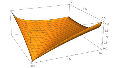
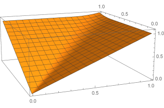
$\underline{\varphi}$	$\underline{\Theta}=\underline{\psi}$

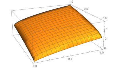
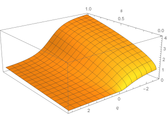
$\overline{\Theta}=\overline{\psi}=\overline{\varphi}$	$\Theta_{q^{\prime}}=\psi_{q^{\prime}}=\varphi_{q^{\prime}}$

Figure 5.1: Illustration of $\underline{\varphi}$, $\underline{\psi}=\underline{\Theta}$, $\overline{\Theta}=\overline{\psi}=\overline{\varphi}$, and $\Theta_{q^{\prime}}=\psi_{q^{\prime}}=\varphi_{q^{\prime}}$ for $\rho=0.9$. It can be observed from these figures that $\underline{\Theta}=\underline{\psi}$ is convex, $\overline{\Theta}=\overline{\psi}=\overline{\varphi}$ is concave, and $\Theta_{q^{\prime}}=\psi_{q^{\prime}}=\varphi_{q^{\prime}}$ is convex for $q\geq 1$ and convex for $q<1$. The equalities and convexity and concavity mentioned here have been shown in [39].

By observing that $\underline{\Theta},\overline{\Theta},\Theta_{q}$ are respectively the optimal exponents for the noise stability and $q$-stability (see Sections 4.2 and 4.3), it is not difficult to show the following properties of them. The proof is given in Appendix G.

Lemma 12.

For a distribution $P_{XY}$ on the product of two finite alphabets, define $\alpha_{\min}:=-\log\max_{x}P_{X}(x)$ and $\beta_{\min}:=-\log\max_{y}P_{Y}(y)$. Then for $\alpha,\beta,s,t\geq 0$ such that $\alpha+s\leq\alpha_{\min},\beta+t\leq\beta_{\min}$, we have

$$\underline{\Theta}(\alpha+s,\beta+t)-\underline{\Theta}(\alpha,\beta) \leq s+t$$ (5.6)

$$\overline{\Theta}(\alpha+s,\beta+t)-\overline{\Theta}(\alpha,\beta) \geq s+t$$ (5.7)

$$\Theta_{q^{\prime}}(\alpha+s)-\Theta_{q^{\prime}}(\alpha) \leq s\;\textrm{ for }q\geq 1$$ (5.8)

$$\Theta_{q^{\prime}}(\alpha+s)-\Theta_{q^{\prime}}(\alpha) \geq s\;\textrm{ for }q\in(0,1).$$ (5.9)

In particular, for the doubly symmetric binary distribution, (5.6)-(5.9) hold for all $\alpha,\beta\in[0,1]$ and $0\leq s\leq 1-\alpha,0\leq t\leq 1-\beta$.

Lemma 13.

For the doubly symmetric binary distribution, we have $\Theta_{r}=\breve{\varphi}_{r}$ for $r\geq 1$, and $\Theta_{r}=\invbreve{\varphi}_{r}$ for $r<0$.

Proof.

Here we only prove $\Theta_{r}=\invbreve{\varphi}_{r}$ for $r<0$. The other equality follows similarly. By Lemma 9, for the doubly symmetric binary distribution, for $r<0$,

$$\Theta_{r}(\alpha)=\max_{s\leq\alpha}\invbreve{\varphi}_{r}(s).$$ (5.10)

By Lemma 12, the supergradient of $\Theta_{r}$ is not smaller than $1$. If $\invbreve{\varphi}_{r}$ is decreasing on an interval, then by (5.10), $\Theta_{r}$ is constant on that interval, which contradicts with that the supergradient of $\Theta_{r}$ is not smaller than $1$. Hence, $\invbreve{\varphi}_{r}$ is nondecreasing. This implies that $\Theta_{r}=\invbreve{\varphi}_{r}.$ ∎

For the doubly symmetric binary distribution, by Theorems 1 and 3 and Lemma 12, we obtain the following corollaries.

Corollary 7 (Strong Brascamp–Lieb Inequalities for Binary Distributions with $\hat{p}=\hat{q}=1$ (Two-Function Version)).

Let $\alpha,\beta\in[0,1]$. Consider the doubly symmetric binary distribution in (5.1). Then the following hold.

1. For $p,q\in[1,\infty]$, we have

   $$\langle f,g\rangle \leq e^{-n(\min_{\alpha\leq s\leq 1,\beta\leq t\leq 1}\breve{\varphi}(s,t)-\frac{s}{p}-\frac{t}{q})}\|f\|_{p}\|g\|_{q}$$ (5.11)

   for all $f:\mathcal{X}^{n}\to[0,\infty),g:\mathcal{Y}^{n}\to[0,\infty)$ satisfying $\frac{1}{n}\operatorname{Ent}_{p,1}(f)\geq\alpha$ and $\frac{1}{n}\operatorname{Ent}_{q,1}(g)\geq\beta$.

2. For $p,q\in(0,1]$, we have

   $$\langle f,g\rangle \geq e^{-n(\max_{0\leq s\leq\alpha,0\leq t\leq\beta}\invbreve{\varphi}(s,t)-\frac{s}{p}-\frac{t}{q})}\|f\|_{p}\|g\|_{q}$$ (5.12)

   for all $f:\mathcal{X}^{n}\to[0,\infty),g:\mathcal{Y}^{n}\to[0,\infty)$ satisfying $\frac{1}{n}\operatorname{Ent}_{p,1}(f)\leq\alpha$ and $\frac{1}{n}\operatorname{Ent}_{q,1}(g)\leq\beta$.

3. Moreover, for given $(p,q,\alpha,\beta)$ with $\alpha,\beta\in(0,1)$, the two inequalities above are exponentially sharp.

Proof.

By Lemma 12, all the subgradients $(\lambda,\mu)$ of $\underline{\Theta}$ satisfy $\lambda,\mu\leq 1$. By definition, $\underline{\Theta}(\alpha,\beta)=\min_{\alpha\leq s\leq 1,\beta\leq t\leq 1}\breve{\varphi}(s,t)$, which implies that all the subgradients $(\lambda,\mu)$ of $\breve{\varphi}$ also satisfy $\lambda,\mu\leq 1$. By this property and Theorem 1 with $p,q$ set to $1$ (so that $\hat{p},\hat{q}$ can be equal to $\pm\infty$), we have (5.11). (Note that $p,q$ in (5.11) correspond to $\hat{p},\hat{q}$ in Theorem 1.) By Theorem 6, the inequality in (5.11) is exponentially sharp.

Inequality in (5.12) follows directly from Theorem 3. The exponential sharpness follows by Theorem 7. ∎

Similarly to the corollary above, we have the following corollary.

Corollary 8 (Strong Brascamp–Lieb Inequality for Binary Distributions with $\hat{p}=1$ (Single-Function Version)).

Let $\alpha\in[0,1]$. Consider the doubly symmetric binary distribution in (5.1). Then the following hold.

1. For $p\in[1,\infty],q\in[1,\infty)$, we have

   $$\|P_{X|Y}^{\otimes n}(f)\|_{q} \leq e^{-n(\min_{\alpha\leq s\leq 1}\breve{\varphi}_{q^{\prime}}(s)-\frac{s}{p})}\|f\|_{p}$$ (5.13)

   for all $f:\mathcal{X}^{n}\to[0,\infty)$ satisfying $\frac{1}{n}\operatorname{Ent}_{p,1}(f)\geq\alpha$.

2. For $p\in(0,1],q\in(-\infty,1)\backslash\{0\}$, we have

   $$\|P_{X|Y}^{\otimes n}(f)\|_{q} \geq e^{-n(\max_{0\leq s\leq\alpha}\invbreve{\varphi}_{q^{\prime}}(s)-\frac{s}{p})}\|f\|_{p}$$ (5.14)

   for all $f:\mathcal{X}^{n}\to[0,\infty)$ satisfying $\frac{1}{n}\operatorname{Ent}_{p,1}(f)\leq\alpha$.

3. Moreover, for given $(p,q,\alpha)$ with $\alpha\in(0,1)$, the two inequalities above are exponentially sharp.

If $p\in[p^{*},\infty],q\in[1,\infty)$ where $\frac{1}{p^{*}}$ denotes a subgradient of $\breve{\varphi}_{q^{\prime}}$ at the point $\alpha$, then the minimum in the RHS of (5.13) is attained at $s=\alpha$. Similarly, if $p\in(0,p^{*}],q\in(-\infty,1)\backslash\{0\}$ where $\frac{1}{p^{*}}$ denotes a supergradient of $\invbreve{\varphi}_{q^{\prime}}$ at the point $\alpha$, then the maximum in the RHS of (5.14) is attained at $s=\alpha$.

In a recent work [39], we have shown that for the doubly symmetric binary distribution, $\underline{\psi}$ and $\varphi_{r}$ with $r\geq 1$ are nondecreasing and convex, and $\overline{\varphi}$, $\varphi_{r}$ with $r<1,r\neq 0$ are nondecreasing and concave, which imply that

$$\underline{\Theta}=\underline{\psi}\leq\underline{\varphi},\quad\overline{\Theta}=\overline{\psi}=\overline{\varphi},\quad\Theta_{r}=\psi_{r}=\varphi_{r}.$$

Hence, the functions $\invbreve{\varphi},\breve{\varphi}_{q^{\prime}},\invbreve{\varphi}_{q^{\prime}}$ appearing in (5.12)-(5.14) can be respectively replaced by $\overline{\varphi},\varphi_{q^{\prime}}$ and $\varphi_{q^{\prime}}$. As for (5.11), since $p,q\geq 1$ is assumed, $\breve{\varphi}$ in (5.11) can be replaced by $\underline{\Theta}$, and hence can be also replaced by $\underline{\varphi}$. In other words, the time-sharing random variables can be removed for the exponents at the RHSs of (5.11)-(5.14). These further imply that the exponential sharpness of (5.11)-(5.14) is attained by the indicators of Hamming spheres (without time-sharing). Specifically, the exponents of the two sides of (5.11) coincide asymptotically as $n\to\infty$ if we choose $f,g$ as a pair of certain concentric Hamming spheres, and the exponents of the two sides of (5.12) coincide asymptotically if we choose $f,g$ as a pair of certain anti-concentric Hamming spheres. The exponents of the two sides of (5.13) with $q\in[1,\infty)$, as well as the exponents of the two sides of (5.14) with $q\in(-\infty,1)\backslash\{0\}$, respectively coincide asymptotically if we choose $f$ as certain Hamming spheres. These results in fact correspond to a conjecture of Polyansky on the forward strong Brascamp–Lieb inequality [6] and a conjecture on the reverse version. As mentioned in [6], Polyansky’s conjecture was already solved by himself in an unpublished paper [40]. Here, we independently resolve Polyansky’s conjecture and its counterpart on the reverse strong Brascamp–Lieb inequality.

The inequality in (5.13) immediately implies the following forward version of strong hypercontractivity inequality. Given $\alpha\in[0,1]$ and $q>1$, denote $p^{*}$ as the minimum $p$ such that $\min_{\alpha\leq s\leq 1}\varphi_{q^{\prime}}(s)-\frac{s}{p}=0$. Since $\varphi_{q^{\prime}}$ is a convex function and $\varphi_{q^{\prime}}(0)=0$, indeed, it holds that $1/p^{*}=\varphi_{q^{\prime}}(\alpha)/\alpha$.

Corollary 9.

For $\alpha\in(0,1)$, $q\in[1,\infty)$, and any $p\geq p^{*}$ with $1/p^{*}=\varphi_{q^{\prime}}(\alpha)/\alpha$, we have

$$\|P_{X|Y}^{\otimes n}(f)\|_{q} \leq\|f\|_{p}$$ (5.15)

for all $f:\mathcal{X}^{n}\to[0,\infty)$ satisfying $\frac{1}{n}\operatorname{Ent}_{p,1}(f)\geq\alpha$.

6 Generalization to Original BL Inequalities

Consider a tuple $(\pi_{XY},\mu_{X},\mu_{Y})$, where $\pi_{XY}$ is a $\sigma$-finite nonnegative measure on $(\mathcal{X}\times\mathcal{Y},\mathbb{B}_{\mathcal{X}}\otimes\mathbb{B}_{\mathcal{Y}})$, and $\mu_{X},\mu_{Y}$ are two $\sigma$-finite nonnegative measures respectively on $(\mathcal{X},\mathbb{B}_{\mathcal{X}})$ and $(\mathcal{Y},\mathbb{B}_{\mathcal{Y}})$. Here $\mu_{X},\mu_{Y}$ are not necessarily to be the marginals of $\pi_{XY}.$ We redefine $\langle f,g\rangle$, $\|f\|_{p}$, and $\|g\|_{q}$ respectively with respect to $\pi_{XY},\mu_{X},\mu_{Y}$. Then, the forward BL inequality corresponds to the original BL inequality studied in [1], but the reverse BL inequality in (1.2) is different from the one introduced in [2]. In fact, both of them generalize the case in which $\mu_{X},\mu_{Y}$ are the marginals of $\pi_{XY}.$

For simplicity, the condition $\pi_{X}\ll\mu_{X},\pi_{Y}\ll\mu_{Y}$ is assumed. This does not lose any generality, due to the following argument. If $\pi_{X}\centernot{\ll}\mu_{X}$, then we can write $\pi_{X}=\bar{\pi}_{X}+\hat{\pi}_{X}$ where $\bar{\pi}_{X}\ll\mu_{X}$ and $\hat{\pi}_{X}\perp\mu_{X}$. By definition, there is a measurable set $A$ such that $\mu_{X}(A^{c})=0$ and $\hat{\pi}_{X}(A)=0$. So, we can also write $f$ as $f=f1_{A}+f1_{A^{c}}$. Note that $\operatorname{Ent}_{p,\hat{p}}(f)$ only depends on the part $f1_{A}$ of $f$, and is independent of the other part. Hence, $\operatorname{Ent}_{p,\hat{p}}(f)$ remains unchanged if we rechoose $f=f1_{A}+c1_{A^{c}}.$ For this new function, $\langle f,g\rangle=\langle f1_{A},g\rangle+c\langle 1_{A^{c}},g\rangle$, which tends to infinity as $c\to\infty$. This implies $\underline{\Lambda}_{p,q,\hat{p},\hat{q}}(\alpha,\beta|\pi_{XY},\mu_{X},\mu_{Y})=-\infty$. As for the reverse part $\overline{\Lambda}_{p,q,\hat{p},\hat{q}}(\alpha,\beta)$, if $\pi_{X}\centernot{\ll}\mu_{X}$, by the argument above, without loss of optimality, one can restrict $f$ to be $f1_{A}$. If $\pi_{X}(A)=0$, then $\langle f,g\rangle=0$, which implies $\overline{\Lambda}_{p,q,\hat{p},\hat{q}}(\alpha,\beta|\pi_{XY},\mu_{X},\mu_{Y})=\infty$. Otherwise, we can denote the conditional distribution $\pi_{XY|A}$ of $\pi_{XY}$ on $A\times\mathcal{Y}$ as

$$\pi_{XY|A}:B\in\mathbb{B}_{\mathcal{X}}\otimes\mathbb{B}_{\mathcal{Y}}\mapsto\frac{\pi_{XY}(B\cap(A\times\mathcal{Y}))}{\pi_{X}(A)}.$$

Obviously, the marginal of $\pi_{XY|A}$ on $\mathcal{X}$ is $\pi_{X|A}:B\in\mathbb{B}_{\mathcal{X}}\mapsto\frac{\pi_{X}(B\cap A)}{\pi_{X}(A)}=\frac{\bar{\pi}_{X}(B\cap A)}{\bar{\pi}_{X}(A)}$. Hence, $\pi_{X|A}\ll\mu_{X}$. On the other hand,

$$\overline{\Lambda}_{p,q,\hat{p},\hat{q}}(\alpha,\beta|\pi_{XY},\mu_{X},\mu_{Y})=\overline{\Lambda}_{p,q,\hat{p},\hat{q}}(\alpha,\beta|\pi_{XY|A},\mu_{X},\mu_{Y})-\log\pi_{X}(A),$$

which implies that determining $\overline{\Lambda}_{p,q,\hat{p},\hat{q}}$ for $(\pi_{XY},\mu_{X},\mu_{Y})$ is equivalent to determining $\overline{\Lambda}_{p,q,\hat{p},\hat{q}}$ for $(\pi_{XY|A},\mu_{X},\mu_{Y})$. Hence, $\pi_{X}\ll\mu_{X},\pi_{Y}\ll\mu_{Y}$ can be assumed.

By checking our proofs, one can verify that for the case of $\pi_{X}\ll\mu_{X},\pi_{Y}\ll\mu_{Y}$, all the inequalities derived in Sections 2-4 still hold for this general setting, but they require to be slightly modified. For this general case, $\operatorname{Ent}_{p,\hat{p}}(f)=D_{\hat{p}/p}(Q_{X}\|\mu_{X})$ still holds, but the Rényi divergence here is required to extend to the one of a probability from a $\sigma$-finite nonnegative measure. More specifically, the Rényi divergence of a probability measure $Q$ from a $\sigma$-finite nonnegative measure $\mu$ on the same measurable space is still defined as $D_{s}(Q\|\mu):=\frac{1}{s-1}\log\int(\frac{\mathrm{d}Q}{\mathrm{d}\nu})^{s}(\frac{\mathrm{d}\mu}{\mathrm{d}\nu})^{1-s}\mathrm{d}\nu$ for $s\in\mathbb{R}\backslash\{0,1\}$ and a $\sigma$-finite nonnegative measure $\nu$ such that $Q,\mu\ll\nu$ (in fact, the value of $D_{s}(Q\|\mu)$ is independent of the choice of $\nu$). For $s\in\{0,1,\pm\infty\}$, the Rényi divergence of order $s$ is still defined by the continuous extension. In particular, the formula for the relative entropy (i.e., the case $s=1$) can be found in Remark 9 in Appendix A. In fact, this general version of the Rényi divergence can be seen as the negative Rényi entropy of $Q$ with respect to the reference measure $\mu$. It still admits the following variational formula (see e.g. Lemma 14 in Appendix A):

$$D_{s}(Q\|\mu)=\frac{1}{1-s}\inf_{R}\{sD(R\|Q)+(1-s)D(R\|\mu)\},$$ (6.1)

where the infimum is still taken over probability measures $R$. By this formula, given $Q,\mu$, the Rényi divergence $D_{s}(Q\|\mu)$ is still nondecreasing in its order $s\in[-\infty,\infty]$. Similarly to Lemma 1, one can also prove the continuity of $D_{s}(Q\|\mu)$ in $s\in\{s:|D_{s}(Q\|\mu)|<\infty\}$. However, unlike the case of probability measure $\mu$, in general, for a $\sigma$-finite nonnegative measure $\mu$, $D_{s}(Q\|\mu)$ is not nonnegative anymore for $s\geq 0$, and also not nonpositive anymore for $s<0$. Based on this general definitions of the Rényi divergence and the relative entropy, all the inequalities derived in Sections 2-4 still hold if we replace $(P_{XY},P_{X},P_{Y})$ with the tuple $(\pi_{XY},\mu_{X},\mu_{Y})$. Note that all the optimizations involved in these results are still taken over probability measures. Furthermore, it should be noted that for the single-function version of BL inequalities and the theorems on the $q$-stability, we should additionally assume $\mu_{Y}=\pi_{Y}$, so that the equivalences in (3.8) and (3.9) are still valid for the new setting.

In addition, the proofs of the exponential tightness of the inequalities derived in Sections 2-4 requires the large deviation theory, more specifically, Sanov’s theorem. If $\pi_{XY},\mu_{X},\mu_{Y}$ are finite measures, then we can normalize them to probability measures. In this case, Sanov’s theorem for the probability measures still works. However, if $\pi_{XY},\mu_{X},\mu_{Y}$ are infinite (but $\sigma$-finite) measures, our proofs require a version of Sanov’s theorem for infinite measures. In fact, the generalization of Sanov’s theorem to infinite measures was already investigated in [41], but for a so-called fine topology, instead of the weak topology. The exponential tightness of the inequalities derived in Sections 2-4 for infinite measures remains to be investigated in the future.

Appendix A Proof of Proposition 2

To prove Proposition 2, we need the following lemma.

Lemma 14.

Let $P_{i},i\in[n]$ be $n$ probability measures on $\mathcal{X}$ and $\mu$ be a $\sigma$-finite nonnegative measure on $\mathcal{X}$ such that all $P_{i}\ll\mu,i\in[n]$. Let $s_{i},i\in[n]$ be $n$ real numbers such that $\sum_{i=1}^{n}s_{i}=1$. Let $c:\mathcal{X}\to[-\infty,\infty]$ be a measurable function. Denote $\beta:=\int e^{-c}\prod_{i=1}^{n}(\frac{\mathrm{d}P_{i}}{\mathrm{d}\mu})^{s_{i}}\mathrm{d}\mu$. Then we have

$$-\log\beta=\inf_{Q}\sum_{i=1}^{n}s_{i}D(Q\|P_{i})+\int c\,\mathrm{d}Q,$$ (A.1)

where the conventions that $0\cdot\infty=0$, and $0^{s}=\infty$ for $s<0$, and $1$ for $s=0$ are adopted, according to Convention 1, the infimization in the RHS of (A.1) is over all probability measures $Q$ on $\mathcal{X}$ such that $D(Q\|P_{i})<\infty,\forall i\in[n]$ and $\int|c|\,\mathrm{d}Q<\infty$. Moreover, if $0<\beta<\infty$, $D(Q^{*}\|P_{i})<\infty,\forall i\in[n]$, and $\int|c|\,\mathrm{d}Q^{*}<\infty$, where $Q^{*}$ is a probability measure with the density

$$\frac{\mathrm{d}Q^{*}}{\mathrm{d}\mu}=\frac{e^{-c}}{\beta}\prod_{i=1}^{n}(\frac{\mathrm{d}P_{i}}{\mathrm{d}\mu})^{s_{i}},$$ (A.2)

then the infimization in the RHS of (A.1) is uniquely attained by $Q^{*}$.

Remark 8.

In fact, from the definition, $\beta$ is independent of the reference measure $\mu$, which can be also seen from (A.1).

Remark 9.

The probability measures $P_{i},i\in[n]$ can be relaxed to any $\sigma$-finite nonnegative measures. For this case, the relative entropy of a probability measure $Q$ from a $\sigma$-finite nonnegative measure $\pi$ on the same measurable space is still defined as $D(Q\|\pi):=\int\log(\frac{\mathrm{d}Q}{\mathrm{d}\pi})\mathrm{d}Q$ if $Q\ll\pi$ and the integral exists, and infinity otherwise. Moreover, the infimum in (A.1) is still taken over probability measures.

Remark 10.

Special cases of this lemma were provided in [42, 43, 4]. The finite alphabet version can be proven by the Lagrange multiplier method. The proof here is based on the non-negativity of the relative entropy, which is essentially due to Csiszár and Matus [44] and also used in [4, 20].

Proof.

We first consider the case $0<\beta<\infty$. For $0<a<b<\infty$, define

$$\mathcal{A}_{a,b}:=\Big{\{}x:\frac{\mathrm{d}P_{i}}{\mathrm{d}\mu}(x),c(x)\in(a,b),\forall i\in[n]\Big{\}}.$$

Observe that for any $Q\ll\mu$ concentrated on $\mathcal{A}_{a,b}$, we have $D(Q\|P_{i})<\infty,\forall i\in[n]$, $\int|c|\,\mathrm{d}Q<\infty$, and moreover,

$$\sum_{i=1}^{n}s_{i}D(Q\|P_{i})+\int c\,\mathrm{d}Q+\log\beta_{a,b} =D(Q\|Q_{a,b}^{*})\geq 0,$$

where $\beta_{a,b}:=\int_{\mathcal{A}_{a,b}}\prod_{i=1}^{n}(\frac{\mathrm{d}P_{i}}{\mathrm{d}\mu})^{s_{i}}\mathrm{d}\mu$, and $Q_{a,b}^{*}$ is a probability measure with the density

$$\frac{\mathrm{d}Q_{a,b}^{*}}{\mathrm{d}\mu}:=\frac{1_{\mathcal{A}_{a,b}}e^{-c}\prod_{i=1}^{n}(\frac{\mathrm{d}P_{i}}{\mathrm{d}\mu})^{s_{i}}}{\beta_{a,b}}.$$

The equality above holds if $Q=Q_{a,b}^{*}$. Hence,

$$-\log\beta_{a,b}=\inf_{Q:\,Q(\mathcal{A}_{a,b}^{c})=0}\sum_{i=1}^{n}s_{i}D(Q\|P_{i})+\int c\,\mathrm{d}Q,$$

by Convention 1, the infimum is taken over all $Q$ such that $Q(\mathcal{A}_{a,b}^{c})=0$, $D(Q\|P_{i})<\infty,\forall i\in[n],\int|c|\,\mathrm{d}Q<\infty$. Taking infimization over $0<a<b<\infty$ for both sides above and applying the monotone convergence theorem, we have

$$-\log\beta=\inf_{0<a<b<\infty}\inf_{Q:\,Q(\mathcal{A}_{a,b}^{c})=0}\sum_{i=1}^{n}s_{i}D(Q\|P_{i})+\int c\,\mathrm{d}Q,$$

which implies

$$-\log\beta\geq\inf_{Q}\sum_{i=1}^{n}s_{i}D(Q\|P_{i})+\int c\mathrm{d}Q.$$ (A.3)

On the other hand, for any $Q$ such that $D(Q\|P_{i})<\infty,\forall i\in[n]$ and $\int|c|\mathrm{d}Q<\infty$, we have

$$\sum_{i=1}^{n}s_{i}D(Q\|P_{i})+\int c\mathrm{d}Q+\log\beta =D(Q\|Q^{*})\geq 0,$$ (A.4)

where $Q^{*}$ is defined in (A.2) and its existence follows by the assumption $0<\beta<\infty$. It is easy to see that the equality for the inequality above holds if $Q=Q^{*}$, $D(Q^{*}\|P_{i})<\infty,\forall i\in[n]$, and $\int|c|\mathrm{d}Q^{*}<\infty$. Therefore, combining (A.3) and (A.4) yields (A.1).

We next consider the case $\beta=\infty$. For this case, it is easy to check that (A.3) still holds. Hence, both sides of (A.1) are $-\infty$.

We lastly consider the case $\beta=0$. For this case, $e^{-c}\prod_{i=1}^{n}(\frac{\mathrm{d}P_{i}}{\mathrm{d}\mu})^{s_{i}}=0$ holds $\mu$-a.e. Hence, for any $Q$, it holds that $\int|c|\mathrm{d}Q^{*}=\infty$ or there exists at least one $i\in[n]$ such that $s_{i}>0$ and $D(Q\|P_{i})=\infty$. Hence, the infimization at the RHS of (A.1) is taken over the empty set. Hence, both sides of (A.1) are $\infty$. This completes the proof of Lemma 14. ∎

We may assume, by homogeneilty, that $\|f\|_{p}=\|g\|_{q}=1$. Observe that all the integrals involved in $\|f\|_{p},\|g\|_{q}$, $\operatorname{Ent}_{p,\hat{p}}(f)$, $\operatorname{Ent}_{q,\hat{q}}(g),\langle f,g\rangle$ can be written as the ones with respect to $P_{XY}$. Hence, we can choose $P_{XY}$ as a reference measure. Then, without loss of generality, we can write

$$f^{p}=\frac{\mathrm{d}Q_{X}}{\mathrm{d}P_{X}}=\frac{\mathrm{d}(Q_{X}P_{Y|X})}{\mathrm{d}P_{XY}}\qquad g^{q}=\frac{\mathrm{d}Q_{Y}}{\mathrm{d}P_{Y}}=\frac{\mathrm{d}(Q_{Y}P_{X|Y})}{\mathrm{d}P_{XY}},$$

for some probability measures $Q_{X}\ll P_{X},Q_{Y}\ll P_{Y}$. Moreover, we require $f<\infty$. Hence, $Q_{X}\ll\gg P_{X}$ if $p<0$. Similarly, $Q_{Y}\ll\gg P_{Y}$ if $q<0$.

By this choice of $f,g$, we have

$$\operatorname{Ent}_{p,\hat{p}}(f) =-\frac{p}{p-\hat{p}}\log\int(\frac{\mathrm{d}Q_{X}}{\mathrm{d}P_{X}})^{\hat{p}/p}\mathrm{d}P_{X}=D_{\hat{p}/p}(Q_{X}\|P_{X}).$$ (A.5)

To ensure that $D_{{\hat{p}}/{p}}(Q_{X}\|P_{X})$ is finite, for the case $p>0>\hat{p}$, we still require $Q_{X}\ll\gg P_{X}$. Hence, $Q_{X}\ll P_{X}$ if $p>0,\hat{p}\geq 0$; otherwise, $Q_{X}\ll\gg P_{X}$. Similarly, $Q_{Y}\ll P_{Y}$ if $q>0,\hat{q}\geq 0$; otherwise, $Q_{Y}\ll\gg P_{Y}$.

In addition, we also have that

$$-\log\langle f,g\rangle =-\log\int(\frac{\mathrm{d}(Q_{X}P_{Y|X})}{\mathrm{d}P_{XY}})^{1/p}(\frac{\mathrm{d}(Q_{Y}P_{X|Y})}{\mathrm{d}P_{XY}})^{1/q}\mathrm{d}P_{XY}$$ (A.6)

$$=\inf_{R_{XY}}\{D(R_{XY}\|P_{XY})+\frac{1}{p}D(R_{X}\|Q_{X})-\frac{1}{p}D(R_{X}\|P_{X})+\frac{1}{q}D(R_{Y}\|Q_{Y})-\frac{1}{q}D(R_{Y}\|P_{Y})\}$$ (A.7)

$$=\phi(Q_{X},Q_{Y}|P_{XY}),$$ (A.8)

where (A.7) follows by Lemma 14, and moreover, in (A.7), the infimization is taken over all $R_{XY}$ such that all the relative entropies appearing in the objective function are finite.

Substituting (A.5) and (A.8) into the definitions of $\underline{\Lambda}_{p,q,\hat{p},\hat{q}}(\alpha,\beta)$ and $\overline{\Lambda}_{p,q,\hat{p},\hat{q}}(\alpha,\beta)$ yields Theorem 2.

Appendix B Proof of Theorem 1

B.1 Forward Case

Our proof consists of two parts: one-shot bound and singleletterization.

B.1.1 One-shot Bound

We first consider the case $n=1$. Denote $\lambda=\hat{p}/p,\mu=\hat{q}/q$. Define

$$\psi(R_{XY}) =D(R_{XY}\|P_{XY})-\frac{1}{p}D(R_{X}\|P_{X})-\frac{1}{q}D(R_{Y}\|P_{Y})$$

$$\qquad+\inf_{\begin{subarray}{c}Q_{X}:D_{\lambda}(Q_{X}\|P_{X})=\alpha\end{subarray}}\frac{1}{p}D(R_{X}\|Q_{X})+\inf_{\begin{subarray}{c}Q_{Y}:D_{\mu}(Q_{Y}\|P_{Y})=\beta\end{subarray}}\frac{1}{q}D(R_{Y}\|Q_{Y}).$$

Then $\underline{\Lambda}_{p,q,\hat{p},\hat{q}}(\alpha,\beta)=\inf_{R_{XY}}\psi(R_{XY})+\frac{\alpha}{p}+\frac{\beta}{q}.$ We will prove

$$\xi:=\frac{1}{p}(\alpha-D(R_{X}\|P_{X}))+\inf_{\begin{subarray}{c}Q_{X}:D_{\lambda}(Q_{X}\|P_{X})=\alpha\end{subarray}}\frac{1}{p}D(R_{X}\|Q_{X}) \geq\eta_{p,\hat{p}}(\alpha,D(R_{X}\|P_{X})),$$ (B.1)

which, by symmetry, implies that a similar inequality holds for $P_{Y}$, and further implies that

$$\underline{\Lambda}_{p,q,\hat{p},\hat{q}}(\alpha,\beta) \geq\inf_{R_{XY}}D(R_{XY}\|P_{XY})+\eta_{p,\hat{p}}(\alpha,D(R_{X}\|P_{X}))+\eta_{q,\hat{q}}(\beta,D(R_{Y}\|P_{Y})).$$ (B.2)

I. We first assume $p>0,\hat{p}\geq 0$.

1) We first consider the case $\lambda\in(0,\infty]\backslash\{1\}$. By Lemma 14,

$$D_{\lambda}(Q_{X}\|P_{X})=\frac{1}{1-\lambda}\inf_{R_{X}}\{\lambda D(R_{X}\|Q_{X})+(1-\lambda)D(R_{X}\|P_{X})\}.$$ (B.3)

Hence, for any $R_{X}$,

$$\inf_{\begin{subarray}{c}Q_{X}:D_{\lambda}(Q_{X}\|P_{X})=\alpha\end{subarray}}\frac{1}{p}D(R_{X}\|Q_{X})\geq\frac{1-\lambda}{\hat{p}}(\alpha-D(R_{X}\|P_{X})).$$ (B.4)

Combining this with the nonnegtivity of relative entropies yields that the left-hand side (LHS) above is lower bounded by $[\frac{1-\lambda}{\hat{p}}(\alpha-D(R_{X}\|P_{X}))]^{+}$, where $[x]^{+}:=x\vee 0$. Hence,

$$\xi \geq\frac{1}{p}(\alpha-D(R_{X}\|P_{X}))+[\frac{1-\lambda}{\hat{p}}(\alpha-D(R_{X}\|P_{X}))]^{+}=\eta_{p,\hat{p}}(\alpha,D(R_{X}\|P_{X})).$$ (B.5)

2) We next consider the case $\lambda=0$. Observe that for any feasible $(R_{XY},Q_{X})$, we have $R_{X}\ll Q_{X}\ll P_{X}$ since, otherwise, $\inf_{\begin{subarray}{c}Q_{X}:D_{0}(Q_{X}\|P_{X})=\alpha\end{subarray}}\frac{1}{p}D(R_{X}\|Q_{X})=\infty$. This means, $\alpha=D_{0}(Q_{X}\|P_{X})\leq D_{0}(R_{X}\|P_{X})\leq D(R_{X}\|P_{X})$. Therefore, by the nonnegtivity of relative entropies, we have

$$\xi \geq\begin{cases}\frac{1}{p}(\alpha-D(R_{X}\|P_{X})),&D(R_{X}\|P_{X})\geq\alpha\\ \infty,&D(R_{X}\|P_{X})<\alpha\end{cases}\;=\eta_{p,\hat{p}}(\alpha,D(R_{X}\|P_{X})).$$

3) We next consider the case $\lambda=1$. By the nonnegtivity of relative entropies, we have $\xi\geq\frac{1}{p}(\alpha-D(R_{X}\|P_{X}))=\eta_{p,\hat{p}}(\alpha,D(R_{X}\|P_{X})).$

II. For $p<0<\hat{p}$, (B.4) still holds. Hence, (B.1) holds.

III. For $\hat{p}<0<p$, by the nonnegtivity of relative entropies, we have $\xi\geq\frac{1}{p}(\alpha-D(R_{X}\|P_{X}))=\eta_{p,\hat{p}}(\alpha,D(R_{X}\|P_{X})).$

IV. For $p<0,\hat{p}\leq 0$, (B.1) holds trivially since the RHS is equal to $-\infty$.

B.1.2 Singleletterization

We next consider the singleletterization. Substituting $(\alpha,\beta,P_{XY})\leftarrow(n\alpha,n\beta,P_{XY}^{\otimes n}),$ we obtain the $n$-dimensional version:

$$\underline{\Lambda}_{p,q,\hat{p},\hat{q}}^{(n)}(\alpha,\beta) \geq\frac{1}{n}\inf_{R_{X^{n}Y^{n}}}D(R_{X^{n}Y^{n}}\|P_{XY}^{\otimes n})+\eta_{p,\hat{p}}(n\alpha,D(R_{X^{n}}\|P_{X}^{\otimes n}))$$

$$\qquad+\eta_{q,\hat{q}}(n\beta,D(R_{Y^{n}}\|P_{Y}^{\otimes n})).$$ (B.6)

By the chain rule, we have

$$D(R_{X^{n}Y^{n}}\|P_{XY}^{\otimes n}) =\sum_{i=1}^{n}D(R_{X_{i}Y_{i}|X^{i-1}Y^{i-1}}\|P_{XY}|R_{X^{i-1}Y^{i-1}})$$ (B.7)

$$D(R_{X^{n}}\|P_{X}^{\otimes n}) =\sum_{i=1}^{n}D(R_{X_{i}|X^{i-1}}\|P_{X}|R_{X^{i-1}})$$

$$D(R_{Y^{n}}\|P_{Y}^{\otimes n}) =\sum_{i=1}^{n}D(R_{Y_{i}|Y^{i-1}}\|P_{Y}|R_{Y^{i-1}}).$$

Consider the joint distribution $R_{X^{n}Y^{n}K}:=R_{X^{n}Y^{n}}\otimes\mathrm{Unif}[n]$, i.e., under this distribution, $K\sim\mathrm{Unif}[n]$ (called a random index) is independent of $(X^{n},Y^{n})$. Denote $X:=X_{K},Y:=Y_{K},U:=(X^{K-1},K),V:=(Y^{K-1},K),W:=(U,V)$. Then

$$D(R_{X^{n}Y^{n}}\|P_{XY}^{\otimes n}) =nD(R_{XY|W}\|P_{XY}|R_{W})$$

$$D(R_{X^{n}}\|P_{X}^{\otimes n}) =nD(R_{X|U}\|P_{X}|R_{U})\leq nD(R_{X|W}\|P_{X}|R_{W})$$

$$D(R_{Y^{n}}\|P_{Y}^{\otimes n}) =nD(R_{Y|V}\|P_{Y}|R_{V})\leq nD(R_{Y|W}\|P_{Y}|R_{W}),$$

where the inequalities in the last two lines follow by the fact that conditioning increasing the relative entropy. Substituting these into (B.6) and utilizing the monotonicity of $\eta_{p,\hat{p}}(\alpha,s)$ in $s$ yields that

$$\underline{\Lambda}_{p,q,\hat{p},\hat{q}}^{(n)}(\alpha,\beta) \geq\inf_{R_{XYW}}D(R_{XY|W}\|P_{XY}|R_{W})$$

$$\qquad+\eta_{p,\hat{p}}(\alpha,D(R_{X|W}\|P_{X}|R_{W}))+\eta_{q,\hat{q}}(\beta,D(R_{Y|W}\|P_{Y}|R_{W}))$$

$$=\underline{\Lambda}_{p,q,\hat{p},\hat{q}}^{*}(\alpha,\beta).$$ (B.8)

B.2 Reverse Case

Define $\overline{\Lambda}_{p,q,\hat{p},\hat{q}}^{**}(\alpha,\beta)$ as a variant of $\overline{\Lambda}_{p,q,\hat{p},\hat{q}}^{*}(\alpha,\beta)$, by removing $\sup_{Q_{W}}$ from the definition of $\overline{\Lambda}_{p,q,\hat{p},\hat{q}}^{*}(\alpha,\beta)$, and moreover, taking $Q_{W}$ to be a Dirac measure. In the following, we first consider the case $n=1$, and prove

$$\overline{\Lambda}_{p,q,\hat{p},\hat{q}}(\alpha,\beta)\leq\overline{\Lambda}_{p,q,\hat{p},\hat{q}}^{**}(\alpha,\beta).$$ (B.9)

We then prove the $n$-dimensional version

$$\overline{\Lambda}_{p,q,\hat{p},\hat{q}}^{**}(n\alpha,n\beta|P_{XY}^{\otimes n})\leq n\overline{\Lambda}_{p,q,\hat{p},\hat{q}}^{*}(\alpha,\beta).$$ (B.10)

These yield the desired result

$$\overline{\Lambda}_{p,q,\hat{p},\hat{q}}^{(n)}(\alpha,\beta)\leq\overline{\Lambda}_{p,q,\hat{p},\hat{q}}^{*}(\alpha,\beta).$$ (B.11)

Denote $\lambda=\hat{p}/p,\mu=\hat{q}/q$. Define

$$\psi(Q_{X},Q_{Y},R_{X},R_{Y}) =\mathbb{D}(R_{X},R_{Y}\|P_{XY})-\frac{1}{p}D(R_{X}\|P_{X})-\frac{1}{q}D(R_{Y}\|P_{Y})$$

$$\qquad+\frac{1}{p}D(R_{X}\|Q_{X})+\frac{1}{q}D(R_{Y}\|Q_{Y})+\frac{\alpha}{p}+\frac{\beta}{q}.$$

Then, $\phi(Q_{X},Q_{Y})+\frac{\alpha}{p}+\frac{\beta}{q}=\inf_{R_{X},R_{Y}}\psi(Q_{X},Q_{Y},R_{X},R_{Y}).$

B.2.1 One-shot Bound

We now prove (B.9). We divide our proof into several parts according to different cases:

I. $p,q>0,\hat{p},\hat{q}\geq 0$: 1) $\lambda,\mu\in(1,\infty)$ or $\lambda,\mu\in(0,1)$; 2) $\lambda=\mu=0$; 3) $\lambda=\mu=1$; 4) $\lambda=\mu=\infty$.

II. $p,q<0,\hat{p},\hat{q}\geq 0$: 1) $p,q<0<\hat{p},\hat{q}\leq\infty$; 2) $p,q<0=\hat{p}=\hat{q}$.

III. $p,q>0,\hat{p},\hat{q}<0$: 1) $p,q>0>\hat{p},\hat{q}>-\infty$; 2) $p,q>0,\hat{p},\hat{q}=-\infty$.

IV. $p,q,\hat{p},\hat{q}<0$.

V. Other cases.

The cases I-IV are “symmetric” with respect to $(p,q)$ and also with respect to $(\hat{p},\hat{q})$. For brevity, we only provide the proof for these “symmetric” cases. For the “asymmetric” case (i.e., the case V), one can prove (B.9) by “mixing” the proofs for “symmetric” cases, since the “asymmetric” case can be seen as a mixture of the “symmetric” cases.

I. We first assume $p,q>0,\hat{p},\hat{q}\geq 0$, and prove (B.9) for this case.

1) We first consider the case $\lambda,\mu\in(1,\infty)$. Define $R_{X}^{*}$ as the distribution with density

$$\frac{\mathrm{d}R_{X}^{*}}{\mathrm{d}P_{X}}=\frac{(\frac{\mathrm{d}Q_{X}}{\mathrm{d}P_{X}})^{\lambda}}{\int(\frac{\mathrm{d}Q_{X}}{\mathrm{d}P_{X}})^{\lambda}\mathrm{d}P_{X}}.$$ (B.12)

The existence of $R_{X}^{*}$ follows by the requirement $D_{\lambda}(Q_{X}\|P_{X})=\alpha<\infty$. Define $R_{Y}^{*}$ similarly. We first assume that $D(R_{X}^{*}\|P_{X}),D(R_{Y}^{*}\|Q_{Y})<\infty$, and later will consider the case $D(R_{X}^{*}\|P_{X})=\infty$ or $D(R_{Y}^{*}\|Q_{Y})=\infty$. It is easy to check that for $D(R_{X}^{*}\|P_{X})<\infty$, we have

$$D(R_{X}^{*}\|P_{X})+\frac{\lambda}{1-\lambda}D(R_{X}^{*}\|Q_{X})=D_{\lambda}(Q_{X}\|P_{X}),$$ (B.13)

which, combined with the monotonicity of the Rényi divergence in its order, implies that for $\lambda>1$,

$$D(Q_{X}\|P_{X})\leq D_{\lambda}(Q_{X}\|P_{X})\leq D(R_{X}^{*}\|P_{X}).$$ (B.14)

Denote $s=D(Q_{X}\|P_{X}),\hat{s}=D(R_{X}^{*}\|P_{X})$ and $t=D(Q_{Y}\|P_{Y}),\hat{t}=D(R_{Y}^{*}\|P_{Y})$. Then under the constraints $D_{\lambda}(Q_{X}\|P_{X})=\alpha,D_{\mu}(Q_{Y}\|P_{Y})=\beta$, we have

$$s\leq\alpha\leq\hat{s},\quad t\leq\beta\leq\hat{t}.$$ (B.15)

Hence, we have

$$\phi(Q_{X},Q_{Y})+\frac{\alpha}{p}+\frac{\beta}{q} \leq\min_{R_{X}\in\{R_{X}^{*},Q_{X}\},R_{Y}\in\{R_{Y}^{*},Q_{Y}\}}\psi(Q_{X},Q_{Y},R_{X},R_{Y})$$ (B.16)

$$\leq\hat{\phi}(Q_{X},Q_{Y},R_{X}^{*},R_{Y}^{*}),$$ (B.17)

where

$$\hat{\phi}(Q_{X},Q_{Y},R_{X},R_{Y}) :=\min\biggl{\{}\mathbb{D}(R_{X},R_{Y}\|P_{XY})+\frac{\alpha-\hat{s}}{\hat{p}}+\frac{\beta-\hat{t}}{\hat{q}},\;\mathbb{D}(R_{X},Q_{Y}\|P_{XY})+\frac{\alpha-\hat{s}}{\hat{p}}+\frac{\beta-t}{q},$$

$$\qquad\mathbb{D}(Q_{X},R_{Y}\|P_{XY})+\frac{\alpha-s}{p}+\frac{\beta-\hat{t}}{\hat{q}},\>\mathbb{D}(Q_{X},Q_{Y}\|P_{XY})+\frac{\alpha-s}{p}+\frac{\beta-t}{q}\biggr{\}},$$

and in (B.20), (B.13) was used to eliminate the terms $D(R_{X}^{*}\|Q_{X}),D(R_{Y}^{*}\|Q_{Y})$. Then, relaxing $Q_{X},Q_{Y},R_{X}^{*},R_{Y}^{*}$ to arbitrary distributions satisfying (B.15), we obtain

$$\overline{\Lambda}_{p,q,\hat{p},\hat{q}}(\alpha,\beta) \leq\sup_{\begin{subarray}{c}s\leq\alpha\leq\hat{s},\,t\leq\beta\leq\hat{t}\end{subarray}}\sup_{\begin{subarray}{c}Q_{X},Q_{Y},R_{X},R_{Y}:\\ D(Q_{X}\|P_{X})=s,D(Q_{Y}\|P_{Y})=t\\ D(R_{X}\|P_{X})=\hat{s},D(R_{Y}\|P_{Y})=\hat{t}\end{subarray}}\hat{\phi}(Q_{X},Q_{Y},R_{X},R_{Y})=\overline{\Lambda}_{p,q,\hat{p},\hat{q}}^{**}(\alpha,\beta).$$ (B.18)

We now consider the case $D(R_{X}^{*}\|P_{X})=\infty$ or $D(R_{Y}^{*}\|Q_{Y})=\infty$. Here we only provide a proof for the case of $D(R_{X}^{*}\|P_{X})=D(R_{Y}^{*}\|Q_{Y})=\infty$. The case of $D(R_{X}^{*}\|P_{X})<D(R_{Y}^{*}\|Q_{Y})=\infty$ and the case of $D(R_{Y}^{*}\|Q_{Y})<D(R_{X}^{*}\|P_{X})=\infty$ can be proven similarly. If $D(R_{X}^{*}\|P_{X})=\infty$, we replace $R_{X}^{*}$ above as the distribution $R_{X}^{(r)}$ with density w.r.t. $P_{X}$ being

$$\frac{\mathrm{d}R_{X}^{(r)}}{\mathrm{d}P_{X}}=\frac{(\frac{\mathrm{d}Q_{X}}{\mathrm{d}P_{X}})^{\lambda}1_{\mathcal{A}_{r}}}{\int(\frac{\mathrm{d}Q_{X}}{\mathrm{d}P_{X}})^{\lambda}1_{\mathcal{A}_{r}}\mathrm{d}P_{X}}$$ (B.19)

where $\mathcal{A}_{r}:=\{x:\frac{\mathrm{d}Q_{X}}{\mathrm{d}P_{X}}(x)<r\}$ for $r>0$. Then it is easy to verify that $D(R_{X}^{(r)}\|P_{X})<\infty$ and $D(R_{X}^{(r)}\|P_{X})\to D(R_{X}^{*}\|P_{X})=\infty$ as $r\to\infty$. Moreover, analogue to (B.13), we have

$$(1-\lambda)D(R_{X}^{(r)}\|P_{X})+\lambda D(R_{X}^{(r)}\|Q_{X})=(1-\lambda)D_{\lambda}(Q_{X}\|P_{X})+\varepsilon_{r},$$ (B.20)

where $\varepsilon_{r}\geq 0$ vanishes as $r\to\infty$. The equality above implies that $D(R_{X}^{(r)}\|Q_{X})\to\infty$ as $r\to\infty$, under the constraint $D_{\lambda}(Q_{X}\|P_{X})=\alpha$. Hence, for sufficiently large $r$, $D(R_{X}^{(r)}\|P_{X})\geq\alpha$. By redefining $\hat{s}=D(R_{X}^{(r)}\|P_{X})$, we have that (B.15) still holds. Using (B.20) to replace (B.13), we still have (B.17), but with $\hat{\phi}$ replaced by the following $\hat{\phi}_{r}$.

$$\hat{\phi}_{r}(Q_{X},Q_{Y},R_{X},R_{Y}) :=\min\biggl{\{}\mathbb{D}(R_{X},R_{Y}\|P_{XY})+\frac{\alpha-\hat{s}+\varepsilon_{r}}{\hat{p}}+\frac{\beta-\hat{t}+\varepsilon_{r}}{\hat{q}},$$

$$\qquad\mathbb{D}(R_{X},Q_{Y}\|P_{XY})+\frac{\alpha-\hat{s}+\varepsilon_{r}}{\hat{p}}+\frac{\beta-t}{q},$$

$$\qquad\mathbb{D}(Q_{X},R_{Y}\|P_{XY})+\frac{\alpha-s}{p}+\frac{\beta-\hat{t}+\varepsilon_{r}}{\hat{q}},$$

$$\qquad\mathbb{D}(Q_{X},Q_{Y}\|P_{XY})+\frac{\alpha-s}{p}+\frac{\beta-t}{q}\biggr{\}}.$$

Then, letting $r\to\infty$, we have (B.18). This completes the proof of (B.9) for the case $\lambda,\mu\in(1,\infty)$.

Since $\overline{\Lambda}_{p,q,\hat{p},\hat{q}}(\alpha,\beta)$ is symmetric w.r.t. $p,\hat{p}$ and also $q,\hat{q}$, (B.9) holds for the case $\lambda,\mu\in(0,1)$.

2) We next consider the case $\lambda=\mu=0$. By the monotonicity of the Rényi divergence in its order, $D(Q_{X}\|P_{X})\geq D_{0}(Q_{X}\|P_{X}).$ Denote $s=D(Q_{X}\|P_{X})$ and $t=D(Q_{Y}\|P_{Y})$. Then under the constraints $D_{0}(Q_{X}\|P_{X})=\alpha,D_{0}(Q_{Y}\|P_{Y})=\beta$, we have $s\geq\alpha,t\geq\beta.$ Hence, we have

$$\phi(Q_{X},Q_{Y})+\frac{\alpha}{p}+\frac{\beta}{q}\leq\mathbb{D}(Q_{X},Q_{Y}\|P_{XY})+\frac{\alpha-s}{p}+\frac{\beta-t}{q}.$$ (B.21)

Then, relaxing $Q_{X},Q_{Y}$ to be arbitrary distributions satisfying $s\geq\alpha,t\geq\beta$, we obtain

$$\overline{\Lambda}_{p,q,\hat{p},\hat{q}}(\alpha,\beta) \leq\sup_{s\geq\alpha,t\geq\beta}\sup_{\begin{subarray}{c}Q_{X},Q_{Y}:\\ D(Q_{X}\|P_{X})=s,D(Q_{Y}\|P_{Y})=t\end{subarray}}\mathbb{D}(Q_{X},Q_{Y}\|P_{XY})+\frac{\alpha-s}{p}+\frac{\beta-t}{q}$$ (B.22)

$$=\overline{\Lambda}_{p,q,\hat{p},\hat{q}}^{**}(\alpha,\beta).$$ (B.23)

3) We next consider the case $\lambda=\mu=1$. For this case, (B.21) still holds. Then, we obtain

$$\overline{\Lambda}_{p,q,\hat{p},\hat{q}}(\alpha,\beta) \leq\sup_{\begin{subarray}{c}Q_{X},Q_{Y}:\\ D(Q_{X}\|P_{X})=\alpha,D(Q_{Y}\|P_{Y})=\beta\end{subarray}}\mathbb{D}(Q_{X},Q_{Y}\|P_{XY})+\frac{\alpha-s}{p}+\frac{\beta-t}{q}$$ (B.24)

$$=\overline{\Lambda}_{p,q,\hat{p},\hat{q}}^{**}(\alpha,\beta).$$ (B.25)

4) We then consider the case $\lambda=\mu=\infty$. Suppose that $P_{X}(A)>0$ with $A:=\{x:\frac{\mathrm{d}Q_{X}}{\mathrm{d}P_{X}}(x)=\|\frac{\mathrm{d}Q_{X}}{\mathrm{d}P_{X}}\|_{\infty}\}$. Otherwise, we can set $A_{\delta}:=\{x:\frac{\mathrm{d}Q_{X}}{\mathrm{d}P_{X}}(x)\geq\|\frac{\mathrm{d}Q_{X}}{\mathrm{d}P_{X}}\|_{\infty}-\delta\}$ for small $\delta>0$. Here, we only consider the case of $P_{X}(A)>0$. Define $R_{X}^{*}$ as the distribution with density $\frac{\mathrm{d}R_{X}^{*}}{\mathrm{d}P_{X}}=\frac{1_{A}}{P_{X}(A)}.$ Then

$$\frac{\mathrm{d}R_{X}^{*}}{\mathrm{d}Q_{X}}=\frac{\frac{1_{A}}{P_{X}(A)}}{\frac{\mathrm{d}Q_{X}}{\mathrm{d}P_{X}}}=\frac{1_{A}}{P_{X}(A)\|\frac{\mathrm{d}Q_{X}}{\mathrm{d}P_{X}}\|_{\infty}},\quad P_{X}\textrm{-almost everywhere}.$$

Define $R_{Y}^{*}$ similarly. Observe that $D(R_{X}^{*}\|P_{X})=-\log P_{X}(A)$ and (B.13) still holds, i.e.,

$$D(R_{X}^{*}\|Q_{X}) =\int\frac{1_{A}}{P_{X}(A)}\log\frac{1_{A}}{P_{X}(A)\|\frac{\mathrm{d}Q_{X}}{\mathrm{d}P_{X}}\|_{\infty}}\mathrm{d}P_{X}=D(R_{X}^{*}\|P_{X})-D_{\infty}(Q_{X}\|P_{X}).$$ (B.26)

Combined with the monotonicity of the Rényi divergence in its order and also the non-negativity, (B.26) implies that for $\lambda>1$,

$$D(Q_{X}\|P_{X})\leq D_{\infty}(Q_{X}\|P_{X})\leq D(R_{X}^{*}\|P_{X}).$$ (B.27)

Denote $s,t,\hat{s},\hat{t}$ same as the ones above (B.15). Then (B.15) and (B.17) still hold, but with $\hat{p},\hat{q}$ in the definition of $\hat{\phi}$ taking value of $\infty$. Furthermore, (B.18) also holds, completing the proof for this case.

II. We next consider the case $p,q<0,\hat{p},\hat{q}\geq 0$. For this case, we adopt a method similar to the above. For $p,q<0<\hat{p},\hat{q}\leq\infty$, we still define $R_{X}^{*},R_{Y}^{*}$ as above. We first assume that $D(R_{X}^{*}\|P_{X}),D(R_{Y}^{*}\|Q_{Y})<\infty$. For this case, similarly to the above,

$$\phi(Q_{X},Q_{Y})+\frac{\alpha}{p}+\frac{\beta}{q}$$

$$\leq\min\{\psi(Q_{X},Q_{Y},R_{X}^{*},R_{Y}^{*}),\inf_{R_{Y}}\psi(Q_{X},Q_{Y},R_{X}^{*},R_{Y}),\inf_{R_{X}}\psi(Q_{X},Q_{Y},R_{X},R_{Y}^{*}),\inf_{R_{X},R_{Y}}\psi(Q_{X},Q_{Y},R_{X},R_{Y})\}$$

$$=\hat{\phi}(R_{X}^{*},R_{Y}^{*}),$$ (B.28)

where

$$\hat{\phi}(S_{X},S_{Y}) :=\inf_{R_{X},R_{Y}}\min\biggl{\{}\mathbb{D}(S_{X},S_{Y}\|P_{XY})+\frac{\alpha-\hat{s}}{\hat{p}}+\frac{\beta-\hat{t}}{\hat{q}},$$

$$\qquad\mathbb{D}(S_{X},R_{Y}\|P_{XY})+\frac{\alpha-\hat{s}}{\hat{p}}+\frac{\beta-D(R_{Y}\|P_{Y})}{q},$$

$$\qquad\mathbb{D}(R_{X},S_{Y}\|P_{XY})+\frac{\alpha-D(R_{X}\|P_{X})}{p}+\frac{\beta-\hat{t}}{\hat{q}},$$

$$\qquad\mathbb{D}(R_{X},R_{Y}\|P_{XY})+\frac{\alpha-D(R_{X}\|P_{X})}{p}+\frac{\beta-D(R_{Y}\|P_{Y})}{q}\biggr{\}}.$$

Then, $\overline{\Lambda}_{p,q,\hat{p},\hat{q}}(\alpha,\beta)\leq\sup_{S_{X},S_{Y}}\hat{\phi}(S_{X},S_{Y})=\overline{\Lambda}_{p,q,\hat{p},\hat{q}}^{**}(\alpha,\beta),$ i.e., (B.9). The cases of $D(R_{X}^{*}\|P_{X})=\infty$ or $D(R_{Y}^{*}\|Q_{Y})=\infty$ can be proven similarly as the above. We omit the proofs for these cases.

For $p,q<0=\hat{p}=\hat{q}$, (B.21) still holds. Hence,

$$\overline{\Lambda}_{p,q,\hat{p},\hat{q}}(\alpha,\beta) \leq\sup_{Q_{X},Q_{Y}}\mathbb{D}(Q_{X},Q_{Y}\|P_{XY})+\frac{\alpha-s}{p}+\frac{\beta-t}{q}=\overline{\Lambda}_{p,q,\hat{p},\hat{q}}^{**}(\alpha,\beta).$$

III. We then consider the case $p,q>0,\hat{p},\hat{q}<0$. For $p,q>0>\hat{p},\hat{q}>-\infty$, by symmetry, (B.9) also holds. For $p,q>0,\hat{p},\hat{q}=-\infty$, we have

$$D_{-\infty}(Q_{X}\|P_{X})=\inf_{R_{X}}\{D(R_{X}\|P_{X})-D(R_{X}\|Q_{X})\}.$$ (B.29)

which implies that for any $R_{X},R_{Y}$,

$$\phi(Q_{X},Q_{Y})+\frac{\alpha}{p}+\frac{\beta}{q} \leq\min\biggl{\{}\mathbb{D}(R_{X},R_{Y}\|P_{XY}),$$

$$\qquad\mathbb{D}(R_{X},Q_{Y}\|P_{XY})+\frac{\beta-D(Q_{Y}\|P_{Y})}{q},$$

$$\qquad\mathbb{D}(Q_{X},R_{Y}\|P_{XY})+\frac{\alpha-D(Q_{X}\|P_{X})}{p},$$

$$\qquad\mathbb{D}(Q_{X},Q_{Y}\|P_{XY})+\frac{\alpha-D(Q_{X}\|P_{X})}{p}+\frac{\beta-D(Q_{Y}\|P_{Y})}{q}\biggr{\}}.$$

Taking $\inf_{R_{X},R_{Y}}$ and then taking $\sup_{Q_{X},Q_{Y}}$, we obtain (B.9).

IV. We then consider the case $p,q,\hat{p},\hat{q}<0$. For this case,

$$\phi(Q_{X},Q_{Y})+\frac{\alpha}{p}+\frac{\beta}{q} \leq\inf_{R_{X},R_{Y},\text{$Q_{X}$,$Q_{Y}$}}\min\biggl{\{}\mathbb{D}(R_{X},R_{Y}\|P_{XY})+\frac{\alpha-D(R_{X}\|P_{X})}{\hat{p}}+\frac{\beta-D(R_{Y}\|P_{Y})}{\hat{q}},$$ (B.30)

$$\qquad\mathbb{D}(R_{X},Q_{Y}\|P_{XY})+\frac{\alpha-D(R_{X}\|P_{X})}{\hat{p}}+\frac{\beta-D(Q_{Y}\|Q_{Y})}{q},$$ (B.31)

$$\qquad\mathbb{D}(Q_{X},R_{Y}\|P_{XY})+\frac{\alpha-D(Q_{X}\|P_{X})}{p}+\frac{\beta-D(R_{Y}\|P_{Y})}{\hat{q}},$$ (B.32)

$$\qquad\mathbb{D}(Q_{X},Q_{Y}\|P_{XY})+\frac{\alpha-D(Q_{X}\|P_{X})}{p}+\frac{\beta-D(Q_{Y}\|Q_{Y})}{q}\biggr{\}},$$ (B.33)

$$=\min\{\frac{\alpha}{p}+\frac{\beta}{q},\frac{\alpha}{p}+\frac{\beta}{\hat{q}},\frac{\alpha}{\hat{p}}+\frac{\beta}{q},\frac{\alpha}{\hat{p}}+\frac{\beta}{\hat{q}}\}=\overline{\Lambda}_{p,q,\hat{p},\hat{q}}^{**}(\alpha,\beta).$$ (B.34)

Therefore, $\overline{\Lambda}_{p,q,\hat{p},\hat{q}}(\alpha,\beta)\leq\overline{\Lambda}_{p,q,\hat{p},\hat{q}}^{**}(\alpha,\beta).$

B.2.2 Singleletterization

Based on the inequality (B.9), in order to prove the desired inequality (B.11), it suffices to prove (B.10), i.e., the following lemma.

Lemma 15.

For $p,q\in\overline{\mathbb{R}}\backslash\{0\},\hat{p},\hat{q}\in\overline{\mathbb{R}}$,

$$\overline{\Lambda}_{p,q,\hat{p},\hat{q}}^{**}(n\alpha,n\beta|P_{XY}^{\otimes n})\leq n\overline{\Lambda}_{p,q,\hat{p},\hat{q}}^{*}(\alpha,\beta|P_{XY}).$$ (B.35)

We next prove Lemma 15.

Similarly to the proof of the one-shot bound above, we only provide the proofs for the “symmetric” cases. For the “asymmetric” case, one can prove Lemma 15 by “mixing” the proofs for “symmetric” cases, since the “asymmetric” case can be seen as a mixture of the “symmetric” cases.

I. We now prove the case $p,q>0,\hat{p},\hat{q}\geq 0$. We first consider the case $p,q,\hat{p},\hat{q}>0$. For any reals $b_{i,j}$ with $i,j\in[2]$, define

$$\eta(R_{X_{1}},R_{Y_{1}},R_{X_{2}},R_{Y_{2}}) :=\min_{i,j\in[2]}\{\mathbb{D}(R_{X_{i}},R_{Y_{j}}\|P_{XY})+b_{i,j}\},$$

and

$$\hat{\eta}(R_{X_{1}},R_{Y_{1}},R_{X_{2}},R_{Y_{2}}) :=\inf_{R_{X_{1}Y_{1}X_{2}Y_{2}}\in\mathcal{C}(R_{X_{1}},R_{Y_{1}},R_{X_{2}},R_{Y_{2}})}\min_{i,j\in[2]}\{D(R_{X_{i}Y_{j}}\|P_{XY})+b_{i,j}\}.$$ (B.36)

Then, we have the following lemma.

Lemma 16.

For any distributions $R_{X_{1}},R_{Y_{1}},R_{X_{2}},R_{Y_{2}}$,

$$\eta(R_{X_{1}},R_{Y_{1}},R_{X_{2}},R_{Y_{2}})=\hat{\eta}(R_{X_{1}},R_{Y_{1}},R_{X_{2}},R_{Y_{2}}).$$

Proof.

This lemma follows by swapping the infimization and minimization in (B.36). ∎

By definition,

$$\frac{1}{n}\overline{\Lambda}_{p,q,\hat{p},\hat{q}}^{**}(n\alpha,n\beta|P_{XY}^{\otimes n})$$

$$=\sup_{\begin{subarray}{c}\alpha_{\lambda}^{-}\leq s_{1}\leq\alpha_{\lambda}^{+},\beta_{\mu}^{-}\leq t_{1}\leq\beta_{\mu}^{+},\\ \alpha_{1/\lambda}^{-}\leq s_{2}\leq\alpha_{1/\lambda}^{+},\beta_{1/\mu}^{-}\leq t_{2}\leq\beta_{1/\mu}^{+}\end{subarray}}\sup_{\begin{subarray}{c}R_{X_{1}^{n}},R_{Y_{1}^{n}},R_{X_{2}^{n}},R_{Y_{2}^{n}}:\\ \frac{1}{n}D(R_{X_{i}^{n}}\|P_{X}^{\otimes n})=s_{i},\\ \frac{1}{n}D(R_{Y_{j}^{n}}\|P_{Y}^{\otimes n})=t_{j},\forall i,j\in[2]\end{subarray}}\chi(R_{X_{1}^{n}},R_{Y_{1}^{n}},R_{X_{2}^{n}},R_{Y_{2}^{n}}),$$ (B.37)

where

$$\chi(R_{X_{1}^{n}},R_{Y_{1}^{n}},R_{X_{2}^{n}},R_{Y_{2}^{n}}):=\min_{i,j\in[2]}\{\frac{1}{n}\mathbb{D}(R_{X_{i}^{n}},R_{Y_{j}^{n}}\|P_{XY}^{\otimes n})+a_{i,j}\}$$

and $a_{1,1}:=\frac{\alpha-s_{1}}{p}+\frac{\beta-t_{1}}{q},\,a_{1,2}:=\frac{\alpha-s_{1}}{p}+\frac{\beta-t_{2}}{\hat{q}},\,a_{2,1}:=\frac{\alpha-s_{2}}{\hat{p}}+\frac{\beta-t_{1}}{q},\,a_{2,2}:=\frac{\alpha-s_{2}}{\hat{p}}+\frac{\beta-t_{2}}{\hat{q}}.$ For ease of presentation, here we use $(R_{X_{1}},R_{Y_{1}},R_{X_{2}},R_{Y_{2}})$ to denote $(Q_{X},Q_{Y},R_{X},R_{Y})$ in the expression of $\overline{\Lambda}_{p,q,\hat{p},\hat{q}}^{**}(\alpha,\beta)$ in (B.18), and use $(s_{1},t_{1},s_{2},t_{2})$ to denote $(s,t,\hat{s},\hat{t})$. By the lemma above, we can rewrite

$$\chi(R_{X_{1}^{n}},R_{Y_{1}^{n}},R_{X_{2}^{n}},R_{Y_{2}^{n}})$$

$$=\inf_{R_{X_{1}^{n}Y_{1}^{n}X_{2}^{n}Y_{2}^{n}}\in\mathcal{C}(R_{X_{1}^{n}},R_{Y_{1}^{n}},R_{X_{2}^{n}},R_{Y_{2}^{n}})}\min_{i,j\in[2]}\{\frac{1}{n}D(R_{X_{i}^{n}Y_{j}^{n}}\|P_{XY}^{\otimes n})+a_{i,j}\}.$$

Denote $R_{IJ}$ as a distribution on $[2]^{2}$. Then we can rewrite

$$\chi(R_{X_{1}^{n}},R_{Y_{1}^{n}},R_{X_{2}^{n}},R_{Y_{2}^{n}}) =\inf_{R_{X_{1}^{n}Y_{1}^{n}X_{2}^{n}Y_{2}^{n}}\in\mathcal{C}(R_{X_{1}^{n}},R_{Y_{1}^{n}},R_{X_{2}^{n}},R_{Y_{2}^{n}})}\min_{R_{IJ}}\{\frac{1}{n}D(R_{X_{I}^{n}Y_{J}^{n}}\|P_{XY}^{\otimes n}|R_{IJ})+\mathbb{E}_{R_{I,J}}[a_{I,J}]\}$$

$$=\min_{R_{IJ}}\{\omega(R_{X_{1}^{n}},R_{Y_{1}^{n}},R_{X_{2}^{n}},R_{Y_{2}^{n}})+\mathbb{E}_{R_{I,J}}[a_{I,J}]\},$$

where

$$\omega(R_{X_{1}^{n}},R_{Y_{1}^{n}},R_{X_{2}^{n}},R_{Y_{2}^{n}}):=\inf_{R_{X_{1}^{n}Y_{1}^{n}X_{2}^{n}Y_{2}^{n}}\in\mathcal{C}(R_{X_{1}^{n}},R_{Y_{1}^{n}},R_{X_{2}^{n}},R_{Y_{2}^{n}})}\frac{1}{n}D(R_{X_{I}^{n}Y_{J}^{n}}\|P_{XY}^{\otimes n}|R_{IJ}).$$

To single-letterize $\chi(R_{X_{1}^{n}},R_{Y_{1}^{n}},R_{X_{2}^{n}},R_{Y_{2}^{n}})$, we need the following “chain rule” for coupling sets.

Lemma 17 (“Chain Rule” for Coupling Sets).

[45, Lemma 9] For a pair of regular conditional distributions $(P_{X^{n}|W},P_{Y^{n}|W})$, we have

$$\prod_{i=1}^{n}\mathcal{C}(P_{X_{i}|X^{i-1}W},P_{Y_{i}|Y^{i-1}W})\subseteq\mathcal{C}(P_{X^{n}|W},P_{Y^{n}|W}),$$

where for $i\in[n]$,

$$\mathcal{C}(P_{X_{i}|X^{i-1}W},P_{Y_{i}|Y^{i-1}W}) :=\{Q_{X_{i}Y_{i}|X^{i-1}Y^{i-1}W}:$$

$$\qquad Q_{X_{i}|X^{i-1}Y^{i-1}W}=P_{X_{i}|X^{i-1}W},Q_{Y_{i}|X^{i-1}Y^{i-1}W}=P_{Y_{i}|Y^{i-1}W}\},$$

and

$$\prod_{i=1}^{n}\mathcal{C}(P_{X_{i}|X^{i-1}W},P_{Y_{i}|Y^{i-1}W}):=\{\prod_{i=1}^{n}Q_{X_{i}Y_{i}|X^{i-1}Y^{i-1}W}:\,Q_{X_{i}Y_{i}|X^{i-1}Y^{i-1}W}\in\mathcal{C}(P_{X_{i}|X^{i-1}W},P_{Y_{i}|Y^{i-1}W}),i\in[n]\}.$$

This lemma also holds for the coupling set of multiple marginal distributions. Denote

$$D_{k}:=D(R_{X_{I,k}Y_{J,k}|X_{1}^{k-1}Y_{1}^{k-1}X_{2}^{k-1}Y_{2}^{k-1}}\|P_{XY}|R_{X_{1}^{k-1}Y_{1}^{k-1}X_{2}^{k-1}Y_{2}^{k-1}}R_{IJ}).$$

Then, by the chain rule, $D(R_{X_{I}^{n}Y_{J}^{n}}\|P_{XY}^{\otimes n}|R_{IJ})=\sum_{k=1}^{n}D_{k}$. Applying the lemma above, we obtain that

$$n\omega(R_{X_{1}^{n}},R_{Y_{1}^{n}},R_{X_{2}^{n}},R_{Y_{2}^{n}})\leq\inf_{\begin{subarray}{c}R_{X_{1,k}Y_{1,k}X_{2,k}Y_{2,k}|X_{1}^{k-1}Y_{1}^{k-1}X_{2}^{k-1}Y_{2}^{k-1}}\\ \in\mathcal{C}(R_{X_{1,k}|X_{1}^{k-1}},R_{Y_{1,k}|Y_{1}^{k-1}},R_{X_{2,k}|X_{2}^{k-1}},R_{Y_{2,k}|Y_{2}^{k-1}}),k\in[n]\end{subarray}}\sum_{k=1}^{n}D_{k}.$$ (B.38)

Obviously, the RHS above can be rewritten as

$$\inf_{\begin{subarray}{c}R_{X_{1,1}Y_{1,1}X_{2,1}Y_{2,1}}\in\\ \mathcal{C}(R_{X_{1,1}},R_{Y_{1,1}},R_{X_{2,1}},R_{Y_{2,1}})\end{subarray}}\Biggl{(}D_{1}+...+\inf_{\begin{subarray}{c}R_{X_{1,n-1}Y_{1,n-1}X_{2,n-1}Y_{2,n-1}|X_{1}^{n-2}Y_{1}^{n-2}X_{2}^{n-2}Y_{2}^{n-2}}\in\\ \mathcal{C}(R_{X_{1,n-1}|X_{1}^{n-2}},R_{Y_{1,n-1}|Y_{1}^{n-2}},R_{X_{2,n-1}|X_{2}^{n-2}},R_{Y_{2,n-1}|Y_{2}^{n-2}})\end{subarray}}$$

$$\qquad\biggl{(}D_{n-1}+\inf_{\begin{subarray}{c}R_{X_{1,n}Y_{1,n}X_{2,n}Y_{2,n}|X_{1}^{n-1}Y_{1}^{n-1}X_{2}^{n-1}Y_{2}^{n-1}}\in\\ \mathcal{C}(R_{X_{1,n}|X_{1}^{n-1}},R_{Y_{1,n}|Y_{1}^{n-1}},R_{X_{2,n}|X_{2}^{n-1}},R_{Y_{2,n}|Y_{2}^{n-1}})\end{subarray}}D_{n}\biggr{)}\Biggr{)}.$$ (B.39)

In order to simplify the expression above, we take a supremization for each infimization in the nested optimization above. Specifically, for the $k$-th infimization, we take the supremization over $R_{X_{1}^{k-1}Y_{1}^{k-1}X_{2}^{k-1}Y_{2}^{k-1}}\in\mathcal{C}(R_{X_{1}^{k-1}},R_{Y_{1}^{k-1}},R_{X_{2}^{k-1}},R_{Y_{2}^{k-1}})$. Then, we obtain the following upper bound for (B.39):

$$\sum_{k=1}^{n}\sup_{\begin{subarray}{c}R_{X_{1}^{k-1}Y_{1}^{k-1}X_{2}^{k-1}Y_{2}^{k-1}}\in\\ \mathcal{C}(R_{X_{1}^{k-1}},R_{Y_{1}^{k-1}},R_{X_{2}^{k-1}},R_{Y_{2}^{k-1}})\end{subarray}}\inf_{\begin{subarray}{c}R_{X_{1,k}Y_{1,k}X_{2,k}Y_{2,k}|X_{1}^{k-1}Y_{1}^{k-1}X_{2}^{k-1}Y_{2}^{k-1}}\in\\ \mathcal{C}(R_{X_{1,k}|X_{1}^{k-1}},R_{Y_{1,k}|Y_{1}^{k-1}},R_{X_{2,k}|X_{2}^{k-1}},R_{Y_{2,k}|Y_{2}^{k-1}})\end{subarray}}D_{k}.$$ (B.40)

We denote $K\sim R_{K}:=\mathrm{Unif}[n]$ as a random index which is assumed to be independent of all other random variables, and also denote $X_{i}:=X_{i,K},Y_{j}:=Y_{j,K},U_{i}:=X_{i}^{K-1},V_{j}:=Y_{j}^{K-1},i,j\in[2]$, and $W:=(U_{1},V_{1},U_{2},V_{2})$. Then, (B.40) can be rewritten as

$$\sum_{k=1}^{n}\sup_{\begin{subarray}{c}R_{W|K=k}\in\\ \mathcal{C}(R_{U_{1}|K=k},R_{V_{1}|K=k},R_{U_{2}|K=k},R_{V_{2}|K=k})\end{subarray}}$$

$$\qquad\inf_{\begin{subarray}{c}R_{X_{1}Y_{1}X_{2}Y_{2}|W,K=k}\in\\ \mathcal{C}(R_{X_{1}|U_{1},K=k},R_{Y_{1}|V_{1},K=k},R_{X_{2}|U_{2},K=k},R_{Y_{2}|V_{2},K=k})\end{subarray}}D(R_{X_{I}Y_{J}|W,K=k}\|P_{XY}|R_{W|K=k}R_{IJ})$$

$$=\sup_{\begin{subarray}{c}R_{W|K}\in\\ \mathcal{C}(R_{U_{1}|K},R_{V_{1}|K},R_{U_{2}|K},R_{V_{2}|K})\end{subarray}}\inf_{\begin{subarray}{c}R_{X_{1}Y_{1}X_{2}Y_{2}|WK}\in\\ \mathcal{C}(R_{X_{1}|U_{1}K},R_{Y_{1}|V_{1}K},R_{X_{2}|U_{2}K},R_{Y_{2}|V_{2}K})\end{subarray}}\sum_{k=1}^{n}D(R_{X_{I}Y_{J}|W,K=k}\|P_{XY}|R_{W|K=k}R_{IJ}).$$ (B.41)

Here we swap the summation with the supremization and infimization which is feasible since the supremization and infimization is taken for each term in the summation independently. The summation in the last line above is in fact equal to $nD(R_{X_{I}Y_{J}|WK}\|P_{XY}|R_{WK}R_{IJ})$. Hence, the infimization in (B.41) can be rewritten as

$$\inf_{\begin{subarray}{c}R_{X_{1}Y_{1}X_{2}Y_{2}|WK}\in\\ \mathcal{C}(R_{X_{1}|U_{1}K},R_{Y_{1}|V_{1}K},R_{X_{2}|U_{2}K},R_{Y_{2}|V_{2}K})\end{subarray}}D(R_{X_{I}Y_{J}|WK}\|P_{XY}|R_{WK}R_{IJ})$$

$$=\mathbb{E}_{R_{WK}}[g(W,K,R_{IJ})]$$

with

$$g(w,k,R_{IJ}):=\inf_{\begin{subarray}{c}R_{X_{1}Y_{1}X_{2}Y_{2}|W=w,K=k}\in\\ \mathcal{C}(R_{X_{1}|U_{1}=u_{1},K=k},R_{Y_{1}|V_{1}=v_{1},K=k},R_{X_{2}|U_{2}=u_{2},K=k},R_{Y_{2}|V_{2}=v_{2},K=k})\end{subarray}}D(R_{X_{I}Y_{J}|W=w,K=k}\|P_{XY}|R_{IJ})$$

and $w=(u_{1},v_{1},u_{2},v_{2})$. Then summarizing the derivations above, we obtain that

$$\chi(R_{X_{1}^{n}},R_{Y_{1}^{n}},R_{X_{2}^{n}},R_{Y_{2}^{n}}) \leq\min_{R_{IJ}}\sup_{\begin{subarray}{c}R_{W|K}\in\\ \mathcal{C}(R_{U_{1}|K},R_{V_{1}|K},R_{U_{2}|K},R_{V_{2}|K})\end{subarray}}\{\mathbb{E}_{R_{WK}}[g(W,K,R_{IJ})]-\mathbb{E}_{R_{I,J}}[a_{I,J}]\}.$$ (B.42)

We now claim that the minimization and the supremization at the RHS above can be swapped. We now prove this claim.

Fact 1. The space of $R_{IJ}$ is the probability simplex, which is a nonempty convex compact subset of $\mathbb{R}^{4}$.

Fact 2. The coupling set $\mathcal{C}(R_{U_{1}|K},R_{V_{1}|K},R_{U_{2}|K},R_{V_{2}|K})$ is a nonempty convex subset of a linear space (the space of nonnegative measures).

Fact 3. For each $(w,k)$, $g(w,k,R_{IJ})$ is linear in $R_{IJ}$, i.e., $g(w,k,R_{IJ})=\sum_{i,j\in[2]}R_{IJ}(i,j)b_{i,j,w,k}$ with

$$b_{i,j,w,k}:=\mathbb{D}(R_{X_{i}|U_{i}=u_{i},K=k},R_{Y_{j}|V_{j}=v_{j},K=k}\|P_{XY})\in[0,\infty],\;i,j\in[2].$$ (B.43)

Facts 1 and 2 are obvious. We now prove Fact 3. For any $\lambda\in[0,1],R_{IJ}^{(0)},R_{IJ}^{(1)}$, it holds that

$$D(R_{X_{I}Y_{J}|W=w,K=k}\|P_{XY}|\lambda R_{IJ}^{(0)}+(1-\lambda)R_{IJ}^{(1)})$$

$$=\lambda D(R_{X_{I}Y_{J}|W=w,K=k}\|P_{XY}|R_{IJ}^{(0)})+(1-\lambda)D(R_{X_{I}Y_{J}|W=w,K=k}\|P_{XY}|R_{IJ}^{(1)}).$$ (B.44)

Taking infimum over $R_{X_{1}Y_{1}X_{2}Y_{2}|W=w,K=k}\in\mathcal{C}(R_{X_{1}|U_{1}=u_{1},K=k},R_{Y_{1}|V_{1}=v_{1},K=k},R_{X_{2}|U_{2}=u_{2},K=k},R_{Y_{2}|V_{2}=v_{2},K=k})$, we obtain that $g(w,k,\lambda R_{IJ}^{(0)}+(1-\lambda)R_{IJ}^{(1)})\geq\lambda g(w,k,R_{IJ}^{(0)})+(1-\lambda)g(w,k,R_{IJ}^{(1)})$.

On the other hand, for any $R_{X_{I}Y_{J}|W=w,K=k}^{(0)},R_{X_{I}Y_{J}|W=w,K=k}^{(1)}$, denote $R_{X_{I}Y_{J}IJ|W=w,K=k}^{(\lambda)}:=\lambda R_{X_{I}Y_{J}IJ|W=w,K=k}^{(0)}+(1-\lambda)R_{X_{I}Y_{J}IJ|W=w,K=k}^{(1)}$, where $R_{X_{I}Y_{J}IJ|W=w,K=k}^{(l)}$ with $l\in[2]$ denotes the joint distribution induced by the distribution $R_{IJ}^{(l)}$ and the conditional distribution $R_{X_{i}Y_{j}|W=w,K=k}^{(l)}$ given $I=i,J=j$. Denote $R_{IJ}^{(\lambda)}$ and $R_{X_{I}Y_{J}|W=w,K=k}^{(\lambda)}$ as the marginal distribution and the conditional distribution induced by the joint distribution $R_{X_{I}Y_{J}IJ|W=w,K=k}^{(\lambda)}$. By the convexity of the relative entropy [4],

$$\lambda D(R_{X_{I}Y_{J}|W=w,K=k}^{(0)}\|P_{XY}|R_{IJ}^{(0)})+(1-\lambda)D(R_{X_{I}Y_{J}|W=w,K=k}^{(1)}\|P_{XY}|R_{IJ}^{(1)})$$

$$\geq D(R_{X_{I}Y_{J}|W=w,K=k}^{(\lambda)}\|P_{XY}|R_{IJ}^{(\lambda)}).$$ (B.45)

Taking infimum over

$$R_{X_{1}Y_{1}X_{2}Y_{2}|W=w,K=k}^{(0)},R_{X_{1}Y_{1}X_{2}Y_{2}|W=w,K=k}^{(1)}\in\mathcal{C}(R_{X_{1}|U_{1}=u_{1},K=k},R_{Y_{1}|V_{1}=v_{1},K=k},R_{X_{2}|U_{2}=u_{2},K=k},R_{Y_{2}|V_{2}=v_{2},K=k}),$$

we obtain that $\lambda g(w,k,R_{IJ}^{(0)})+(1-\lambda)g(w,k,R_{IJ}^{(1)})\geq g(w,k,R_{IJ}^{(\lambda)})=g(w,k,\lambda R_{IJ}^{(0)}+(1-\lambda)R_{IJ}^{(1)})$. Combining the above two points, $g(w,k,\lambda R_{IJ}^{(0)}+(1-\lambda)R_{IJ}^{(1)})=\lambda g(w,k,R_{IJ}^{(0)})+(1-\lambda)g(w,k,R_{IJ}^{(1)})$ for any $\lambda\in[0,1],R_{IJ}^{(0)},R_{IJ}^{(1)}$. That is, Fact 3 is true.

Based on Facts 1-3, to prove the feasibility of the exchange of the minimization and the supremization in (B.42), it suffices to show the following minimax lemma. Note that in our setting, the coefficients $b_{i,j,w,k},\;i,j\in[2]$ could be $+\infty$.

Lemma 18.

Let $\mathcal{X}$ be a finite set, and $\mathcal{Y}$ a Polish space. Let $b:\mathcal{X}\times\mathcal{Y}\to[a,+\infty]$ with $a\in\mathbb{R}$ be an extended real valued measurable function, and $B\subseteq\mathcal{P}(\mathcal{Y})$ a nonempty convex set. Then, for the bilinear map

$$g:(Q_{X},Q_{Y})\in\mathcal{P}(\mathcal{X})\times B\mapsto\mathbb{E}_{(X,Y)\sim Q_{X}\otimes Q_{Y}}[b(X,Y)],$$

it holds that

$$\min_{Q_{X}}\sup_{Q_{Y}\in B}g(Q_{X},Q_{Y})=\sup_{Q_{Y}\in B}\min_{Q_{X}}g(Q_{X},Q_{Y}).$$

Proof of Lemma 18.

For brevity, we assume $a=0$ (by re-setting $g$ to $g-a$). By weak duality,

$$\min_{Q_{X}}\sup_{Q_{Y}\in B}g(Q_{X},Q_{Y})\geq\sup_{Q_{Y}\in B}\min_{Q_{X}}g(Q_{X},Q_{Y}).$$

Denote $\hat{\mathcal{X}}:=\{x\in\mathcal{X}:\sup_{Q_{Y}\in B}\mathbb{E}_{Y\sim Q_{Y}}[b(x,Y)]<\infty\}$. We first assume that $\hat{\mathcal{X}}$ is nonempty. Denote $A:=\mathcal{P}(\hat{\mathcal{X}})$. Since $\hat{\mathcal{X}}$ is finite, the function $(x,Q_{Y})\in\hat{\mathcal{X}}\times B\mapsto\mathbb{E}_{Y\sim Q_{Y}}[b(x,Y)]$ is bounded. Hence, for any $Q_{Y}\in B$, $Q_{X}\in A\mapsto g(Q_{X},Q_{Y})$ is continuous in the relative topology of probability simplex. By [46, Theorem 2.10.2],

$$\min_{Q_{X}}\sup_{Q_{Y}\in B}g(Q_{X},Q_{Y}) =\inf_{Q_{X}\in A}\sup_{Q_{Y}\in B}g(Q_{X},Q_{Y})=\sup_{Q_{Y}\in B}\inf_{Q_{X}\in A}g(Q_{X},Q_{Y})=:\tau.$$

Hence, $\inf_{Q_{X}\in A}g(Q_{X},Q_{Y})\leq\tau$ for all $Q_{Y}\in B$.

Let $r$ be a real value such that $\frac{\delta}{|\hat{\mathcal{X}}^{c}|}r>(1-\delta)\tau$ and let $\delta\in(0,1)$. For each $x\in\hat{\mathcal{X}}^{c}:=\mathcal{X}\backslash\hat{\mathcal{X}}$, let $Q_{Y}^{(x)}\in B$ be such that $\mathbb{E}_{Y\sim Q_{Y}^{(x)}}[b(x,Y)]>r$. For each $Q_{Y}$, denote $Q_{Y}^{(\delta)}:=(1-\delta)Q_{Y}+\sum_{x\in\hat{\mathcal{X}}^{c}}\frac{\delta}{|\hat{\mathcal{X}}^{c}|}Q_{Y}^{(x)}$ as a mixture distribution. For this distribution,

$$g(Q_{X},Q_{Y}^{(\delta)}) =(1-\delta)g(Q_{X},Q_{Y})+\sum_{x^{\prime}\in\hat{\mathcal{X}}^{c}}\frac{\delta}{|\hat{\mathcal{X}}^{c}|}g(Q_{X},Q_{Y}^{(x^{\prime})}).$$ (B.46)

For the first term at the RHS above,

$$g(Q_{X},Q_{Y}) \geq Q_{X}(\hat{\mathcal{X}})g(\hat{Q}_{X},Q_{Y}),$$ (B.47)

where $\hat{Q}_{X}=Q_{X}1_{\hat{\mathcal{X}}}/Q_{X}(\hat{\mathcal{X}})$. For the second term, for each $x^{\prime}\in\hat{\mathcal{X}}^{c}$,

$$g(Q_{X},Q_{Y}^{(x^{\prime})}) =\sum_{x\in\mathcal{X}}Q_{X}(x)\mathbb{E}_{Y\sim Q_{Y}^{(x^{\prime})}}[b(x,Y)]\geq Q_{X}(x^{\prime})r.$$ (B.48)

Substituting (B.47) and (B.48) into (B.46) yields

$$g(Q_{X},Q_{Y}^{(\delta)}) \geq(1-\delta)Q_{X}(\hat{\mathcal{X}})g(\hat{Q}_{X},Q_{Y})+\frac{\delta}{|\hat{\mathcal{X}}^{c}|}Q_{X}(\hat{\mathcal{X}}^{c})r$$

$$\geq\min\Bigl{\{}(1-\delta)\inf_{\hat{Q}_{X}\in A}g(\hat{Q}_{X},Q_{Y}),(1-\delta)\tau\Bigr{\}}$$

$$=(1-\delta)\inf_{\hat{Q}_{X}\in A}g(\hat{Q}_{X},Q_{Y}).$$

Taking $\sup_{Q_{Y}\in B}\inf_{Q_{X}}$, we obtain

$$\sup_{Q_{Y}\in B}\inf_{Q_{X}}g(Q_{X},Q_{Y}^{(\delta)}) \geq(1-\delta)\sup_{Q_{Y}\in B}\inf_{\hat{Q}_{X}\in A}g(\hat{Q}_{X},Q_{Y})=(1-\delta)\tau,$$

which implies that $\sup_{Q_{Y}\in B}\inf_{Q_{X}}g(Q_{X},Q_{Y})\geq(1-\delta)\tau.$ Letting $\delta\downarrow 0$, we have $\sup_{Q_{Y}\in B}\inf_{Q_{X}}g(Q_{X},Q_{Y})\geq\tau.$

If $\hat{\mathcal{X}}$ is empty, then $\min_{Q_{X}}\sup_{Q_{Y}\in B}g(Q_{X},Q_{Y})=+\infty$. On the other hand, for $Q_{Y}^{(\delta)}$ constructed above, $g(Q_{X},Q_{Y}^{(\delta)})=+\infty$ for all $Q_{X}$ and $Q_{Y}\in B$. Hence, $\sup_{Q_{Y}\in B}\min_{Q_{X}}g(Q_{X},Q_{Y})$ is also equal to $+\infty$. ∎

In our setting, $a_{i,j}$ with $i,j\in[2]$ are finite, and $b_{i,j,w,k}\in[0,\infty]$. Observe that the objective function at the RHS of (B.42) is $\mathbb{E}_{R_{WK}\otimes R_{IJ}}[b_{I,J,W,K}-a_{I,J}]$. By the minimax lemma above, the RHS of (B.42) is equal to

$$\sup_{\begin{subarray}{c}R_{W|K}\in\\ \mathcal{C}(R_{U_{1}|K},R_{V_{1}|K},R_{U_{2}|K},R_{V_{2}|K})\end{subarray}}\min_{i,j\in[2]}\{\mathbb{E}_{R_{WK}}[b_{i,j,W,K}]-a_{i,j}\}.$$

Substituting this formula into (B.37), we obtain that

$$\frac{1}{n}\overline{\Lambda}_{p,q,\hat{p},\hat{q}}^{**}(n\alpha,n\beta|P_{XY}^{\otimes n})$$

$$\leq\sup_{\begin{subarray}{c}\alpha_{\lambda}^{-}\leq s_{1}\leq\alpha_{\lambda}^{+},\beta_{\mu}^{-}\leq t_{1}\leq\beta_{\mu}^{+},\\ \alpha_{1/\lambda}^{-}\leq s_{2}\leq\alpha_{1/\lambda}^{+},\beta_{1/\mu}^{-}\leq t_{2}\leq\beta_{1/\mu}^{+}\end{subarray}}\sup_{\begin{subarray}{c}R_{K},R_{X_{1}U_{1}|K},R_{Y_{1}V_{1}|K},R_{X_{2}U_{2}|K},R_{Y_{2}V_{2}|K}:\\ D(R_{X_{i}|U_{i}K}\|P_{X}|R_{U_{i}|K}R_{K})=s_{i},\\ D(R_{Y_{j}|V_{j}K}\|P_{Y}|R_{V_{j}|K}R_{K})=t_{j},\forall i,j\in[2]\end{subarray}}$$

$$\qquad\sup_{\begin{subarray}{c}R_{W|K}\in\\ \mathcal{C}(R_{U_{1}|K},R_{V_{1}|K},R_{U_{2}|K},R_{V_{2}|K})\end{subarray}}\min_{i,j\in[2]}\{\mathbb{D}(R_{X_{i}|U_{i}K},R_{Y_{j}|V_{j}K}\|P_{XY}|R_{WK})-a_{i,j}\}.$$

Observe that the tuple consisting of all the distributions appearing in the second and third supremizations above and the joint distribution $R_{K}R_{W|K}R_{X_{1}|U_{1}K}R_{Y_{1}|V_{1}K}R_{X_{2}|U_{2}K}R_{Y_{2}|V_{2}K}$ are mutually determined by each other. Hence, we can replace the second and third supremizations above with the supremization taken over the joint distributions

$$R_{K}R_{W|K}R_{X_{1}|U_{1}K}R_{Y_{1}|V_{1}K}R_{X_{2}|U_{2}K}R_{Y_{2}|V_{2}K}$$ (B.49)

satisfying the constraints under the second supremization above.

Denote $\hat{W}:=(W,K)$. Observe that for the joint distribution in (B.49), we have $R_{X_{i}|U_{i}K}=R_{X_{i}|\hat{W}}$ and $R_{Y_{j}|V_{j}K}=R_{Y_{j}|\hat{W}}$. Hence, we further have

$$\frac{1}{n}\overline{\Lambda}_{p,q,\hat{p},\hat{q}}^{**}(n\alpha,n\beta|P_{XY}^{\otimes n}) \leq\sup_{\begin{subarray}{c}\alpha_{\lambda}^{-}\leq s_{1}\leq\alpha_{\lambda}^{+},\beta_{\mu}^{-}\leq t_{1}\leq\beta_{\mu}^{+},\\ \alpha_{1/\lambda}^{-}\leq s_{2}\leq\alpha_{1/\lambda}^{+},\beta_{1/\mu}^{-}\leq t_{2}\leq\beta_{1/\mu}^{+}\end{subarray}}\sup_{\begin{subarray}{c}R_{\hat{W}}R_{X_{1}|\hat{W}}R_{Y_{1}|\hat{W}}R_{X_{2}|\hat{W}}R_{Y_{2}|\hat{W}}:\\ D(R_{X_{i}|\hat{W}}\|P_{X}|R_{\hat{W}})=s_{i},\\ D(R_{Y_{j}|\hat{W}}\|P_{Y}|R_{\hat{W}})=t_{j},\forall i,j\in[2]\end{subarray}}$$

$$\qquad\min_{i,j\in[2]}\{\mathbb{D}(R_{X_{i}|\hat{W}},R_{Y_{j}|\hat{W}}\|P_{XY}|R_{\hat{W}})-a_{i,j}\}$$ (B.50)

$$=\overline{\Lambda}_{p,q,\hat{p},\hat{q}}^{*}(\alpha,\beta|P_{XY}),$$ (B.51)

where in (B.50), (B.49) is relaxed to arbitrary distributions $R_{\hat{W}}R_{X_{1}|\hat{W}}R_{Y_{1}|\hat{W}}R_{X_{2}|\hat{W}}R_{Y_{2}|\hat{W}}$.

II. We next prove the case $p,q<0,\hat{p},\hat{q}\geq 0$. For this case, by definition,

$$\frac{1}{n}\overline{\Lambda}_{p,q,\hat{p},\hat{q}}^{**}(n\alpha,n\beta|P_{XY}^{\otimes n}) =\sup_{R_{X_{2}^{n}},R_{Y_{2}^{n}}}\inf_{\begin{subarray}{c}R_{X_{2}^{n}Y_{2}^{n}}\in\mathcal{C}(R_{X_{2}^{n}},R_{Y_{2}^{n}}),\\ R_{X_{1}^{n}Y_{1}^{n}|X_{2}^{n}Y_{2}^{n}}\end{subarray}}\min_{i,j\in[2]}\frac{1}{n}D(R_{X_{i}^{n}Y_{j}^{n}}\|P_{XY}^{n})$$

$$\qquad+\frac{\alpha-\frac{1}{n}D(R_{X_{i}^{n}}\|P_{X}^{n})}{p_{i}}+\frac{\beta-\frac{1}{n}D(R_{Y_{j}^{n}}\|P_{Y}^{n})}{q_{j}}$$ (B.52)

where $p_{1}=p,p_{2}=\hat{p},q_{1}=q,q_{2}=\hat{q}$. By Lemma 17, the RHS above is upper bounded by

$$\sup_{R_{X_{2,k}|X_{2}^{k-1}},R_{Y_{2,k}|Y_{2}^{k-1}},k\in[n]}\min_{R_{IJ}}\inf_{\begin{subarray}{c}R_{X_{1,k}Y_{1,k}X_{2,k}Y_{2,k}|X_{1}^{k-1}Y_{1}^{k-1}X_{2}^{k-1}Y_{2}^{k-1}},k\in[n]:\\ \textrm{marginals are }R_{X_{2,k}|X_{2}^{k-1}},R_{Y_{2,k}|Y_{2}^{k-1}}\end{subarray}}$$

$$\qquad\frac{1}{n}\sum_{k=1}^{n}\mathbb{E}_{R_{IJ}}\biggl{[}D(R_{X_{I,k}Y_{J,k}|X_{I}^{k-1}Y_{J}^{k-1}}\|P_{XY}|R_{X_{I}^{k-1}Y_{J}^{k-1}})+\frac{\alpha-D(R_{X_{I,k}|X_{I}^{k-1}}\|P_{X}|R_{X_{I}^{k-1}})}{p_{I}}$$

$$\qquad+\frac{\beta-D(R_{Y_{J,k}|Y_{J}^{k-1}}\|P_{Y}|R_{Y_{J}^{k-1}})}{q_{J}}\biggr{]}.$$ (B.53)

Similarly to the derivation above, if we insert a supremization for each infimization in the expression above, we obtain the following upper bound:

$$\sup_{R_{X_{2,k}|X_{2}^{k-1}},R_{Y_{2,k}|Y_{2}^{k-1}},k\in[n]}\min_{R_{IJ}}\frac{1}{n}\sum_{k=1}^{n}\sup_{\begin{subarray}{c}R_{X_{1}^{k-1}Y_{1}^{k-1}X_{2}^{k-1}Y_{2}^{k-1}},k\in[n]:\\ \textrm{marginals are }R_{X_{2}^{k-1}},R_{Y_{2}^{k-1}}\end{subarray}}\inf_{\begin{subarray}{c}R_{X_{1,k}Y_{1,k}X_{2,k}Y_{2,k}|X_{1}^{k-1}Y_{1}^{k-1}X_{2}^{k-1}Y_{2}^{k-1}},k\in[n]:\\ \textrm{marginals are }R_{X_{2,k}|X_{2}^{k-1}},R_{Y_{2,k}|Y_{2}^{k-1}}\end{subarray}}$$

$$\qquad\mathbb{E}_{R_{IJ}}\biggl{[}D(R_{X_{I,k}Y_{J,k}|X_{I}^{k-1}Y_{J}^{k-1}}\|P_{XY}|R_{X_{I}^{k-1}Y_{J}^{k-1}})+\frac{\alpha-D(R_{X_{I,k}|X_{I}^{k-1}}\|P_{X}|R_{X_{I}^{k-1}})}{p_{I}}$$

$$\qquad+\frac{\beta-D(R_{Y_{J,k}|Y_{J}^{k-1}}\|P_{Y}|R_{Y_{J}^{k-1}})}{q_{J}}\biggr{]}.$$ (B.54)

We denote $K\sim R_{K}:=\mathrm{Unif}[n]$ as a random index which is assumed to be independent of all other random variables, and also denote $X_{i}:=X_{i,K},Y_{j}:=Y_{j,K},U_{i}:=X_{i}^{K-1},V_{j}:=Y_{j}^{K-1},i,j\in[2]$, and $W:=(U_{1},V_{1},U_{2},V_{2})$. Then, the above expression is further upper bounded by

$$\sup_{R_{K},R_{U_{2}|K},R_{V_{2}|K},R_{X_{2}|U_{2}K},R_{Y_{2}|V_{2}K}}\min_{R_{IJ}}\sup_{\begin{subarray}{c}R_{W|K}:\\ \textrm{marginals are }R_{U_{2}|K},R_{V_{2}|K}\end{subarray}}\inf_{\begin{subarray}{c}R_{X_{1}Y_{1}X_{2}Y_{2}|WK}:\\ \textrm{marginals are }R_{X_{2}|U_{2}K},R_{Y_{2}|V_{2}K}\end{subarray}}$$

$$\qquad\mathbb{E}_{R_{IJ}}\biggl{[}D(R_{X_{I}Y_{J}|WK}\|P_{XY}|R_{WK})+\frac{\alpha-D(R_{X_{I}|WK}\|P_{X}|R_{WK})}{p_{I}}$$

$$\qquad+\frac{\beta-D(R_{Y_{J}|WK}\|P_{Y}|R_{WK})}{q_{J}}\biggr{]}.$$ (B.55)

where for $i=1$ and $j=1$, the inequalities

$$D(R_{X_{1,k}|X_{i}^{k-1}}\|P_{X}|R_{X_{1}^{k-1}}) \leq D(R_{X_{1}|WK}\|P_{X}|R_{WK})$$

$$D(R_{Y_{1,k}|Y_{1}^{k-1}}\|P_{Y}|R_{Y_{1}^{k-1}}) \leq D(R_{Y_{1}|WK}\|P_{Y}|R_{WK})$$

are applied which follow by the fact that conditioning increases relative entropy. By Fact 3 above (B.43), the last infimization and the expectation $\mathbb{E}_{R_{IJ}}$ can be swapped. Hence, the above expression is equal to

$$\sup_{R_{K},R_{U_{2}|K},R_{V_{2}|K},R_{X_{2}|U_{2}K},R_{Y_{2}|V_{2}K}}\min_{R_{IJ}}\sup_{\begin{subarray}{c}R_{W|K}:\\ \textrm{marginals are }R_{U_{2}|K},R_{V_{2}|K}\end{subarray}}$$

$$\qquad\mathbb{E}_{R_{IJ}}\biggl{[}\inf_{R_{X_{1}|WK},R_{Y_{1}|WK}}\mathbb{D}(R_{X_{I}|WK},R_{Y_{J}|WK}\|P_{XY}|R_{WK})+\frac{\alpha-D(R_{X_{I}|WK}\|P_{X}|R_{WK})}{p_{I}}$$

$$\qquad+\frac{\beta-D(R_{Y_{J}|WK}\|P_{Y}|R_{WK})}{q_{J}}\biggr{]}.$$ (B.56)

By Lemma 18, the operations $\min_{R_{IJ}}$ and $\sup_{R_{U_{1}V_{1}U_{2}V_{2}|K}:R_{U_{2}|K},R_{V_{2}|K}}$ can be swapped. Hence, we obtain

$$\sup_{R_{K},R_{U_{2}|K},R_{V_{2}|K},R_{X_{2}|U_{2}K},R_{Y_{2}|V_{2}K}}\sup_{\begin{subarray}{c}R_{W|K}:\\ \textrm{marginals are }R_{U_{2}|K},R_{V_{2}|K}\end{subarray}}\min_{i,j\in[2]}$$

$$\qquad\Bigl{\{}\inf_{R_{X_{1}|WK},R_{Y_{1}|WK}}\mathbb{D}(R_{X_{i}|WK},R_{Y_{j}|WK}\|P_{XY}|R_{WK})+\frac{\alpha-D(R_{X_{i}|WK}\|P_{X}|R_{WK})}{p_{i}}$$

$$\qquad+\frac{\beta-D(R_{Y_{j}|WK}\|P_{Y}|R_{WK})}{q_{j}}\Bigr{\}}.$$ (B.57)

Combining two supremizations above yields $\sup_{R_{K},R_{W|K},R_{X_{2}|U_{2}K},R_{Y_{2}|V_{2}K}}$, which is equivalent to $\sup_{R_{KW}R_{X_{2}|U_{2}K}R_{Y_{2}|V_{2}K}}.$ By relaxing $R_{KW}R_{X_{2}|U_{2}K}R_{Y_{2}|V_{2}K}$ to arbitrary distributions $R_{\hat{W}}R_{X_{2}|\hat{W}}R_{Y_{2}|\hat{W}}$, we obtain the upper bound $\overline{\Lambda}_{p,q,\hat{p},\hat{q}}^{*}(\alpha,\beta|P_{XY})$ on the above expression.

The inequality (B.35) for the case $p,q>0=\hat{p}=\hat{q}$ follows similarly.

III. By symmetry, (B.35) also holds for the case $p,q>0,\hat{p},\hat{q}<0$.

IV. We next prove the case $p,q,\hat{p},\hat{q}<0$. In fact, (B.35) for this case can be proven by following steps similar to those in Case II. Specifically, we only need to do the following modifications: 1) replace the supremization and infimization in (B.52) with $\inf_{R_{X_{1}^{n}Y_{1}^{n}X_{2}^{n}Y_{2}^{n}}}$; 2) remove the first supremizations in (B.53) and (B.54), and remove all the marginal constraints involved in these two expressions; replace the first supremizations $\sup_{R_{K},R_{U_{2}|K},R_{V_{2}|K},R_{X_{2}|U_{2}K},R_{Y_{2}|V_{2}K}}$ in (B.55)-(B.57) with $\sup_{R_{K}}$, remove all the marginal constraints involved in these expressions, and replace $\inf_{R_{X_{1}|WK},R_{Y_{1}|WK}}$ in (B.56) and (B.57) with $\inf_{R_{X_{1}|WK},R_{Y_{1}|WK},R_{X_{2}|WK},R_{Y_{2}|WK}}$.

B.3 Asymptotic Tightness: Forward Case

We next prove the asymptotic tightness of the inequality in (2.4) by the method of types [47]. We assume $\mathcal{X},\mathcal{Y}$ are the supports of $P_{X},P_{Y}$, respectively. Before starting the proof, we first introduce some notations on empirical measures (or types).

For a sequence $x^{n}\in\mathcal{X}^{n}$, we use $T_{x^{n}}$ as the empirical measure (or type) of $x^{n}$. We use $T_{X}$ and $T_{Y}$ to respectively denote empirical measures (or types) of sequences in $\mathcal{X}^{n}$ and $\mathcal{Y}^{n}$, and $T_{XY}$ to denote an empirical joint measure (or a joint type) of a pair of sequences in $\mathcal{X}^{n}\times\mathcal{Y}^{n}$. For an empirical measure $T_{X}$ (resp. an empirical joint measure $T_{XY}$), the type class $\mathcal{T}_{T_{X}}^{(n)}$ (resp. the joint type class $\mathcal{T}_{T_{XY}}^{(n)}$) is defined as the set of sequences having the same empirical measure $T_{X}$ (resp. $T_{XY}$). In other words, if we denote the empirical measure mapping as $t:x^{n}\mapsto T_{x^{n}}$, then the type class $\mathcal{T}_{T_{X}}^{(n)}=t^{-1}(T_{X})$. For a sequence $w^{n}$, define the conditional type class $\mathcal{T}_{T_{X|W}}^{(n)}(w^{n})=\{x^{n}:(w^{n},x^{n})\textrm{ has joint type }T_{w^{n}}T_{X|W}\}$. Shortly denote them as $\mathcal{T}_{T_{X}}$, $\mathcal{T}_{T_{XY}}$, and $\mathcal{T}_{T_{X|W}}(w^{n})$.

We now start the proof. Similarly to the proof of the one-shot bound in Section B.2.1, we only provide the proofs for the “symmetric” cases. For the “asymmetric” case, one can prove the asymptotic tightness by “mixing” the proofs for “symmetric” cases, since the “asymmetric” case can be seen as a mixture of the “symmetric” cases.

I. We now prove the case $p,q,\hat{p},\hat{q}>0$.

1) We first assume $p\neq\hat{p},q\neq\hat{q}$. Let $w^{n}$ be a sequence in $\mathcal{W}^{n}$ with $n$-type $T_{W}$. We choose

$$f=\sum_{T_{X|W}}e^{n\mu_{T_{X|W}}}1_{\mathcal{T}_{T_{X|W}}(w^{n})} \quad\textrm{ and }\quad g=\sum_{T_{Y|W}}e^{n\nu_{T_{Y|W}}}1_{\mathcal{T}_{T_{Y|W}}(w^{n})},$$ (B.58)

where the summations are taken over all conditional $n$-types $T_{X|W}$ and $T_{Y|W}$ respectively. Denote $s_{T_{X|W}}:=D(T_{X|W}\|P_{X}|T_{W}).$ Then, by Sanov’s theorem,

$$\frac{1}{n}\log\|f\|_{p} =\frac{1}{np}\log(\sum_{T_{X|W}}P_{X}^{\otimes n}(\mathcal{T}_{T_{X|W}}(w^{n}))e^{np\mu_{T_{X|W}}})=\frac{1}{p}\max_{T_{X|W}}\{p\mu_{T_{X|W}}-s_{T_{X|W}}\}+o(1),$$ (B.59)

and similarly, $\frac{1}{n}\log\|f\|_{\hat{p}}=\frac{1}{\hat{p}}\max_{T_{X|W}}\{\hat{p}\mu_{T_{X|W}}-s_{T_{X|W}}\}+o(1).$

It is well-known that for the finite alphabet case, the KL divergence $D(Q\|P)$ is continuous in $Q$ given $P$ under the condition $Q\ll P$, and the set of types is dense in the probability simplex (i.e., the space of probability measures on the finite set $\mathcal{W}\times\mathcal{X}\times\mathcal{Y}$). By these properties, it is easily verified that if we choose

$$\mu_{T_{X|W}}=\min\{\frac{1}{p}s_{T_{X|W}},\,\frac{1}{\hat{p}}s_{T_{X|W}}+(\frac{1}{p}-\frac{1}{\hat{p}})\alpha\}\textrm{ for all }T_{X|W},$$ (B.60)

then the resultant $\frac{1}{n}\log\|f\|_{p}=o(1)$, $\frac{1}{n}\log\|f\|_{\hat{p}}=(\frac{1}{p}-\frac{1}{\hat{p}})\alpha+o(1)$, $\frac{1}{n}\operatorname{Ent}_{p,\hat{p}}(f)=\alpha+o(1)$, and

$$-\frac{1}{n}\log\frac{\langle f,g\rangle}{\|f\|_{p}\|g\|_{q}}+\frac{\alpha}{p}+\frac{\beta}{q}$$

$$=-\frac{1}{n}\log\Big{(}\sum_{T_{X|W},T_{Y|W}}P_{XY}^{\otimes n}(\mathcal{T}_{T_{X|W}}(w^{n})\times\mathcal{T}_{T_{Y|W}}(w^{n}))e^{n\mu_{T_{X|W}}+n\nu_{T_{Y|W}}}\Big{)}+\frac{\alpha}{p}+\frac{\beta}{q}+o(1)$$ (B.61)

$$\leq\inf_{Q_{XYW}:Q_{W}=T_{W}}D(Q_{XY|W}\|P_{XY}|Q_{W})$$

$$\qquad+\eta_{p,\hat{p}}(\alpha,D(Q_{X|W}\|P_{X}|Q_{W}))+\eta_{q,\hat{q}}(\beta,D(Q_{Y|W}\|P_{Y}|Q_{W}))+o(1).$$ (B.62)

Optimizing (B.62) over all types $T_{W}$ yields that

$$-\frac{1}{n}\log\frac{\langle f,g\rangle}{\|f\|_{p}\|g\|_{q}}+\frac{\alpha}{p}+\frac{\beta}{q} \leq\underline{\Lambda}_{p,q,\hat{p},\hat{q}}^{*}(\alpha,\beta)+o(1).$$ (B.63)

Note that the proof above is not finished, since in our problem, $\frac{1}{n}\operatorname{Ent}_{p,\hat{p}}(f)$ is restricted to be strictly equal to $\alpha$, rather than asymptotically equal to $\alpha$. This gap can be fixed as follows. For fixed $\alpha_{1}<\alpha<\alpha_{2}$, we choose $f_{1}$ as the above $f$ for $\alpha_{1}$, and choose $f_{2}$ as the above $f$ for $\alpha_{2}$. Then, we construct a mixture $f_{\theta}=\theta f_{1}+\bar{\theta}f_{2}$ with $\bar{\theta}:=1-\theta$. Observe that for sufficiently large $n$, $\alpha$ is sandwiched between $\frac{1}{n}\operatorname{Ent}_{p,\hat{p}}(f_{1})$ and $\frac{1}{n}\operatorname{Ent}_{p,\hat{p}}(f_{2})$, and moreover, given $f_{1},f_{2}$, $\frac{1}{n}\operatorname{Ent}_{p,\hat{p}}(f_{\theta})$ is continuous in $\theta\in[0,1]$. Hence, there must exist a $\theta\in[0,1]$ such that $\frac{1}{n}\operatorname{Ent}_{p,\hat{p}}(f_{\theta})=\alpha$. In the following we choose $\theta$ as this value. Similarly, one can construct a $g_{\tau}=\tau g_{1}+\bar{\tau}g_{2}$ such that $\frac{1}{n}\operatorname{Ent}_{q,\hat{q}}(g_{\tau})=\beta$. We now require the following basic inequalities: $(\theta f_{1})^{p}+(\bar{\theta}f_{2})^{p}\leq(\theta f_{1}+\bar{\theta}f_{2})^{p}\leq\theta f_{1}^{p}+\bar{\theta}f_{2}^{p}$ holds for $p\geq 1$ and $\theta\in[0,1]$, and the reverse version with inequality signs reversed holds for $0<p<1$ and $\theta\in[0,1]$. By these inequalities, $\frac{1}{n}\log\|f_{\theta}\|_{p}=o(1)$ still holds. Furthermore, it holds that

$$\langle f_{\theta},g_{\tau}\rangle=\theta\tau\langle f_{1},g_{1}\rangle+\bar{\theta}\tau\langle f_{2},g_{1}\rangle+\theta\bar{\tau}\langle f_{1},g_{2}\rangle+\bar{\theta}\bar{\tau}\langle f_{2},g_{2}\rangle\geq\min_{i,j\in[2]}\langle f_{i},g_{j}\rangle.$$

Combining these with (B.63) yields that $\limsup_{n\to\infty}-\frac{1}{n}\log\frac{\langle f_{\theta},g_{\tau}\rangle}{\|f_{\theta}\|_{p}\|g_{\tau}\|_{q}}+\frac{\alpha}{p}+\frac{\beta}{q}$ is upper bounded by $\max_{i,j\in[2]}\underline{\Lambda}_{p,q,\hat{p},\hat{q}}^{*}(\alpha_{i},\beta_{j})+\frac{\alpha-\alpha_{i}}{p}+\frac{\beta-\beta_{j}}{q}$. It is not difficult to verify that for finite $\mathcal{X},\mathcal{Y}$, $\underline{\Lambda}_{p,q,\hat{p},\hat{q}}^{*}(\alpha,\beta)$ is continuous in $(\alpha,\beta)$. By letting $\alpha_{1},\alpha_{2}\to\alpha$ and $\beta_{1},\beta_{2}\to\beta$, the upper bound above converges to $\underline{\Lambda}_{p,q,\hat{p},\hat{q}}^{*}(\alpha,\beta)+o(1)$. This verifies the asymptotic tightness for the case of $p\neq\hat{p},q\neq\hat{q}.$

2) We next assume $p=\hat{p}>0,q=\hat{q}>0$. Let $\delta>0$ be fixed. Let $\{T_{X|W}^{*}\}_{n\geq 1}$ be a sequence of conditional types such that $s_{T_{X|W}^{*}}=\alpha+o(1)$, and let $\mu_{T_{X|W}^{*}}=\frac{1}{p}s_{T_{X|W}^{*}}+\delta$. For $T_{X|W}\neq T_{X|W}^{*}$, we choose $\mu_{T_{X|W}}=\frac{1}{p}s_{T_{X|W}}$. Then, similarly to the above derivations, for such a choice,

$$\frac{1}{n}\log\mathbb{E}[f^{p}] =p\delta+o(1),$$

$$\frac{1}{n}\operatorname{Ent}_{p}(f) =\mathbb{E}[\frac{f^{p}}{\mathbb{E}[f^{p}]}\log\frac{f^{p}}{\mathbb{E}[f^{p}]}]=\alpha+o(1),$$

$$-\frac{1}{n}\log\frac{\langle f,g\rangle}{\|f\|_{p}\|g\|_{q}}+\frac{\alpha}{p}+\frac{\beta}{q} \leq\underline{\Lambda}_{p,q,\hat{p},\hat{q}}^{*}(\alpha,\beta)+\delta+o(1).$$

By the mixture argument as in the proof for the case of $p\neq\hat{p},q\neq\hat{q}$, one can prove the asymptotic tightness for this case. Here, $\delta>0$ is arbitrary, and hence, can be removed.

II. We now prove the case $p,q>0,\hat{p},\hat{q}<0$. Note that for this case, $\alpha,\beta\leq 0$. We still choose $f,g$ as in (B.58). Let $\{T_{X|W}^{*}\}_{n\geq 1}$ be a sequence of conditional types such that $s_{T_{X|W}^{*}}=\alpha+o(1)$. For this sequence conditional types, we choose $\mu_{T_{X|W}^{*}}=\frac{1}{\hat{p}}s_{T_{X|W}^{*}}+(\frac{1}{p}-\frac{1}{\hat{p}})\alpha\leq 0$, and for $T_{X|W}\neq T_{X|W}^{*}$, choose $\mu_{T_{X|W}}=\frac{1}{p}s_{T_{X|W}}$. For such a choice,

$$\frac{1}{n}\log\|f\|_{p} =o(1),$$ (B.64)

$$\frac{1}{n}\log\|f\|_{\hat{p}} =\min_{T_{X|W}}\{\mu_{T_{X|W}}-\frac{1}{\hat{p}}s_{T_{X|W}}\}+o(1)=(\frac{1}{p}-\frac{1}{\hat{p}})\alpha+o(1),$$ (B.65)

and by (B.61),

$$-\frac{1}{n}\log\frac{\langle f,g\rangle}{\|f\|_{p}\|g\|_{q}}+\frac{\alpha}{p}+\frac{\beta}{q}$$

$$\leq-\frac{1}{n}\log\Big{(}\sum_{T_{X|W}\neq T_{X|W}^{*},T_{Y|W}\neq T_{Y|W}^{*}}P_{XY}^{\otimes n}(\mathcal{T}_{T_{X|W}}(w^{n})\times\mathcal{T}_{T_{Y|W}}(w^{n}))e^{n\mu_{T_{X|W}}+n\nu_{T_{Y|W}}}\Big{)}+\frac{\alpha}{p}+\frac{\beta}{q}+o(1)$$

$$\leq\inf_{Q_{XYW}:Q_{W}=T_{W},Q_{X|W}\neq T_{X|W}^{*},Q_{Y|W}\neq T_{Y|W}^{*}}D(Q_{XY|W}\|P_{XY}|Q_{W})$$

$$\qquad+\eta_{p,\hat{p}}(\alpha,D(Q_{X|W}\|P_{X}|Q_{W}))+\eta_{q,\hat{q}}(\beta,D(Q_{Y|W}\|P_{Y}|Q_{W}))+o(1).$$ (B.66)

The formulas (B.64) and (B.65) imply $\frac{1}{n}\operatorname{Ent}_{p,\hat{p}}(f)=\alpha+o(1)$. By the continuity of the relative entropy and the denseness of the types, (B.66) implies (B.63). By the mixture argument as in the proof for the case of $p\neq\hat{p},q\neq\hat{q}$, we obtain the asymptotic tightness for the case $p,q>0,\hat{p},\hat{q}<0$. By symmetry, the asymptotic tightness also holds for the case $\hat{p},\hat{q}>0,p,q<0$.

III. We now prove the case $p,q,\widehat{p},\widehat{q}<0$. For this case, $\alpha,\beta\geq 0$. We choose $f,g$ as in (B.58). Let $\{T_{X|W}^{*}\}_{n\geq 1}$ be a sequence of conditional types such that $s_{T_{X|W}^{*}}=\alpha+o(1)$. For this sequence conditional types, we choose $\mu_{T_{X|W}^{*}}=\frac{1}{p}s_{T_{X|W}^{*}}$, and for $T_{X|W}\neq T_{X|W}^{*}$, choose $\mu_{T_{X|W}}=b$ where $b$ is sufficiently large. Choose $\nu_{T_{Y|W}}$ similarly. For such a choice,

$$\frac{1}{n}\log\|f\|_{p} =\min_{T_{X|W}}\{\mu_{T_{X|W}}-\frac{1}{p}s_{T_{X|W}}\}+o(1)=o(1),$$ (B.67)

$$\frac{1}{n}\log\|f\|_{\hat{p}} =\min_{T_{X|W}}\{\mu_{T_{X|W}}-\frac{1}{\hat{p}}s_{T_{X|W}}\}+o(1)=(\frac{1}{p}-\frac{1}{\hat{p}})\alpha+o(1),$$ (B.68)

$$\frac{1}{n}\operatorname{Ent}_{p,\hat{p}}(f) =\alpha+o(1)$$ (B.69)

and by (B.61),

$$-\frac{1}{n}\log\frac{\langle f,g\rangle}{\|f\|_{p}\|g\|_{q}}+\frac{\alpha}{p}+\frac{\beta}{q}$$

$$\leq-\frac{1}{n}\log\Big{(}\sum_{T_{X|W}\neq T_{X|W}^{*},T_{Y|W}\neq T_{Y|W}^{*}}P_{XY}^{\otimes n}(\mathcal{T}_{T_{X|W}}(w^{n})\times\mathcal{T}_{T_{Y|W}}(w^{n}))e^{2nb}\Big{)}+\frac{\alpha}{p}+\frac{\beta}{q}+o(1)$$

$$\leq-2b+\frac{\alpha}{p}+\frac{\beta}{q}+o(1).$$ (B.70)

For fixed $n$, as $b\to\infty$, the upper bound in (B.70) tends to $-\infty$. By the mixture argument, this proves the asymptotic tightness for $p,q,\widehat{p},\widehat{q}<0$.

B.4 Asymptotic Tightness: Reverse Case

We next prove the asymptotic tightness of the inequality in (2.5). We assume $\mathcal{X},\mathcal{Y}$ are the supports of $P_{X},P_{Y}$, respectively. Similarly to the proof of the one-shot bound in Section B.2.1, we only provide the proofs for the “symmetric” cases. For the “asymmetric” case, one can prove the asymptotic tightness by “mixing” the proofs for “symmetric” cases, since the “asymmetric” case can be seen as a mixture of the “symmetric” cases.

I. We now prove the case $p,q,\hat{p},\hat{q}>0$.

1) We first assume $p\neq\hat{p},q\neq\hat{q}$. Let $T_{W},T_{X|W},\hat{T}_{X|W},T_{Y|W},\hat{T}_{Y|W}$ be unconditional and conditional types such that $\hat{s}\leq\alpha\leq s$ if $p>\hat{p}$, and $s\leq\alpha\leq\hat{s}$ if $0<p<\hat{p}$, as well as, $t\leq\beta\leq\hat{t}$ if $q>\hat{q}$, and $t\geq\beta\geq\hat{t}$ if $0<q<\hat{q}$, where

$$s:=D(T_{X|W}\|P_{X}|T_{W}),\hat{s}:=D(\hat{T}_{X|W}\|P_{X}|T_{W}),t:=D(T_{Y|W}\|P_{Y}|T_{W}),\hat{t}:=D(\hat{T}_{Y|W}\|P_{Y}|T_{W}).$$ (B.71)

Let $w^{n}$ be a sequence in $\mathcal{W}^{n}$ with $n$-type $T_{W}$. We choose

$$f =e^{n\mu}1_{\mathcal{T}_{T_{X|W}}(w^{n})}+e^{n\hat{\mu}}1_{\mathcal{T}_{\hat{T}_{X|W}}(w^{n})},\quad g=e^{n\nu}1_{\mathcal{T}_{T_{Y|W}}(w^{n})}+e^{n\hat{\nu}}1_{\mathcal{T}_{\hat{T}_{Y|W}}(w^{n})}.$$

Then, for such a choice of $f,g$,

$$\frac{1}{n}\log\|f\|_{p} =\frac{1}{p}\max\{p\mu-s,p\hat{\mu}-\hat{s}\}+o(1),$$

$$\frac{1}{n}\log\|f\|_{\hat{p}} =\frac{1}{\hat{p}}\max\{\hat{p}\mu-s,\hat{p}\hat{\mu}-\hat{s}\}+o(1),$$

$$\operatorname{Ent}_{p,\hat{p}}(f) =\frac{\hat{p}}{p-\hat{p}}\max\{p\mu-s,p\hat{\mu}-\hat{s}\}+\frac{p}{\hat{p}-p}\max\{\hat{p}\mu-s,\hat{p}\hat{\mu}-\hat{s}\}+o(1).$$

Given $(s,\hat{s})$, we choose $\mu=\frac{s}{p}$ and $\hat{\mu}=\frac{\hat{s}}{\hat{p}}+(\frac{1}{p}-\frac{1}{\hat{p}})\alpha$, which satisfy $\max\{p\mu-s,p\hat{\mu}-\hat{s}\}=0$ and $\max\{\hat{p}\mu-s,\hat{p}\hat{\mu}-\hat{s}\}=(\frac{\hat{p}}{p}-1)\alpha$. These imply $\frac{1}{n}\log\|f\|_{p}=o(1)$ and $\operatorname{Ent}_{p,\hat{p}}(f)=\alpha+o(1)$. On the other hand,

$$-\frac{1}{n}\log\frac{\langle f,g\rangle}{\|f\|_{p}\|g\|_{q}}+\frac{\alpha}{p}+\frac{\beta}{q} =\min\Big{\{}\mathbb{D}(T_{X|W},T_{Y|W}\|P_{XY}|T_{W})+\frac{\alpha-s}{p}+\frac{\beta-t}{q},$$

$$\qquad\mathbb{D}(T_{X|W},\hat{T}_{Y|W}\|P_{XY}|T_{W})+\frac{\alpha-s}{p}+\frac{\beta-\hat{t}}{\hat{q}},$$

$$\qquad\mathbb{D}(\hat{T}_{X|W},T_{Y|W}\|P_{XY}|T_{W})+\frac{\alpha-\hat{s}}{\hat{p}}+\frac{\beta-t}{q},$$

$$\qquad\mathbb{D}(\hat{T}_{X|W},\hat{T}_{Y|W}\|P_{XY}|T_{W})+\frac{\alpha-\hat{s}}{\hat{p}}+\frac{\beta-\hat{t}}{\hat{q}}\Big{\}}+o(1).$$

Optimizing $s,t,\hat{s},\hat{t}$, by the continuity of the relative entropy and by the fact that the set of types is dense in the probability simplex, we get

$$-\frac{1}{n}\log\frac{\langle f,g\rangle}{\|f\|_{p}\|g\|_{q}}+\frac{\alpha}{p}+\frac{\beta}{q} \geq\overline{\Lambda}_{p,q,\hat{p},\hat{q}}^{*}(\alpha,\beta)+o(1).$$

By the mixture argument as in the proof for the forward case, one can prove the asymptotic tightness for this reverse case.

2) We next assume $p=\hat{p}>0,q=\hat{q}>0$. We choose $f=e^{n\mu}1_{\mathcal{T}_{T_{X|W}}(w^{n})}$ and $g=e^{n\nu}1_{\mathcal{T}_{T_{Y|W}}(w^{n})}$ for $T_{X|W}$ and $T_{Y|W}$ such that $s=\alpha+o(1)$ and $t=\beta+o(1)$ where $s,t$ are given in (B.71). We choose $\mu=\frac{s}{p}$ and $\nu=\frac{t}{q}$. Then,

$$\frac{1}{n}\log\mathbb{E}[f^{p}] =o(1),$$ (B.72)

$$\frac{1}{n}\operatorname{Ent}_{p}(f) =\alpha+o(1),$$ (B.73)

$$-\frac{1}{n}\log\frac{\langle f,g\rangle}{\|f\|_{p}\|g\|_{q}}+\frac{\alpha}{p}+\frac{\beta}{q} \geq\overline{\Lambda}_{p,q,\hat{p},\hat{q}}^{*}(\alpha,\beta)+o(1).$$ (B.74)

By the mixture argument as in the proof for the forward case, one can prove the asymptotic tightness for this reverse case.

II. We now prove the case $p,q>0,\hat{p},\hat{q}<0$. Note that for this case, $\alpha,\beta\leq 0$. We still choose $f,g$ as in (B.58). We choose $\mu_{T_{X|W}^{*}}=\frac{1}{p}s_{T_{X|W}^{*}}$ for some $T_{X|W}^{*}$, and for $T_{X|W}\neq T_{X|W}^{*}$, choose $\mu_{T_{X|W}}=\frac{1}{\hat{p}}s_{T_{X|W}}+(\frac{1}{p}-\frac{1}{\hat{p}})\alpha$. For such a choice,

$$\frac{1}{n}\log\|f\|_{p} =\max_{T_{X|W}}\{\mu_{T_{X|W}}-\frac{1}{p}s_{T_{X|W}}\}+o(1)=o(1),$$ (B.75)

$$\frac{1}{n}\log\|f\|_{\hat{p}} =\min_{T_{X|W}}\{\mu_{T_{X|W}}-\frac{1}{\hat{p}}s_{T_{X|W}}\}+o(1)=(\frac{1}{p}-\frac{1}{\hat{p}})\alpha+o(1),$$ (B.76)

$$\frac{1}{n}\operatorname{Ent}_{p}(f) =\alpha+o(1),$$ (B.77)

and by (B.61),

$$-\frac{1}{n}\log\frac{\langle f,g\rangle}{\|f\|_{p}\|g\|_{q}}+\frac{\alpha}{p}+\frac{\beta}{q}$$

$$=\min_{T_{X|W},T_{Y|W}}\min\Big{\{}\mathbb{D}(T_{X|W}^{*},T_{Y|W}^{*}\|P_{XY}|T_{W})+\frac{\alpha-s}{p}+\frac{\beta-t}{q},$$

$$\qquad\mathbb{D}(T_{X|W},T_{Y|W}^{*}\|P_{XY}|T_{W})+\frac{\alpha-\hat{s}}{\hat{p}}+\frac{\beta-t}{q},$$

$$\qquad\mathbb{D}(T_{X|W}^{*},T_{Y|W}\|P_{XY}|T_{W})+\frac{\alpha-s}{p}+\frac{\beta-\hat{t}}{\hat{q}},$$

$$\qquad\mathbb{D}(T_{X|W},T_{Y|W}\|P_{XY}|T_{W})+\frac{\alpha-\hat{s}}{\hat{p}}+\frac{\beta-\hat{t}}{\hat{q}}\Big{\}}+o(1).$$ (B.78)

Since $T_{X|W}^{*},T_{Y|W}^{*}$ are arbitrary, taking supremum for (B.78) over all $T_{X|W}^{*},T_{Y|W}^{*}$ and by the mixture argument to ensure $\frac{1}{n}\operatorname{Ent}_{p}(f)=\alpha$ and $\frac{1}{n}\operatorname{Ent}_{q}(g)=\beta$, we obtain the asymptotic tightness for the case $p,q>0,\hat{p},\hat{q}<0$. By symmetry, the asymptotic tightness also holds for the case $\hat{p},\hat{q}>0,p,q<0$.

III. We now prove the case $p,q,\widehat{p},\widehat{q}<0$. Without loss of generality, we assume $p\leq\widehat{p},q\leq\widehat{q}$. For this case, $\alpha,\beta\geq 0$. We still choose $f,g$ as in (B.58). We choose

$$\mu_{T_{X|W}}=\max\{\frac{1}{p}s_{T_{X|W}},\,\frac{1}{\hat{p}}s_{T_{X|W}}+(\frac{1}{p}-\frac{1}{\hat{p}})\alpha\}\textrm{ for all }T_{X|W}.$$ (B.79)

Then,

$$\frac{1}{n}\log\|f\|_{p} =\min_{T_{X|W}}\{\mu_{T_{X|W}}-\frac{1}{p}s_{T_{X|W}}\}+o(1)=o(1),$$

$$\frac{1}{n}\log\|f\|_{\hat{p}} =\min_{T_{X|W}}\{\mu_{T_{X|W}}-\frac{1}{\hat{p}}s_{T_{X|W}}\}+o(1)=(\frac{1}{p}-\frac{1}{\hat{p}})\alpha+o(1),$$

$$\frac{1}{n}\operatorname{Ent}_{p,\hat{p}}(f) =\alpha+o(1),$$

and by (B.61),

$$-\frac{1}{n}\log\frac{\langle f,g\rangle}{\|f\|_{p}\|g\|_{q}}+\frac{\alpha}{p}+\frac{\beta}{q}$$

$$=\min_{T_{X|W}}\min\{\frac{\alpha-s_{T_{X|W}}}{p},\frac{\alpha-s_{T_{X|W}}}{\hat{p}}\}+\min_{T_{Y|W}}\min\{\frac{\beta-s_{T_{Y|W}}}{q},\frac{\beta-s_{T_{Y|W}}}{\hat{q}}\}+o(1)$$

$$=\min\{\frac{\alpha}{p},\frac{\alpha}{\hat{p}}\}+\min\{\frac{\beta}{q},\frac{\beta}{\hat{q}}\}+o(1)$$

$$=\underline{\Lambda}_{p,q,\hat{p},\hat{q}}^{*}(\alpha,\beta)+o(1).$$

By the mixture argument, this proves the asymptotic tightness for $p,q,\widehat{p},\widehat{q}<0$.

Appendix C Alternative Proof of Theorem 2

Respectively define the forward and reverse BL exponents as

$$\underline{\Lambda}_{p,q}(X;Y) :=-\log\sup_{f:\mathcal{X}\to[0,\infty),g:\mathcal{Y}\to[0,\infty):\|f\|_{p}\|g\|_{q}>0}\frac{\langle f,g\rangle}{\|f\|_{p}\|g\|_{q}}\quad\mbox{and}$$ (C.1)

$$\overline{\Lambda}_{p,q}(X;Y) :=-\log\inf_{f:\mathcal{X}\to[0,\infty),g:\mathcal{Y}\to[0,\infty):\|f\|_{p}\|g\|_{q}>0}\frac{\langle f,g\rangle}{\|f\|_{p}\|g\|_{q}}.$$ (C.2)

It is well-known that $\underline{\Lambda}_{p,q},\overline{\Lambda}_{p,q}$ have the following information-theoretic characterizations.

Theorem 10.

Let $\mathcal{X}$ and $\mathcal{Y}$ be two Polish spaces. For $p,q\in\mathbb{R}\backslash\{0\}$, if $(X,Y)\sim P_{XY}$, then

$$\underline{\Lambda}_{p,q}(X;Y)=\begin{cases}{\displaystyle\inf_{s,t\geq 0}\underline{\varphi}(s,t)-\frac{s}{p}-\frac{t}{q}}&p,q>0\vspace{.03in}\\ {\displaystyle-\infty}&p<0\textrm{ or }q<0\end{cases}$$ (C.3)

and

$$\overline{\Lambda}_{p,q}(X;Y)=\begin{cases}{\displaystyle\sup_{s,t\geq 0}\overline{\varphi}(s,t)-\frac{s}{p}-\frac{t}{q}}&p,q>0\vspace{.03in}\\ {\displaystyle\sup_{s\geq 0}\varphi_{q}(s)-\frac{s}{p}}&q<0<p\vspace{.03in}\\ {\displaystyle\sup_{t\geq 0}\varphi_{p}(s)-\frac{t}{q}}&p<0<q\vspace{.03in}\\ {\displaystyle 0}&p,q\!<\!0\end{cases}.$$ (C.4)

For Euclidean spaces, the forward part of this theorem, i.e., (C.3), was derived in [16]. The reverse part of this theorem, i.e., (C.4), for finite alphabets was derived in [18] for all $p,q\neq 0$, and also in [48] for $p,q>0$. The extension of these characterizations to Polish spaces was studied in [20], but some compactness conditions are required especially for the reverse part in (C.4). Theorem 10 (for any Polish spaces) can be proven by using the results in this paper. The forward part (C.3) can be easily proven by the duality in Proposition 2 by swapping two infimizations, and $\leq$ in (C.4) follows by Proposition 2, and $\geq$ in (C.4) follows by the tensorization property and the strong small-set expansion theorem (Theorem 10) and the strong $q$-stability theorem (Theorem 8).

Based on the theorem above, we are ready to prove Theorem 2. Combined with the tensorization property of the BL exponents, Theorem 10 implies that for all functions $f:\mathcal{X}^{n}\to[0,\infty),g:\mathcal{Y}^{n}\to[0,\infty)$,

$$-\frac{1}{n}\log\frac{\langle f,g\rangle}{\|f\|_{p}\|g\|_{q}}-\frac{1}{n}\log\frac{\|f\|_{p}}{\|f\|_{\hat{p}}}-\frac{1}{n}\log\frac{\|g\|_{q}}{\|g\|_{\hat{q}}}$$

$$\quad\geq\inf_{s,t\geq 0}\underline{\varphi}(s,t)-\frac{s}{\hat{p}}-\frac{t}{\hat{q}}\geq\inf_{s,t\geq 0}\underline{\Theta}(s,t)-\frac{s}{\hat{p}}-\frac{t}{\hat{q}},$$ (C.5)

where $\underline{\varphi}$ and $\underline{\Theta}$ are defined in (2.9) and (2.12) respectively. For any $(f,g)$, put $a=\frac{1}{n}\operatorname{Ent}_{p,\hat{p}}(f)$ and $b=\frac{1}{n}\operatorname{Ent}_{q,\hat{q}}(g)$. Since $(\frac{1}{p^{*}},\frac{1}{q^{*}})$ is a subgradient of $\underline{\Theta}$ at the point $(\alpha,\beta)$, by the definition of subgradients, we have

$$\inf_{s,t\geq 0}\underline{\Theta}(s,t)-\frac{s}{p^{*}}-\frac{t}{q^{*}}=\underline{\Theta}(\alpha,\beta)-\frac{\alpha}{p^{*}}-\frac{\beta}{q^{*}}.$$ (C.6)

Substituting $\hat{p}=p^{*}$ and $\hat{q}=q^{*}$ into (C.5), we have

$$-\frac{1}{n}\log\frac{\langle f,g\rangle}{\|f\|_{p}\|g\|_{q}}\geq\underline{\Theta}(\alpha,\beta)-\frac{\alpha}{p^{*}}-\frac{\beta}{q^{*}}+(\frac{1}{p^{*}}-\frac{1}{p})a+(\frac{1}{q^{*}}-\frac{1}{q})b.$$ (C.7)

By assumption, $(\frac{1}{p^{*}}-\frac{1}{p})(a-\alpha)\geq 0$ and $(\frac{1}{q^{*}}-\frac{1}{q})(b-\beta)\geq 0$. Hence,

$$-\frac{1}{n}\log\frac{\langle f,g\rangle}{\|f\|_{p}\|g\|_{q}}\geq\underline{\Theta}(\alpha,\beta)-\frac{\alpha}{p}-\frac{\beta}{q},$$ (C.8)

i.e., the inequality in (2.16) holds.

The inequalities in (2.17) and (2.18) can be proven similarly. We omit the proofs.

Remark C.1.

Although the method above can be used to prove the special version of the strong BL inequalities in Theorem 2, this method seems to fail to prove the general version in Theorem 1.

Appendix D Proof of Lemma 11

We may assume, by homogeneilty, that $\|f\|_{1}=1$. Hence we can write $f=\frac{\mathrm{d}Q_{X}}{\mathrm{d}P_{X}}$. This choice implies that

$$\log\|f\|_{p} =\frac{1}{p}\log\int(\frac{\mathrm{d}Q_{X}}{\mathrm{d}P_{X}})^{p}\mathrm{d}P_{X}=\frac{1}{p^{\prime}}D_{p}(Q_{X}\|P_{X})$$

and

$$\log\|P_{X|Y}(f)\|_{q} =\frac{1}{q}\log\int(\int\frac{\mathrm{d}Q_{X}}{\mathrm{d}P_{X}}\mathrm{d}P_{X|Y})^{q}\mathrm{d}P_{Y}$$

$$=\frac{1}{q}\log\int(\frac{\mathrm{d}Q_{Y}}{\mathrm{d}P_{Y}})^{q}\mathrm{d}P_{Y}=\frac{1}{q^{\prime}}D_{q}(Q_{Y}\|P_{Y})$$

where $Q_{Y}:=Q_{X}\circ P_{Y|X}$ and by Bayes’s theorem, $\int\frac{\mathrm{d}Q_{X}}{\mathrm{d}P_{X}}\mathrm{d}P_{X|Y}=\int\frac{\mathrm{d}P_{X|Y}}{\mathrm{d}P_{X}}\mathrm{d}Q_{X}=\int\frac{\mathrm{d}P_{Y|X}}{\mathrm{d}P_{Y}}\mathrm{d}Q_{X}=\frac{\mathrm{d}Q_{Y}}{\mathrm{d}P_{Y}}$, $P_{Y}$-a.e. Therefore,

$$\underline{\Gamma}_{p,q,1}(\alpha|P_{XY})-\frac{\alpha}{p} =\inf_{Q_{X}:D_{p}(Q_{X}\|P_{X})=\alpha}-\log\frac{\|P_{X|Y}(f)\|_{q}}{\|f\|_{p}}$$

$$=\inf_{Q_{X}:D_{p}(Q_{X}\|P_{X})=\alpha}-\frac{1}{q^{\prime}}D_{q}(Q_{Y}\|P_{Y})+\frac{1}{p^{\prime}}D_{p}(Q_{X}\|P_{X})$$

$$=\inf_{Q_{X}:D_{p}(Q_{X}\|P_{X})=\alpha}-\frac{1}{q^{\prime}}D_{q}(Q_{Y}\|P_{Y})+\frac{\alpha}{p^{\prime}},$$ (D.1)

and similarly,

$$\overline{\Gamma}_{p,q,1}(\alpha|P_{XY})-\frac{\alpha}{p} =\sup_{Q_{X}:D_{p}(Q_{X}\|P_{X})=\alpha}-\frac{1}{q^{\prime}}D_{q}(Q_{Y}\|P_{Y})+\frac{\alpha}{p^{\prime}}.$$ (D.2)

The equalities (D.1) and (D.2) imply (4.1) and (4.2).

Appendix E Proof of Theorem 6

The inequalities (4.5) for all $\alpha,\beta$ and (4.6) for $\alpha,\beta>0$ follow from the strong BL inequalities in Theorem 2 directly. By definition, one can easily obtain that $\overline{\Theta}^{(n)}(\alpha,\beta)=\begin{cases}\alpha&\beta=0\\ \beta&\alpha=0\end{cases}.$ We next prove (4.7) for all $\alpha,\beta$ and (4.8) for $\alpha,\beta>0$.

Let $\mathtt{L}$ be a metric (e.g., the Lévy–Prokhorov metric) on $\mathcal{P}(\mathcal{Z})$ compatible with the weak topology on $\mathcal{P}(\mathcal{Z})$, where $\mathcal{Z}$ is $\mathcal{X}$ or $\mathcal{Y}$. In the following, we use $B_{\delta}(R):=\{Q\in\mathcal{P}(\mathcal{Z}):\mathtt{L}(R,Q)<\delta\}$ and $B_{\leq\delta}(R):=\{Q\in\mathcal{P}(\mathcal{Z}):\mathtt{L}(R,Q)\leq\delta\}$ to respectively denote an open ball and an closed ball. We use $\overline{A}$, $A^{o}$, and $A^{c}$ to respectively denote the closure, interior, and complement of the set $A$.

We first prove (4.7) for $\alpha\in[0,\alpha_{\max}),\beta\in[0,\beta_{\max})$. For $\epsilon>0$, let

$$\mathcal{Q}_{1} =\{Q_{X}:D(Q_{X}\|P_{X})>\alpha+\epsilon\},\quad\mathcal{Q}_{2}=\{Q_{Y}:D(Q_{Y}\|P_{Y})>\beta+\epsilon\}.$$

Let $(R_{X},R_{Y})\in\mathcal{Q}_{1}\times\mathcal{Q}_{2}$ be a pair of distributions. Since $\mathcal{Q}_{1}$ is open under the weak topology [28], there exists $\delta_{1}>0$ such that the closed ball $B_{\leq\delta_{1}}(R_{X})\subseteq\mathcal{Q}_{1}$. Similarly, there exists $\delta_{2}>0$ such that $B_{\leq\delta_{2}}(R_{Y})\subseteq\mathcal{Q}_{2}$. Let $\delta=\min\{\delta_{1},\delta_{2}\}$. Then, $B_{\leq\delta}(R_{X})\subseteq\mathcal{Q}_{1}$ and $B_{\leq\delta}(R_{Y})\subseteq\mathcal{Q}_{2}$.

Define

$$A_{n} =\bigcup_{T_{X}\in B_{\leq\delta}(R_{X})}\mathcal{T}_{T_{X}}\quad\textrm{ and }\quad B_{n}=\bigcup_{T_{Y}\in B_{\leq\delta}(R_{Y})}\mathcal{T}_{T_{Y}},$$

where $\mathcal{T}_{T_{X}},\mathcal{T}_{T_{Y}}$ are type classes; see the definition at the beginning of Appendix B.3. Then by Sanov’s theorem [28, Theorem 6.2.10], we have

$$\liminf_{n\to\infty}-\frac{1}{n}\log P_{X}^{\otimes n}(A_{n}) \geq\inf_{Q_{X}\in B_{\leq\delta}(R_{X})}D(Q_{X}\|P_{X})\geq\alpha+\epsilon,$$

$$\liminf_{n\to\infty}-\frac{1}{n}\log P_{Y}^{\otimes n}(B_{n}) \geq\inf_{Q_{Y}\in B_{\leq\delta}(R_{Y})}D(Q_{Y}\|P_{Y})\geq\beta+\epsilon,$$

and

$$\limsup_{n\to\infty}-\frac{1}{n}\log P_{XY}^{\otimes n}(A_{n}\times B_{n}) \leq\inf_{Q_{XY}\in\mathcal{C}_{\leq\delta}(R_{X},R_{Y})^{o}}D(Q_{XY}\|P_{XY}),$$ (E.1)

where

$$\mathcal{C}_{\leq\delta}(R_{X},R_{Y}):=\bigcup_{(Q_{X},Q_{Y})\in B_{\leq\delta}(R_{X})\times B_{\leq\delta}(R_{Y})}\mathcal{C}(Q_{X},Q_{Y}).$$ (E.2)

Obviously, $\mathcal{C}_{\leq\delta}(R_{X},R_{Y})\supseteq\mathcal{C}_{\delta}(R_{X},R_{Y}):=\bigcup_{(Q_{X},Q_{Y})\in B_{\delta}(R_{X})\times B_{\delta}(R_{Y})}\mathcal{C}(Q_{X},Q_{Y})$. Moreover, we have the following properties on the union of coupling sets.

1) If $E$ and $F$ are respectively closed subsets of $\mathcal{P}(\mathcal{X})$ and $\mathcal{P}(\mathcal{Y})$ (under the corresponding weak topology), then $\mathcal{C}(E,F):=\bigcup_{(Q_{X},Q_{Y})\in E\times F}\mathcal{C}(Q_{X},Q_{Y})$ is closed in the space of $\mathcal{P}(\mathcal{X}\times\mathcal{Y})$ (under the corresponding weak topology).

2) The property 1) still holds if we replace “closed” with “open” in the both assumption and conclusion.

The property 1) follows by the following fact. For a sequence of probability measures $\left\{Q_{XY}^{(n)}\right\}$ on the product Polish space $\mathcal{X}\times\mathcal{Y}$, $Q_{XY}^{(n)}\to Q_{XY}$ implies $Q_{X}^{(n)}\to Q_{X}$ and $Q_{Y}^{(n)}\to Q_{Y}$, where $\rightarrow$ denotes the weak convergence. By this fact, for any sequence $\left\{Q_{XY}^{(n)}\right\}$ from the set $\mathcal{C}(E,F)$ such that $Q_{XY}^{(n)}\to Q_{XY}$, we have $Q_{X}^{(n)}\to Q_{X}$ and $Q_{Y}^{(n)}\to Q_{Y}$. Moreover, since $E,F$ are closed, we have $Q_{X}\in E,Q_{Y}\in F$, which in turn implies $Q_{XY}\in\mathcal{C}(E,F)$, i.e., $\mathcal{C}(E,F)$ is closed. The property 2) follows from the property 1). This is because by the property 1), for open $E,F$, we have that $\mathcal{C}(E^{c},\mathcal{P}(\mathcal{Y})),\mathcal{C}(\mathcal{P}(\mathcal{X}),F^{c})$ are closed, which implies $\mathcal{C}(E^{c},\mathcal{P}(\mathcal{Y}))\cup\mathcal{C}(\mathcal{P}(\mathcal{X}),F^{c})$ is closed as well, and hence, $\mathcal{C}(E,F)=[\mathcal{C}(E^{c},\mathcal{P}(\mathcal{Y}))\cup\mathcal{C}(\mathcal{P}(\mathcal{X}),F^{c})]^{c}$ is open.

By the property 2), $\mathcal{C}_{\delta}(R_{X},R_{Y})$ is open, and hence, $\mathcal{C}_{\leq\delta}(R_{X},R_{Y})^{o}\supseteq\mathcal{C}_{\delta}(R_{X},R_{Y})$. Therefore, the RHS of (E.1) is further upper bounded by $\inf_{Q_{XY}\in\mathcal{C}_{\delta}(R_{X},R_{Y})}D(Q_{XY}\|P_{XY})\leq\mathbb{D}(R_{X},R_{Y}\|P_{XY})$. Since $(R_{X},R_{Y})$ is arbitrary, we optimize over all $(R_{X},R_{Y})\in\mathcal{Q}_{1}\times\mathcal{Q}_{2}$ and obtain that

$$\underline{\Theta}^{(\infty)}(\alpha,\beta) \leq\inf_{\begin{subarray}{c}Q_{XY}:D(Q_{X}\|P_{X})>\alpha+\epsilon,\\ D(Q_{Y}\|P_{Y})>\beta+\epsilon\end{subarray}}D(Q_{XY}\|P_{XY}).$$

By the time-sharing argument,

$$\underline{\Theta}^{(\infty)}(\alpha,\beta) \leq\inf_{\begin{subarray}{c}Q_{XYW}:D(Q_{X|W}\|P_{X}|Q_{W})>\alpha+\epsilon,\\ D(Q_{Y|W}\|P_{Y}|Q_{W})>\beta+\epsilon\end{subarray}}D(Q_{XY|W}\|P_{XY}|Q_{W})\leq\underline{\Theta}(\alpha+2\epsilon,\beta+2\epsilon).$$

Letting $\epsilon\downarrow 0$, we obtain $\underline{\Theta}^{(\infty)}(\alpha,\beta)\leq\lim_{\epsilon\downarrow 0}\underline{\Theta}(\alpha+2\epsilon,\beta+2\epsilon)$. Since $t\in(0,\min\{\alpha_{\max}-\alpha,\beta_{\max}-\beta\})\mapsto\underline{\Theta}(\alpha+t,\beta+t)$ is convex and nondecreasing, it is right continuous at $t=0$. Hence, $\underline{\Theta}^{(\infty)}(\alpha,\beta)\leq\underline{\Theta}(\alpha,\beta)$, which, combined with (4.5), implies that $\underline{\Theta}^{(\infty)}(\alpha,\beta)=\underline{\Theta}(\alpha,\beta)$.

We next prove (4.7) for $\alpha=\alpha_{\max}<\infty$ and $\beta\in[0,\beta_{\max})$. Since $\alpha_{\max}$ is finite, $P_{X}$ is supported on a finite set; see the paragraph below (1.17). Denote $\hat{\mathcal{X}}:=\{x\in\mathcal{X}:-\log P_{X}(x)=\alpha_{\max}\}$. Then, $-\frac{1}{n}\log P_{X}^{\otimes n}(\{x^{n}\})\geq\alpha_{\max}$ is equivalent to $x^{n}\in\hat{\mathcal{X}}^{n}$. Therefore,

$$\underline{\Theta}^{(n)}(\alpha_{\max},\beta) =-\frac{1}{n}\log\sup_{\begin{subarray}{c}x^{n}\in\hat{\mathcal{X}}^{n},B\in\mathbb{B}_{\mathcal{Y}}^{\otimes n}:P_{Y}^{\otimes n}(B)\leq e^{-n\beta}\end{subarray}}P_{XY}^{\otimes n}(\{x^{n}\}\times B)$$

$$=\alpha_{\max}-\frac{1}{n}\log\sup_{\begin{subarray}{c}B\in\mathbb{B}_{\mathcal{Y}}^{\otimes n}:P_{Y}^{\otimes n}(B)\leq e^{-n\beta}\end{subarray}}(\prod_{i=1}^{n}P_{Y|X=x_{i}})(B).$$ (E.3)

By an argument similar to the one in the case of $\alpha\in[0,\alpha_{\max}),\beta\in[0,\beta_{\max})$, and by the time-sharing argument, we have

$$\limsup_{n\to\infty}-\frac{1}{n}\log\sup_{\begin{subarray}{c}B\in\mathbb{B}_{\mathcal{Y}}^{\otimes n}:P_{Y}^{\otimes n}(B)\leq e^{-n\beta}\end{subarray}}(\prod_{i=1}^{n}P_{Y|X=x_{i}})(B) \leq\inf_{\begin{subarray}{c}R_{YXW}:R_{X}(\hat{\mathcal{X}}^{c})=0,\\ \,D(R_{Y|XW}\|P_{Y}|R_{XW})>\beta+\epsilon\end{subarray}}D(R_{Y|XW}\|P_{Y|X}|R_{XW}),$$ (E.4)

Substituting (E.4) into (E.3) and taking limit yield that $\underline{\Theta}^{(\infty)}(\alpha_{\max},\beta)$ is upper bounded by the sum of $\alpha_{\max}$ and the RHS of (E.3). It is not difficult to see that this sum is further upper bounded by $\underline{\Theta}(\alpha_{\max},\beta+\epsilon)$, and then, by the continuity (which is implied by the convexity), we finally have $\underline{\Theta}^{(\infty)}(\alpha_{\max},\beta)\leq\underline{\Theta}(\alpha_{\max},\beta)$.

By symmetry, (4.7) also holds for the case of $\alpha\in[0,\alpha_{\max}),\beta=\beta_{\max}<\infty$. As for the case of $\alpha=\alpha_{\max}<\infty,\beta=\beta_{\max}<\infty$, in fact, it has already been proven in [7], since in this case, $P_{XY}$ is finitely supported. Combining all the cases above, we complete the proof of (4.7).

We next prove (4.8) for $\alpha,\beta>0$. For $\epsilon>0$, let $(R_{X},R_{Y})$ be a pair of distributions such that $D(R_{X}\|P_{X})\leq\alpha-\epsilon,\,D(R_{Y}\|P_{Y})\leq\beta-\epsilon.$ For $\delta>0$, define

$$A_{n} =\bigcup_{T_{X}\in B_{\delta}(R_{X})}\mathcal{T}_{T_{X}},\qquad B_{n}=\bigcup_{T_{Y}\in B_{\delta}(R_{Y})}\mathcal{T}_{T_{Y}}.$$

Then by Sanov’s theorem [28, Theorem 6.2.10], we have

$$\limsup_{n\to\infty}-\frac{1}{n}\log P_{X}^{\otimes n}(A_{n}) \leq\inf_{Q_{X}\in B_{\delta}(R_{X})}D(Q_{X}\|P_{X})\leq D(R_{X}\|P_{X}),$$

$$\limsup_{n\to\infty}-\frac{1}{n}\log P_{Y}^{\otimes n}(B_{n}) \leq\inf_{Q_{Y}\in B_{\delta}(R_{Y})}D(Q_{Y}\|P_{Y})\leq D(R_{Y}\|P_{Y}),$$

and

$$\liminf_{n\to\infty}-\frac{1}{n}\log P_{XY}^{\otimes n}(A_{n}\times B_{n}) \geq\inf_{Q_{XY}\in\overline{\mathcal{C}_{\delta}(R_{X},R_{Y})}}D(Q_{XY}\|P_{XY}).$$

Obviously, $\mathcal{C}_{\delta}(R_{X},R_{Y})\subseteq\mathcal{C}_{\leq\delta}(R_{X},R_{Y})$. By the property 1) above, $\mathcal{C}_{\leq\delta}(R_{X},R_{Y})$ is closed. Hence, $\overline{\mathcal{C}_{\delta}(R_{X},R_{Y})}\subseteq\mathcal{C}_{\leq\delta}(R_{X},R_{Y})$, which further implies that

$$\liminf_{n\to\infty}-\frac{1}{n}\log P_{XY}^{\otimes n}(A_{n}\times B_{n}) \geq g(\delta):=\inf_{Q_{XY}\in\mathcal{C}_{\leq\delta}(R_{X},R_{Y})}D(Q_{XY}\|P_{XY}).$$ (E.5)

By definition, $g(0)=\mathbb{D}(R_{X},R_{Y}\|P_{XY})$, and $g(\delta)$ is nonincreasing for $\delta\geq 0$. Hence, $g(\delta)\leq g(0).$ We next prove the lower semi-continuity of $g$ at $\delta=0$, i.e., $\lim_{\delta\downarrow 0}g(\delta)\geq g(0)$, which, combined with $g(\delta)\leq g(0)$, yields the continuity of $g$ at $\delta=0$.

Let $\tau>0$. For any $\delta>0$, one can find a distribution $Q_{XY}^{(\delta,\tau)}$ such that $Q_{X}^{(\delta,\tau)}\in B_{\leq\delta}(R_{X})$, $Q_{Y}^{(\delta,\tau)}\in B_{\leq\delta}(R_{Y})$, and $D(Q_{XY}^{(\delta,\tau)}\|P_{XY})\leq g(\delta)+\tau$. Hence, for any $\delta>0$, $Q_{XY}^{(\delta,\tau)}\in\mathcal{Q}_{\tau}:=\{Q_{XY}:D(Q_{XY}\|P_{XY})\leq g(0)+\tau\}$. For any positive sequence $\{\delta_{i}\}$ such that $\delta_{i}\to 0$ as $i\to\infty$, $\{Q_{XY}^{(\delta_{i},\tau)}\}_{i\in\mathbb{N}}$ is a sequence from $\mathcal{Q}_{\tau}$. By the compactness of $\mathcal{Q}_{\tau}$ [28, 4], one can find a convergent subsequence of $\{Q_{XY}^{(\delta_{i},\tau)}\}_{i\in\mathbb{N}}$, denoted as $\{Q_{XY}^{(\delta_{i_{k}},\tau)}\}_{i\in\mathbb{N}}$, and whose limit is denoted as $Q_{XY}^{*}$. Since $Q_{XY}^{(\delta_{i_{k}},\tau)}\to Q_{XY}^{*}$ as $k\to\infty$ implies that $Q_{X}^{(\delta_{i_{k}},\tau)}\to Q_{X}^{*},\,Q_{Y}^{(\delta_{i_{k}},\tau)}\to Q_{Y}^{*}$. On the other hand, as $\delta_{i}\to 0$, $Q_{X}^{(\delta_{i_{k}},\tau)}\to R_{X},\,Q_{Y}^{(\delta_{i_{k}},\tau)}\to R_{Y}$. Hence, $Q_{XY}^{*}\in\mathcal{C}(R_{X},R_{Y})$. Moreover, by the lower semi-continuity of the relative entropy under the weak topology, we have $\liminf_{k\to\infty}D(Q_{XY}^{(\delta_{i_{k}},\tau)}\|P_{XY})\geq D(Q_{XY}^{*}\|P_{XY})\geq g(0)$. Furthermore, by the monotone convergence theorem, $\lim_{\delta\downarrow 0}g(\delta)$ exists (here we allow limits to be equal to $\infty$). Therefore, $\lim_{\delta\downarrow 0}g(\delta)=\lim_{k\to\infty}g(\delta_{i_{k}})\geq g(0)-\tau$. Since $\tau>0$ is arbitrary, we have $\lim_{\delta\downarrow 0}g(\delta)\geq g(0)$, i.e., the lower semi-continuity of $g$ at $\delta=0$.

Substituting this lower continuity into (E.5) yields that $\liminf_{n\to\infty}-\frac{1}{n}\log P_{XY}^{\otimes n}(A_{n}\times B_{n})\geq g(0).$ Since $(R_{X},R_{Y})$ is arbitrary such that $D(R_{X}\|P_{X})\leq\alpha-\epsilon,D(R_{Y}\|P_{Y})\leq\beta-\epsilon$ and $\epsilon>0$ is also arbitrary, we have

$$\overline{\Theta}^{(\infty)}(\alpha,\beta) \geq\limsup_{\epsilon\downarrow 0}\sup_{R_{X},R_{Y}:D(R_{X}\|P_{X})\leq\alpha-\epsilon,D(R_{Y}\|P_{Y})\leq\beta-\epsilon}\mathbb{D}(R_{X},R_{Y}\|P_{XY}).$$ (E.6)

By the time-sharing argument, we have $\overline{\Theta}^{(\infty)}(\alpha,\beta)\geq\lim_{\epsilon\downarrow 0}\overline{\Theta}(\alpha-\epsilon,\beta-\epsilon).$ Since $t\in(0,\min\{\alpha,\beta\})\mapsto\overline{\Theta}(\alpha-t,\beta-t)$ is concave and nondecreasing, it is left continuous at $t=0$. Hence, $\overline{\Theta}^{(\infty)}(\alpha,\beta)\geq\overline{\Theta}(\alpha,\beta)$, which, combined with (4.6), implies that $\overline{\Theta}^{(\infty)}(\alpha,\beta)=\overline{\Theta}(\alpha,\beta)$.

Appendix F Proof of Theorem 8

The strong BL inequalities in Theorem 4 imply (4.12) and (4.11). We next prove the asymptotic sharpness of the inequalities in (4.11) for $q\geq 1$ and (4.12) for $q<0$, which follows from the equation in (3.7) and the asymptotic sharpness of the inequalities in Theorem 7.

Setting $\hat{g}\leftarrow P_{X|Y}^{\otimes n}(f)$ in the $n$-dimensional version of (3.7), we obtain

$$\|P_{X|Y}^{\otimes n}(f|\cdot)\|_{q}=\begin{cases}\sup_{g\geq 0}\frac{\langle f,g\rangle}{\|g\|_{q^{\prime}}}&q\geq 1\\ \inf_{g\geq 0}\frac{\langle f,g\rangle}{\|g\|_{q^{\prime}}}&q\leq 1\end{cases}$$

By Theorem 7, for any $\alpha\in[0,\alpha_{\max}],\beta\in[0,\beta_{\max}]$, there exists a sequence of $(A_{n},B_{n})$ such that $-\frac{1}{n}\log P_{X}^{\otimes n}({A}_{n})\downarrow\alpha,-\frac{1}{n}\log P_{Y}^{\otimes n}({B}_{n})\downarrow\beta$, and $-\frac{1}{n}\log P_{XY}^{\otimes n}({A}_{n}\times{B}_{n})\to\underline{\Theta}(\alpha,\beta)$ as $n\to\infty$. Setting $f=1_{A_{n}},g=1_{B_{n}}$, we obtain for $q\geq 1$,

$$\limsup_{n\to\infty}-\frac{1}{n}\log\|P_{X|Y}^{\otimes n}(A_{n}|\cdot)\|_{q} \leq\limsup_{n\to\infty}-\frac{1}{n}\log\frac{P_{XY}^{\otimes n}(A_{n}\times B_{n})}{P_{Y}^{\otimes n}(B_{n})^{1/q^{\prime}}}=\underline{\Theta}(\alpha,\beta)-\frac{1}{q^{\prime}}\beta.$$

Since $\beta\in[0,\beta_{\max}]$ is arbitrary, we have

$$\limsup_{n\to\infty}-\frac{1}{n}\log\|P_{X|Y}^{\otimes n}(A_{n}|\cdot)\|_{q} \leq\inf_{\beta\in[0,\beta_{\max}]}\underline{\Theta}(\alpha,\beta)-\frac{1}{q^{\prime}}\beta$$

$$\leq\inf_{\beta\in[0,\beta_{\max}]}\underline{\varphi}(\alpha,\beta)-\frac{1}{q^{\prime}}\beta=\Theta_{q^{\prime}}(\alpha).$$

The asymptotic sharpness of the inequality in (4.12) for $q<0$ follows similarly. We lastly prove the asymptotic sharpness of (4.12) for $0<q<1$.

The case of $\alpha=0$ is trivial. We next consider the case of $\alpha>0$. For $\epsilon>0$, let $R_{X}$ be a distribution such that $D(R_{X}\|P_{X})\leq\alpha-\epsilon.$ For $\delta>0$, define $A_{n}=\bigcup_{T_{X}\in B_{\delta}(R_{X})}\mathcal{T}_{T_{X}}^{(n)}.$ Then by Sanov’s theorem [28, Theorem 6.2.10], we have for any $\delta,\epsilon>0$,

$$\limsup_{n\to\infty}-\frac{1}{n}\log P_{X}^{\otimes n}(A_{n}) \leq\inf_{Q_{X}\in B_{\delta}(R_{X})}D(Q_{X}\|P_{X})\leq D(R_{X}\|P_{X}).$$

Denote $\mu_{T_{X}T_{Y}}$ as the joint law of the pair of empirical distributions $(T_{X},T_{Y})$ of $(X^{n},Y^{n})\sim P_{XY}^{\otimes n}$. Observe that $P_{X|Y}^{\otimes n}(A_{n}|y^{n})$ remains the same for all $y^{n}$ having the same type. Hence, $P_{X|Y}^{\otimes n}(A_{n}|y^{n})=\mu_{T_{X}|T_{Y}}(B_{\delta}(R_{X})|T_{Y})$ for any $y^{n}$ having type $T_{Y}$. By this identity, we obtain

$$-\frac{1}{n}\log\|P_{X|Y}^{\otimes n}(A_{n})\|_{q} =-\frac{1}{qn}\log\int_{\mathcal{Y}^{n}}P_{X|Y}^{\otimes n}(A_{n}|y^{n})^{q}\mathrm{d}P_{Y}^{\otimes n}(y^{n})$$

$$=-\frac{1}{qn}\log\int_{\mathcal{P}(\mathcal{Y})}\mu_{T_{X}|T_{Y}}(B_{\delta}(R_{X})|T_{Y})^{q}\mathrm{d}\mu_{T_{Y}}.$$

Suppose that $\Theta_{q^{\prime}}(\alpha)<\infty$, otherwise, the desired conclusion follows trivially. Denote $A_{\epsilon}:=\{T_{Y}:D(T_{Y}\|P_{Y})\leq\Theta_{q^{\prime}}(\alpha)+\epsilon\},$ which is compact [4]. Then,

$$-\frac{1}{n}\log\|P_{X|Y}^{\otimes n}(A_{n})\|_{q} \geq-\frac{1}{qn}\log[\int_{A_{\epsilon}}\mu_{T_{X}|T_{Y}}(B_{\delta}(R_{X})|T_{Y})^{q}\mathrm{d}\mu_{T_{Y}}+\mu_{T_{Y}}(A_{\epsilon}^{c})].$$ (F.1)

By Sanov’s theorem [28, Theorem 6.2.10], $\liminf_{n\to\infty}-\frac{1}{n}\log\mu_{T_{Y}}(A_{\epsilon}^{c})\geq\Theta_{q^{\prime}}(\alpha)+\epsilon.$ By the inequality in (4.12), we know that the limit of the LHS of (F.1) satisfies $\liminf_{n\to\infty}-\frac{1}{n}\log\|P_{X|Y}^{\otimes n}(A_{n})\|_{q}\leq\Theta_{q^{\prime}}(\alpha)$. Hence, the first term in the logarithm in the RHS of (F.1) dominates in the sense that if we take $\liminf_{n\to\infty}$ for both sides of (F.1), then the RHS turns into $\liminf_{n\to\infty}-\frac{1}{qn}\log\int_{A_{\epsilon}}\mu_{T_{X}|T_{Y}}(B_{\delta}(R_{X})|T_{Y})^{q}\mathrm{d}\mu_{T_{Y}}$. Moreover, by the compactness, there is a finite cover $\{B_{\delta}(T_{Y}^{(i)}):1\leq i\leq L\}$ of $A_{\epsilon}$. Further, combining this with Jensen’s inequality yields that for $0<q<1$,

$$\int_{A_{\epsilon}}\mu_{T_{X}|T_{Y}}(B_{\delta}(R_{X})|T_{Y})^{q}\mathrm{d}\mu_{T_{Y}} \leq\sum_{i=1}^{L}\int_{B_{\delta}(T_{Y}^{(i)})}\mu_{T_{X}|T_{Y}}(B_{\delta}(R_{X})|T_{Y})^{q}\mathrm{d}\mu_{T_{Y}}$$

$$=\sum_{i=1}^{L}\mu_{T_{Y}}(B_{\delta}(T_{Y}^{(i)}))\int_{B_{\delta}(T_{Y}^{(i)})}\mu_{T_{X}|T_{Y}}(B_{\delta}(R_{X})|T_{Y})^{q}\frac{1}{\mu_{T_{Y}}(B_{\delta}(T_{Y}^{(i)}))}\mathrm{d}\mu_{T_{Y}}$$

$$\leq\sum_{i=1}^{L}\mu_{T_{Y}}(B_{\delta}(T_{Y}^{(i)}))\Big{[}\frac{\int_{B_{\delta}(T_{Y}^{(i)})}\mu_{T_{X}|T_{Y}}(B_{\delta}(R_{X})|T_{Y})\mathrm{d}\mu_{T_{Y}}}{\mu_{T_{Y}}(B_{\delta}(T_{Y}^{(i)}))}\Big{]}^{q}$$

$$=\sum_{i=1}^{L}\mu_{T_{Y}}(B_{\delta}(T_{Y}^{(i)}))^{1-q}\mu_{T_{X}T_{Y}}(B_{\delta}(R_{X})\times B_{\delta}(T_{Y}^{(i)}))^{q}$$

$$\leq L\max_{1\leq i\leq L}\mu_{T_{Y}}(B_{\delta}(T_{Y}^{(i)}))^{1-q}\mu_{T_{X}T_{Y}}(B_{\delta}(R_{X})\times B_{\delta}(T_{Y}^{(i)}))^{q},$$

where all the summation $\sum_{i=1}^{L}$ can be taken over all $i$ such that $\mu_{T_{Y}}(B_{\delta}(T_{Y}^{(i)}))>0$, in order to ensure that the distribution $\frac{\mu_{T_{Y}}}{\mu_{T_{Y}}(B_{\delta}(T_{Y}^{(i)}))}$ is well-defined. Furthermore, by Sanov’s theorem [28, Theorem 6.2.10],

$$\liminf_{n\to\infty}-\frac{1}{n}\log\mu_{T_{Y}}(B_{\delta}(T_{Y}^{(i)})) \geq\inf_{Q_{Y}\in B_{\leq\delta}(T_{Y}^{(i)})}D(Q_{Y}\|P_{Y}),$$

$$\liminf_{n\to\infty}-\frac{1}{n}\log\mu_{T_{X}T_{Y}}(B_{\delta}(R_{X})\times B_{\delta}(T_{Y}^{(i)})) \geq\inf_{Q_{XY}\in\mathcal{C}_{\leq\delta}(R_{X},T_{Y}^{(i)})}D(Q_{XY}\|P_{XY}),$$

where $\mathcal{C}_{\leq\delta}$ is defined in (E.2).

Combining all the points above yields that for fixed $L$,

$$\liminf_{n\to\infty}-\frac{1}{n}\log\|P_{X|Y}^{\otimes n}(A_{n})\|_{q}$$

$$\geq\min_{1\leq i\leq L}-\frac{1}{q^{\prime}}\inf_{Q_{Y}\in B_{\leq\delta}(T_{Y}^{(i)})}D(Q_{Y}\|P_{Y})+\inf_{Q_{XY}\in\mathcal{C}_{\leq\delta}(R_{X},T_{Y}^{(i)})}D(Q_{XY}\|P_{XY})$$

$$\geq\inf_{R_{Y}}-\frac{1}{q^{\prime}}\inf_{Q_{Y}\in B_{\leq\delta}(R_{Y})}D(Q_{Y}\|P_{Y})+\inf_{Q_{XY}\in\mathcal{C}_{\leq\delta}(R_{X},R_{Y})}D(Q_{XY}\|P_{XY})$$

$$\geq\inf_{Q_{Y}}-\frac{1}{q^{\prime}}D(Q_{Y}\|P_{Y})+\inf_{S_{XY}\in\mathcal{C}_{\leq 2\delta}(R_{X},Q_{Y})}D(S_{XY}\|P_{XY})\>=:g(\delta),$$ (F.2)

where the last inequality follows since for any $Q_{Y}\in B_{\leq\delta}(R_{Y})$ and $S_{XY}\in\mathcal{C}_{\leq\delta}(R_{X},R_{Y})$, by the triangle inequality, it holds that $S_{Y}\in B_{\leq 2\delta}(Q_{Y})$. (In fact, in the above derivation, we use the compactness or finite cover technique to swap the liminf and the optimization operators coming along with Sanov’s theorem.)

Suppose that $\Theta_{q^{\prime}}(\alpha)<\infty$, otherwise, the desired conclusion follows trivially. Hence, it suffices to consider $R_{Y},Q_{XY}$ in the infimum above respectively belong to some sublevel sets of $D(Q_{Y}\|P_{Y})$ and $D(S_{XY}\|P_{XY})$. It is known that the sublevel sets of the relative entropy are compact. By taking limit as $\delta\downarrow 0$ for (F.2), we have $\liminf_{n\to\infty}-\frac{1}{n}\log\|P_{X|Y}^{\otimes n}(A_{n})\|_{q}\geq\lim_{\delta\downarrow 0}g(\delta).$ Let $\{\delta_{i}\}$ be a decreasing positive sequence with limit zero. Let $\{(Q_{Y}^{(i)},S_{XY}^{(i)})\}$ be a sequence from the sublevel sets of $D(Q_{Y}\|P_{Y})$ and $D(S_{XY}\|P_{XY})$ such that $-\frac{1}{q^{\prime}}D(Q_{Y}^{(i)}\|P_{Y})+D(S_{XY}^{(i)}\|P_{XY})\leq g(\delta)+\tau$. Since the sublevel sets are compact, we can pass $\{(Q_{Y}^{(i)},S_{XY}^{(i)})\}$ to a convergent subsequence for which the limit is denoted as $(Q_{Y}^{*},S_{XY}^{*})$. It is easy to see that $S_{X}^{*}=R_{X},S_{Y}^{*}=Q_{Y}^{*}$. Moreover, by the lower semicontinuity of the relative entropy,

$$-\frac{1}{q^{\prime}}D(Q_{Y}^{*}\|P_{Y})+D(S_{XY}^{*}\|P_{XY}) \leq\liminf_{i\to\infty}-\frac{1}{q^{\prime}}D(Q_{Y}^{(i)}\|P_{Y})+D(S_{XY}^{(i)}\|P_{XY})$$

$$\leq\lim_{\delta\downarrow 0}g(\delta)+\tau.$$

Note that here $-\frac{1}{q^{\prime}}>0$. Therefore,

$$\liminf_{n\to\infty}-\frac{1}{n}\log\|P_{X|Y}^{\otimes n}(A_{n})\|_{q} \geq-\frac{1}{q^{\prime}}D(R_{Y}^{*}\|P_{Y})+D(Q_{XY}^{*}\|P_{XY})-\tau$$

$$\geq\inf_{R_{Y|X}}-\frac{1}{q^{\prime}}D(R_{Y}\|P_{Y})+D(R_{X}R_{Y|X}\|P_{XY})-\tau.$$

Since $\tau>0$ is arbitrary, it can be removed from the last line above. Optimizing the RHS above over all $R_{X}$ such that $D(R_{X}\|P_{X})\leq\alpha-\epsilon$ and taking limit as $\epsilon\downarrow 0$, we obtain

$$\Theta_{q}^{(\infty)}(\alpha) \geq\lim_{\epsilon\downarrow 0}\sup_{Q_{X}:D(Q_{X}\|P_{X})\leq\alpha-\epsilon}\inf_{Q_{Y}}\mathbb{D}(Q_{X},Q_{Y}\|P_{XY})-\frac{D(Q_{Y}\|P_{Y})}{q^{\prime}}.$$

By the time-sharing argument, we have $\Theta_{q}^{(\infty)}(\alpha)\geq\lim_{\epsilon\downarrow 0}\Theta_{q^{\prime}}(\alpha-\epsilon).$ Since $t\in(0,\alpha)\mapsto\Theta_{q^{\prime}}(\alpha-t)$ is concave and nondecreasing, it is left continuous at $t=0$. Hence, $\Theta_{q}^{(\infty)}(\alpha)\geq\Theta_{q^{\prime}}(\alpha)$, which, combined with (4.12), implies that $\Theta_{q}^{(\infty)}(\alpha)=\Theta_{q^{\prime}}(\alpha)$ for the case $0<q<1$.

Appendix G Proof of Lemma 12

We first prove (5.6). For $\alpha<\alpha_{\min},\beta<\beta_{\min}$, define

$$\underline{\Psi}(\alpha,\beta) :=\lim_{n\to\infty}-\frac{1}{n}\log\max_{\begin{subarray}{c}A\subseteq\mathcal{X}^{n},B\subseteq\mathcal{Y}^{n}:P_{X}^{\otimes n}(A)\in e^{-n\alpha}+[0,e^{-n\alpha_{\min}}],\\ P_{X}^{\otimes n}(B)\in e^{-n\beta}+[0,e^{-n\beta_{\min}}]\end{subarray}}\frac{P_{XY}^{\otimes n}(A\times B)}{P_{X}^{\otimes n}(A)P_{Y}^{\otimes n}(B)}.$$ (G.1)

Let $\alpha,s\geq 0$ such that $\alpha+s<\alpha_{\min}$. Then for any $A\subseteq\mathcal{X}^{n}$ such that $P_{X}^{\otimes n}(A)\in e^{-n\alpha}+[0,e^{-n\alpha_{\min}}]$, we can partition $A$ into a number of subsets $\{A_{i}\}$ such that $P_{X}^{\otimes n}(A_{i})\in e^{-n(\alpha+s)}+[0,e^{-n\alpha_{\min}}]$ for all $i$. We further have

$$P_{X}^{\otimes n}(B|A) =\sum_{i}\frac{P_{X}^{\otimes n}(A_{i})}{P_{X}^{\otimes n}(A)}P_{X}^{\otimes n}(B|A_{i})\leq\max_{i}P_{X}^{\otimes n}(B|A_{i})$$

$$\leq\max_{A\subseteq\mathcal{X}^{n}:P_{X}^{\otimes n}(A)\in e^{-n(\alpha+s)}+[0,e^{-n\alpha_{\min}}]}P_{X}^{\otimes n}(B|A).$$

Hence, $\underline{\Psi}(\alpha,\beta)\leq\underline{\Psi}(\alpha+s,\beta)$, which implies $\underline{\Psi}(\alpha,\beta)$ is nonincreasing in $\alpha\in(0,\alpha_{\min})$ given $\beta$. By symmetry, $\underline{\Psi}(\alpha,\beta)$ is also nonincreasing in $\beta\in(0,\beta_{\min})$ given $\alpha$.

On the other hand, by Theorem 6, for $0<\alpha<\alpha_{\min},0<\beta<\beta_{\min}$, we have

$$\underline{\Psi}(\alpha,\beta) =\lim_{n\to\infty}-\frac{1}{n}\log\max_{\begin{subarray}{c}A\subseteq\mathcal{X}^{n},B\subseteq\mathcal{Y}^{n}:P_{X}^{\otimes n}(A)\in e^{-n\alpha}+[0,e^{-n\alpha_{\min}}],\\ P_{X}^{\otimes n}(B)\in e^{-n\beta}+[0,e^{-n\beta_{\min}}]\end{subarray}}P_{XY}^{\otimes n}(A\times B)-\alpha-\beta$$

$$=\lim_{n\to\infty}-\frac{1}{n}\log\max_{\begin{subarray}{c}A\subseteq\mathcal{X}^{n},B\subseteq\mathcal{Y}^{n}:P_{X}^{\otimes n}(A)\leq e^{-n\alpha}+e^{-n\alpha_{\min}},\\ P_{X}^{\otimes n}(B)\leq e^{-n\beta}+e^{-n\beta_{\min}}\end{subarray}}P_{XY}^{\otimes n}(A\times B)-\alpha-\beta$$ (G.2)

$$=\underline{\Theta}(\alpha,\beta)-\alpha-\beta,$$ (G.3)

where (G.2) follows since there is an optimal pair $(A,B)$ attaining the maximum in (G.2) satisfying $P_{X}^{\otimes n}(A)\in e^{-n\alpha}+[0,e^{-n\alpha_{\min}}]$ and $P_{X}^{\otimes n}(B)\in e^{-n\beta}+[0,e^{-n\beta_{\min}}]$, since, otherwise, we can enlarge $A,B$ to increase $P_{XY}^{\otimes n}(A\times B)$; see Remark 7. Combining (G.3) and the monotonicity of $\underline{\Psi}$, we have the inequality in (5.6). Similarly, one can prove (5.7).

We next consider (5.8). The proof for this case is also similar to the above. For $\alpha<\alpha_{\min}$, define

$$\underline{\Psi}_{q}(\alpha) :=\lim_{n\to\infty}-\frac{1}{qn}\log\max_{A\subseteq\mathcal{X}^{n}:P_{X}^{\otimes n}(A)\in e^{-n\alpha}+[0,e^{-n\alpha_{\min}}]}\frac{\mathbb{E}_{Y^{n}}[P_{X|Y}^{\otimes n}(A|Y^{n})^{q}]}{P_{X}^{\otimes n}(A)^{q}}$$ (G.4)

$$=\lim_{n\to\infty}-\frac{1}{qn}\log\max_{A\subseteq\mathcal{X}^{n}:P_{X}^{\otimes n}(A)\in e^{-n\alpha}+[0,e^{-n\alpha_{\min}}]}\mathbb{E}_{Y^{n}}[P_{X}^{\otimes n}(Y^{n}|A)^{q}].$$ (G.5)

Let $\alpha,s\geq 0$ such that $\alpha+s<\alpha_{\min}$. Then for any $A\subseteq\mathcal{X}^{n}$ such that $P_{X}^{\otimes n}(A)\in e^{-n\alpha}+[0,e^{-n\alpha_{\min}}]$, we can partition $A$ into a number of subsets $\{A_{i}\}$ such that $P_{X}^{\otimes n}(A_{i})\in e^{-n(\alpha+s)}+[0,e^{-n\alpha_{\min}}]$ for all $i$. We further have

$$\mathbb{E}_{Y^{n}}[P_{X}^{\otimes n}(Y^{n}|A)^{q}] =\mathbb{E}_{Y^{n}}[\big{(}\sum_{i}\frac{P_{X}^{\otimes n}(A_{i})}{P_{X}^{\otimes n}(A)}P_{X}^{\otimes n}(Y^{n}|A_{i})\big{)}^{q}]$$

$$\leq\sum_{i}\frac{P_{X}^{\otimes n}(A_{i})}{P_{X}^{\otimes n}(A)}\mathbb{E}_{Y^{n}}[P_{X}^{\otimes n}(Y^{n}|A_{i})^{q}]$$ (G.6)

$$\leq\max_{i}\mathbb{E}_{Y^{n}}[P_{X}^{\otimes n}(Y^{n}|A_{i})^{q}]$$

$$\leq\max_{A\subseteq\mathcal{X}^{n}:P_{X}^{\otimes n}(A)\in e^{-n(\alpha+s)}+[0,e^{-n\alpha_{\min}}]}\mathbb{E}_{Y^{n}}[P_{X}^{\otimes n}(Y^{n}|A)^{q}],$$

where (G.6) follows by Jensen’s inequality since $q\geq 1$. Hence, $\underline{\Psi}_{q}(\alpha)\geq\underline{\Psi}_{q}(\alpha+s)$, which implies $\underline{\Psi}_{q}$ is nondecreasing on $(0,\alpha_{\min})$.

On the other hand, by Theorem 8, for $0<\alpha<\alpha_{\min}$, we have

$$\underline{\Psi}_{q}(\alpha) =\underline{\Theta}_{q^{\prime}}(\alpha)-\alpha.$$ (G.7)

Combining (G.7) and the monotonicity of $\underline{\Psi}_{q}$, we have the inequality in (5.8). Similarly, one can prove (5.9).

References

- [1] H. J. Brascamp and E. H. Lieb. Best constants in Young’s inequality, its converse, and its generalization to more than three functions. Advances in Mathematics, 20(2):151–173, 1976.
- [2] F. Barthe. On a reverse form of the Brascamp–Lieb inequality. Inventiones mathematicae, 134(2):335–361, 1998.
- [3] V. I. Bogachev. Measure theory, volume 1. Springer Science & Business Media, 2007.
- [4] T. Van Erven and P. Harremoës. Rényi divergence and Kullback-Leibler divergence. IEEE Trans. Inf. Theory, 60(7):3797–3820, 2014.
- [5] Y. Polyanskiy and A. Samorodnitsky. Improved log-sobolev inequalities, hypercontractivity and uncertainty principle on the hypercube. Journal of Functional Analysis, 277(11):108280, 2019.
- [6] N. Kirshner and A. Samorodnitsky. A moment ratio bound for polynomials and some extremal properties of Krawchouk polynomials and Hamming spheres. arXiv preprint arXiv:1909.11929, 2019.
- [7] L. Yu, V. Anantharam, and J. Chen. Graphs of joint types, noninteractive simulation,and stronger hypercontractivity. arXiv preprint arXiv:2102.00668, Feb. 2021. [Online]. Available: https://arxiv.org/abs/2102.00668.
- [8] A. Bonami. Ensembles dans le dual de . In Annales de l’institut Fourier, volume 18, pages 193–204, 1968.
- [9] K. Kiener. Uber Produkte von quadratisch integrierbaren Funktionen endlicher Vielfalt. PhD thesis, PhD thesis, Dissertation, Universität Innsbruck, 1969.
- [10] M. Schreiber. Fermeture en probabilité de certains sous-espaces d’un espace . Zeitschrift für Wahrscheinlichkeitstheorie und Verwandte Gebiete, 14(1):36–48, 1969.
- [11] A. Bonami. Étude des coefficients de fourier des fonctions de . In Annales de l’institut Fourier, volume 20, pages 335–402, 1970.
- [12] L. Gross. Logarithmic sobolev inequalities. American Journal of Mathematics, 97(4):1061–1083, 1975.
- [13] R. Ahlswede and P. Gács. Spreading of sets in product spaces and hypercontraction of the markov operator. The Annals of Probability, pages 925–939, 1976.
- [14] C. Borell. Positivity improving operators and hypercontractivity. Mathematische Zeitschrift, 180(3):225–234, 1982.
- [15] E. Mossel, K. Oleszkiewicz, and A. Sen. On reverse hypercontractivity. Geometric and Functional Analysis, 23(3):1062–1097, 2013.
- [16] E. A. Carlen and D. Cordero-Erausquin. Subadditivity of the entropy and its relation to Brascamp–Lieb type inequalities. Geometric and Functional Analysis, 19(2):373–405, 2009.
- [17] C. Nair. Equivalent formulations of hypercontractivity using information measures. In International Zurich Seminar, 2014.
- [18] S. Beigi and C. Nair. Equivalent characterization of reverse Brascamp-Lieb-type inequalities using information measures. In 2016 IEEE International Symposium on Information Theory (ISIT), pages 1038–1042. IEEE, 2016.
- [19] S. Kamath. Reverse hypercontractivity using information measures. In 2015 53rd Annual Allerton Conference on Communication, Control, and Computing (Allerton), pages 627–633. IEEE, 2015.
- [20] J. Liu. Information theory from a functional viewpoint. Ph.D Dissertation, Princeton, NJ: Princeton University, 2018.
- [21] J. Bennett, A. Carbery, M. Christ, and T. Tao. The Brascamp–Lieb inequalities: finiteness, structure and extremals. Geometric and Functional Analysis, 17(5):1343–1415, 2008.
- [22] T. A. Courtade and J. Liu. Euclidean forward–reverse Brascamp–Lieb inequalities: Finiteness, structure, and extremals. The Journal of Geometric Analysis, pages 1–51, 2020.
- [23] A. D. Wyner and J. Ziv. A theorem on the entropy of certain binary sequences and applications: Part I. IEEE Trans. Inf. Theory, 19(6):769–772, 1973.
- [24] H. Hsu, S. Asoodeh, S. Salamatian, and F. P. Calmon. Generalizing bottleneck problems. In 2018 IEEE International Symposium on Information Theory (ISIT), pages 531–535. IEEE, 2018.
- [25] C. Léonard. Minimization of energy functionals applied to some inverse problems. Applied mathematics and optimization, 44(3):273–297, 2001.
- [26] C. Léonard. A survey of the Schrödinger problem and some of its connections with optimal transport. arXiv preprint arXiv:1308.0215, 2013.
- [27] V. Anantharam, A. Gohari, S. Kamath, and C. Nair. On hypercontractivity and a data processing inequality. In 2014 IEEE International Symposium on Information Theory, pages 3022–3026. IEEE, 2014.
- [28] A. Dembo and O. Zeitouni. Large Deviations Techniques and Applications. Springer-Verlag, 2nd edition, 1998.
- [29] M. Raginsky. Logarithmic sobolev inequalities and strong data processing theorems for discrete channels. In 2013 IEEE International Symposium on Information Theory, pages 419–423. IEEE, 2013.
- [30] L. Yu and V. Y. F. Tan. Rényi resolvability and its applications to the wiretap channel. IEEE Trans. Inf. Theory, 65(3):1862–1897, 2018.
- [31] H. S. Witsenhausen. On sequences of pairs of dependent random variables. SIAM Journal on Applied Mathematics, 28(1):100–113, 1975.
- [32] E. Mossel, R. O’Donnell, O. Regev, J. E. Steif, and B. Sudakov. Non-interactive correlation distillation, inhomogeneous Markov chains, and the reverse Bonami-Beckner inequality. Israel Journal of Mathematics, 154(1):299–336, 2006.
- [33] R. O’Donnell. Analysis of Boolean Functions. Cambridge University Press, 2014.
- [34] L. Yu and V. Y. F. Tan. Common Information, Noise Stability, and Functional Inequalities. manuscript, 2021.
- [35] O. Ordentlich, Y. Polyanskiy, and O. Shayevitz. A note on the probability of rectangles for correlated binary strings. IEEE Trans. Inf. Theory, 2020.
- [36] R. Eldan. A two-sided estimate for the Gaussian noise stability deficit. Inventiones Mathematicae, 201(2):561–624, 2015.
- [37] J. Li and M. Médard. Boolean functions: Noise stability, non-interactive correlation distillation, and mutual information. 2019.
- [38] J. Kahn, G. Kalai, and N. Linial. The influence of variables on Boolean functions. In 29th Annual Symposium on Foundations of Computer Science, pages 68–80. IEEE, 1988.
- [39] L. Yu. The convexity and concavity of envelopes of the minimum-relative-entropy region for the DSBS. arXiv preprint arXiv:2106.03654, 2021.
- [40] Y. Polyanskiy. Hypercontractivity for sparse functions on the discrete hypercube. manuscript, 2019.
- [41] V. Bakhtin and E. Sokal. The Kullback–Leibler information function for infinite measures. Entropy, 18(12):448, 2016.
- [42] T. van Erven. When data compression and statistics disagree: Two frequentist challenges for the minimum description length principle. PhD thesis, Leiden University, 2010.
- [43] O. Shayevitz. On Rényi measures and hypothesis testing. In 2011 IEEE International Symposium on Information Theory Proceedings, pages 894–898. IEEE, 2011.
- [44] I. Csiszár and F. Matus. Information projections revisited. IEEE Trans. Inf. Theory, 49(6):1474–1490, 2003.
- [45] L. Yu and V. Y. F. Tan. On exact and -Rényi common informations. IEEE Trans. Inf. Theory, 66(6):3366–3406, 2020.
- [46] C. Zalinescu. Convex analysis in general vector spaces. World scientific, 2002.
- [47] I. Csiszár and J. Körner. Information Theory: Coding Theorems for Discrete Memoryless Systems. Cambridge University Press, 2011.
- [48] J. Liu, T. A. Courtade, P. Cuff, and S. Verdú. Brascamp-Lieb inequality and its reverse: An information theoretic view. In 2016 IEEE International Symposium on Information Theory (ISIT), pages 1048–1052. IEEE, 2016.