Explaining Neural Scaling Laws

Abstract

The test loss of well-trained neural networks often follows precise power-law scaling relations with either the size of the training dataset or the number of parameters in the network. We propose a theory that explains and connects these scaling laws. We identify variance-limited and resolution-limited scaling behavior for both dataset and model size, for a total of four scaling regimes. The variance-limited scaling follows simply from the existence of a well-behaved infinite data or infinite width limit, while the resolution-limited regime can be explained by positing that models are effectively resolving a smooth data manifold. In the large width limit, this can be equivalently obtained from the spectrum of certain kernels, and we present evidence that large width and large dataset resolution-limited scaling exponents are related by a duality. We exhibit all four scaling regimes in the controlled setting of large random feature and pretrained models and test the predictions empirically on a range of standard architectures and datasets. We also observe several empirical relationships between datasets and scaling exponents: super-classing image tasks does not change exponents, while changing input distribution (via changing datasets or adding noise) has a strong effect. We further explore the effect of architecture aspect ratio on scaling exponents.

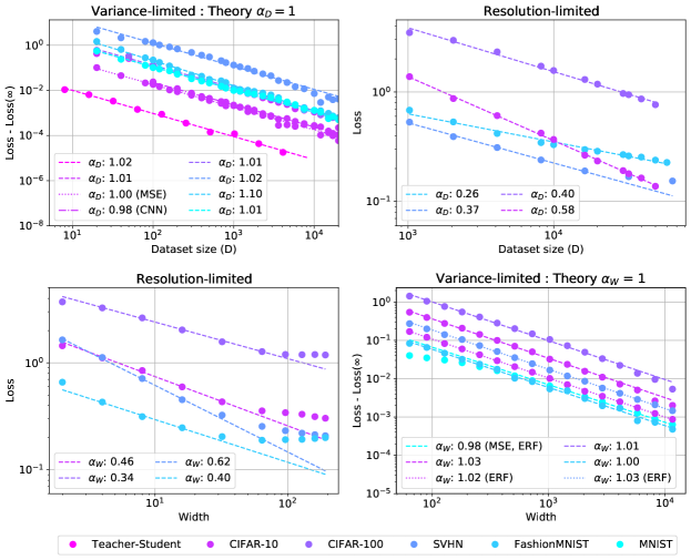
Figure 1: Four scaling regimes Here we exhibit the four regimes we focus on in this work. (top-left, bottom-right) Variance-limited scaling of under-parameterized models with dataset size and over-parameterized models with number of parameters (width) exhibit universal scaling ($\alpha_{D}=\alpha_{W}=1$) independent of the architecture or underlying dataset. (top-right, bottom-left) Resolution-limited over-parameterized models with dataset or under-parameterized models with model size exhibit scaling with exponents that depend on the details of the data distribution. These four regimes are also found in random feature (Figure 3) and pretrained models (see supplement).

1 Scaling Laws for Neural Networks

For a large variety of models and datasets, neural network performance has been empirically observed to scale as a power-law with model size and dataset size [1, 2, 3, 4]. We would like to understand why these power laws emerge, and what features of the data and models determine the values of the power-law exponents. Since these exponents determine how quickly performance improves with more data and larger models, they are of great importance when considering whether to scale up existing models.

In this work, we present a theoretical framework for explaining scaling laws in trained neural networks. We identify four related scaling regimes with respect to the number of model parameters $P$ and the dataset size $D$. With respect to each of $D$, $P$, there is both a resolution-limited regime and a variance-limited regime.

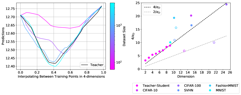
Figure 2: Resolution-limited models interpolate the data manifold Linear interpolation between two training points in a four-dimensional input space (left). We show a teacher model and four student models, each trained on different sized datasets. In all cases teacher and student approximately agree on the training endpoints, but as the training set size increases they increasingly match everywhere. (right) We show $4/\alpha_{D}$ versus the data manifold dimension (input dimension for teacher-student models, intrinsic dimension for standard datasets). We find that the teacher-student models follow the $4/\alpha_{D}$ (dark dashed line), while the relationship for a four layer CNN (solid) and WRN (hollow) on standard datasets is less clear.

Variance-Limited Regime

In the limit of infinite data or an arbitrarily wide model, some aspects of neural network training simplify. Specifically, if we fix one of $D,P$ and study scaling with respect to the other parameter as it becomes arbitrarily large, then the loss scales as $1/x$, i.e. as a power-law with exponent $1$, with $x=D$ or $\sqrt{P}\propto$ width in deep networks and $x=D$ or $P$ in linear models. In essence, this variance-limited regime is amenable to analysis because model predictions can be series expanded in either inverse width or inverse dataset size. To demonstrate these variance-limited scalings, it is sufficient to argue that the infinite data or width limit exists and is smooth; this guarantees that an expansion in simple integer powers exists.

Resolution-Limited Regime

In this regime, one of $D$ or $P$ is effectively infinite, and we study scaling as the other parameter increases. In this case, a variety of works have empirically observed power-law scalings $1/x^{\alpha}$, typically with $0<\alpha<1$ for both $x=P$ or $D$.

We can provide a very general argument for power-law scalings if we assume that trained models map the data into a $d$-dimensional data manifold. The key idea is then that additional data (in the infinite model-size limit) or added model parameters (in the infinite data limit) are used by the model to carve up the data manifold into smaller components. The model then makes independent predictions in each component of the data manifold in order to optimize the training loss.

If the underlying data varies continuously on the manifold, then the size of the sub-regions into which we can divide the manifold (rather than the number of regions) determines the model’s loss. To shrink the size of the sub-regions by a factor of 2 requires increasing the parameter count or dataset size by a factor of $2^{d}$, and so the inverse of the scaling exponent will be proportional to the intrinsic dimension $d$ of the data manifold, so that $\alpha\propto 1/d$. A visualization of this successively better approximation with dataset size is shown in Figure 2 for models trained to predict data generated by a random fully-connected network.

Explicit Realization

These regimes can be realized in linear models, and this includes linearized versions of neural networks via the large width limit. In these limits, we can solve for the test error directly in terms of the feature covariance (kernel). The scaling of the test loss then follows from the asymptotic decay of the spectrum of the covariance matrix. Furthermore, well-known theorems provide bounds on the spectra associated with continuous kernels on a $d$-dimensional manifold. Since otherwise generic kernels saturate these bounds, we find a tight connection between the dimension of the data manifold, kernel spectra, and scaling laws for the test loss. We emphasize, this analysis relies on an implicit model of realistic data only through the assumption of a generic, power law kernel spectrum.

Summary of Contributions:

1. We identify four scaling regions of neural networks and provide empirical support for all four regions for deep models on standard datasets. To our knowledge, the variance-limited dataset scaling has not been exhibited previously for deep networks on realistic data.

2. We present simple yet general theoretical assumptions under which we can derive this scaling behavior. In particular, we relate the scaling exponent in the resolution-limited regime to the intrinsic dimension of the data-manifold realized by trained networks representations.

3. We present a concrete solvable example where all four scaling behaviors can be observed and understood: linear, random-feature teacher-student models.

4. We empirically investigate the dependence of the scaling exponent on changes in architecture and data. We find that changing the input distribution via switching datasets, or the addition of noise has a strong effect on the exponent, while changing the target distribution via superclassing does not.

1.1 Related Works

There have been a number of recent works demonstrating empirical scaling laws [hestness2017deep, kaplan2020scaling, rosenfeld2020a, henighan2020scaling, rosenfeld2020predictability] in deep neural networks, including scaling laws with model size, dataset size, compute, and other observables such as mutual information and pruning. Some precursors [ahmad1989scaling, cohn1991] can be found in earlier literature.

There has been comparatively little work on theoretical ideas [sharma2020neural] that match and explain empirical findings in generic deep neural networks across a range of settings. In the particular case of large width, deep neural networks behave as random feature models [nealthesis, lee2018deep, matthews2018, Jacot2018ntk, lee2019wide, Dyer2020Asymptotics], and known results on the loss scaling of kernel methods can be applied [spigler2020asymptotic, bordelon2020spectrum]. During the completion of this work [hutter2021learning] presented a solvable model of learning exhibiting non-trivial power-law scaling for power-law (Zipf) distributed features.

In the variance-limited regime, scaling laws in the context of random feature models [rahimi2008weighted, hastie2019surprises, d2020double], deep linear models [advani2017high, advani2020high], one-hidden-layer networks [mei2019generalization, adlam2020neural, adlam2020understanding], and wide neural networks treated as Gaussian processes or trained in the NTK regime [lee2019wide, Dyer2020Asymptotics, andreassen2020, geiger2020scaling] have been studied. In particular, this behavior was used in [kaplan2020scaling] to motivate a particular ansatz for simultaneous scaling with data and model size.

This work also makes use of classic results connecting the spectrum of a smooth kernel to the geometry it is defined over [weyl1912asymptotische, reade1983eigenvalues, kuhn1987eigenvalues, ferreira2009eigenvalues] and on the scaling of iteratively refined approximations to smooth manifolds [stein1999interpolation, bickel2007local, de2011approximating].

Recently, scaling laws have also played a significant role in motivating work on the largest models that have yet been developed [brown2020language, fedus2021switch].

2 Theory

Throughout this work we will be interested in how the average test loss $L(D,P)$ depends on the dataset size $D$ and the number of model parameters $P$. Unless otherwise noted, $L$ denotes the test loss averaged over model initializations and draws of a size $D$ training set. Some of our results only pertain directly to the scaling with width $w\propto\sqrt{P}$, but we expect many of the intuitions apply more generally. We use the notation $\alpha_{D}$, $\alpha_{P}$, and $\alpha_{W}$ to indicate scaling exponents with respect to dataset size, parameter count, and width.

2.1 Variance-Limited Exponents

In the limit of large $D$ the outputs of an appropriately trained network approach a limiting form with corrections which scale as $D^{-1}$. Similarly, recent work shows that wide networks have a smooth large $P$ limit, [Jacot2018ntk], where fluctuations scale as $1/\sqrt{P}$. If the loss is analytic about this limiting model then its value will approach the asymptotic loss with corrections proportional to the variance, ($1/D$ or $1/\sqrt{P}$). Let us discuss this in a bit more detail for both cases.

2.1.1 Dataset scaling

Consider a neural network, and its associated training loss $L_{\textrm{train}}(\theta)$. For every value of the weights, the training loss, thought of as a random variable over draws of a training set of size $D$, concentrates around the population loss, with a variance which scales as $\mathcal{O}\left(D^{-1}\right)$. Thus, if the optimization procedure is sufficiently smooth, the trained weights, network output, and test loss will approach their infinite $D$ values plus an $\mathcal{O}\left(D^{-1}\right)$ contribution.

As a concrete example, consider training a network via full-batch optimization. In the limit that $D\to\infty$, the gradients will become exactly equal to the gradient of the population loss. When $D$ is large but finite, the gradient will include a term proportional to the $\mathcal{O}(D^{-1})$ variance of the loss over the dataset. This means that the final parameters will be equal to the parameters from the $D\rightarrow\infty$ limit of training plus some term proportional to $D^{-1}$. This also carries over to the test loss.

Since this argument applies to any specific initialization of the parameters, it also applies when we take the expectation of the test loss over the distribution of initializations. We do not prove the result rigorously at finite batch size. We expect it to hold however, in expectation over instances of stochastic optimization, provided hyper-parameters (such as batch size) are fixed as $D$ is taken large.

2.1.2 Large Width Scaling

We can make a very similar argument in the $w\to\infty$ or large width limit. It has been shown that the predictions from an infinitely wide network, either at initialization [nealthesis, lee2018deep], or when trained via gradient descent [Jacot2018ntk, lee2019wide] approach a limiting distribution equivalent to training a linear model. Furthermore, corrections to the infinite width behavior are controlled by the variance of the full model around the linear model predictions. This variance has been shown to scale as $1/w$ [Dyer2020Asymptotics, yaida2019non, andreassen2020]. As the loss is a smooth function of these predictions, it will differ from its $w=\infty$ limit by a term proportional to $1/w$.

We note that there has also been work studying the combined large depth and large width limit, where Hanin2020Finite found a well-defined infinite size limit with controlled fluctuations. In any such context where the model predictions concentrate, we expect the loss to scale with the variance of the model output. In the case of linear models, studied below, the variance is $\mathcal{O}(P^{-1})$ rather than $\mathcal{O}(\sqrt{P})$ and we see the associated variance scaling in this case.

2.2 Resolution-Limited Exponents

In this section we consider training and test data drawn uniformly from a compact $d$-dimensional manifold, $x\in\mathcal{M}_{d}$ and targets given by some smooth function $y=\mathcal{F}(x)$ on this manifold.

2.2.1 Over-parameterized dataset scaling

Consider the double limit of an over-parameterized model with large training set size, $P\gg D\gg 1$. We further consider well trained models, i.e. models that interpolate all training data. The goal is to understand $L(D)$. If we assume that the learned model $f$ is sufficiently smooth, then the dependence of the loss on $D$ can be bounded in terms of the dimension of the data manifold $\mathcal{M}_{d}$.

Informally, if our train and test data are drawn i.i.d. from the same manifold, then the distance from a test point to the closest training data point decreases as we add more and more training data points. In particular, this distance scales as $\mathcal{O}(D^{-1/d})$ [levina2005maximum]. Furthermore, if $f$, $\mathcal{F}$ are both sufficiently smooth, they cannot differ too much over this distance. If in addition the loss function, $L$, is a smooth function vanishing when $f=\mathcal{F}$, we have $L=\mathcal{O}(D^{-1/d})$. This is summarized in the following theorem.

Theorem 1.

Let $L(f)$, $f$ and $\mathcal{F}$ be Lipschitz with constants $K_{L}$, $K_{f}$, and $K_{\mathcal{F}}$. Further let $\mathcal{D}$ be a training dataset of size $D$ sampled i.i.d from $\mathcal{M}_{d}$ and let $f(x)=\mathcal{F}(x),\,\,\forall x\in\mathcal{D}$ then $L(D)=\mathcal{O}\left(K_{L}\textrm{max}{(K_{f},K_{\mathcal{F}})}D^{-1/d}\right)$.

2.2.2 Under-Parameterized Parameter Scaling

We will again assume that $\mathcal{F}$ varies smoothly on an underlying compact $d$-dimensional manifold $\mathcal{M}_{d}$. We can obtain a bound on $L(P)$ if we imagine that $f$ approximates $\mathcal{F}$ as a piecewise linear function with roughly $P$ regions (see sharma2020neural). Here, we instead make use of the argument from the over-parameterized, resolution-limited regime above. If we construct a sufficiently smooth estimator for $\mathcal{F}$ by interpolating among $P$ randomly chosen points from the (arbitrarily large) training set, then by the argument above the loss will be bounded by $\mathcal{O}(P^{-1/d})$.

Theorem 2.

Let $L(f)$, $f$ and $\mathcal{F}$ be Lipschitz with constants $K_{L}$, $K_{f}$, and $K_{\mathcal{F}}$. Further let $f(x)=\mathcal{F}(x)$ for $P$ points sampled i.i.d from $\mathcal{M}_{d}$ then $L(P)=\mathcal{O}\left(K_{L}\textrm{max}{(K_{f},K_{\mathcal{F}})}P^{-1/d}\right)$.

We provide the proof of Theorem 1 and 2 in the supplement.

2.2.3 From Bounds to Estimates

Theorems 1 and 2 are phrased as bounds, but we expect the stronger statement that these bounds also generically serve as estimates, so that eg $L(D)=\Omega(D^{-c/d})$ for $c\geq 2$, and similarly for parameter scaling. If we assume that $\mathcal{F}$ and $f$ are analytic functions on $\mathcal{M}_{d}$ and that the loss function $L(f,\mathcal{F})$ is analytic in $f-\mathcal{F}$ and minimized at $f=\mathcal{F}$, then the loss at a given test input, $x_{\textrm{test}}$, can be expanded around the nearest training point, $\hat{x}_{\textrm{train}}$.

$$\begin{split}L(x_{\textrm{test}})&=\sum_{m=n\geq 2}^{\infty}a_{m}(\hat{x}_{\textrm{train}})(x_{\textrm{test}}-\hat{x}_{\textrm{train}})^{m}\,,\end{split}$$ (1)

where the first term is of finite order $n\geq 2$ because the loss vanishes at the training point. As the typical distance between nearest neighbor points scales as $D^{-1/d}$ on a $d$-dimensional manifold, the loss will be dominated by the leading term, $L\propto D^{-n/d}$, at large $D$. Note that if the model provides an accurate piecewise linear approximation, we will generically find $n\geq 4$.

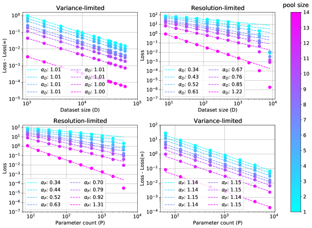
Figure 3: Random feature models exhibit all four scaling regimes Here we consider linear teacher-student models with random features trained with MSE loss to convergence. We see both variance-limited scaling (top-left, bottom-right) and resolution-limited scaling (top-right, bottom-left). Data is varied by downsampling MNIST by the specified pool size.

2.3 Kernel realization

In the proceeding sections we have conjectured typical case scaling relations for a model’s test loss. We have further given intuitive arguments for this behavior which relied on smoothness assumptions about the loss and training procedure. In this section, we provide a concrete realization of all four scaling regimes within the context of linear models. Of particular interest is the resolution-limited regime, where the scaling of the loss is a consequence of the linear model kernel spectrum – the scaling of over-parameterized models with dataset size and under-parameterized models with parameters is a consequence of a classic result, originally due to weyl1912asymptotische, bounding the spectrum of sufficiently smooth kernel functions by the dimension of the manifold they act on.

Linear predictors serve as a model system for learning. Such models are used frequently in practice when more expressive models are unnecessary or infeasible [mccullagh1989generalized, rifkin2007notes, hastie2009elements] and also serve as an instructive test bed to study training dynamics [advani2020high, goh2017why, hastie2019surprises, nakkiran2019more, grosse-notes]. Furthermore, in the large width limit, randomly initialized neural networks become Gaussian Processes [nealthesis, lee2018deep, matthews2018, novak2018bayesian, garriga2018deep, yang2019scaling], and in the low-learning rate regime [lee2019wide, lewkowycz2020large, huang_largelr] neural networks train as linear models at infinite width [Jacot2018ntk, lee2019wide, chizat2019lazy].

Here we discuss linear models in general terms, though the results immediately hold for the special cases of wide neural networks. In this section we focus on teacher-student models with weights initialized to zero and trained with mean squared error (MSE) loss to their global optimum.

We consider a linear teacher, $F$, and student $f$.

$$\begin{split}F(x)=\sum_{M=1}^{S}\omega_{M}F_{M}(x),\ \ \ f(x)&=\sum_{\mu=1}^{P}\theta_{\mu}f_{\mu}(x)\,.\end{split}$$ (2)

Here $\{F_{M}\}$ are a (potentially infinite) pool of features and the teacher weights, $\omega_{M}$ are taken to be normal distributed, $\omega\sim\mathcal{N}(0,1/S)$.

The student model is built out of a subset of the teacher features. To vary the number of parameters in this simple model, we construct $P$ features, $f_{\mu=1,\ldots,P}$, by introducing a projector $\mathcal{P}$ onto a $P$-dimensional subspace of the teacher features, $f_{\mu}=\sum_{M}\mathcal{P}_{\mu M}F_{M}$.

We train this model by sampling a training set of size $D$ and minimizing the MSE training loss,

$$\begin{split}L_{\textrm{train}}&=\frac{1}{2D}\sum_{a=1}^{D}\left(f(x_{a})-F(x_{a})\right)^{2}\,.\end{split}$$ (3)

We are interested in the test loss averaged over draws of our teacher and training dataset. In the limit of infinite data, the test loss, $L(P):=\lim_{D\rightarrow\infty}L(D,P)$, takes the form.

$$\begin{split}L(P)&=\frac{1}{2S}\textrm{Tr}\left[\mathcal{C}-\mathcal{C}\mathcal{P}^{T}\left(\mathcal{P}\mathcal{C}\mathcal{P}^{T}\right)^{-1}\mathcal{P}\mathcal{C}\right]\,.\end{split}$$ (4)

Here we have introduced the feature-feature second moment-matrix, $\mathcal{C}=\mathbb{E}_{x}\left[F(x)F^{T}(x)\right]$.

If the teacher and student features had the same span, this would vanish, but as a result of the mismatch the loss is non-zero. On the other hand, if we keep a finite number of training points, but allow the student to use all of the teacher features, the test loss, $L(D):=\lim_{P\rightarrow S}L(D,P)$, takes the form,

$$\begin{split}L(D)=\frac{1}{2}\mathbb{E}_{x}\left[\mathcal{K}(x,x)-\vec{\mathcal{K}}(x)\bar{\mathcal{K}}^{-1}\vec{\mathcal{K}}(x)\right]\,.\end{split}$$ (5)

Here, $\mathcal{K}(x,x^{\prime})$ is the data-data second moment matrix, $\vec{\mathcal{K}}$ indicates restricting one argument to the $D$ training points, while $\bar{\mathcal{K}}$ indicates restricting both. This test loss vanishes as the number of training points becomes infinite but is non-zero for finite training size.

We present a full derivation of these expressions in the supplement. In the remainder of this section, we explore the scaling of the test loss with dataset and model size.

2.3.1 Kernels: Variance-Limited exponents

To derive the limiting expressions (4) and (5) for the loss one makes use of the fact that the sample expectation of the second moment matrix over the finite dataset, and finite feature set is close to the full covariance.

$$\begin{split}\frac{1}{D}\sum_{a=1}^{D}F(x_{a})F^{T}(x_{a})\,=\,\mathcal{C}+\delta\mathcal{C}\,,\ \ \ \frac{1}{P}f^{T}(x)f(x^{\prime}),=\,\mathcal{K}+\delta\mathcal{K}\,,\end{split}$$

with the fluctuations satisfying $\mathbb{E}_{D}\left[\delta C^{2}\right]=\mathcal{O}(D^{-1})$ and $\mathbb{E}_{P}\left[\delta K^{2}\right]=\mathcal{O}(P^{-1})$, where expectations are taken over draws of a dataset of size $D$ and over feature sets.

Using these expansions yields the variance-limited scaling, $L(D,P)-L(P)=\mathcal{O}(D^{-1})$, $L(D,P)-L(D)=\mathcal{O}(P^{-1})$ in the under-parameterized and over-parameterized settings respectively.

In Figure 3 we see evidence of these scaling relations for features built from randomly initialized ReLU networks on pooled MNIST independent of the pool size. In the supplement we provide an in depth derivation of this behavior and expressions for the leading contributions to $L(D,P)-L(P)$ and $L(D,P)-L(D)$.

2.3.2 Kernels: Resolution-limited exponents

We now would like to analyze the scaling behavior of our linear model in the resolution-limited regimes, that is the scaling with $P$ when $1\ll P\ll D$ and the scaling with $D$ when $1\ll D\ll P$. In these cases, the scaling is controlled by the shared spectrum of $\mathcal{C}$ or $\mathcal{K}$. This spectrum is often well described by a power-law, where eigenvalues $\lambda_{i}$ satisfy

$$\begin{split}\lambda_{i}&=\frac{1}{i^{1+\alpha_{K}}}\,.\end{split}$$ (6)

See Figure 4 for example spectra on pooled MNIST.

In this case, we will argue that the losses also obey a power law scaling, with the exponents controlled by the spectral decay factor, $1+\alpha_{K}$.

$$\begin{split}L(D)\propto D^{-\alpha_{K}}\,,\ \ \ L(P)\propto P^{-\alpha_{K}}\,.\end{split}$$ (7)

In other words, in this setting, $\alpha_{P}=\alpha_{D}=\alpha_{K}$.

This is supported empirically in Figure 4. We then argue that when the kernel function, $\mathcal{K}$ is sufficiently smooth on a manifold of dimension $d$, $\alpha_{K}\propto d^{-1}$, thus realizing the more general resolution-limited picture described above.

From spectra to scaling laws for the loss

To be concrete let us focus on the over-parameterized loss. If we introduce the notation $e_{i}$ for the eigenvectors of $\mathcal{C}$ and $\bar{e}_{i}$ for the eignvectors of $\frac{1}{D}\sum_{a=1}^{D}F(x_{a})F^{T}(x_{a})$, the loss becomes,

$$\begin{split}L(D)=\frac{1}{2}\sum_{i=1}^{S}\lambda_{i}(1-\sum_{j=1}^{D}(e_{i}\cdot\bar{e}_{j})^{2})\,.\end{split}$$ (8)

Before discussing the general asymptotic behavior of (8), we can gain some intuition by considering the case of large $\alpha_{K}$. In this case, $\bar{e}_{j}\approx e_{j}$ (see e.g. loukas2017close), we can simplify (8) to,

$$\begin{split}L(D)&\propto\sum_{D+1}^{\infty}\frac{1}{i^{1+\alpha_{K}}}=\alpha_{K}D^{-\alpha_{K}}+\mathcal{O}(D^{-\alpha_{K}-1})\,.\end{split}$$ (9)

More generally in the supplement, following bordelon2020spectrum, canatar2020statistical, we use replica theory methods to derive, $L(D)\propto D^{-\alpha_{K}}$ and $L(P)\propto P^{-\alpha_{K}}$, without requiring the large $\alpha_{K}$ limit.

Data Manifolds and Kernels

In Section 2.2, we discussed a simple argument that resolution-limited exponents $\alpha\propto 1/d$, where $d$ is the dimension of the data manifold. Our goal now is to explain how this connects with the linearized models and kernels discussed above: how does the spectrum of eigenvalues of a kernel relate to the dimension of the data manifold?

The key point is that sufficiently smooth kernels must have an eigenvalue spectrum with a bounded tail. Specifically, a $C^{t}$ kernel on a $d$-dimensional space must have eigenvalues $\lambda_{n}\lesssim\frac{1}{n^{1+t/d}}$ [kuhn1987eigenvalues]. In the generic case where the covariance matrices we have discussed can be interpreted as kernels on a manifold, and they have spectra saturating the bound, linearized models will inherit scaling exponents given by the dimension of the manifold.

As a simple example, consider a $d$-torus. In this case we can study the Fourier series decomposition, and examine the case of a kernel $K(x-y)$. This must take the form

$$K=\sum_{n_{I}}\left[a_{n_{I}}\sin(n_{I}\cdot(x-y))+b_{n_{I}}\cos(n_{I}\cdot(x-y))\right]$$

where $n_{I}=(n_{1},\cdots,n_{d})$ is a list of integer indices, and $a_{n_{I}}$, $b_{n_{I}}$ are the overall Fourier coefficients. To guarantee that $K$ is a $C^{t}$ function, we must have $a_{n_{I}},b_{n_{I}}\lesssim\frac{1}{n^{d+t}}$ where $n^{d}=N$ indexes the number of $a_{n_{I}}$ in decreasing order. But this means that in this simple case, the tail eigenvalues of the kernel must be bounded by $\frac{1}{N^{1+t/d}}$ as $N\to\infty$.

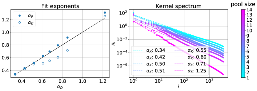
Figure 4: Duality and spectra in random feature models Here we show the relation between the decay of the kernel spectra, $\alpha_{K}$, and the scaling of the loss with number of data points, $\alpha_{D}$, and with number of parameters, $\alpha_{P}$ (left). The theoretical relation $\alpha_{D}=\alpha_{P}=\alpha_{K}$ is given by the black dashed line. (right) The spectra of random FC kernels on pooled MNIST. The spectra appear well described by a power law decay.

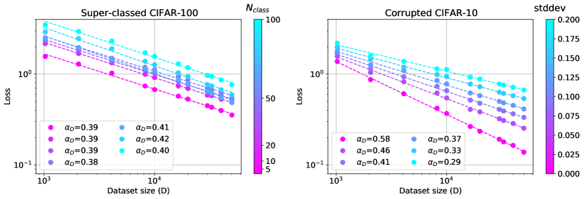
Figure 5: Effect of data distribution on scaling exponents For CIFAR-100 superclassed to $N$ classes (left), we find that the number of target classes does not have a visible effect on the scaling exponent. (right) For CIFAR-10 with the addition of Gaussian noise to inputs, we find the strength of the noise has a strong effect on performance scaling with dataset size. All models are WRN-28-10.

2.4 Duality

We argued above that for kernels with pure power law spectra, the asymptotic scaling of the under-parameterized loss with respect to model size and the over-parameterized loss with respect to dataset size share a common exponent. In the linear setup at hand, the relation between the under-parameterized parameter dependence and over-parameterized dataset dependence is even stronger. The under-parameterized and over-parameterized losses are directly related by exchanging the projection onto random features with the projection onto random training points. Note, sample-wise double descent observed in nakkiran2019more is a concrete realization of this duality for a simple data distribution. In the supplement, we present examples exhibiting the duality of the loss dependence on model and dataset size outside of the asymptotic regime.

3 Experiments

3.1 Deep teacher-student models

Our theory can be tested very directly in the teacher-student framework, in which a teacher deep neural network generates synthetic data used to train a student network. Here, it is possible to generate unlimited training samples and, crucially, controllably tune the dimension of the data manifold. We accomplish the latter by scanning over the dimension of the inputs to the teacher. We have found that when scanning over both model size and dataset size, the interpolation exponents closely match the prediction of $4/d$. The dataset size scaling is shown in Figure 2, while model size scaling experiments appear in the supplement and have previously been observed in sharma2020neural.

3.2 Variance-limited scaling in the wild

Variance-limited scaling can be universally observed in real datasets. The theory describing the variance scaling in Section 2.1 does not make any particular assumptions about data, model or loss type, beyond smoothness. Figure 1 (top-left, bottom-right) measures the variance-limited dataset scaling exponent $\alpha_{D}$ and width scaling exponent $\alpha_{W}$. In both cases, we find striking agreement with the theoretically predicted values $\alpha_{D},\alpha_{W}=1$ across a variety of dataset, network architecture, and loss type combinations.

Our testbed includes deep fully-connected and convolutional networks with Relu or Erf nonlinearities and MSE or softmax-cross-entropy losses. Experiments in Figure 1 (top-left) utilize relatively small models, with the number of trainable parameteters $P\sim\mathcal{O}(1000)$, trained with full-batch gradient descent (GD) and small learning rate on datasets of size $D\gg P$. Each data point in the figure represents an average over subsets of size $D$ sampled from the full dataset. Conversely, experiments in Figure 1 (bottom-right) utilize a small, fixed dataset $D\sim\mathcal{O}(100)$, trained with full-batch GD and small learning rate using deep networks with widths $w\gg D$. As detailed in the supplement, each data point is an average over random initializations, where the infinite-width contribution to the loss has been computed and subtracted off prior to averaging.

3.3 Resolution-limited scaling in the wild

In addition to teacher-student models, we explored resolution-limited scaling behavior in the context of standard classification datasets. Experiments were performed with the Wide ResNet (WRN) architecture [zagoruyko2016wide] and trained with cosine decay for a number of steps equal to 200 epochs on the full dataset. In Figure 2 we also include data from a four hidden layer CNN detailed in the supplement. As detailed above, we find dataset dependent scaling behavior in this context.

We further investigated the effect of the data distribution on the resolution-limited exponent, $\alpha_{D}$ by tuning the number of target classes and input noise (Figure 5).

To probe the effect of the number of target classes, we constructed tasks derived from CIFAR-100 by grouping classes into broader semantic categories. We found that performance depends on the number of categories, but $\alpha_{D}$ is insensitive to this number. In contrast, the addition of Gaussian noise had a more pronounced effect on $\alpha_{D}$. These results suggest a picture in which the network learns to model the input data manifold, independent of the classification task, consistent with observations in nakkiran2020distributional, Grathwohl2020Your.

We also explored the effect of network aspect ratio on the dataset scaling exponent. We found that the exponent magnitude increases with width up to a critical width, while the dependence on depth is more mild (see the supplement).

4 Discussion

We have presented a framework for categorizing neural scaling laws, along with derivations that help to explain their very general origins. Crucially, our predictions agree with empirical findings in settings which have often proven challenging for theory – deep neural networks on real datasets.

The variance-scaling regime yields, for smooth test losses, a universal prediction of $\alpha_{D}=1$ (for $D\gg P$) and $\alpha_{W}=1$ (for $w\gg D$). The resolution-limited regime – more closely tied to the regime in which real neural networks are trained in practice – yields exponents $\alpha_{D},\alpha_{P}$ whose numerical value is variable, but we have traced their origins back to a single simple quantity: the intrinsic dimension of the data manifold $d$, which in a general setting is significantly smaller than the input dimension. In linear models, this is also closely related to $\alpha_{K}$, the exponent governing the power-law spectral decay of certain kernels. Neural scaling laws depend on the data distribution, but perhaps they only depend on ‘macroscopic’ properties such as spectra or a notion of intrinsic dimensionality.

Along the way, our empirical investigations have revealed some additional intriguing observations. The invariance of the dataset scaling exponent to superclassing (Figure 5) suggests that commonly-used deep networks may be largely learning properties of the input data manifold – akin to unsupervised learning – rather than significant task-specific structure, which may shed light on the versatility of learned deep network representations for different downstream tasks.

In our experiments, models with larger exponents do indeed tend to perform better, due to increased sample or model efficiency. We see this in the teacher-student setting for models trained on real datasets and in the supplement find that trained features scale noticeably better than random features. This suggests the scaling exponents and intrinsic dimension as possible targets for meta-learning and neural architecture search.

On a broader level, we think work on neural scaling laws provides an opportunity for discussion in the community on how to define and measure progress in machine learning. The values of the exponents allow us to concretely estimate expected gains that come from increases in scale of dataset, model, and compute, albeit with orders of magnitude more scale for constant-factor improvements. On the other hand, one may require that truly non-trivial progress in machine learning be progress that occurs modulo scale: namely, improvements in performance across different tasks that are not simple extrapolations of existing behavior. And perhaps the right combinations of algorithmic, model, and dataset improvements can lead to emergent behavior at new scales. Large language models such as GPT-3 (Fig. 1.2 in [brown2020language]) have exhibited this in the context of few-shot learning. We hope our work spurs further research in understanding and controlling neural scaling laws.

Supplemental Material

Appendix A Experimental setup

Figure 1 (top-left) Experiments are done using Neural Tangents [neuraltangents2020] based on JAX [jaxrepro]. All experiment except denoted as (CNN), use 3-layer, width-8 fully-connected networks. CNN architecture used is Myrtle-5 network [Shankar2020NeuralKW] with 8 channels. Relu activation function with critical initialization [schoenholz2016deep, lee2018deep, xiao18a] was used. Unless specified softmax-cross-entropy loss was used. We performed full-batch gradient descent update for all dataset sizes without L2 regularization. 20 different training data sampling seed was averaged for each point. For fully-connected network input pooling of size 4 was performed for CIFAR-10/100 dataset and pooling of size 2 was performed for MNIST and Fashion-MNIST dataset. This was to reduce number of parameters in the input layer (# of pixels $\times$ width) which can be quite large even for small width networks.

Figure 1 (top-right) All experiments were performed using a Flax [flax2020github] implementation of Wide ResNet 28-10 [zagoruyko2016wide], and performed using the Caliban experiment manager [Ritchie2020]. Models were trained for 78125 total steps with a cosine learning rate decay [loshchilov2016sgdr] and an augmentation policy consisting of random flips and crops. We report final loss, though we found no qualitative difference between using final loss, best loss, final accuracy or best accuracy (see Figure S1).

Figure 1 (bottom-left) The setup was identical to Figure 1 (top-right) except that the model considered was a depth 10 residual network with varying width.

Figure 1 (bottom-right) Experiments are done using Neural Tangents. All experiments use 100 training samples and two-hidden layer fully-connected networks of varying width (ranging from $w=64$ to $W=11,585$) with Relu nonlinearities unless specified as Erf. Full-batch gradient descent and cross-entropy loss were used unless specified as MSE, and the figure shows curves from a random assortment of training times ranging from 100 to 500 steps (equivalently, epochs). Training was done with learning rates small enough so as to avoid catapult dynamics [lewkowycz2020large] and no $L2$ regularization; in such a setting, the infinite-width learning dynamics is known to be equivalent to that of linearized models [lee2019wide]. Consequently, for each random initialization of the parameters, the test loss of the finite-width linearized model was additionally computed in the identical training setting. This value approximates the limiting behavior $L(\infty)$ known theoretically and is subtracted off from the final test loss of the (nonlinear) neural network before averaging over 50 random initializations to yield each of the individual data points in the figure.

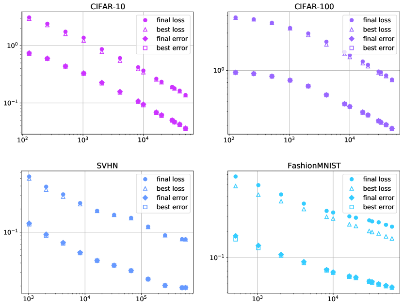
Figure S1: Alternate metrics and stopping conditions We find similar scaling behavior for both the loss and error, and for final and best (early stopped) metrics.

A.1 Deep teacher-student models

The teacher-student scaling with dataset size (figure S2) was performed with fully-connected teacher and student networks with two hidden layers and widths 96 and 192, respectively, using PyTorch [paszke2019pytorch]. The inputs were random vectors sampled uniformly from a hypercube of dimension $d=2,3,\cdots,9$. To mitigate noise, we ran the experiment on eight different random seeds, fixing the random seed for the teacher and student as we scanned over dataset sizes. We also used a fixed test dataset, and a fixed training set, which was sub-sampled for the experiments with smaller $D$. The student networks were trained using MSE loss and Adam optimizer with a maximum learning rate of $3\times 10^{-3}$, a cosine learning rate decay, and a batch size of $64$, and $40,000$ steps of training. The test losses were measured with early stopping. We combine test losses from different random seeds by averaging the logarithm of the loss from each seed.

In our experiments, we always use inputs that are uniformly sampled from a $d$-dimensional hypercube, following the setup of sharma2020neural. They also utilized several intrisic dimension (ID) estimation methods and found the estimates were close to the input dimension, so we simply use the latter for comparisons. For the dataset size scans we used randomly initialized teachers with width 96, and students with width 192. We found similar results with other network sizes.

The final scaling exponents and input dimensions are show in the bottom of figure 2. We used the same experiments for the top of that figure, interpolating the behavior of both teacher and a set of students between two fixed training points. The students only differed by the size of their training sets, but had the same random seeds and were trained in the same way. In that figure the input space dimension was four.

Finally, we also used a similar setup to study variance-limited exponents and scaling. In that case we used much smaller models, with 16-dimensional hidden layers, and a correspondingly larger learning rate. We then studied scaling with $D$ again, with results pictured in figure 1.

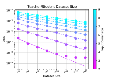
Figure S2: This figure shows scaling trends of MSE loss with dataset size for teacher/student models. The exponents extracted from these fits and their associated input-space dimensionalities are shown in figure 2.

A.2 CNN architecture for resolution-limited scaling

Figure 2 includes data from CNN architectures trained on image datasets. The architectures are summarized in Table 1. We used Adam optimizer for training, with cross-entropy loss. Each network was trained for long enough to achieve either a clear minimum or a plateau in test loss. Specifically, CIFAR10, MNIST and fashion MNIST were trained for $50$ epochs, CIFAR100 was trained for $100$ epochs and SVHN was trained for $10$ epochs. The default keras training parameters were used. In case of SVHN we included the additional images as training data. We averaged (in log space) over $20$ runs for CIFAR100 and CIFAR10, $16$ runs for MNIST, $12$ runs for fashion MNIST, and $5$ runs for SVHN. The results of these experiments are shown in figure S3.

The measurement of input-space dimensionality for these experiemnts was done using the nearest-neighbour algorithm, described in detail in appendix B and C in [sharma2020neural]. We used 2, 3 and 4 nearest neighbors and averaged over the three.

A.3 Teacher-student experiment for scaling of loss with model size

We replicated the teacher-student setup in [sharma2020neural] to demonstrate the scaling of loss with model size. The resulting variation of $-4/\alpha_{P}$ with input-space dimensionality is shown in figure S4. In our implementation we averaged (in log space) over $15$ iterations, with a fixed, randomly generated teacher.

Layer	Width
CNN window (3, 3)	50
2D Max Pooling (2, 2)
CNN window (3, 3)	100
2D Max Pooling (2, 2)
CNN window (3, 3)	100
Dense	64
Dense	10

Layer	Width
CNN window (3, 3)	50
2D Max Pooling (2, 2)
CNN window (3,3)	100
2D Max Pooling (2, 2)
CNN window (3, 3)	200
Dense	256
Dense	100

Layer	Width
CNN window (3, 3)	64
2D Max Pooling (2, 2)
CNN window (3, 3)	64
2D Max Pooling (2, 2)
Dense	128
Dense	10

Table 1: CNN architectures for CIFAR10, MNIST, Fashion MNIST (left), CIFAR100 (center) and SVHN (right)

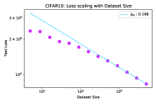
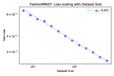
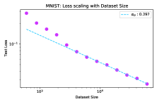
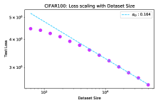
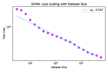
Figure S3: This figure shows scaling trends of CE loss with dataset size for various image datasets. The exponents extracted from these fits and their associated input-space dimensionalities are shown in figure 2.

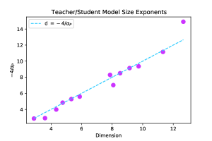
Figure S4: This figure shows the variation of $\alpha_{P}$ with the input-space dimension. The exponent $\alpha_{P}$ is the scaling exponent of loss with model size for Teacher-student setup.

Appendix B Effect of aspect ratio on scaling exponents

We trained Wide ResNet architectures of various widths and depths on CIFAR-10 accross dataset sizes. We found that the effect of depth on dataset scaling was mild for the range studied, while the effect of width impacted the scaling behavior up until a saturating width, after which the scaling behavior fixed. See Figure S5.

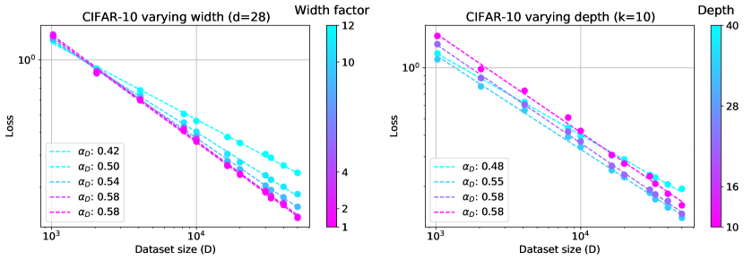
Figure S5: Effect of aspect ratio on dataset scaling We find that for WRN-d-k trained on CIFAR-10, varying depth from 10 to 40 has a relatively mild effect on scaling behavior, while varying the width multiplier, $k$, from 1 to 12 has a more noticeable effect, up until a saturating width.

Appendix C Proof of Theorems 1 and 2

In this section we detail the proof of Theorems 1 and 2. The key observation is to make use of the fact that nearest neighbor distances for $D$ points sampled i.i.d. from a $d$-dimensional manifold have mean $\mathbb{E}_{D,x}\left[\left|x-\hat{x}\right|\right]=\mathcal{O}\left(D^{-1/d}\right)$, where $\hat{x}$ is the nearest neighbor of $x$ and the expectation is the mean over data-points and draws of the dataset see e.g. [levina2005maximum].

The theorem statements are copied for convenience. In the main, in an abuse of notation, we used $L(f)$ to indicate the value of the test loss as a function of the network $f$, and $L(D)$ to indicate the test loss averaged over the population, draws of the dataset, model initializations and training. To be more explicit below, we will use the notation $\ell(f(x))$ to indicate the test loss for a single network evaluated at single test point.

Theorem 1.

Let $\ell(f)$, $f$ and $\mathcal{F}$ be Lipschitz with constants $K_{L}$, $K_{f}$, and $K_{\mathcal{F}}$ and $\ell(\mathcal{F})=0$. Further let $\mathcal{D}$ be a training dataset of size $D$ sampled i.i.d from $\mathcal{M}_{d}$ and let $f(x)=\mathcal{F}(x),\,\,\forall x\in\mathcal{D}$ then $L(D)=\mathcal{O}\left(K_{L}\textrm{max}{(K_{f},K_{\mathcal{F}})}D^{-1/d}\right)$.

Proof.

Consider a network trained on a particular draw of the training data. For each training point, $x$, let $\hat{x}$ denote the neighboring training data point. Then by the above Lipschitz assumptions and the vanishing of the loss on the true target, we have $\ell(f(x))\leq K_{L}\left|f(x)-\mathcal{F}(x)\right|\leq K_{L}\left(K_{f}+K_{\mathcal{F}}\right)\left|x-\hat{x}\right|$. With this, the average test loss is bounded as

$$\begin{split}L(D)\leq K_{L}\left(K_{f}+K_{\mathcal{F}}\right)\mathbb{E}_{D,x}\left[\left|x-\hat{x}\right|\right]=\mathcal{O}\left(K_{L}\textrm{max}{(K_{f},K_{\mathcal{F}})}D^{-1/d}\right)\,.\end{split}$$ (S1)

In the last equality, we used the above mentioned scaling of nearest neighbor distances. ∎

Theorem 2.

Let $\ell(f)$, $f$ and $\mathcal{F}$ be Lipschitz with constants $K_{L}$, $K_{f}$, and $K_{\mathcal{F}}$. Further let $f(x)=\mathcal{F}(x)$ for $P$ points sampled i.i.d from $\mathcal{M}_{d}$ then $L(P)=\mathcal{O}\left(K_{L}\textrm{max}{(K_{f},K_{\mathcal{F}})}P^{-1/d}\right)$.

Proof.

Denote by $\mathcal{P}$ the $P$ points, $z$, for which $f(z)=\mathcal{F}(z)$. For each test point $x$ let $\hat{x}$ denote the closest point in $\mathcal{P}$, $\hat{x}=\textrm{argmin}_{\mathcal{P}}\left(|x-z|\right)$. Adopting this notation, the result follows by the same argument as Theorem 1. ∎

Appendix D Random feature models

Here we present random feature models in more detail. We begin by reviewing exact expressions for the loss. We then go onto derive its asymptotic properties. We again consider training a model $f(x)=\sum_{\mu=1}^{P}\theta_{\mu}f_{\mu}(x)$, where $f_{\mu}$ are drawn from some larger pool of features, $\{F_{M}\}$, $f_{\mu}(x)=\sum_{M=1}^{S}\mathcal{P}_{\mu M}F_{M}(x)$.

Note, if $\{F_{M}(x)\}$ form a complete set of functions over the data distribution, than any target function, $y(x)$, can be expressed as $y=\sum_{M=1}^{S}\omega_{M}F_{M}(x)$. The extra constraint in a teacher-student model is specifying the distribution of the $\omega_{M}$. The variance-limited scaling goes through with or without the teacher-student assumption, however it is crucial for analysing the variance-limited behavior.

As in Section 2.3 we consider models with weights initialized to zero and trained to convergence with mean squared error loss.

$$\begin{split}L_{\textrm{train}}&=\frac{1}{2D}\sum_{a=1}^{D}\left(f(x_{a})-y_{a}\right)^{2}\,.\end{split}$$ (S2)

The data and feature second moments play a central role in our analysis. We introduce the notation,

$$\begin{split}&\mathcal{C}=\mathbb{E}_{x}\left[F(x)F^{T}(x)\right]\,,\ \ \ \bar{\mathcal{C}}=\frac{1}{D}\sum_{a=1}^{D}F(x_{a})F^{T}(x_{a})\,,\ \ \ C=\mathcal{P}\mathcal{C}\mathcal{P}^{T}\,,\ \ \ \bar{C}=\mathcal{P}\bar{\mathcal{C}}\mathcal{P}^{T}\,.\\ &\mathcal{K}(x,x^{\prime})=\frac{1}{S}F^{T}(x)F(x^{\prime})\,,\ \ \ \bar{\mathcal{K}}=\mathcal{K}\Big{|}_{\mathcal{D}_{\textrm{train}}}\,,\ \ \ K(x,x^{\prime})=\frac{1}{P}f^{T}(x)f(x^{\prime})\,,\ \ \ \bar{K}=K\Big{|}_{\mathcal{D}_{\textrm{train}}}\,.\\ \end{split}$$ (S3)

Here the script notation indicates the full feature space while the block letters are restricted to the student features. The bar represents restriction to the training dataset. We will also indicate kernels with one index in the training set as $\vec{\mathcal{K}}(x):=\mathcal{K}(x,x_{a=1\ldots D})$ and $\vec{K}(x):=K(x,x_{a=1\ldots D})$. After this notation spree, the test loss can be written for under-parameterized models, $P\leq D$ as

$$\begin{split}L(D,P)&=\frac{1}{2S}\mathbb{E}_{D}\left[\operatorname{Tr}\left(\mathcal{C}+\bar{\mathcal{C}}\mathcal{P}^{T}\bar{C}^{-1}C\bar{C}^{-1}\mathcal{P}\bar{\mathcal{C}}-2\bar{\mathcal{C}}\mathcal{P}^{T}\bar{C}^{-1}\mathcal{P}\mathcal{C}\right)\right]\,.\end{split}$$ (S4)

and for over-parameterized models (at the unique minimum found by GD, SGD, or projected Newton’s method),

$$\begin{split}L(D,P)=\frac{1}{2}\mathbb{E}_{x,D}\left[\mathcal{K}(x,x)+\vec{K}(x)^{T}\bar{K}^{-1}\bar{\mathcal{K}}\bar{K}^{-1}\vec{K}(x)-2\vec{K}(x)^{T}\bar{K}^{-1}\vec{\mathcal{K}}(x)\right]\,.\end{split}$$ (S5)

Here the expectation $\mathbb{E}_{D}\left[\bullet\right]$ is an expectation with respect to iid draws of a dataset of size $D$ from the input distribution, while $\mathbb{E}_{x}\left[\bullet\right]$ is an ordinary expectation over the input distribution. Note, expression (S4) is also valid for over-parameterized models and (S5) is valid for under-parameterized models if the inverses are replaces with the Moore-Penrose pseudo-inverse. Also note, the two expressions can be related by echanging the projections onto finite features with the projection onto the training dataset and the sums of teacher features with the expectation over the data manifold. This realizes the duality between dataset and features discussed above.

D.1 Asymptotic expressions

We are interested in (S4) and (S5) in the limits of large $P$ and $D$.

Variance-limited scaling

We begin with the under-parameterized case. In the limit of lots of data the sample estimate of the feature feature second moment matrix, $\bar{\mathcal{C}}$, approaches the true second moment matrix, $\mathcal{C}$. Explicitly, if we define the difference, $\delta\mathcal{C}$ by $\bar{\mathcal{C}}=\mathcal{C}+\delta\mathcal{C}$. We have

$$\begin{split}\mathbb{E}_{D}\left[\delta\mathcal{C}\right]&=0\\ \mathbb{E}_{D}\left[\delta\mathcal{C}_{M_{1}N_{1}}\delta\mathcal{C}_{M_{2}N_{2}}\right]&=\frac{1}{D}\left(\mathbb{E}_{x}\left[F_{M_{1}}(x)F_{N_{1}}(x)F_{M_{2}}(x)F_{N_{2}}(x)\right]-\mathcal{C}_{M_{1}N_{1}}\mathcal{C}_{M_{2}N_{2}}\right)\\ \mathbb{E}_{D}\left[\delta\mathcal{C}_{M_{1}N_{1}}\cdots\delta\mathcal{C}_{M_{n}N_{n}}\right]&=\mathcal{O}\left(D^{-2}\right)\ \ \forall n>2\,.\end{split}$$ (S6)

The key takeaway from $\eqref{eq:diff_scaling}$ is that the dependence on $D$ is manifest.

Using these expressions in (S4) yields.

$$\begin{split}L(D,P)&=\frac{1}{2S}\operatorname{Tr}\left(\mathcal{C}-\mathcal{C}\mathcal{P}^{T}C^{-1}\mathcal{P}\mathcal{C}\right)\\ &+\frac{1}{2DS}\sum_{M_{1,2}N_{1,2}=1}^{P}T_{M_{1}N_{1}M_{2}N_{2}}\left[\delta_{M_{1}M_{2}}\left(\mathcal{P}^{T}C^{-1}\mathcal{P}\right)_{N_{1}N_{2}}+(C^{-1}\mathcal{P}\mathcal{C}^{2}\mathcal{P}^{T}C^{-1})_{M_{1}M_{2}}C^{-1}_{N_{1}N_{2}}\right.\\ &\qquad\qquad\qquad\qquad\qquad\qquad\quad\left.-2\left(\mathcal{C}\mathcal{P}^{T}C^{-1}\mathcal{P}\right)_{M_{1}M_{2}}\left(\mathcal{P}^{T}C^{-1}\mathcal{P}\right)_{N_{1}N_{2}}\right]+\mathcal{O}\left(D^{-2}\right)\,.\end{split}$$ (S7)

Here we have introduced the notation, $T_{M_{1}N_{1}M_{2}N_{2}}=\mathbb{E}_{x}\left[F_{M_{1}}(x)F_{N_{1}}(x)F_{M_{2}}(x)F_{N_{2}}(x)\right]$.

As above, defining

$$\begin{split}L(P):=\lim_{D\rightarrow\infty}L(D,P)=\frac{1}{2S}\operatorname{Tr}\left(\mathcal{C}-\mathcal{C}\mathcal{P}^{T}C^{-1}\mathcal{P}\mathcal{C}\right)\,.\end{split}$$ (S8)

we see that though $L(D,P)-L(P)$ is a somewhat cumbersome quantity to compute, involving the average of a quartic tensor over the data distribution, its dependence on $D$ is simple.

For the over-parameterized case, we can similarly expand (S5) using $K=\mathcal{K}+\delta\mathcal{K}$. With fluctuations satisfying,

$$\begin{split}\mathbb{E}_{P}\left[\delta\mathcal{K}\right]&=0\\ \mathbb{E}_{P}\left[\delta\mathcal{K}_{a_{1}b_{1}}\delta\mathcal{K}_{a_{2}b_{2}}\right]&=\frac{1}{P}\left(\mathbb{E}_{P}\left[f_{\mu}(x_{a_{1}})f_{\mu}(x_{b_{1}})f_{\mu}(x_{a_{2}})f_{\mu}(x_{b_{2}})\right]-\mathcal{K}_{a_{1}b_{1}}\mathcal{K}_{a_{2}b_{2}}\right)\\ \mathbb{E}_{P}\left[\delta\mathcal{K}_{a_{1}a_{1}}\cdots\delta\mathcal{K}_{a_{n}a_{n}}\right]&=\mathcal{O}\left(P^{-2}\right)\ \ \forall n>2\,.\end{split}$$ (S9)

This gives the expansion

$$\begin{split}L(D,P)&=\frac{1}{2}\mathbb{E}_{x,D}\left[\mathcal{K}(x,x)-\vec{\mathcal{K}}(x)^{T}\bar{\mathcal{K}}^{-1}\vec{\mathcal{K}}(x)\right]+\mathcal{O}(P^{-1})\,,\end{split}$$ (S10)

and

$$\begin{split}L(D)=\frac{1}{2}\mathbb{E}_{x,D}\left[\mathcal{K}(x,x)-\vec{\mathcal{K}}(x)^{T}\bar{\mathcal{K}}^{-1}\vec{\mathcal{K}}(x)\right]\,.\end{split}$$ (S11)

Resolution-limited scaling

We now move onto studying the parameter scaling of $L(P)$ and dataset scaling of $L(D)$. We explicitly analyse the dataset scaling of $L(D)$, with the parameter scaling following via the dataset parameter duality.

Much work has been devoted to evaluating the expression, (S11) [williams2000upper, NIPS2001_26f5bd4a, sollich2002learning]. One approach is to use the replica trick – a tool originating in the study of disordered systems which computes the expectation of a logarithm of a random variable via simpler moment contributions and analyticity assumption [parisi1980sequence]. The replica trick has a long history as a technique to study the generalization properties of kernel methods [sollich1998learning, malzahn2001learning, malzahn2003learning, urry2012replica, cohen2019learning, gerace2020generalisation, bordelon2020spectrum]. We will most closely follow the work of canatar2020statistical who use the replica method to derive an expression for the test loss of linear feature models in terms of the eigenvalues of the kernel $\mathcal{C}$ and $\bar{\omega}$, the coefficient vector of the target labels in terms of the model features.

$$\begin{split}&L(D)=\frac{\kappa^{2}}{1-\gamma}\sum_{i}\frac{\lambda_{i}\bar{\omega}_{i}^{2}}{\left(\kappa+D\lambda_{i}\right)^{2}}\,,\\ &\kappa=\sum_{i}\frac{\kappa\lambda_{i}}{\kappa+D\lambda_{i}}\,,\ \ \ \gamma=\sum_{i}\frac{D\lambda_{i}^{2}}{\left(\kappa+D\lambda_{i}\right)^{2}}\,.\end{split}$$ (S12)

This is the ridge-less, noise-free limit of equation (4) of canatar2020statistical. Here we analyze the asymptotic behavior of these expressions for eigenvalues satisfying a power-law decay, $\lambda_{i}=i^{-(1+\alpha_{K})}$ and for targets coming from a teacher-student setup, $w\sim\mathcal{N}(0,1/S)$.

To begin, we note that for teacher-student models in the limit of many features, the overlap coefficients $\bar{\omega}$ are equal to the teacher weights, up to a rotation $\bar{\omega}_{i}=O_{iM}w_{M}$. As we are choosing an isotropic Gaussian initialization, we are insensitive to this rotation and, in particular, $\mathbb{E}_{w}\left[\bar{\omega}_{i}^{2}\right]=1/S$. See Figure S8 for empirical support of the average constancy of $\bar{\omega}_{i}$ for the teacher-student setting and contrast with realistic labels.

With this simplification, we now compute the asymptotic scaling of $\eqref{eq:canatar}$ by approximating the sums with integrals and expanding the resulting expressions in large $D$. We use the identities:

$$\begin{split}\int_{1}^{\infty}dx\frac{x^{-n(1+\alpha)}}{\left(\kappa+Dx^{-(1+\alpha)}\right)^{m}}&=\kappa^{-m}\frac{\Gamma\left(n-\frac{1}{1+\alpha}\right)}{(1+\alpha)\Gamma\left(n+\frac{\alpha}{1+\alpha}\right)}{}_{2}F_{1}\left(m,n-\frac{1}{1+\alpha},n+\frac{\alpha}{1+\alpha},\frac{-D}{\kappa}\right)\\ {}_{2}F_{1}\left(a,b,c,-y\right)&\propto y^{-a}+\mathcal{B}y^{-b}+\ldots\,,\end{split}$$ (S13)

Here ${}_{2}F_{1}$ is the hypergeometric function and the second line gives its asymptotic form at large y. $\mathcal{B}$ is a constant which does not effect the asymptotic scaling.

Using these relations yields

$$\begin{split}\kappa\propto D^{-\alpha_{K}},\quad\gamma\propto D^{0},\quad\text{and}\quad L(D)\propto D^{-\alpha_{K}}\,,\end{split}$$ (S14)

as promised. Here we have dropped sub-leading terms at large $D$. Scaling behavior for parameter scaling $L(P)$ follow via the dataset parameter duality.

D.2 Duality beyond asymptotics

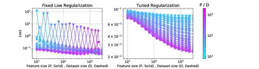
Figure S6: Duality between dataset size vs feature number in pretrained features Using pretrained embedding features of EfficientNet-B5 [tan2019efficientnet] for different levels of regularization, we see that loss as function of dataset size or loss as a function of the feature dimension track each other both for small regularization (left) and for tuned regularization (right). Note that regularization strength with trained-feature kernels can be mapped to inverse training time [ali2019continuous, lee2020finite]. Thus (left) corresponds to long training time and exhibits double descent behavior, while (right) corresponds to optimal early stopping.

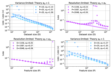
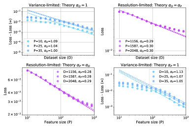
Figure S7: Four scaling regimes exhibited by pretrained embedding features Using pretrained embedding features of EfficientNet-B5 [tan2019efficientnet] for fixed low regularization (left) and tuned regularization (right), we can identify four regimes of scaling using real CIFAR-10 labels.

Expressions (S4) and (S5) are related by changing projections onto finite feature set, and finite dataset even without taking any asymptotic limits. We thus expect the dependence of test loss on parameter count and dataset size to be related quite generally in linear feature models. See Section E for further details.

Appendix E Learned Features

In this section, we consider linear models with features coming from pretrained neural networks. Such features are useful for transfer learning applications (e.g. kornblith2019better, kolesnikov2019big). In Figures S6 and S7, we take pretrained embedding features from an EfficientNet-B5 model [tan2019efficientnet] using TF hub. The EfficientNet model is pretrained using the ImageNet dataset with input image size of $(456,456)$. To extract features for the $(32,32)$ CIFAR-10 images, we use bilinear resizing. We then train a linear classifier on top of the penultimate pretrained features. To explore the effect feature size, $P$, and dataset size $D$, we randomly subset the feature dimension and training dataset size and average over $5$ random seeds. Prediction on test points are obtained as a kernel ridge regression problem with linear kernel. We note that the regularization ridge parameter can be mapped to an inverse early-stopping time [ali2019continuous, lee2020finite] of a corresponding ridgeless model trained via gradient descent. Inference with low regularization parameter denotes training for long time while tuned regularization parameter is equivalent to optimal early stopping.

In Figure S7 we see evidence of all four scaling regimes for low regularization (left four) and optimal regularization (right four). We speculate that the deviation from the predicted variance-limited exponent $\alpha_{P}=\alpha_{D}=1$ for the case of fixed low regularization (late time) is possibly due to the double descent resonance at $D=P$ which interferes with the power law fit.

In Figure S6, we observe the duality between dataset size $D$ (solid) and feature size $P$ (dashed) – the loss as a function of the number of features is identical to the loss as function of dataset size for both the optimal loss (tuned regularization) or late time loss (low regularization).

In Figure S8, we also compare properties of random features (using the infinite-width limit) and learned features from trained WRN 28-10 models. We note that teacher-student models, where the feature class matches the target function and ordinary, fully trained models on real data (Figure 1), have significantly larger exponents than models with fixed features and realistic targets.

The measured $\bar{\omega}_{i}$ – the coefficient of the task labels under the $i$-th feature (S12) are approximately constant as function of index $i$ for all teacher-student settings. However for real targets, $\bar{\omega}_{i}$ are only constant for the well-performing Myrtle-10 and WRN trained features (last two columns).

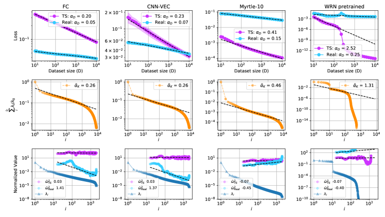
Figure S8: Loss on the teacher targets scale better than real targets for both untrained and trained features The first three columns are infinite width kernels while the last column is a kernel built out of features from the penultimate layer of pretrained WRN 28-10 models on CIFAR-10. The first row is the loss as a function of dataset size $D$ for teacher-student targets vs real targets. The observed dataset scaling exponent is denoted in the legend. The second row is the normalized partial sum of kernel eigenvalues. The partial sum’s scaling exponent is measured to capture the effect of the finite dataset size when empirical $\alpha_{K}$ is close to zero. The third row shows $\bar{\omega}_{i}$ for teacher-student and real target compared against the kernel eigenvalue decay. We see the teacher-student $\bar{\omega}_{i}$ are approximately constant.

References

- Hestness et al. [2017] Joel Hestness, Sharan Narang, Newsha Ardalani, Gregory Diamos, Heewoo Jun, Hassan Kianinejad, Md Patwary, Mostofa Ali, Yang Yang, and Yanqi Zhou. Deep learning scaling is predictable, empirically. arXiv preprint arXiv:1712.00409, 2017.
- Kaplan et al. [2020] Jared Kaplan, Sam McCandlish, Tom Henighan, Tom B Brown, Benjamin Chess, Rewon Child, Scott Gray, Alec Radford, Jeffrey Wu, and Dario Amodei. Scaling laws for neural language models. arXiv preprint arXiv:2001.08361, 2020.
- Rosenfeld et al. [2020a] Jonathan S. Rosenfeld, Amir Rosenfeld, Yonatan Belinkov, and Nir Shavit. A constructive prediction of the generalization error across scales. In International Conference on Learning Representations, 2020a.
- Henighan et al. [2020] Tom Henighan, Jared Kaplan, Mor Katz, Mark Chen, Christopher Hesse, Jacob Jackson, Heewoo Jun, Tom B. Brown, Prafulla Dhariwal, Scott Gray, Chris Hallacy, Benjamin Mann, Alec Radford, Aditya Ramesh, Nick Ryder, Daniel M. Ziegler, John Schulman, Dario Amodei, and Sam McCandlish. Scaling laws for autoregressive generative modeling. arXiv preprint arXiv:2010.14701, 2020.
- Rosenfeld et al. [2020b] Jonathan S. Rosenfeld, Jonathan Frankle, Michael Carbin, and Nir Shavit. On the predictability of pruning across scales. arXiv preprint arXiv:2006.10621, 2020b.
- Ahmad and Tesauro [1989] Subutai Ahmad and Gerald Tesauro. Scaling and generalization in neural networks: a case study. In Advances in neural information processing systems, pages 160–168, 1989.
- Cohn and Tesauro [1991] David Cohn and Gerald Tesauro. Can neural networks do better than the vapnik-chervonenkis bounds? In Advances in Neural Information Processing Systems, pages 911–917, 1991.
- Sharma and Kaplan [2020] Utkarsh Sharma and Jared Kaplan. A neural scaling law from the dimension of the data manifold. arXiv preprint arXiv:2004.10802, 2020.
- Neal [1994] Radford M. Neal. Bayesian Learning for Neural Networks. PhD thesis, University of Toronto, Dept. of Computer Science, 1994.
- Lee et al. [2018] Jaehoon Lee, Yasaman Bahri, Roman Novak, Sam Schoenholz, Jeffrey Pennington, and Jascha Sohl-dickstein. Deep neural networks as Gaussian processes. In International Conference on Learning Representations, 2018.
- Matthews et al. [2018] Alexander G. de G. Matthews, Jiri Hron, Mark Rowland, Richard E. Turner, and Zoubin Ghahramani. Gaussian process behaviour in wide deep neural networks. In International Conference on Learning Representations, 2018.
- Jacot et al. [2018] Arthur Jacot, Franck Gabriel, and Clement Hongler. Neural Tangent Kernel: Convergence and generalization in neural networks. In Advances in Neural Information Processing Systems, 2018.
- Lee et al. [2019] Jaehoon Lee, Lechao Xiao, Samuel S. Schoenholz, Yasaman Bahri, Roman Novak, Jascha Sohl-Dickstein, and Jeffrey Pennington. Wide neural networks of any depth evolve as linear models under gradient descent. In Advances in Neural Information Processing Systems, 2019.
- Dyer and Gur-Ari [2020] Ethan Dyer and Guy Gur-Ari. Asymptotics of wide networks from feynman diagrams. In International Conference on Learning Representations, 2020. URL https://openreview.net/forum?id=S1gFvANKDS.
- Spigler et al. [2020] Stefano Spigler, Mario Geiger, and Matthieu Wyart. Asymptotic learning curves of kernel methods: empirical data versus teacher–student paradigm. Journal of Statistical Mechanics: Theory and Experiment, 2020(12):124001, 2020.
- Bordelon et al. [2020] Blake Bordelon, Abdulkadir Canatar, and Cengiz Pehlevan. Spectrum dependent learning curves in kernel regression and wide neural networks. In International Conference on Machine Learning, pages 1024–1034. PMLR, 2020.
- Hutter [2021] Marcus Hutter. Learning curve theory. arXiv preprint arXiv:2102.04074, 2021.
- Rahimi and Recht [2008] Ali Rahimi and Benjamin Recht. Weighted sums of random kitchen sinks: replacing minimization with randomization in learning. In Nips, pages 1313–1320. Citeseer, 2008.
- Hastie et al. [2019] Trevor Hastie, Andrea Montanari, Saharon Rosset, and Ryan J Tibshirani. Surprises in high-dimensional ridgeless least squares interpolation. arXiv preprint arXiv:1903.08560, 2019.
- d’Ascoli et al. [2020] Stéphane d’Ascoli, Maria Refinetti, Giulio Biroli, and Florent Krzakala. Double trouble in double descent: Bias and variance (s) in the lazy regime. In International Conference on Machine Learning, pages 2280–2290. PMLR, 2020.
- Advani and Saxe [2017] Madhu S Advani and Andrew M Saxe. High-dimensional dynamics of generalization error in neural networks. arXiv preprint arXiv:1710.03667, 2017.
- Advani et al. [2020] Madhu S Advani, Andrew M Saxe, and Haim Sompolinsky. High-dimensional dynamics of generalization error in neural networks. Neural Networks, 132:428–446, 2020.
- Mei and Montanari [2019] Song Mei and Andrea Montanari. The generalization error of random features regression: Precise asymptotics and double descent curve. arXiv preprint arXiv:1908.05355, 2019.
- Adlam and Pennington [2020a] Ben Adlam and Jeffrey Pennington. The Neural Tangent Kernel in high dimensions: Triple descent and a multi-scale theory of generalization. In International Conference on Machine Learning, pages 74–84. PMLR, 2020a.
- Adlam and Pennington [2020b] Ben Adlam and Jeffrey Pennington. Understanding double descent requires a fine-grained bias-variance decomposition. Advances in Neural Information Processing Systems, 33, 2020b.
- Andreassen and Dyer [2020] Anders Andreassen and Ethan Dyer. Asymptotics of wide convolutional neural networks. arxiv preprint arXiv:2008.08675, 2020.
- Geiger et al. [2020] Mario Geiger, Arthur Jacot, Stefano Spigler, Franck Gabriel, Levent Sagun, Stéphane d’Ascoli, Giulio Biroli, Clément Hongler, and Matthieu Wyart. Scaling description of generalization with number of parameters in deep learning. Journal of Statistical Mechanics: Theory and Experiment, 2020(2):023401, 2020.
- Weyl [1912] Hermann Weyl. Das asymptotische verteilungsgesetz der eigenwerte linearer partieller differentialgleichungen (mit einer anwendung auf die theorie der hohlraumstrahlung). Mathematische Annalen, 71(4):441–479, 1912.
- Reade [1983] JB Reade. Eigenvalues of positive definite kernels. SIAM Journal on Mathematical Analysis, 14(1):152–157, 1983.
- Kühn [1987] Thomas Kühn. Eigenvalues of integral operators with smooth positive definite kernels. Archiv der Mathematik, 49(6):525–534, 1987.
- Ferreira and Menegatto [2009] JC Ferreira and VA Menegatto. Eigenvalues of integral operators defined by smooth positive definite kernels. Integral Equations and Operator Theory, 64(1):61–81, 2009.
- Stein [1999] Michael L Stein. Interpolation of Spatial Data: Some Theory for Kriging. Springer Science & Business Media, 1999.
- Bickel et al. [2007] Peter J Bickel, Bo Li, et al. Local polynomial regression on unknown manifolds. In Complex datasets and inverse problems, pages 177–186. Institute of Mathematical Statistics, 2007.
- de Laat [2011] David de Laat. Approximating manifolds by meshes: asymptotic bounds in higher codimension. Master’s Thesis, University of Groningen, Groningen, 2011.
- Brown et al. [2020] Tom B Brown, Benjamin Mann, Nick Ryder, Melanie Subbiah, Jared Kaplan, Prafulla Dhariwal, Arvind Neelakantan, Pranav Shyam, Girish Sastry, Amanda Askell, et al. Language models are few-shot learners. arXiv preprint arXiv:2005.14165, 2020.
- Fedus et al. [2021] William Fedus, Barret Zoph, and Noam Shazeer. Switch transformers: Scaling to trillion parameter models with simple and efficient sparsity, 2021.
- Yaida [2020] Sho Yaida. Non-Gaussian processes and neural networks at finite widths. In Mathematical and Scientific Machine Learning Conference, 2020.
- Hanin and Nica [2020] Boris Hanin and Mihai Nica. Finite depth and width corrections to the neural tangent kernel. In International Conference on Learning Representations, 2020. URL https://openreview.net/forum?id=SJgndT4KwB.
- Levina and Bickel [2005] Elizaveta Levina and Peter J Bickel. Maximum likelihood estimation of intrinsic dimension. In Advances in neural information processing systems, pages 777–784, 2005.
- McCullagh and Nelder [1989] P McCullagh and John A Nelder. Generalized Linear Models, volume 37. CRC Press, 1989.
- Rifkin and Lippert [2007] Ryan M Rifkin and Ross A Lippert. Notes on regularized least squares, 2007.
- Hastie et al. [2009] Trevor Hastie, Robert Tibshirani, and Jerome Friedman. The elements of statistical learning: data mining, inference, and prediction. Springer Science & Business Media, 2009.
- Goh [2017] Gabriel Goh. Why momentum really works. Distill, 2017. doi: 10.23915/distill.00006. URL http://distill.pub/2017/momentum.
- Nakkiran [2019] Preetum Nakkiran. More data can hurt for linear regression: Sample-wise double descent. arXiv preprint arXiv:1912.07242, 2019.
- Grosse [2021] Roger Grosse. University of Toronto CSC2541 winter 2021 neural net training dynamics, lecture notes, 2021. URL https://www.cs.toronto.edu/~rgrosse/courses/csc2541_2021.
- Novak et al. [2019] Roman Novak, Lechao Xiao, Jaehoon Lee, Yasaman Bahri, Greg Yang, Jiri Hron, Daniel A. Abolafia, Jeffrey Pennington, and Jascha Sohl-Dickstein. Bayesian deep convolutional networks with many channels are gaussian processes. In International Conference on Learning Representations, 2019.
- Garriga-Alonso et al. [2019] Adrià Garriga-Alonso, Laurence Aitchison, and Carl Edward Rasmussen. Deep convolutional networks as shallow gaussian processes. In International Conference on Learning Representations, 2019.
- Yang [2019] Greg Yang. Scaling limits of wide neural networks with weight sharing: Gaussian process behavior, gradient independence, and neural tangent kernel derivation. arXiv preprint arXiv:1902.04760, 2019.
- Lewkowycz et al. [2020] Aitor Lewkowycz, Yasaman Bahri, Ethan Dyer, Jascha Sohl-Dickstein, and Guy Gur-Ari. The large learning rate phase of deep learning: the catapult mechanism. arXiv preprint arXiv:2003.02218, 2020.
- Huang et al. [2020] Wei Huang, Weitao Du, Richard Yi Da Xu, and Chunrui Liu. Implicit bias of deep linear networks in the large learning rate phase. arXiv preprint arXiv:2011.12547, 2020.
- Chizat et al. [2019] Lenaic Chizat, Edouard Oyallon, and Francis Bach. On lazy training in differentiable programming. In Advances in Neural Information Processing Systems, pages 2937–2947, 2019.
- Loukas [2017] Andreas Loukas. How close are the eigenvectors of the sample and actual covariance matrices? In International Conference on Machine Learning, pages 2228–2237. PMLR, 2017.
- Canatar et al. [2020] Abdulkadir Canatar, Blake Bordelon, and Cengiz Pehlevan. Statistical mechanics of generalization in kernel regression. arXiv preprint arXiv:2006.13198, 2020.
- Zagoruyko and Komodakis [2016] Sergey Zagoruyko and Nikos Komodakis. Wide residual networks. In British Machine Vision Conference, 2016.
- Nakkiran and Bansal [2020] Preetum Nakkiran and Yamini Bansal. Distributional generalization: A new kind of generalization. arXiv preprint arXiv:2009.08092, 2020.
- Grathwohl et al. [2020] Will Grathwohl, Kuan-Chieh Wang, Joern-Henrik Jacobsen, David Duvenaud, Mohammad Norouzi, and Kevin Swersky. Your classifier is secretly an energy based model and you should treat it like one. In International Conference on Learning Representations, 2020. URL https://openreview.net/forum?id=Hkxzx0NtDB.
- Novak et al. [2020] Roman Novak, Lechao Xiao, Jiri Hron, Jaehoon Lee, Alexander A. Alemi, Jascha Sohl-Dickstein, and Samuel S. Schoenholz. Neural Tangents: Fast and easy infinite neural networks in python. In International Conference on Learning Representations, 2020. URL https://github.com/google/neural-tangents.
- Bradbury et al. [2018] James Bradbury, Roy Frostig, Peter Hawkins, Matthew James Johnson, Chris Leary, Dougal Maclaurin, George Necula, Adam Paszke, Jake VanderPlas, Skye Wanderman-Milne, and Qiao Zhang. JAX: composable transformations of Python+NumPy programs, 2018. URL http://github.com/google/jax.
- Shankar et al. [2020] Vaishaal Shankar, Alex Chengyu Fang, Wenshuo Guo, Sara Fridovich-Keil, Ludwig Schmidt, Jonathan Ragan-Kelley, and Benjamin Recht. Neural kernels without tangents. In International Conference on Machine Learning, 2020.
- Schoenholz et al. [2017] Samuel S Schoenholz, Justin Gilmer, Surya Ganguli, and Jascha Sohl-Dickstein. Deep information propagation. International Conference on Learning Representations, 2017.
- Xiao et al. [2018] Lechao Xiao, Yasaman Bahri, Jascha Sohl-Dickstein, Samuel Schoenholz, and Jeffrey Pennington. Dynamical isometry and a mean field theory of CNNs: How to train 10,000-layer vanilla convolutional neural networks. In International Conference on Machine Learning, 2018.
- Heek et al. [2020] Jonathan Heek, Anselm Levskaya, Avital Oliver, Marvin Ritter, Bertrand Rondepierre, Andreas Steiner, and Marc van Zee. Flax: A neural network library and ecosystem for JAX, 2020. URL http://github.com/google/flax.
- Ritchie et al. [2020] Sam Ritchie, Ambrose Slone, and Vinay Ramasesh. Caliban: Docker-based job manager for reproducible workflows. Journal of Open Source Software, 5(53):2403, 2020. doi: 10.21105/joss.02403. URL https://doi.org/10.21105/joss.02403.
- Loshchilov and Hutter [2016] Ilya Loshchilov and Frank Hutter. Sgdr: Stochastic gradient descent with warm restarts. arXiv preprint arXiv:1608.03983, 2016.
- Paszke et al. [2019] Adam Paszke, Sam Gross, Francisco Massa, Adam Lerer, James Bradbury, Gregory Chanan, Trevor Killeen, Zeming Lin, Natalia Gimelshein, Luca Antiga, et al. Pytorch: An imperative style, high-performance deep learning library. Advances in Neural Information Processing Systems, 32:8026–8037, 2019.
- Williams and Vivarelli [2000] Christopher KI Williams and Francesco Vivarelli. Upper and lower bounds on the learning curve for gaussian processes. Machine Learning, 40(1):77–102, 2000.
- Malzahn and Opper [2002] Dörthe Malzahn and Manfred Opper. A variational approach to learning curves. In T. Dietterich, S. Becker, and Z. Ghahramani, editors, Advances in Neural Information Processing Systems, volume 14, pages 463–469. MIT Press, 2002. URL https://proceedings.neurips.cc/paper/2001/file/26f5bd4aa64fdadf96152ca6e6408068-Paper.pdf.
- Sollich and Halees [2002] Peter Sollich and Anason Halees. Learning curves for gaussian process regression: Approximations and bounds. Neural computation, 14(6):1393–1428, 2002.
- Parisi [1980] Giorgio Parisi. A sequence of approximated solutions to the sk model for spin glasses. Journal of Physics A: Mathematical and General, 13(4):L115, 1980.
- Sollich [1998] Peter Sollich. Learning curves for gaussian processes. In Proceedings of the 11th International Conference on Neural Information Processing Systems, pages 344–350, 1998.
- Malzahn and Opper [2001] Dörthe Malzahn and Manfred Opper. Learning curves for gaussian processes regression: A framework for good approximations. Advances in neural information processing systems, pages 273–279, 2001.
- Malzahn and Opper [2003] Dörthe Malzahn and Manfred Opper. Learning curves and bootstrap estimates for inference with gaussian processes: A statistical mechanics study. Complexity, 8(4):57–63, 2003.
- Urry and Sollich [2012] Matthew J Urry and Peter Sollich. Replica theory for learning curves for gaussian processes on random graphs. Journal of Physics A: Mathematical and Theoretical, 45(42):425005, 2012.
- Cohen et al. [2019] Omry Cohen, Or Malka, and Zohar Ringel. Learning curves for deep neural networks: a gaussian field theory perspective. arXiv preprint arXiv:1906.05301, 2019.
- Gerace et al. [2020] Federica Gerace, Bruno Loureiro, Florent Krzakala, Marc Mézard, and Lenka Zdeborová. Generalisation error in learning with random features and the hidden manifold model. In International Conference on Machine Learning, pages 3452–3462. PMLR, 2020.
- Tan and Le [2019] Mingxing Tan and Quoc Le. Efficientnet: Rethinking model scaling for convolutional neural networks. In International Conference on Machine Learning, pages 6105–6114. PMLR, 2019.
- Ali et al. [2019] Alnur Ali, J Zico Kolter, and Ryan J Tibshirani. A continuous-time view of early stopping for least squares regression. In The 22nd International Conference on Artificial Intelligence and Statistics, pages 1370–1378, 2019.
- Lee et al. [2020] Jaehoon Lee, Samuel Schoenholz, Jeffrey Pennington, Ben Adlam, Lechao Xiao, Roman Novak, and Jascha Sohl-Dickstein. Finite versus infinite neural networks: an empirical study. Advances in Neural Information Processing Systems, 33, 2020.
- Kornblith et al. [2019] Simon Kornblith, Jonathon Shlens, and Quoc V Le. Do better imagenet models transfer better? In Proceedings of the IEEE/CVF Conference on Computer Vision and Pattern Recognition, pages 2661–2671, 2019.
- Kolesnikov et al. [2019] Alexander Kolesnikov, Lucas Beyer, Xiaohua Zhai, Joan Puigcerver, Jessica Yung, Sylvain Gelly, and Neil Houlsby. Big transfer (bit): General visual representation learning. arXiv preprint arXiv:1912.11370, 6(2):8, 2019.