Coupled Sachdev–Ye–Kitaev models without Schwartzian dominance

Abstract

We argue that in certain class of coupled Sachdev–Ye–Kitaev(SYK) models the low energy physics at large $N$ is governed by a non-local action rather than the Schwartzian action. We present a partial analytic and extensive numerical evidence for this. We find that these models are maximally chaotic and have the same residual entropy as Majorana SYK. However, thermodynamic quantities, such as heat capacity and diffusion constant are different.

I Introduction

Recently Sachdev–Ye–Kitaev(SYK) model Sachdev and Ye (1993); Parcollet et al. (1998); Georges et al. (2001); Kitaev ; Gross and Rosenhaus (2016) and tensor models Gurau (2011); Witten (2016); Klebanov and Tarnopolsky (2017a, b) have been the focus of much theoretical research. Also there have been several proposal of possible experimental implementation Chew et al. (2017); Danshita et al. (2017); Chen et al. (2018); Can et al. (2019); Wei and Sedrakyan (2021). The most prominent features of this family of models are non-Fermi liquid behavior, maximal Maldacena et al. (2015) Lyapunov exponent, non-zero residual entropy and an approximate time reparametrization symmetry at large $N$ and low energies. Maldacena and Stanford Maldacena and Stanford (2016) and Kitaev and Suh Kitaev and Suh (2018) derived the following (Euclidean) Schwartzian action for reparametrizations in the original SYK model:

$$S_{Sch}=-\frac{N\alpha^{S}_{Sch}}{J}\int du\ \operatorname*{Sch}\left(\tau[u],u\right),$$ (1)

$$\operatorname*{Sch}\left(\tau[u],u\right)=\frac{\tau^{\prime\prime\prime}}{\tau^{\prime}}-\frac{3}{2}\left(\frac{\tau^{\prime\prime}}{\tau^{\prime}}\right)^{2}$$

In all known SYK-like modes, the Schwartzian has been identified as the dominant low-energy action and its physics has been explored in a variety of situations Maldacena and Qi (2018); Fu et al. (2016); Cotler et al. (2017); Gu et al. (2017a); Yoon (2017); Gur-Ari et al. (2018); Maldacena and Milekhin (2019); Almheiri et al. (2019); Chen et al. (2017); Zhang (2019); Gu et al. (2019); Su et al. (2021). In this Letter we present a coupled SYK model which is dominated by the following non-local action instead of the Schwartzian action:

$$S_{nonloc}=-\frac{N\alpha^{S}_{2h}}{J^{2h-2}}\int du_{1}du_{2}\left(\frac{\tau^{\prime}(u_{1})\tau^{\prime}(u_{2})}{(\tau(u_{1})-\tau(u_{2}))^{2}}\right)^{h}$$ (2)

It was suggested by Maldacena, Stanford and Yang Maldacena et al. (2016) that this action may appear when a theory contains a local irrelevant operator with the dimension $h$ within the interval $1<h<3/2$. Holographically this corresponds to a light matter field in $AdS_{2}$ having a source term at the boundary. In our model $h$ is tunable and can be anywhere between $1$ and $2$.

We would like to stress that the Schwartzian term is still present in our model. The key point is that at large $N$ it gives a subleading in $T/J$ contribution, where $T$ is the temperature.

Our approach is semi-analytical. We consider strict large $N$ limit and obtain various predictions of the non-local action. Then we check them against numerical solutions of exact large $N$ equations. Also we demonstrate that the Lyapunov exponent is still maximal and study the transport in chain models. In the accompanying longer paper Milekhin we provide more details on numerics and theoretical computations, explore other aspects of these models and study $1/N$ corrections.

II Microscopic formulation

The model consists of two independent Majorana SYK models($\mathcal{L}_{kin}+\mathcal{L}_{SYK}$), a marginal interaction($\mathcal{L}_{int}$) between them, and an innocuously-looking kinetic term twist($\mathcal{L}_{\xi}$):

$$\mathcal{L}_{T}=\mathcal{L}_{kin}+\mathcal{L}_{SYK}+\mathcal{L}_{int}+\mathcal{L}_{\xi},$$ (3)

where

$$\mathcal{L}_{kin}=\frac{1}{2}\sum_{i}\left(\psi^{1}_{i}\partial_{u}\psi^{1}_{i}+\psi^{2}_{i}\partial_{u}\psi^{2}_{i}\right)$$ (4)

$$\mathcal{L}_{SYK}=\frac{1}{4!}\sum_{ijkl}\Bigg{(}J^{1}_{ijkl}\psi^{1}_{i}\psi^{1}_{j}\psi^{1}_{k}\psi^{1}_{l}+J^{2}_{ijkl}\psi^{2}_{i}\psi^{2}_{j}\psi^{2}_{k}\psi^{2}_{l}\Bigg{)}$$ (5)

$$\mathcal{L}_{int}=\frac{3}{2}\alpha\sum_{ijkl}C_{ij;kl}\psi^{1}_{i}\psi^{1}_{j}\psi^{2}_{k}\psi^{2}_{l}$$ (6)

$$\mathcal{L}_{\xi}=-\frac{\xi}{2}\sum_{i}\left(\psi^{1}_{i}\partial_{u}\psi^{1}_{i}-\psi^{2}_{i}\partial_{u}\psi^{2}_{i}\right)$$ (7)

There are $2N$ Majorana fermions $\psi^{a}_{i},\ i=1,\dots,N,\ a=1,2$. This action with $\xi=0$ has been studied in the literature before Gu et al. (2017b); Altland et al. (2019); Chen et al. (2017) and it was argued that it is dominated by the Schwartzian. It is important that tensors $J^{1,2},C$ are different. When they are the same the ground state is actually gapped and the model is prone to $\mathbb{Z}_{2}$ symmetry breaking Kim et al. (2019). Low energy physics is not described by the conformal solution in this case. We will give a brief analytical argument below why this does not happen in our model. Also we cross-checked this with exact diagonalization Milekhin at finite $N$. The non-local action emerges only when both $\alpha\neq 0,\xi\neq 0$. Non-zero $\alpha$ renders the two SYK models coupled and also it controls the dimension $h$ in the non-local action. Specifically, we need $|\alpha|>1$ to make the non-local action dominant. Non-zero $\xi$ explicitly breaks $\psi^{1}_{i}\leftrightarrow\psi^{2}_{i}$ $\mathbb{Z}_{2}$ symmetry and the needed irrelevant operator appears in the conformal perturbation theory(more on it below). Tensors $J^{1},J^{2}$, are standard SYK disorders(totally antisymmetric with i.i.d. Gaussian components). Tensor $C_{ij;kl}$ has a Gaussian distribution too, but it has a separate skew-symmetry in $ij$ and $kl$ indices:

$$C_{ij;kl}=-C_{ji;kl}=-C_{ij;lk}$$ (8)

With the variances:

$$\langle\left(J^{a}_{ijkl}\right)^{2}\rangle=\frac{3!J^{2}}{N^{3}},\ a=1,2;\ \langle\left(C_{ij;kl}\right)^{2}\rangle=\frac{J^{2}}{6N^{3}}$$ (9)

Euclidean Schwinger–Dyson(SD) equations read

$$(1-\xi)\partial_{u}G_{11}-J^{2}(G_{11}^{3}+3\alpha^{2}G_{11}G_{22}^{2})*G_{11}=\delta(u)$$

$$(1+\xi)\partial_{u}G_{22}-J^{2}(G_{22}^{3}+3\alpha^{2}G_{22}G_{11}^{2})*G_{22}=\delta(u)$$ (10)

with $*$ denoting time convolution. $G_{11/22}$ are the time-ordered Green functions:

$$G_{aa}(u)=\langle T\psi^{a}_{i}(u)\psi^{a}_{i}(0)\rangle,\ a=1,2$$ (11)

In principle, $\xi$ can be reabsorbed into $J^{1},J^{2}$ variances. Mixed correlators $\langle\psi^{1}_{i}\psi^{2}_{i}\rangle$ do not appear up to $1/N$ order. These correlators serve as order parameters for the gapped $\mathbb{Z}_{2}$-symmetry broken phase. This suggests that this breaking does not happen in our model and the physics can be described by the following conformal solution. At low energies we can neglect the kinetic term and $\xi$ disappears. Assuming $G_{11}=G_{22}$, one obtains the familiar SYK conformal solution

$$G_{11,22}=G_{conf}=\frac{b\operatorname*{sgn}(u)}{(1+3\alpha^{2})^{1/4}}\frac{\pi}{\sqrt{J\beta\sin\left(\frac{\pi|u|}{\beta}\right)}}$$ (12)

with $b=1/(4\pi)^{1/4}$. The full solution can be obtained by numerically solving SD equations. Our numerical approach is a simple iteration procedure commonly used in SYK literature Maldacena and Stanford (2016). We cross-checked our numerical solution against the results of exact diagonalization at finite $N$ Milekhin .

It is important that the equations are coupled, so there is only one reparametrization mode. Time reparametrizations act on Green functions by

$$G_{aa}(u_{1},u_{2})\rightarrow\left(\tau(u_{1})^{\prime}\tau(u_{2})^{\prime}\right)^{1/4} G_{aa}(\tau(u_{1}),\tau(u_{2})),$$

$$a=1,2$$ (13)

This equation implies that $\psi$ have conformal dimension $1/4$. It is easy to compute the dimension $h$ of the following bilinear operator Kim et al. (2019):

$$\mathcal{O}_{2,0}=\sum_{i}\left(\psi^{1}_{i}\partial_{u}\psi^{1}_{i}-\psi^{2}_{i}\partial_{u}\psi^{2}_{i}\right),$$ (14)

it is given by the smallest solution of

$$\frac{1-\alpha^{2}}{1+3\alpha^{2}}g_{A}(h)=1,\quad g_{A}(h)=-\frac{3}{2}\frac{\tan\left(\pi(h-1/2)/2\right)}{h-1/2}$$ (15)

For $|\alpha|>1$, the dimension $h$ is in the range: $1<h<3/2$. This bilinear operator is exactly the $\mathcal{L}_{\xi}$ term in the Lagrangian.

III A perturbative argument

As in the standard SYK, we can go beyond the conformal sector by perturbing Kitaev and Suh (2018); Tikhanovskaya et al. (2020) the exact conformal Lagrangian

$$\mathcal{L}_{conf}=\mathcal{L}_{SYK}+\mathcal{L}_{int}$$ (16)

by a set of irrelevant operators

$$\mathcal{L}_{T}=\mathcal{L}_{conf}+\sum_{h}\alpha_{h}\mathcal{O}_{h}$$ (17)

Unfortunately, there is no ab initio way to compute $\alpha_{h}$. The set of these irrelevant operators is constrained by the symmetries of the model. For $\xi=0$ there is $1\leftrightarrow 2$ symmetry at large $N$ and the operator (14) does not appear. This is why we need the $\mathcal{L}_{\xi}$ term in the UV Lagrangian. However, the corresponding IR parameter $\alpha_{h}$ does not have to be linear in $\xi$ Milekhin . Now we can see the origin of the non-local action (2). In perturbation theory, one can derive it by taking the 2-point function of $\mathcal{O}_{h}$ and dressing it with reparametrizations Maldacena et al. (2016). Higher-order terms are suppressed by $1/N$. This agrees with holographic expectations of weakly interacting fields in the bulk in the large $N$ limit. Another consequence of this formalism is the leading non-conformal correction to the 2-point function:

$$\delta G_{11}(u)=\alpha_{h}\int du^{\prime}\ \langle\mathcal{O}_{h}(u^{\prime})\psi^{1}_{i}(u)\psi^{1}_{i}(0)\rangle\propto\frac{1}{(Ju)^{h-1/2}}$$ (18)

The last equality is valid for $|u|\ll\beta$. We checked this prediction by numerically computing the spectral density at zero temperature and real frequency:

$$\rho_{11/22}(\omega)=\operatorname{Im}G_{R,11/22}(\omega),$$ (19)

where $G_{R}$ is retarded Green function. Conformal behavior (12) results in $\rho\sim 1/\sqrt{\omega}$ for $\omega\ll J$, whereas the non-conformal correction (18) gives $\rho\sim\omega^{h-3/2}$. Therefore, we expect the following behavior at small $\omega$:

$$\sqrt{\omega}\rho_{11/22}=b_{1}\pm b_{2}\omega^{h-1}$$ (20)

Constant $b_{1}$ can be extracted from the conformal solution, but $b_{2}$ is related to $\alpha_{h}$ and has to be extracted from the numerics. The result is presented in Figure 1. We see a good agreement with the numerical results.

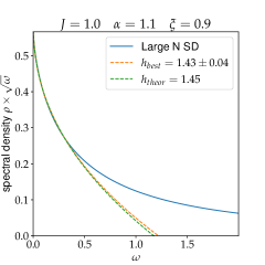
Figure 1: Results for $G_{11}$. The fit was performed with $b_{1}+b_{2}\omega^{h-1}$. Uncertainty in $h_{best}$ results from changing the fitting interval. Theoretical $h$ is obtained from eq. (15).

IV Thermodynamics

Due to overall $N$ factor, we can treat the non-local action (2) classically as long as $T\gg J/N^{1/(2h-2)}$. Its contribution to free energy is equal to the classical action evaluated on the thermal solution $\tau(u)=\tan(\pi u/\beta)$. This computation produces a divergence Maldacena et al. (2016):

$$-\frac{\Delta F_{nonloc}}{N}=\#+T^{2h-1}\frac{\alpha_{2h}^{S}\pi^{2h-1/2}}{J^{2h-2}}\frac{\Gamma\left(1/2-h\right)}{\Gamma\left(1-h\right)}$$ (21)

where we assumed a fixed cut-off $u\sim 1/J$ in Euclidean time. The divergent term $\#$ is temperature-independent and shifts the ground state energy, and so we drop it. Adding the Schwartzian contribution, we get the following answer for thermodynamic energy:

$$E/N=E_{0}+c_{2h}T^{2h-1}+\frac{2\pi^{2}\alpha^{S}_{Sch}}{J}T^{2}+\dots$$ (22)

where

$$c_{2h}=(2h-2)\frac{\alpha_{2h}^{S}\pi^{2h-1/2}}{J^{2h-2}}\frac{\Gamma\left(1/2-h\right)}{\Gamma\left(1-h\right)}$$ (23)

For $1<h<3/2$ the non-local piece dominates over the Schwartzian at low temperatures. It is straightforward to extract the thermodynamic energy from numerically computed $G_{11}$ and $G_{22}$. The comparison between the prediction (22) and the numerics is shown in Figure 2, which demonstrates good agreement.

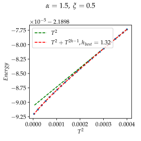
Figure 2: Energy $E/N$ vs $T^{2}$ for $J=2\pi$. Blue points are numerical data. There is a clear deviation from Schwartzian $T^{2}$ prediction. For $\alpha=1.5$, $h_{theor}=1.31$. Altering temperature range($\beta=50,\dots,500$), the number of (uniform) discretization points($2^{23}-2^{26}$) and removing $c_{Sch}T^{2}$ term results in $h_{best}=1.32\pm 0.02$. The fit was performed using eq. (22) with unknown $E_{0},c_{2h},c_{Sch}$.

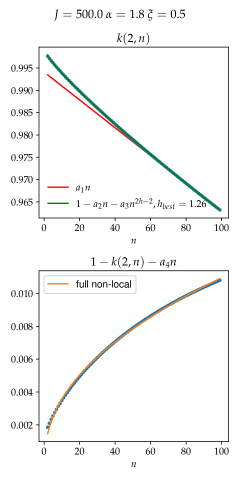
Figure 3: Results for $k(2,n)$. Blue points are numerically obtained eigenvalues of $K_{n}$ in eq. (25). Top: since $g_{h}(n)$ is actually numerically close to $n^{2h+1}$, we have performed the fit with $1-a_{2}n-a_{3}n^{2h-2}$ at large $n$ to extract $h_{best}$. For $\alpha=1.8$, $h_{theor}=1.24$, whereas $h_{best}=1.28\pm 0.04$ Bottom: fit with eq. (26) with $\alpha^{K}_{Sch,2h}$ unknown: $a_{4}=\alpha^{K}_{Sch}/\beta J$.

Conformal solution (12) has the same form as in the original SYK. Zero temperature residual entropy can be extracted from the conformal solution Parcollet et al. (1998); Gu et al. (2019). Hence the residual entropy should be twice Majorana SYK residual entropy. Our numerical results support this claim.

V Kernel and 4-point function

As in the original SYK, connected 4-point function $\mathcal{F}$ is given by a sum of ladder diagrams: $\mathcal{F}\propto 1/(1-K)$. ”Flavor” indices $1,2$ turn the kernel $K$ into $2\times 2$ matrix. It is the most convenient to represent it by its action on vector $v=(v_{1},v_{2})$:

$$\frac{Kv}{3J^{2}}=\begin{pmatrix}G_{11}*\left(\left(G_{11}^{2}+\alpha^{2}G_{22}^{2}\right)v_{1}+\ 2\alpha^{2}G_{11}G_{22}v_{2}\right)*G_{11}\\ G_{22}*\left(\left(G_{22}^{2}+\alpha^{2}G_{11}^{2}\right)v_{2}+\ 2\alpha^{2}G_{11}G_{22}v_{1}\right)*G_{22}\\ \end{pmatrix}$$ (24)

Using the translation symmetry, it is possible to separate the Matsubara frequency $n$ and re-write the kernel as a function of two times only Gu et al. (2019):

$$K_{n,ab}(u,u^{\prime})=\int_{0}^{\beta}dsK_{ab}\left(s+\frac{u}{2},s-\frac{u}{2};\frac{u^{\prime}}{2},-\frac{u^{\prime}}{2}\right)e^{-2\pi ins/\beta}$$ (25)

Because of the reparametrizations, this kernel has eigenvalue $1$ in the conformal approximation for any integer $n$ except $0,\pm 1$. The eigenvalue shift $1-k(2,n)$ can be read off from the reparametrization action:

$$1-k(2,n)=\frac{\alpha^{K}_{2h}}{(\beta J)^{2h-2}}\frac{g_{h}(n)}{|n|(n^{2}-1)}+\frac{\alpha^{K}_{Sch}|n|}{\beta J}$$ (26)

$$g_{h}(n)=n^{2}\left(\frac{\Gamma(n+h)}{\Gamma(1+n-h)}-\frac{\Gamma(h-1)}{\Gamma(-h)}\right)$$ (27)

where the first term in $1-k(2,n)$ comes from the non-local action, and the second linear in $|n|$ term comes from the Schwartzian . The relation between $\alpha^{K}_{2h}$ and $\alpha^{S}_{2h}$ is

$$\alpha^{K}_{2h}=-(2\pi)^{2h+1}\frac{\pi(h-1)^{2}}{\cos(\pi h)\Gamma(2h)}\frac{4}{\pi^{4}b^{4}}\alpha^{S}_{2h}$$ (28)

Using the exact numerical solutions $G_{11,22}$ and fixing $\beta=2\pi$, we build the kernel (25) for each $n=2,\dots,100$ and found numerically the eigenvalue $k(2,n)$ closest to $1$. For this we used a uniform 2D grid in $(u,u^{\prime})$ plane with $60,000^{2}-140,000^{2}$ points. The comparison between the prediction (26) and the numerics is shown in Figure 3.

Performing the same procedure for different $J$, we verified $J^{2h-2}$ dependence in eq. (26) Milekhin . The eigenvalue shift is sensitive to exact form of reparametrization action. We take the high levels of agreement with the numerics as the main evidence for the non-local action dominance.

VI Chaos exponent

Let us demonstrate that the Lyapunov exponent is maximal in the out-of-time ordered correlation function (OTOC). We are interested in the connected 4-point function

$$\mathcal{F}=\langle\psi^{1}_{i}(u_{1})\psi^{1}_{i}(u_{2})\psi^{1}_{j}(u_{3})\psi^{1}_{j}(u_{4})\rangle_{conn}$$ (29)

in the OTOC region:

$$u_{1}=-\beta/4+it,u_{3}=0,\ u_{2}=\beta/4+it,u_{4}=\beta/2$$ (30)

The leading (in $1/\beta J$) contribution comes from averaging the disconnected 4-point function over the reparametrizations. Delegating details to the Supplementary Material, we write down the final answer for OTOC:

$$\mathcal{F}=-p_{h}\frac{(\beta J)^{2h-2}}{N\alpha^{S}_{2h}m_{h}}\exp\left(\frac{2\pi t}{\beta}\right)+[\text{non-increasing}]$$ (31)

with coefficient

$$p_{h}=\frac{\pi^{3-2h}\Gamma(2-h)}{4\Gamma(1+h)(\psi(1+h)-\psi(2-h))}G_{conf}(\beta/2)^{2}$$ (32)

and where $\psi(x)=\Gamma^{\prime}(x)/\Gamma(x)$. The Lyapunov exponent $2\pi t/\beta$ is maximal. However, the prefactor $(\beta J)^{2h-2}$ is smaller compared to Schwartzian-dominated original SYK, where it is $(\beta J)^{1}$.

VII Transport in chain models

We can arrange the coupled model into an array and study transport properties. In SYK chain models dominated by the Schwartzian Gu et al. (2017b); Song et al. (2017), the diffusion constant is temperature-independent and the heat conductivity is linear in the temperature. Here we find that the non-local action renders the diffusion constant temperature-dependent, but leaves the heat conductivity proportional to the temperature. Specifically, we consider the following construction - Figure 4:

$$\mathcal{L}_{T,chain}=\sum_{x}\mathcal{L}_{T,x}+\mathcal{L}_{int,chain}$$ (33)

where $\mathcal{L}_{T,x}$ is an independent copy of the coupled model (3). The interaction between the sites should be carefully chosen in order to avoid a possible spontaneous $\mathbb{Z}_{2}$ symmetry breaking. We study the following interaction term between the sites:

$$\mathcal{L}_{int,chain}=\frac{1}{2!^{2}}\sum_{x,ijkl}\Big{(}V^{1,x}_{ij;kl}\psi^{1}_{i,x}\psi^{1}_{j,x}\psi^{1}_{k,x+1}\psi^{1}_{l,x+1}+$$

$$V^{2,x}_{ij;kl}\psi^{2}_{i,x}\psi^{2}_{j,x}\psi^{2}_{k,x+1}\psi^{2}_{l,x+1}\Big{)}$$ (34)

Each $V^{1/2,x}_{ij;kl}$ i.i.d. Gaussian and is skew symmetric in $ij$ and $kl$:

$$V^{1/2,x}_{ij;kl}=-V^{1/2,x}_{ji;kl}=-V^{1/2,x}_{ij;lk},$$ (35)

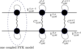
Figure 4: Illustration of couplings in the chain model.

and has $x-$independent variance

$$\langle\left(V^{1/2,x}_{ij;kl}\right)^{2}\rangle=\frac{V^{2}}{N^{3}}.$$ (36)

Assuming the two-point functions to be $x$-independent we arrive at single-site SD equations (II) with effective $\widetilde{J}$ and $\widetilde{\alpha}$:

$$\widetilde{J}^{2}=J^{2}+V^{2},\ \widetilde{\alpha}=\alpha\frac{J^{2}}{J^{2}+V^{2}}$$ (37)

It is important to keep in mind that the conformal dimension $h$ in the non-local action is now determined by this renormalized $\widetilde{\alpha}$. In Supplementary Material we derive the following low-energy action for reparametrizations:

$$S_{hydro}=\frac{\pi^{4}b^{4}N}{4}\frac{\beta}{2\pi}\int d\omega dp\ \epsilon_{\omega,p}\left(\frac{\alpha^{K}_{2h}}{(\beta\widetilde{J})^{2h-2}}\frac{(2h-1)\Gamma(h)}{\Gamma(2-h)}\frac{\omega^{2}\beta^{2}}{4\pi^{2}}+ip^{2}\frac{\omega\beta}{2\pi}\frac{V^{2}}{3\widetilde{J}^{2}(1+3\widetilde{\alpha}^{2})}\right)\epsilon_{-\omega,-p}$$ (38)

The action is valid in the hydrodynamic regime $\omega\ll T,p\ll 1$, where $p$ is the momentum conjugate to $x$. In this regime the reparametrization modes $\epsilon_{\omega,p}$ are proportional to stress-energy tensor Milekhin ; Song et al. (2017). We clearly see a diffusion pole in $\epsilon$ propagator with the diffusion coefficient:

$$D=T^{3-2h}\frac{2\pi\Gamma(2-h)}{3(2h-1)\Gamma(h)}\frac{V^{2}\widetilde{J}^{2h-2}}{\alpha^{K}_{2h}\widetilde{J}^{2}(1+3\widetilde{\alpha}^{2})}$$ (39)

This result differs a lot from SYK chains where the Schwartzian dominance results in temperature-independent diffusion constant. Standard hydrodynamic expectation is that thermal conductivity is given by diffusion constant times the heat capacity. This can be seen explicitly by the aforementioned mapping of $\epsilon_{\omega,p}$ to stress-energy tensor. In our case the heat capacity $c_{v}$ is proportional to $NT^{2h-2}$, eq. (22). Therefore the thermal conductivity is linear in the temperature, as in Schwartzian-dominated theories:

$$\kappa=c_{v}D\propto NT$$ (40)

VIII Conclusion

In this Letter we studied a coupled SYK model which shares a lot properties with the original SYK: the same conformal solution, residual entropy and maximal chaos exponent. However, in contrast to all known SYK-like models, the low energy physics at large $N$ is dominated by the non-local action for reparametrizations (2) instead of the Schwartzian action. The reason behind this is the presence of the light conformal field $\mathcal{O}_{2,0}$, eq. (14), with the dimension $h$, $1<h<3/2$. This conformal field is explicitly “brought to life” by the $\xi$ term in the Lagrangian (3). We would like to emphasize that this situation is not exotic: we studied the simplest coupled SYK and it is pretty easy to manipulate with conformal dimensions in the coupled SYK-like models Kim et al. (2019); Klebanov et al. (2020). Actually in our model for $|\alpha|<1$, the key operator $\mathcal{O}_{2,0}$, eq. (14), has the dimension $3/2<h<2$. This does not result in the dominance over the Schwartzian, but does result in the leading non-conformal correction being different from SYK Milekhin .

The non-local action, compared to the Schwartzian, produces a different heat capacity, eq. (22), OTOC prefactor, eq. (31), and temperature-dependent diffusion constant in chain models, eq. (39). Interestingly, the thermal conductivity is still linear in the temperature. This result suggests that this linearity is a more general feature which perhaps can be derived from the conformal solution. It would be very interesting to consider models with $U(1)$ symmetry and see if the electrical conductivity is linear in the temperature too as in strange metal.

Obviously, there are a lot of other open questions. There exists huge literature on SYK and the Schwartzian. Essentially, all the questions asked there could be asked for the non-local action. The most interesting of them is to study the strongly-coupled regime of this model, when the temperature $T\lesssim J/N^{1/(2h-2)}$ and the non-local action is not semiclassical. Up to non-perturbative $e^{-N}$ correction is this equivalent to quantizing 2D Jackiw–Teitelboim gravity on a disk with light matter fields.

IX Acknowledgment

The author is forever indebted to I. Klebanov, G. Tarnopolsky and W. Zhao for a lot of discussions and comments throughout this project. It is pleasure to thank A. Gorsky, J. Turiaci and especially D. Stanford and Z. Yang for comments, and F. Popov for useful input and insightful suggestions on the paper. I would like to thank C. King for moral support and help with the manuscript. This material is based upon work supported by the Air Force Office of Scientific Research under award number FA9550-19-1-0360. It was also supported in part by funds from the University of California. Use was made of computational facilities purchased with funds from the National Science Foundation (CNS-1725797) and administered by the Center for Scientific Computing (CSC). The CSC is supported by the California NanoSystems Institute and the Materials Research Science and Engineering Center (MRSEC; NSF DMR 1720256) at UC Santa Barbara.

Appendix A Supplementary material

A.1 OTOC computation

Averaging the product of two Green functions over the reparametrizations we get

$$\frac{\langle\psi^{1}_{i}(\theta_{1})\psi^{1}_{i}(\theta_{2})\psi^{1}_{j}(\theta_{3})\psi^{1}_{j}(\theta_{4})\rangle_{conn}}{G_{conf}(x)G_{conf}(x^{\prime})}=\frac{(\beta J)^{2h-2}}{N}\frac{\pi^{2-2h}}{2m_{h}\alpha_{2h}^{S}}\times$$

$$\times\sum_{|n|\geq 2}\frac{e^{in(y^{\prime}-y)}}{g_{h}(n)}\left[\frac{\sin\frac{nx}{2}}{\tan\frac{x}{2}}-n\cos\frac{nx}{2}\right]\left[\frac{\sin\frac{nx^{\prime}}{2}}{\tan\frac{x^{\prime}}{2}}-n\cos\frac{nx^{\prime}}{2}\right]$$ (41)

$\theta_{i}$ are variables on the thermal circle, $\theta=2\pi u/\beta$, and $y,y^{\prime},x,x^{\prime}$ are their combinations:

$$x=\theta_{1}-\theta_{2},\ x^{\prime}=\theta_{3}-\theta_{4},\ y=\frac{\theta_{1}+\theta_{2}}{2},\ y^{\prime}=\frac{\theta_{3}+\theta_{4}}{2}$$ (42)

The computation simplifies a lot for points antipodal on the thermal circle. For them

$$\theta_{1}=-\frac{\pi}{2}-\theta,\theta_{3}=0,\ \theta_{2}=\frac{\pi}{2}-\theta,\theta_{4}=\pi$$ (43)

Therefore we have the 4-point function (41) proportional to

$$\sum_{|n|\geq 2}\frac{e^{in\left(\pi/2+\theta\right)}n^{2}\cos^{2}\frac{\pi n}{2}}{g_{h}(n)}=\oint_{\mathcal{C}}dn\ \frac{n^{2}}{e^{i\pi n}-1}\frac{e^{in\left(\pi/2+\theta\right)}}{2g_{h}(n)}$$ (44)

where the contour $\mathcal{C}$ encloses $\pm 2,\pm 4,\dots$. Pulling the contour to infinity picks up zeros of $e^{i\pi n}-1$ and $g_{h}(n)$. We will be interested in the analytic continuation $\theta\rightarrow-2\pi it/\beta$ to OTOC region. The only exponentially growing contribution comes from $n=1$. Computing the residue at $n=1$ yields the expression (31) in the main text.

A.2 Hydrodynamic action in chain models

To derive the action for reparametrization we need to study the kernel. Now there are two types of ladder diagrams: on-site and the ones jumping between sites: $x\rightarrow x\pm 1$. Taking a Fourier transform in $x$, we arrive at the following result for the kernel:

$$K_{chain}=K_{ren}+K_{p},$$ (45)

where $K_{ren}$ is exactly on-site kernel (24), with renormalized $J,\alpha$. $K_{p}$ is proportional to $\cos(p)-1$:

$$K_{p}v=2V^{2}(\cos(p)-1)\begin{pmatrix}G_{11}*(G_{11}^{2}v_{1})*G_{11}&0\\ 0&G_{22}*(G_{22}^{2}v_{2})*G_{22}\\ \end{pmatrix}$$ (46)

Separately, $K_{ren}$ and $K_{p}$ has an eigenvalue corresponding to reparametrizations. One subtlety is that $K_{p}$ and $K_{ren}$ are not proportional as matrices, hence its hard to find the eigenvalues of $K_{chain}$ precisely. We can ignore this issue in the long-wavelength limit $1-\cos(p)\approx p^{2}/2\ll 1$, and just use the conformal eigenvalue for $K_{p}$. The eigenvalue shift for $K_{ren}$ is controlled by reparametrizations, exactly as in a single coupled model. Putting everything together, we have

$$S=\frac{\pi^{4}b^{4}N}{4}\sum_{n,p}\epsilon_{n,p}\left(\frac{\alpha^{K}_{2h}}{(\beta\widetilde{J})^{2h-2}}g_{h}(n)+p^{2}|n|(n^{2}-1)\frac{V^{2}}{3\widetilde{J}^{2}(1+3\widetilde{\alpha}^{2})}\right)\epsilon_{-n,-p}$$ (47)

Analytically continuing from the upper-half plane and keeping only $n^{2}$ term in $g_{h}(n)$ we get the hydrodynamic action (38).

References

- Sachdev and Ye (1993) S. Sachdev and J. Ye, Phys. Rev. Lett. 70, 3339 (1993), arXiv:cond-mat/9212030 [cond-mat] .
- Parcollet et al. (1998) O. Parcollet, A. Georges, G. Kotliar, and A. Sengupta, Physical Review B 58, 3794–3813 (1998), arXiv:cond-mat/9711192 [cond-mat] .
- Georges et al. (2001) A. Georges, O. Parcollet, and S. Sachdev, Physical Review B 63, 134406 (2001), arXiv:cond-mat/0009388 [cond-mat.str-el] .
- (4) A. Kitaev, “A simple model of quantum holography,” http://online.kitp.ucsb.edu/online/entangled15/kitaev/,http://online.kitp.ucsb.edu/online/entangled15/kitaev2/, talks at KITP, April 7, 2015 and May 27, 2015.
- Gross and Rosenhaus (2016) D. J. Gross and V. Rosenhaus, (2016), arXiv:1610.01569 [hep-th] .
- Gurau (2011) R. Gurau, Commun. Math. Phys. 304, 69 (2011), arXiv:0907.2582 [hep-th] .
- Witten (2016) E. Witten, (2016), arXiv:1610.09758 [hep-th] .
- Klebanov and Tarnopolsky (2017a) I. R. Klebanov and G. Tarnopolsky, Phys. Rev. D95, 046004 (2017a), arXiv:1611.08915 [hep-th] .
- Klebanov and Tarnopolsky (2017b) I. R. Klebanov and G. Tarnopolsky, JHEP 10, 037 (2017b), arXiv:1706.00839 [hep-th] .
- Chew et al. (2017) A. Chew, A. Essin, and J. Alicea, Physical Review B 96 (2017), 10.1103/physrevb.96.121119, arXiv:1703.06890 [cond-mat.dis-nn] .
- Danshita et al. (2017) I. Danshita, M. Hanada, and M. Tezuka, Progress of Theoretical and Experimental Physics 2017 (2017), 10.1093/ptep/ptx108, arXiv:1606.02454 [cond-mat.quant-gas] .
- Chen et al. (2018) A. Chen, R. Ilan, F. de Juan, D. Pikulin, and M. Franz, Physical review letters 121, 036403 (2018), arXiv:1802.00802 [cond-mat.str-el] .
- Can et al. (2019) O. Can, E. M. Nica, and M. Franz, Physical Review B 99 (2019), 10.1103/physrevb.99.045419, arXiv:1808.06584 [cond-mat.str-el] .
- Wei and Sedrakyan (2021) C. Wei and T. A. Sedrakyan, Physical Review A 103 (2021), 10.1103/physreva.103.013323, arXiv:2005.07640 [cond-mat.quant-gas] .
- Maldacena et al. (2015) J. Maldacena, S. H. Shenker, and D. Stanford, (2015), arXiv:1503.01409 [hep-th] .
- Maldacena and Stanford (2016) J. Maldacena and D. Stanford, Phys. Rev. D94, 106002 (2016), arXiv:1604.07818 [hep-th] .
- Kitaev and Suh (2018) A. Kitaev and S. J. Suh, JHEP 05, 183 (2018), arXiv:1711.08467 [hep-th] .
- (18) Here we talk about strict large limit. In certain tensor models subleading corrections are different from SYK and are not captured by the Schwartzian.
- Maldacena and Qi (2018) J. Maldacena and X.-L. Qi, (2018), arXiv:1804.00491 [hep-th] .
- Fu et al. (2016) W. Fu, D. Gaiotto, J. Maldacena, and S. Sachdev, (2016), arXiv:1610.08917 [hep-th] .
- Cotler et al. (2017) J. S. Cotler, G. Gur-Ari, M. Hanada, J. Polchinski, P. Saad, S. H. Shenker, D. Stanford, A. Streicher, and M. Tezuka, JHEP 05, 118 (2017), [Erratum: JHEP 09, 002 (2018)], arXiv:1611.04650 [hep-th] .
- Gu et al. (2017a) Y. Gu, A. Lucas, and X.-L. Qi, Journal of High Energy Physics 2017 (2017a), 10.1007/jhep09(2017)120.
- Yoon (2017) J. Yoon, (2017), arXiv:1707.01740 [hep-th] .
- Gur-Ari et al. (2018) G. Gur-Ari, R. Mahajan, and A. Vaezi, Journal of High Energy Physics 2018 (2018), 10.1007/jhep11(2018)070.
- Maldacena and Milekhin (2019) J. Maldacena and A. Milekhin, (2019), arXiv:1912.03276 [hep-th] .
- Almheiri et al. (2019) A. Almheiri, A. Milekhin, and B. Swingle, (2019), arXiv:1912.04912 [hep-th] .
- Chen et al. (2017) Y. Chen, H. Zhai, and P. Zhang, JHEP 07, 150 (2017), arXiv:1705.09818 [hep-th] .
- Zhang (2019) P. Zhang, (2019), arXiv:1909.10637 [cond-mat.str-el] .
- Gu et al. (2019) Y. Gu, A. Kitaev, S. Sachdev, and G. Tarnopolsky, (2019), arXiv:1910.14099 [hep-th] .
- Su et al. (2021) K. Su, P. Zhang, and H. Zhai, (2021), arXiv:2101.11238 [cond-mat.str-el] .
- Maldacena et al. (2016) J. Maldacena, D. Stanford, and Z. Yang, PTEP 2016, 12C104 (2016), arXiv:1606.01857 [hep-th] .
- (32) A. Milekhin, to appear in the same submission .
- Gu et al. (2017b) Y. Gu, X.-L. Qi, and D. Stanford, Journal of High Energy Physics 2017, 125 (2017b), arXiv:1609.07832 [hep-th] .
- Altland et al. (2019) A. Altland, D. Bagrets, and A. Kamenev, Phys. Rev. Lett. 123, 106601 (2019), arXiv:1903.09491 [cond-mat.str-el] .
- Kim et al. (2019) J. Kim, I. R. Klebanov, G. Tarnopolsky, and W. Zhao, Phys. Rev. X9, 021043 (2019), arXiv:1902.02287 [hep-th] .
- Tikhanovskaya et al. (2020) M. Tikhanovskaya, H. Guo, S. Sachdev, and G. Tarnopolsky, (2020), arXiv:2010.09742 [cond-mat.str-el] .
- (37) The author thanks D. Stanford and Z. Yang for useful discussions about this computation and the Lyapunov exponent computation.
- Song et al. (2017) X.-Y. Song, C.-M. Jian, and L. Balents, Physical Review Letters 119 (2017), 10.1103/physrevlett.119.216601, 1705.00117 .
- Klebanov et al. (2020) I. R. Klebanov, A. Milekhin, G. Tarnopolsky, and W. Zhao, JHEP 11, 162 (2020), arXiv:2006.07317 [hep-th] .