Robust White Matter Hyperintensity Segmentation on Unseen Domain

Abstract

Typical machine learning frameworks heavily rely on an underlying assumption that training and test data follow the same distribution. In medical imaging which increasingly begun acquiring datasets from multiple sites or scanners, this identical distribution assumption often fails to hold due to systematic variability induced by site or scanner dependent factors. Therefore, we cannot simply expect a model trained on a given dataset to consistently work well, or generalize, on a dataset from another distribution. In this work, we address this problem, investigating the application of machine learning models to unseen medical imaging data. Specifically, we consider the challenging case of Domain Generalization (DG) where we train a model without any knowledge about the testing distribution. That is, we train on samples from a set of distributions (sources) and test on samples from a new, unseen distribution (target). We focus on the task of white matter hyperintensity (WMH) prediction using the multi-site WMH Segmentation Challenge dataset and our local in-house dataset. We identify how two mechanically distinct DG approaches, namely domain adversarial learning and mix-up, have theoretical synergy. Then, we show drastic improvements of WMH prediction on an unseen target domain.

Index Terms—  Domain Generalization, Image Segmentation, Deep Learning, White Matter Hyperintensity

1 Introduction

In traditional machine learning, an underlying assumption is that the model is trained on training data that is well representative of the testing data. That is, both the training and testing samples come from an identical distribution. However, this assumption has become difficult to satisfy in the modern medical imaging analysis community as it rapidly grows with multiple sites or scanners [1, 2]. Notably, datasets often exhibit heterogeneity (e.g., differing distributions of intensity) due to systematic variability induced by various site/scanner dependent factors, and commonly, imaging protocols.

In this work, we view sites or scanners as distinct distributions or domains and consider learning in the presence of multiple domains where the identical distribution assumption no longer holds. Under this new training regime, a model is trained on data arising from some sites/scanners and tested on samples from a new site/scanner unseen during the training process. Formally, at train-time, we observe $k$ domains (sites/scanners) refer to as sources which have distributions $\mathbb{P}_{1},\mathbb{P}_{2},\ldots,\mathbb{P}_{k}$ over some space $\mathcal{X}$. At test-time, we test the model on a distinct target domain with distribution $\mathbb{Q}$ over $\mathcal{X}$.

This multi-domain construct appears in the literature in several medical image segmentation problems. When a model pretrained on sources is further trained on additional target samples with labels, this is often referred to as Transfer Learning [3]. Adding constraints to this setup, Domain Adaptation (DA) assumes access to samples from $\mathbb{Q}$ but without their labels [4, 5]. This is a prevalent situation for tasks requiring costly data annotations (e.g., manual tracing of brain lesions). Without labels, DA techniques may still utilize the target information to learn domain-agnostic features [4, 6, 7], so that task performance is promising irrespective of the input domain. Importantly, these solutions still assume unlabeled data from $\mathbb{Q}$, and this assumption of pre-existing knowledge may be too strong in some practical scenarios.

We therefore consider the problem of Domain Generalization (DG) where we make no assumptions about the target distribution, i.e., no access to the samples from $\mathbb{Q}$ during training. This recently developing construct has been deemed more challenging, but also, more useful to real world problems where we want to generalize without any data from our target [8, 9]. Yet, while a few DG approaches exist [10, 11], DG is still a nascent concept in medical imaging especially on segmentation problems. Several reasons contribute to this hindered progress, including the lack of theoretical understanding of the existing DG methods and their non-trivial adaptation to segmentation models such as U-Net. Nonetheless, a domain generalizable model is expected to bring practical benefits: retrospectively, we may better leverage existing siloed multi-domain datasets, and prospectively, we can reliably use these models on unseen datasets.

Contribution. In this work, we ask the following question: Can we devise a segmentation model that generalizes well to unseen data? We answer this as follows: (1) We investigate two mechanically different DG methods, namely domain adversarial neural network and mixup, and identify their theoretical commonality. (2) We use these DG methods to build upon a U-Net segmentation model, tackling the WMH segmentation problem on a multi-site WMH Challenge Dataset [1] and drastically improving performance of a traditional U-Net on the DG task. (3) We further test our model on our local data which is not a part of the aforementioned multi-site dataset. We make our code publicly available.

2 Methods

Intuition tells us that if our features are invariant to the domain, then the main task should not be affected by the domain of the input. In fact, recent theoretical argument [9] formally suggests such domain invariance in the feature space as a solution for DG. This motivates our proposed approach. We first employ the common domain adversarial training algorithm DANN which learns domain invariant features that fool a domain discriminator. We further show the data-augmentation algorithm mixup [12] may also be viewed as promoting domain invariance. We then propose to use both DANN and mixup after identifying their theoretical connection in DG.

2.1 Domain Adversarial Neural Network for DG

Based on the seminal theoretical work of Ben-David et al. [13, 14], Ganin and Lempitsky [5] proposed the commonly used algorithm DANN which learns domain invariant feature representations as desired. This algorithm breaks the model used for the task into two components: a feature extractor $r_{\theta}$ parameterized by $\theta$ and a task-specific network $c_{\sigma}$ parameterized by $\sigma$. In addition to these, we also train a domain discriminator $d_{\mu}$ to classify from which domain each data point is drawn. To learn a domain invariant representation, the feature extractor is trained to fool this domain discriminator. Intuitively, if $d_{\mu}$ cannot identify the domain, then the feature representation learned by $r_{\theta}$ must be void of domain-specific features. In more detail, we may write the DANN objective computed for multiple source domains $\mathbb{P}_{1},\ldots,\mathbb{P}_{k}$ as below

$$\small\min_{\sigma,\theta}\max_{\mu}\mathbf{E}_{(x_{i})_{i}\sim(\mathbb{P}_{i})_{i}}\left[\sum\nolimits_{i}\mathcal{L}_{T}(\sigma,\theta,x_{i})\right.-\gamma\left.\sum\nolimits_{i}\mathcal{L}_{D}(\mu,\theta,x_{i})\right]$$ (1)

where $\mathcal{L}_{D}$ is the cross-entropy loss for domains

$$\small-\mathcal{L}_{D}(\mu,\theta,x)=\sum\nolimits_{j}\mathbb{I}[x\sim\mathbb{P}_{j}]\log((d_{\mu}\circ r_{\theta}(x))_{j})$$ (2)

and $\mathcal{L}_{T}$ is a task specific loss (e.g., in our segmentation setting, this might be the DSC loss). From this objective, the learned model $c_{\sigma}\circ r_{\theta}$ may be adept at the task (i.e., by minimizing $\mathcal{L}_{T}$), but also invariant of domains (i.e., by maximizing $\mathcal{L}_{D}$). As is usual, we optimize this objective by simultaneous gradient descent implemented by inserting a Gradient Reversal Layer [5] between $d_{\mu}$ and $r_{\theta}$.

More specific to our segmentation task, it is unclear how to break up a fully convolutional neural network into a feature extraction component and a task-specific component. Motivated by [15], suggesting domain information is typically found in the earlier convolutional layers of a network, we generally limit $r_{\theta}$ to a few blocks in the downward path of a U-Net (Fig. 1). We provide exact details in the code.

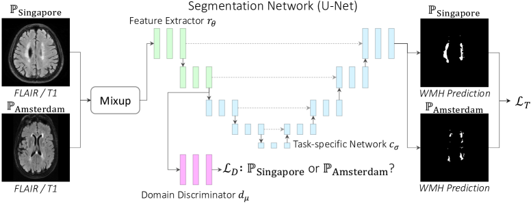
Fig. 1: MixDANN with Amsterdam and Singapore sources.

2.2 Mixup

Besides application of DANN, we also propose to use the common data-augmentation algorithm Mixup [12]. At first glance, this extension is fairly simple. Still, in the presence of multiple domains $\mathbb{P}_{1},\ldots,\mathbb{P}_{k}$, this algorithm complements the optimization objective in Eq. (1) because it also aims to produce domain invariance in our learning algorithm (discussed in the next sub-section). The algorithm is defined as follows. Suppose we have a batch of data-points $\{x_{i}\}_{i}$ with $x_{p}$ and $x_{q}$ two distinct data-points from this sample. Further, let $\lambda\sim\mathrm{Beta}(\alpha,\alpha)$. Then, we define the new mixed data-point:

$$\small\tilde{x}_{p,q}=\lambda x_{p}+(1-\lambda)x_{q}.$$ (3)

With a certain probability (e.g., 0.5 in all our experiments), we can then substitute every data-point in the batch $\{x_{i}\}_{i}$ with a mixed counterpart by randomly pairing the elements of $\{x_{i}\}_{i}$ and using Eq. (3) to combine them. We do remark that the original proposal for mixup also mixes across the label space. Our segmentation setting is slightly different due to the common use of a Dice score loss. Thus, we adopt a loss balancing strategy similar to [7]: $\mathcal{L}(\tilde{x}_{p,q})=\lambda\mathcal{L}^{p}(\tilde{x}_{p,q})+(1-\lambda)\mathcal{L}^{q}(\tilde{x}_{p,q})$ where $\mathcal{L}^{i}$ is the loss with the label $y_{i}$ of $x_{i}$.

2.3 Theoretical Motivations

DANN and the $\mathcal{H}$-divergence. While many works have used the motivation of domain invariant features for DG [8, 16], we note that the original theoretical motivation of DANN was based on the domain adaptation theory proposed by Ben-David et al. [14]. Recent extensions [8, 9, 17] build upon existing theory and algorithm to demonstrate justified applications of DANN in DG. Theoretically speaking, upper bounds on the error of the unseen target suggest we should minimize the $\mathcal{H}$-divergence – a measure of the difference between two domains. The objective described in Eq. (1) can be interpreted as minimizing the $\mathcal{H}$-divergence in a fairly formal sense because the $\mathcal{H}$-divergence measures a classifier’s ability to distinguish between domains. Motivated by this, we learn invariant features in Eq. (1) by maximizing the errors of the domain classifier $d_{\mu}$.

A Formal Discussion of Mixup. Mixup [12] is a special case of Vicinal Risk Minimization [18]. Usually, in machine learning, we use Empirical Risk Minimization which suggests estimating the true data-distribution by the empirical measure $P(x,y)=\frac{1}{n}\sum\nolimits_{i=1}^{n}\delta_{x_{i}}(x)\delta_{y_{i}}(y),$ with the Dirac measure $\delta_{*}$ estimating density at each data-point. In the more general case of Vicinal Risk Minimization, we allow freedom to use a density estimate in the vicinity of the data-point $x_{i}$ using the vicinal measure $v_{*}$ as $P_{v}(x,y)=\frac{1}{n}\sum\nolimits_{i=1}^{n}v_{x_{i}}(x)\delta_{y_{i}}(y)$. In Mixup, the modifications to our data described in Eq. (3) equate to sampling from a certain vicinal distribution $u_{*}$: $u_{x_{i}}(x)=\frac{1}{n}\sum\nolimits_{j=1}^{n}\mathbf{E}_{\lambda}\left[\delta_{\lambda x_{i}+(1-\lambda)x_{j}}(x)\right]$ where $\lambda\sim Beta$.

Algorithm 1 MixDANN for Domain Generalization

Data: Set of sample $x$ and label $y$ from Sources $\mathbb{P}_{1},\dots,\mathbb{P}_{k}$ and Target $\mathbb{Q}$
Models: U-Net (Feature Extractor $r_{\theta}$ and Task-specific Network $c_{\sigma}$), Domain Discriminator $d_{\mu}$

1:procedure Train MixDANN using Sources $(\mathbb{P}_{i})_{i}$

2:  for mini-batch of samples from sources $(x_{i})_{i}\sim(\mathbb{P}_{i})_{i}$ do

3:   Mixup: $\tilde{x}_{p,q}\leftarrow\lambda x_{p}+(1-\lambda)x_{q}$ for $p,q$ pairs, $\lambda\sim Beta(0.7,0.7)$

4:   Task Update: $\theta,\sigma\leftarrow\arg\min\nolimits_{\sigma,\theta}\sum\nolimits\mathcal{L}_{T}(\sigma,\theta,\tilde{x}_{i,j})$

5:   Domain Update: $\theta,\mu\leftarrow\arg\left[\min\nolimits_{\theta}\max\nolimits_{\mu}-\gamma\sum\nolimits\mathcal{L}_{D}(\mu,\theta,\tilde{x}_{i,j})\right]$

6:  end for

7:end procedure

8:procedure Testing MixDANN on Target $\mathbb{Q}$

9:  Prediction: $y_{i}\leftarrow c_{\sigma}\circ r_{\theta}(x_{i})$ for samples from target $x_{i}\sim\mathbb{Q}$

10:end procedure

Connecting Mixup to the $\mathcal{H}$-divergence. From the perspective of the mentioned theory motivating DANN for DG (above), this form of density estimation has interestingly been linked to invariant learning by data-augmentation [18]. In particular, the vicinal measure $v_{*}$ may be defined to promote learning which is invariant to features of our data (e.g., augmentation by noise seeks to make a neural network’s prediction invariant to noise in the input). By applying Mixup as defined in Eq. (3), we coincidentally mix features across the domains $\mathbb{P}_{1},\ldots,\mathbb{P}_{k}$ because $x_{p}$ and $x_{q}$ may be drawn from differing domains. In this sense, the proposed vicinal distribution $u_{*}$ estimates the density of a data point $x_{i}$ to promote invariance to domain features in our learning algorithm. Hence, Mixup in the presence of multiple domains may be viewed as a technique complementary to DANN. It too is aimed at training $r_{\theta}$ and $c_{\sigma}$ to be invariant to domain features so that the errors of the domain discriminator $d_{\mu}$ are maximized, and subsequently, the $\mathcal{H}$-divergence is minimized. Alg. 1 shows MixDANN, our algorithmic and theoretical combination of Mixup and DANN for DG.

3 Experiments

3.1 Experimental Setup

Datasets. We evaluate on two WMH datasets consisting of FLAIR (Fluid Attenuated Inverse Recovery), T1, and manual WMH segmentation for each subject: (1) a multi-site public MICCAI WMH Challenge Dataset [1] from three sites (Amsterdam (A), Singapore (S), Utrecht (U)) and (2) our local in-house dataset [19] from a single site (Pittsburgh (P)). See Fig. 2 for distinct scanners/protocols and [1, 19] for details.

Sites	$N$	Scanner	FLAIR Voxel Size (mm3)	TR/TE (ms)
Amsterdam	20	3T GE Signa HDxt	$0.98\times 0.98\times 1.20$	8000/126
Singapore	20	3T Siemens TrioTim	$1.00\times 1.00\times 3.00$	9000/82
Utrecht	20	3T Philips Achieva	$0.98\times 0.98\times 1.20$	11000/125
Pittsburgh	20	3T Siemens TrioTim	$1.00\times 1.00\times 3.00$	9160/90

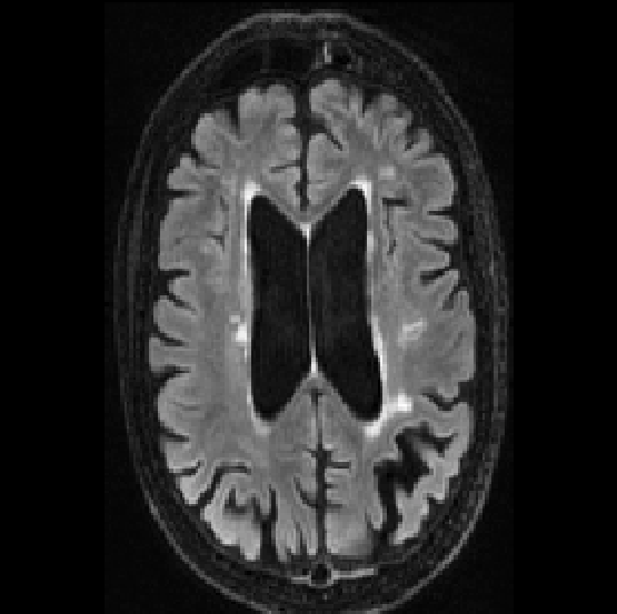
(a) Amsterdam

(b) Singapore

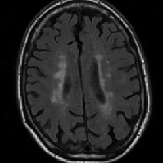
(c) Utrecht

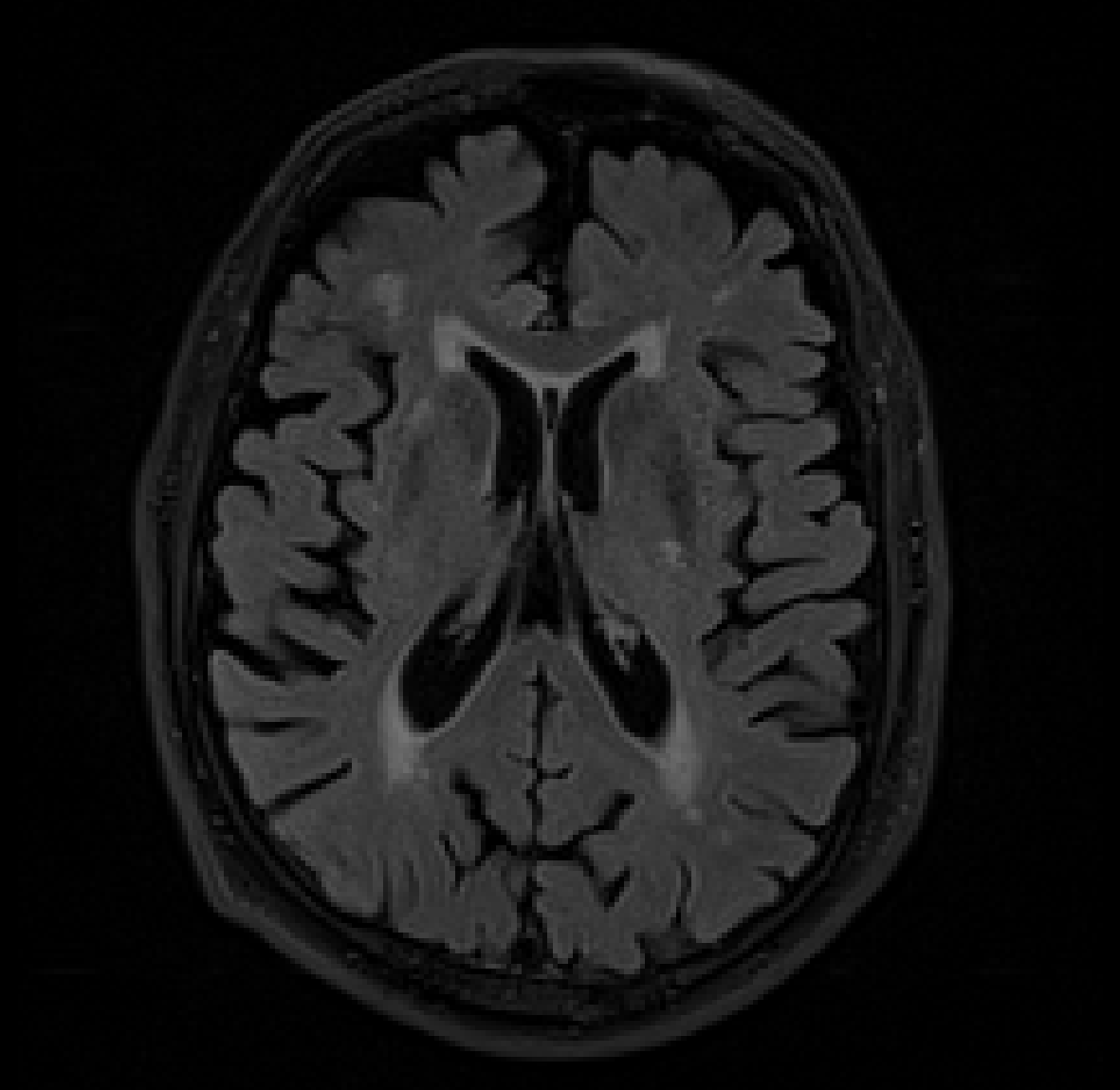
(d) Pittsburgh

Fig. 2: Top: Datasets with FLAIR and T1 (coregistered to FLAIR). Bottom: Sample FLAIR images.

Metrics. We use five evaluation metrics to assess the WMH prediction mask $\hat{Y}$ against the ground truth segmentation mask $Y$ (TP: true positive, FP: false positive, FN: false negative). (1) Dice Similarity Coefficient (DSC): $2(Y\cap\hat{Y})/(|Y|+|\hat{Y}|)$, (2) Housdorff Distance (H95): $H95=\max\{\sup\nolimits_{x\in Y}\inf\nolimits_{y\in\hat{Y}}d(x,y),\sup_{y\in Y}\inf_{x\in\hat{Y}}d(x,y)\}$ using the 95-th percentile distance, (3) Absolute Volume Difference (AVD) between the predicted and true WMH volume, (4) Lesion Recall: Computes the # of correctly detected WMH over the # of true WMH, (5) Lesion F1: TP / (TP + 0.5(FP+FN)).

Baseline Models. These baselines build on U-Net [20], and we report their results by a recent DA/DG work [4]: (1) DeepAll is the baseline U-Net with no DA or DG mechanisms which the following models build on. (2) UDA [4] is an unsupervised DA method using all target scans but not their labels. Note this DA method requires target thus has an advantage over DG methods. (3) BigAug [10] is a state-of-the-art DG medical imaging segmentation method with heavy data augmentations. See [4, 10] for full details.

Our Model. Our proposed approaches also build on U-Net. Standard data augmentations (rotation, scale, shear) are applied. (1) We implement our own DeepAll comparable to the DeepAll by [4] to our best effort for fair comparison. (2) DANN: We introduce the domain discriminator (Conv-Conv-Conv-FC-FC-FC) $d_{\mu}$ to U-Net to the output of the second downsampling layer (Fig. 1). For the purpose of DANN (Eq. (1)), we can treat the U-Net as $c_{\sigma}\circ r_{\theta}$ where $r_{\theta}$ is before and $c_{\sigma}$ is after the second downsampling. We slowly introduce $\mathcal{L}_{D}$ to $r_{\theta}$ by setting $\gamma=(2\cdot\xi)/(1+\exp(-\kappa\cdot p))-1$ in Eq. (1) with $p=\textrm{epoch}/\textrm{max\_epoch}$, $\kappa=3$, and $\xi=0.1$. (3) Mixup: We randomly mix the samples following Eq. (3) to induce domain invariance. (4) MixDANN: Our final model combines DANN and Mixup. The initial learning rate is 2e-4 for all models. We trained on 80% of the training data against the comparing methods using 2 x NVIDIA RTX2080Ti.

3.2 Results and Analysis

Each model tests on one target domain after training on the remaining sources (Sources$\rightarrow$Target). Generally, the comparison in DG is subjective across different experimental setups. For instance, despite the near identical architectures, our DeepAll slightly under-performs on some targets. As such, we pay special attention to the relative performance gain over the respective DeepAll to assess the domain generalizability.

Exp 1: DG within WMH Challenge Dataset. We test on each target by training on the remaining two sources. Table 1 shows the results of all targets and the average across them. We see that despite our weaker DeepAll, MixDANN shows the best absolute avg on three metrics (DSC, AVD, and Lesion F1) and the best relative gain on all metrics. We ablate and see improvements in the order of DANN, Mixup, and MixDANN, also visualized in Fig. 3. We note that AVD assessing the accuracy of the predicted WMH volume, which is often considered as a biomarker of vascular pathology, is most accurate by MixDANN. We also pay special attention to the improvement in the hardest case of A+S$\rightarrow$U: This exactly exemplifies a possible scenario where a DeepAll may fail on an unseen dataset but MixDANN can assure robustness.

Table 1: WMH Challenge Results. Sources$\rightarrow$Target: Trained on Sources and tested on Target among Amsterdam, Singapore, and Utrecht. avg: Average of the target results. gain: avg gain over the respective DeepAll.

Model	A+S$\rightarrow$U	U+S$\rightarrow$A	A+U$\rightarrow$S	avg	gain
DSC $\uparrow$ (Higher is better)
DeepAll ([4] Setup)	0.430	0.674	0.682	0.595	-
BigAug [10]	0.534	0.691	0.711	0.645	0.050
UDA [4] (Full Set)	0.529	0.737	0.782	0.683	0.087
DeepAll (Our Setup)	0.183	0.619	0.781	0.528	-
DANN	0.315	0.674	0.773	0.587	0.060
Mixup	0.619	0.691	0.835	0.715	0.187
MixDANN	0.694	0.700	0.839	0.744	0.217
H95 $\downarrow$ (Lower is better)
DeepAll	11.46	11.51	9.22	10.73	-
BigAug	9.49	9.77	8.25	9.17	-1.56
UDA (Full Set)	10.01	7.53	7.51	8.35	-2.38
DeepAll	42.69	18.05	4.56	21.77	-
DANN	38.56	15.48	5.15	19.73	-2.03
Mixup	24.08	13.21	5.70	14.33	-7.44
MixDANN	20.57	12.75	3.10	12.14	-9.63
AVD $\downarrow$ (Lower is better)
DeepAll	54.84	37.60	45.95	46.13	-
BigAug	47.46	30.64	35.41	37.84	-8.29
UDA (Full Set)	54.95	30.97	22.14	36.02	-10.11
DeepAll	384.19	43.28	23.26	150.24	-
DANN	134.03	26.65	24.09	61.59	-88.66
Mixup	42.09	33.47	13.41	29.66	-120.59
MixDANN	23.40	26.48	12.81	20.89	-129.35
Lesion Recall $\uparrow$ (Higher is better)
DeepAll	0.634	0.692	0.641	0.656	-
BigAug	0.643	0.709	0.691	0.681	0.025
UDA (Full Set)	0.652	0.841	0.754	0.749	0.093
DeepAll	0.309	0.623	0.705	0.546	-
DANN	0.349	0.630	0.740	0.573	0.028
Mixup	0.556	0.700	0.790	0.682	0.136
MixDANN	0.604	0.685	0.797	0.695	0.150
Lesion F1 $\uparrow$ (Higher is better)
DeepAll	0.561	0.673	0.592	0.609	-
BigAug	0.577	0.704	0.651	0.644	0.035
UDA (Full Set)	0.546	0.739	0.649	0.645	0.036
DeepAll	0.288	0.554	0.697	0.513	-
DANN	0.309	0.610	0.708	0.542	0.029
Mixup	0.515	0.642	0.724	0.627	0.114
MixDANN	0.602	0.651	0.728	0.660	0.147

Table 2: WMH Segmentation Results of A+S+U$\rightarrow$Pitt

Model	DSC $\uparrow$	H95 $\downarrow$	AVD $\downarrow$	Recall $\uparrow$	F1 $\uparrow$
DeepAll	0.434	18.49	68.56	0.543	0.630
DANN	0.499	16.04	62.31	0.622	0.680
Mixup	0.462	16.92	65.92	0.501	0.606
MixDANN	0.488	15.93	63.41	0.466	0.566

Exp 2: A+S+U$\rightarrow$Pitt. We do a “cross-dataset” DG: train on A+S+U and test on Pitt. We could not include Pitt as a source since it only has 5 consecutive slices of manual segmentation available. Nonetheless, when we test it as a target as shown in Table 2, we again see consistent improvements over DeepAll. Interestingly, DANN best performs, implying that Mixup and DANN may also individually bring benefits. Our MixDANN with a single U-Net is now ranked 6^th on the leader board of the WMH Challenge [1], competitive against other top ensemble U-Nets. We observe poor performance by Mixup on the WMH counting metrics (Recall and F1), suspecting this to be from the different manual annotation standards between the two datasets. We consider this as our future work.

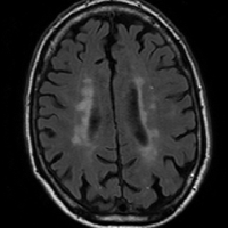
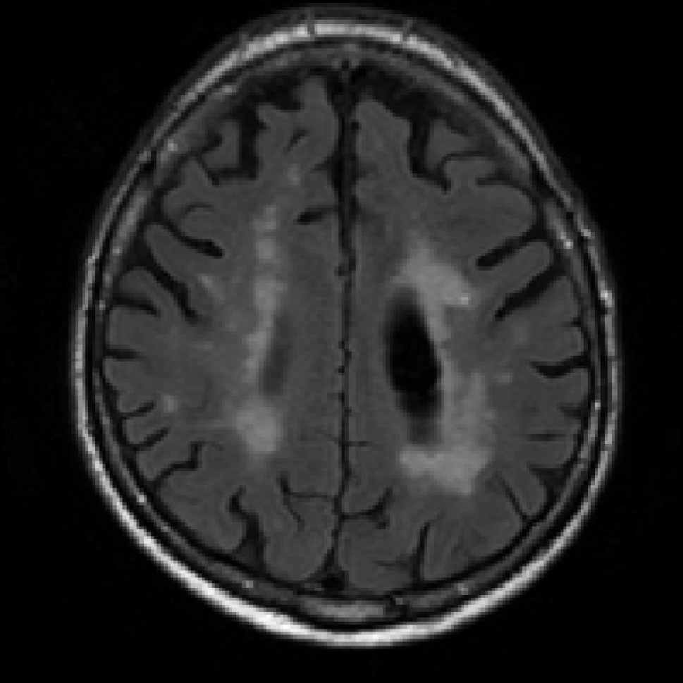
(a) FLAIR

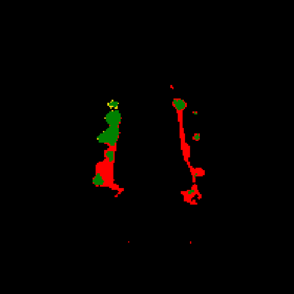
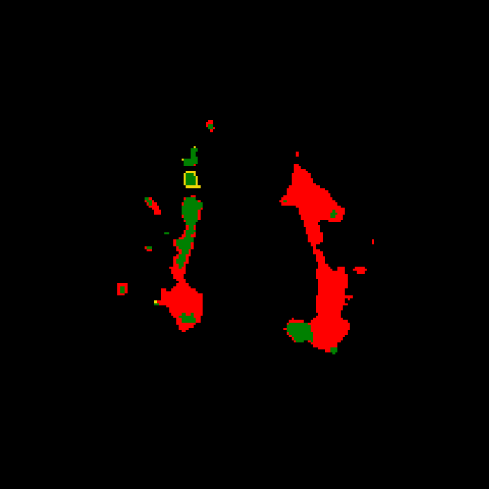
(b) DeepAll

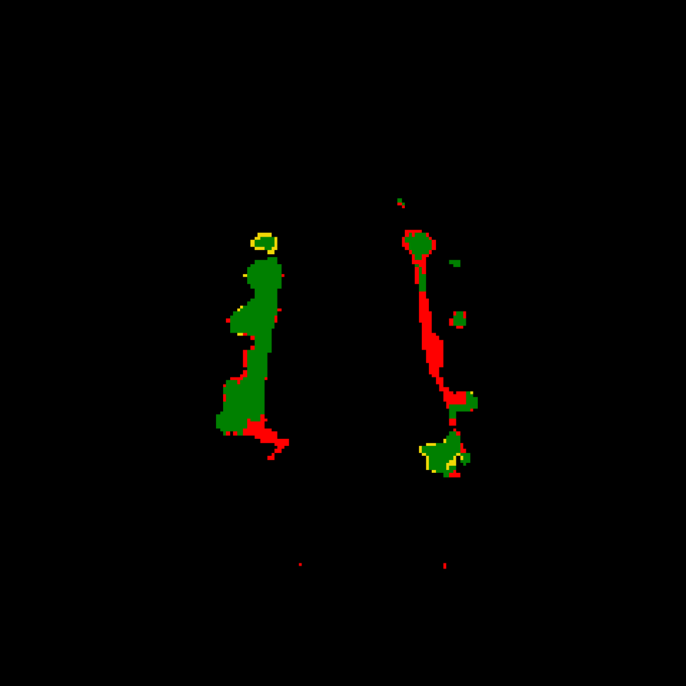
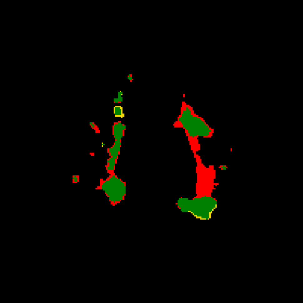
(c) DANN

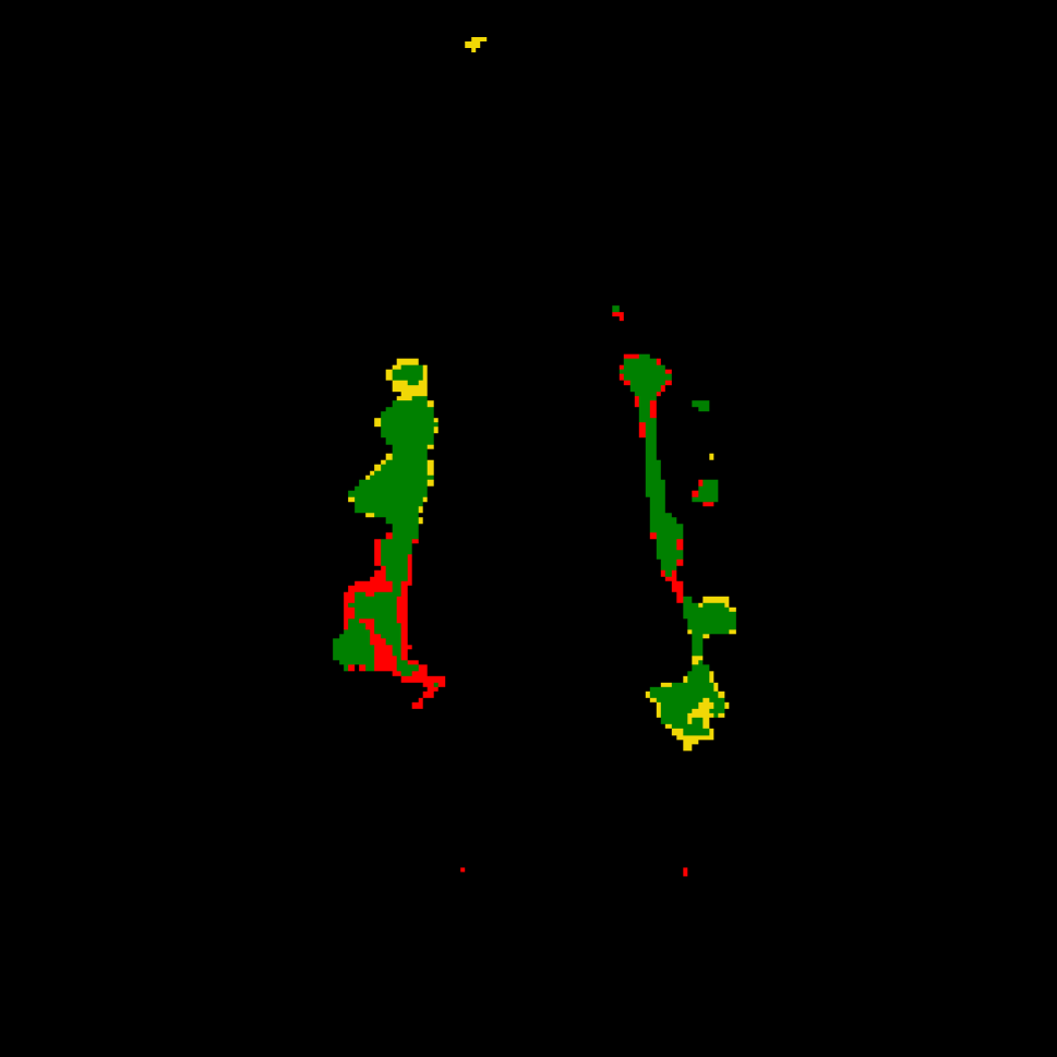
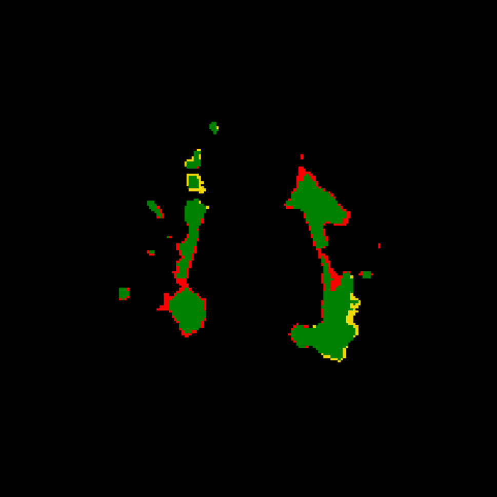
(d) Mixup

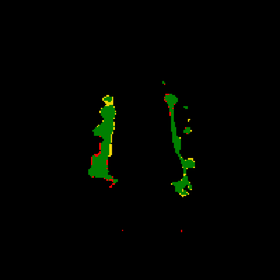
(e) MixDANN

Fig. 3: Visualization of WMH predictions (A+S$\rightarrow$U). True Positive: Green, False Positive: Yellow, False Negative: Red.

Do we learn domain-invariance? Fig. 4 shows the t-SNE [21] plots of the second downsampling layer ($r_{\theta}$) output. We see that the features by DeepAll can easily identify certain domains while those by MixDANN blur the boundary among domains as intended. In the context of WMH prediction, MixDANN explicitly suppresses the site/scanner dependent information, thus is more robust when test on unseen data.

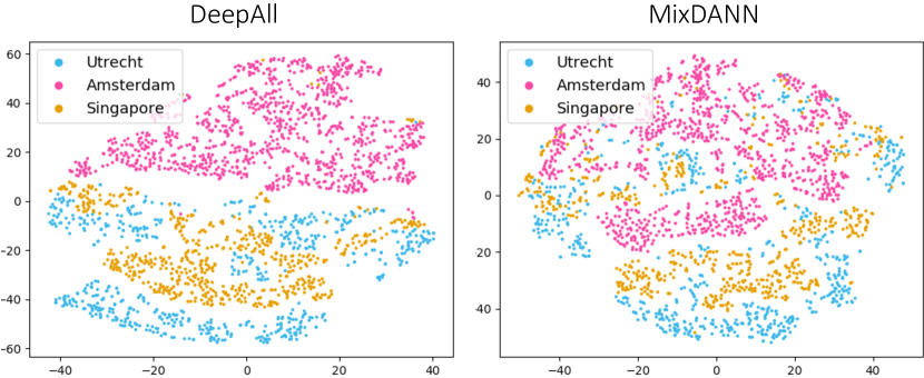
Fig. 4: t-SNE plots of U-Net features trained on Amsterdam (pink), Singapore (gold) and Utrecht (blue) as sources.

4 Conclusion

We investigate the domain generalizability of a WMH segmentation deep model to be trained on sources and operate well on an unseen target. We identify a theoretical connection between two DG approaches, namely DANN and Mixup, and jointly incorporate them into U-Net. Using a multi-site WMH dataset and our local dataset, we show our domain invariant learning frameworks bring drastic improvements over other DA/DG methods in both relative and absolute performances.

5 Acknowledgments

This work was supported by the NIH/NIA (R01 AG063752, RF1 AG025516, P01 AG025204, K23 MH118070), and SCI UR Scholars Award. We report no conflicts of interests.

6 Compliance with Ethical Standards

The WMH Challenge study was conducted retrospectively using open access data by WMH Segmentation Challenge (https://wmh.isi.uu.nl/). Ethical approval was not required as confirmed by its license. The Pitt study performed in line with the principles of the Declaration of Helsinki was approved by the Ethics Committee of the University of Pittsburgh.

References

- [1] Hugo J Kuijf, J Matthijs Biesbroek, Jeroen De Bresser, Rutger Heinen, Simon Andermatt, Mariana Bento, Matt Berseth, Mikhail Belyaev, M Jorge Cardoso, Adria Casamitjana, et al., “Standardized Assessment of Automatic Segmentation of White Matter Hyperintensities and Results of the WMH Segmentation Challenge,” IEEE TMI, vol. 38, no. 11, pp. 2556–2568, 2019.
- [2] Ben Glocker, Robert Robinson, Daniel C Castro, Qi Dou, and Ender Konukoglu, “Machine learning with multi-site imaging data: An empirical study on the impact of scanner effects,” arXiv preprint arXiv:1910.04597, 2019.
- [3] Hoo-Chang Shin, Holger R Roth, Mingchen Gao, Le Lu, Ziyue Xu, Isabella Nogues, Jianhua Yao, Daniel Mollura, and Ronald M Summers, “Deep convolutional neural networks for computer-aided detection: CNN architectures, dataset characteristics and transfer learning,” IEEE TMI, vol. 35, no. 5, pp. 1285–1298, 2016.
- [4] Hongwei Li, Timo Loehr, Anjany Sekuboyina, Jianguo Zhang, Benedikt Wiestler, and Bjoern Menze, “Domain Adaptive Medical Image Segmentation via Adversarial Learning of Disease-Specific Spatial Patterns,” 2020.
- [5] Yaroslav Ganin and Victor Lempitsky, “Unsupervised Domain Adaptation by Backpropagation,” in ICML, 2015.
- [6] Cian M Scannell, Amedeo Chiribiri, and Mitko Veta, “Domain-Adversarial Learning for Multi-Centre, Multi-Vendor, and Multi-Disease Cardiac MR Image Segmentation,” arXiv preprint arXiv:2008.11776, 2020.
- [7] Egor Panfilov, Aleksei Tiulpin, Stefan Klein, Miika T Nieminen, and Simo Saarakkala, “Improving robustness of deep learning based knee mri segmentation: Mixup and adversarial domain adaptation,” in ICCV Workshop, 2019.
- [8] Toshihiko Matsuura and Tatsuya Harada, “Domain Generalization Using a Mixture of Multiple Latent Domains,” in AAAI, 2020.
- [9] Anthony Sicilia, Xingchen Zhao, and Seong Jae Hwang, “Domain adversarial neural networks for domain generalization: When it works and how to improve,” arXiv preprint arXiv:2102.03924, 2021.
- [10] Ling Zhang, Xiaosong Wang, Dong Yang, Thomas Sanford, Stephanie Harmon, Baris Turkbey, Bradford J Wood, Holger Roth, Andriy Myronenko, Daguang Xu, et al., “Generalizing deep learning for medical image segmentation to unseen domains via deep stacked transformation,” IEEE TMI, 2020.
- [11] Pulkit Khandelwal and Paul Yushkevich, “Domain Generalizer: A Few-Shot Meta Learning Framework for Domain Generalization in Medical Imaging,” in MICCAI Workshop on DART/DCL. Springer, 2020.
- [12] Hongyi Zhang, Moustapha Cisse, Yann N Dauphin, and David Lopez-Paz, “mixup: Beyond Empirical Risk Minimization,” in ICLR, 2018.
- [13] Shai Ben-David, John Blitzer, Koby Crammer, and Fernando Pereira, “Analysis of representations for domain adaptation,” in Neurips, 2007.
- [14] Shai Ben-David, John Blitzer, Koby Crammer, Alex Kulesza, Fernando Pereira, and Jennifer Wortman Vaughan, “A theory of learning from different domains,” Machine learning, vol. 79, no. 1-2, pp. 151–175, 2010.
- [15] Boris Shirokikh, Ivan Zakazov, Alexey Chernyavskiy, Irina Fedulova, and Mikhail Belyaev, “First U-Net Layers Contain More Domain Specific Information Than The Last Ones,” in MICCAI Workshop on DART/DCL. Springer, 2020.
- [16] Haoliang Li, Sinno Jialin Pan, Shiqi Wang, and Alex C Kot, “Domain generalization with adversarial feature learning,” in CVPR, 2018.
- [17] Isabela Albuquerque, João Monteiro, Tiago H Falk, and Ioannis Mitliagkas, “Generalizing to unseen domains via distribution matching,” arXiv preprint arXiv:1911.00804, 2020.
- [18] Olivier Chapelle, Jason Weston, Léon Bottou, and Vladimir Vapnik, “Vicinal risk minimization,” in Neurips, 2001.
- [19] Helmet T Karim, Dana L Tudorascu, Ann Cohen, Julie C Price, Brian Lopresti, Chester Mathis, William Klunk, Beth E Snitz, and Howard J Aizenstein, “Relationships between executive control circuit activity, amyloid burden, and education in cognitively healthy older adults,” Am. J. Geriatr. Psychiatry, vol. 27, 2019.
- [20] Olaf Ronneberger, Philipp Fischer, and Thomas Brox, “U-net: Convolutional networks for biomedical image segmentation,” in MICCAI. Springer, 2015.
- [21] Laurens van der Maaten and Geoffrey Hinton, “Visualizing data using t-sne,” JMLR, vol. 9, 2008.