The EDGE-CALIFA survey: The local and global relations between $\Sigma_{\rm*}$ , $\Sigma_{\rm SFR}$ and $\Sigma_{\rm mol}$ that regulate star-formation

Abstract

We present a new characterization of the relations between star-formation rate, stellar mass and molecular gas mass surface densities at different spatial scales across galaxies (from galaxy wide to kpc-scales). To do so we make use of the largest sample combining spatially-resolved spectroscopic information with CO observations, provided by the EDGE-CALIFA survey, together with new single dish CO observations obtained by APEX. We show that those relations are the same at the different explored scales, sharing the same distributions for the explored data, with similar slope, intercept and scatter (when characterized by a simple power-law). From this analysis, we propose that these relations are the projection of a single relation between the three properties that follows a distribution well described by a line in the three-dimension parameter space. Finally, we show that observed secondary relations between the residuals and the considered parameters are fully explained by the correlation between the uncertainties, and therefore have no physical origin. We discuss these results in the context of the hypothesis of self-regulation of the star-formation process.

1 Introduction

Star-formation is likely the central physical process defining the nature and evolution of galaxies. Indeed, gas clouds trapped in dark-matter halos not forming stars are considered as failed galaxies (e.g. Whitmore, 1992). This process requires very particular physical conditions that allow first, the formation of molecular clouds from the more diffuse atomic gas content (mostly HI), and second the fragmentation of those clouds that collapse in order to reach the densities (and temperatures) required to ignite the thermonuclear reactions that define stars. Star-forming galaxies, i.e., those that actively form stars across their optical extent, follow three well known scaling relations between their global star-formation rate, gas mass, and stellar mass content, whose nature is still not fully understood.

The relation between the star-formation rate (SFR) and the cold gas mass ( atomic and molecular) is known as the Schmidt-Kennicutt law (SK-law, or simply, the star-formation-law or SF-law). It was first proposed by Schmidt (1959) as a relation between the SFR and the mass of cold gas in a certain volume, with the form of a simple power-law, based on purely theoretical considerations. He estimates the slope of this power-law between 2-3, based on the comparison between the dispersion in the vertical direction of our galaxy of both the neutral hydrogen and the number of young stars. The SK-law was empirically confirmed as a relation between the average SFR and cold gas surface densities, atomic plus molecular, averaged over the optical extent of galaxies. Thus, this is a relation between two intensive quantities ($\Sigma_{\rm SFR}$ and $\Sigma_{\rm gas}$ ), i.e., quantities that do not depend on the size of galaxies. A initial slope of 1.3$\pm$0.3 was found by Kennicutt (1989), with values between 0.9-1.7 reported in subsequent studies using different estimations of the SFR and the cold gas content (as reviewed in Kennicutt, 1998a).A simple free-fall timescale argument was proposed by this author to explain this relation, and the value of its exponent. Based on a compilation of literature data Kennicutt (1998a) proposed a relation with slope of 1.4$\pm$0.15, and a dispersion of $\sim$0.28 dex, in $\Sigma_{\rm SFR}$ , using the total cold gas density (i.e., $\Sigma_{\rm gas}$ ). A similar relation has been found to hold not only galaxy wide, but also at local/resolved scales (down to $\sim$500 pc), but only when using the molecular gas surface density (i.e., $\Sigma_{\rm mol}$ ). This relation, known as resolved Schmidt-Kennicutt law or rSK-law, presents a slope slightly lower or near to $\sim$1 and a dispersion of the order of $\sim$0.2 dex in $\Sigma_{\rm SFR}$ (e.g Wong & Blitz, 2002; Kennicutt et al., 2007; Bigiel et al., 2008; Leroy et al., 2013), as recently reviewed in Sánchez (2020).

Large galaxy spectroscopic and imaging surveys like the Sloan Digital Sky Survey (SDSS, York et al., 2000), reveal a tight relation between the integrated SFR and stellar mass in galaxies, known as the star-formation main sequence (SFMS, e.g. Brinchmann et al., 2004; Renzini & Peng, 2015). Like the SK-law, this relation follows a power-law, with a power/slope near or slightly lower than $\sim$1 at z$\sim$0. However, contrary to the SK-law, it is well documented that the SFMS evolves with time (e.g. Speagle et al., 2014; Rodríguez-Puebla et al., 2016), as galaxies become less massive (in stellar mass) and exhibit larger SFR following the cosmological increase in SFR density (e.g. Madau & Dickinson, 2014; Sánchez et al., 2019a). The zero-point of the relation is essentially constant in the nearby Universe ($z<$0.15), followed by a strong increase from $z\sim$0.2 to $z\sim$2. The slope presents a similar trend, but with a weaker or no evolution, depending on the authors (e.g, Fig. 7 and 8 from Sánchez et al., 2019a). In contrast with the SK-law, the SFMS was first expressed as a relation between extensive quantities (integrated M_∗ and SFR), i.e., between parameters which value depends on the size of galaxies. Sánchez et al. (2013) and Wuyts et al. (2013) first reported a similar relation between the SFR and M_∗ surface densities of star-forming regions within galaxies found at kpc-scales (i.e., $\Sigma_{\rm SFR}$ vs. $\Sigma_{\rm*}$ ). This relation between intensive quantities, known as the resolved SFMS (or rSMFS), was explored in detail by Cano-Díaz et al. (2016a), using a sample of galaxies with spatial resolved spectroscopic information extracted from the Calar Alto Legacy Integral Field Area (CALIFA) integral-field spectroscopy (IFS) survey (Sánchez et al., 2012). They found that this relation presents a similar shape at a kpc-scale as the global one and a similar scatter ($\sim$0.25 dex). A possible morphological dependence of the shape of the global and local/resolved SFMS relations has been reported in different studies (e.g. González Delgado et al., 2016; Catalán-Torrecilla et al., 2017; Cano-Díaz et al., 2019). More recently, the decomposition between the disk and bulge components in galaxies has shown that the reported differences by morphological types may be artificial: Méndez-Abreu et al. (2019) showed that the SFMS relations for the disk component of both late- and early-type galaxies are statistically indistinguishable, despite the fact that a clear difference is appreciated if the integrated quantities (disk+bulge) are adopted. In summary, the disks of galaxies with different morphologies present the same SFMS relations.

Finally, a similar relationship has been described between the molecular gas and stellar masses in SF galaxies (e.g. Saintonge et al., 2016; Calette et al., 2018). This relation, known now as the Molecular Gas Main Sequence (MGMS), has not been explored as much as the previous two. In its spatially resolved form it was only recently described as a power-law relation between the surface densities of both quantities by Lin et al. (2019) (e.g. $\Sigma_{\rm mol}$ vs. $\Sigma_{\rm*}$ ). In that study, the authors used a limited sample of just 14 galaxies extracted from the MaNGA (Bundy et al., 2015a) IFS survey, observed with the Atacama Large Millimeter Array (ALMA) to provide kpc-scale CO-mapping (as part of the ALMaQUEST compilation Lin et al., 2020). They found that this relation exhibits a slope $\sim$1 and a scatter of $\sim$0.2 dex (the so-called rMGMS relation). A more recent exploration by Ellison et al. (2020a), increasing the number of studied ALMaQUEST galaxies by a factor two, provided a similar result.

The connection between the global and local/resolved versions of the three relations has been a topic of study in different studies. Bolatto et al. (2017) first showed that a simple parametrization describing the global intensive SK-law follows the observed trend of the local/resolved distribution of the two considered parameters. In the case of the SFMS, the correspondence between the global and local/resolved relations was first explored by Pan et al. (2018) and Cano-Díaz et al. (2019). More recently, Sánchez et al. (2020), using a large compilation of galaxies observed using IFS at kpc-scales ($\sim$8,000 galaxies), and an indirect proxy for the molecular gas, demonstrated that the global and local/resolved versions of the MGMS follow similar distributions, when the global relation is presented in its intensive form (i.e., the average surface density across the optical extent of galaxies, following Cano-Díaz et al., 2019).

The nature of the scatter described in the three relations and the existence of possible secondary relations with other parameters, that may drive this scatter, is an important topic of study. Whether the morphology, the gas content, the star-formation efficiency (SFE) , or any other property still not explored in the literature modulate the relation between the three parameters is of a key importance to understand the processes that regulate SF in galaxies (and regions within galaxies). As indicated before, early results suggest that the SFMS may depend on the morphology (Catalán-Torrecilla et al., 2017). However, the results were not totally conclusive. Some hints of dependence was reported for the rSFMS (e.g. Cano-Díaz et al., 2019) with the morphology, while clear variations were reported by more recent explorations (Ellison et al., 2020a). Finally, it has not been explored if these differences in the rSFMS are induced by the presence of the bulge, like it was found by Méndez-Abreu et al. (2019) for the integrated/global SFMS relation (as quoted before). On the other hand, it is known that as star-formation halts/quenches in galaxies (and regions within galaxies), they depart from the explored relations, with the gas fraction ($f_{gas}$) being the major driver of this separation (e.g. Saintonge et al., 2016; Calette et al., 2018; Colombo et al., 2018; Sánchez et al., 2018; Sánchez et al., 2020; Colombo et al., 2020). Although the separation from the three relations traced by retired galaxies is directly related to a lack of (molecular) gas, the dispersion within the rSFMS (i.e., among SFGs) was reported to depend both on the SFE and the gas fraction (Ellison et al., 2020d; Colombo et al., 2020; Ellison et al., 2020a). The relative importance of both parameters is still unclear in driving this dispersion, although the SFE seems to out-rank the gas fraction(Ellison et al., 2020d, , Fig. 4). The presence of additional parameters that modulate these relations may indicate the existence of a generalized star-formation law from which the observed ones are just projections in a more limited space of parameters (e.g. Shi et al., 2018; Dey et al., 2019; Barrera-Ballesteros et al., 2021a). On the other hand, the need of additional parameters may indicate the existence of a so-far hidden parameter that regulates the three relations (e.g., the gas pressure Barrera-Ballesteros et al., 2021b)

In this article we attempt to characterize the three relations in their global intensive and local/resolved forms using a large and statistically significant sample of galaxies observed using both IFS and resolved and aperture limited molecular gas mapping. To do so we use the extended CALIFA sample (Sánchez et al., 2012), in combination with the recent single dish CO-mapping provided by APEX (Colombo et al., 2020) and the spatially resolved CO-mapping provided by the EDGE survey (Bolatto et al., 2017). This compilation comprises the largest available dataset of the three considered parameters, including estimations covering the entire galaxies (CALIFA), aperture limited (APEX), and spatially resolved (at kpc-scales, EDGE). The three datasets have different spatial resolutions and they cover different regimes of the same galaxies (or a subset of them). We will treat them separately to narrow-down the effects of resolution and apertures in the explored relations, comparing the results derived from each of them when needed. In addition we explore the correspondence between the global intensive and local/resolved relations. Particular care has been taken in the interpretation of possible secondary relations and the effects of errors, which has not been addressed in detail before. The structure of this articles is as follows: the galaxy samples and adopted datasets are described in Sec. 2, with details of the optically derived parameters included in Sec. 2.1 and the CO-derived ones in Sec. 2.2; a summary of the main properties of the different galaxy subsamples, compared with the ones adopted by previous explorations, is presented in Sec. 2.3; the analysis performed on the data is described in Sec. 3, with a description of the possible secondary relations included in Sec. 3.3; the effects of errors in the apparent generation of these relations are described in Sec. 3.4. Finally, we present the main conclusions and a discussion of the results in Sec. 4.

Throughout this article we assume the standard $\Lambda$ Cold Dark Matter cosmology with the parameters: $H_{0}$=71 km/s/Mpc, $\Omega_{M}$=0.27, $\Omega_{\Lambda}$=0.73.

2 Sample and data

The galaxies explored in this study were extracted from the extended CALIFA sample (eCALIFA, Espinosa-Ponce et al., 2020; Lacerda et al., 2020). The Calar Alto Legacy Integral Field Area survey (Sánchez et al., 2012) is a survey of galaxies in the nearby universe ($z<0.1$), observed at the 3.5m telescope of the Calar Alto observatory, using the PPAK (Kelz et al., 2006) wide Integral Field Unit of the PMAS (Roth et al., 2005) spectrograph. PPAK offered one of the largest Field-of-views of currently existing IFUs (74$\arcsec$$\times$64$\arcsec$), sampled with a $\sim$60% covering factor by 2.7$\arcsec$ fibers. Adopting a three dithering observing scheme (i.e., three pointings with an offset smaller than the distance between fibers) the complete Field-of-View (FoV) is sampled, providing a final point-spread-function (PSF) full-width at half-maximum (FWHM) of $\sim$2.5$\arcsec$ (García-Benito et al., 2015a). Two observational setups were adopted: the intermediate resolution V1200 setup (3700-4800Å, $\lambda/\Delta\lambda\sim$1650) and the low resolution V500 setup (3745-7500 Å, $\lambda/\Delta\lambda\sim$850); the latter in the one used in this study.

Galaxies were diameter-selected to match their optical extent with the FoV of the IFU, covering up to 2.5 effective radius in all the galaxies (Walcher et al., 2014). Additional cuts were imposed on the original mother sample to exclude dwarf galaxies and extremely massive ones. As explained in Sánchez et al. (2012) and Walcher et al. (2014) in detail, dwarfs (M$<$10⁷M_⊙) were originally excluded since their evolution is known to be different than more massive galaxies (M$>$10^8.5M_⊙), and they would dominate the number of objects if a pure diameter selection is performed (as they are far more numerous). On the other hand, extremelly massive galaxies are very rare in number in the nearby universe and for the covered volume no representative sample could be selected impossing a diameter selection. The cuts guarantee the statistical significance of the CALIFA mother sample.

At the completion of the CALIFA survey, a set of subsamples were observed to increase the number of certain galaxy types either excluded due to the cuts indicated before (dwarfs, large ellipticals) or resulting in low numbers in the final sample, or additional galaxies of particular interest (like hosts of recent supernovae). These extended samples fulfill the main selection criteria of the original sample (low-redshift, diameter selection), increasing the number statistics. All of them were observed using the same instrumental setup, with the same observing strategy and reduced and analyzed in a similar way. A particularly large number of galaxies in these extended samples ($\sim$100) correspond to ongoing SN host exploration by the PMAS/PPak Integral-field Supernova Hosts Compilation (PISCO Galbany et al., 2018). As discussed in Sánchez et al. (2016c), all these galaxies where included in the CALIFA database, as a set of extended subsamples.

All together, the final extended CALIFA sample (Espinosa-Ponce et al., 2020; Lacerda et al., 2020) comprises, so far, 941 galaxies with good quality observations using the V500 setup. All data were reduced using version 2.2 of the CALIFA pipeline (Sánchez et al., 2016c), that performs all the usual reduction steps for fiber-fed integral field spectroscopy (Sánchez, 2006), including fiber tracing, extraction, wavelength calibration, fiber-to-fiber corrections, flux calibration and spatial registration. The final product of the data-reduction is a cube with the spatial information registered in the x and y axis, and the spectral one in the z axis . The final reconstructed datacube has a sampling of 1$\arcsec$ per spaxel, large enough to correctly sample the final PSF (according to the Nyquist–Shannon sampling theorem, Nyquist, 1928; Shannon, 1948), without a large oversampling (and the corresponding increase of the co-variance). The final datacubes have an astrometry accuracy of $\sim$0.5$\arcsec$, an absolute photometric calibration precision of $\sim$8% ( and a $\sim$5% relative from blue to red, what quantifies the color effect in the spectra), and a depth of $r\sim$23.6 mag/arcsec². Details on the data reduction and the quality of the data can be found in Sánchez et al. (2012); Husemann et al. (2013); García-Benito et al. (2015b); Sánchez et al. (2016c).

2.1 Optical derived parameters

The IFS data provided by the CALIFA observations are analyzed using the Pipe3D dedicated pipeline (Sánchez et al., 2016a, b), to extract the most relevant physical parameters of the stellar population (luminosity weighted ages and metallicities, dust attenuation, light distribution by ages, stellar velocity and velocity dispersion…) and emission lines (line fluxes, equivalent widths, ionized gas velocity and velocity dispersion…) . Details of this pipeline, explanations regarding the derivations of the different parameters, reliability tests, and examples of its use have been extensively given in many different articles (e.g. Cano-Díaz et al., 2016a; Ibarra-Medel et al., 2019; Bluck et al., 2019; Ellison et al., 2020d; Lacerda et al., 2020; Sánchez, 2020, for citing just a few). In summary, the pipeline performs an analysis of the stellar population and emission line properties by modelling each spectrum in the cube with a combination of a set of single-stellar populations models (SSPs), using a particular stellar library, and a set of Gaussian functions to describe the emission lines. Stellar population models are convolved with a line-of-sight velocity distribution to recover the stellar kinematics, while the gas kinematics are recovered by the Gaussian fitting itself. The stellar dust attenuation is derived in an iterative procedure, using the same optical spectra. The procedure involves spatially binning the data to increase the signal-to-noise above a threshold of $\sim$50 at which the stellar population analysis provides with reliable results based on simulations (Sánchez et al., 2016b), and a dezonification to recover a model for the original sampled spaxels (Cid Fernandes et al., 2013). In addition to this modelling, the stellar-subtracted datacube (the so-called gas-pure cube) is analyzed based on a moment analysis to recover the properties of the emission lines in more detail (i.e., flux intensity, equivalent width, velocity and velocity dispersion). The Pipe3D pipeline was developed to analyse IFS data of different origin, and has been tested with CALIFA (e.g. Cano-Díaz et al., 2016a; Sánchez et al., 2017), MaNGA (e.g. Ibarra-Medel et al., 2016; Cano-Díaz et al., 2019; Lin et al., 2019), SAMI (e.g. Sánchez et al., 2019b) and MUSE data (e.g. López-Cobá et al., 2020).

The most relevant parameters for the current study derived based on the Pipe3D analysis are: (i) the stellar mass; (ii) the star-formation rate and (iii) a proxy for the molecular gas that will be explained in detail below. All these three quantities are derived both integrated across the FoV of the IFS data and spatially resolved, spaxel-to-spaxel, as surface densities. We summarise here how these quantities are derived. For a more detailed explanation, we refer the reader to Sánchez et al. (2020), in which the derivation is explained in more detail:

Stellar mass (M_∗): It is derived from the multi-SSP decomposition of the stellar population, spaxel-by-spaxels, performed by the pipeline (Sánchez et al., 2016a). This procedure provides the mass-to-light ratio (M/L) at each spaxel, estimated as the average of the M/L of each SSP weighted by the relative contribution in light of each one to the total observed spectrum. Multiplying this M/L by the luminosity in each spaxel at the considered band (in our case the $V$-band), considering the observed flux intensity, correcting by the cosmological distance, and the stellar dust attenuation we obtain the stellar mass within each spaxel across the datacube. Then, the integrated stellar mass is derived by co-adding these individual values for each spaxel, while the stellar mass surface density ($\Sigma_{\rm*}$ ) is derived by dividing the stellar mass within each spaxel by the area in physical quantities (pc², in our case). For the current implementation of the analysis we adopted a Salpeter (1955) Initial Mass Function (IMF) with the standard limits in stars masses (0.1-100 M_⊙). The errors in the derivation of the stellar masses are dominated by a combination of photometric calibration errors in the optical data ($\sim$0.05 dex Sánchez et al., 2016c), and the intrinsic uncertainties in the derivation of this quantity by the adopted method ($\sim$0.1 dex Sánchez et al., 2016a), rather than the statistical photon noise (that is more or less homogenized due to adopted spatial binning procedure). When adding this later error the typical uncertainty for $\Sigma_{\rm*}$ is of the order of $\sim$0.15 dex.

Star-formation rate (SFR): The SFR is derived spaxel-by-spaxel using the scaling relation proposed by Kennicutt et al. (1989) between this quantity and the H$\alpha$ luminosity, SFR[M_⊙/yr]$=8\times 10^{-42}$ L_Hα[erg/sec] (again, adopting a Salpeter IMF), for those spaxels compatible with being ionized by young OB stars, i.e., tracing star-formation (SF). To determine which spaxels are dominated by ionization by young stars , we use the information provided by moment analysis of the emission lines, in particular the emission line intensities of the $\rm{H}\alpha$, $\rm{H}\beta$, [O iii] $\lambda$5007,$\lambda$4959 and [N ii] $\lambda$6548,$\lambda$6584. We adopted the ionizing classification scheme proposed in (Sánchez, 2020), in which a spaxel is consider to be ionized by SF if it is located below the (Kewley et al., 2001) demarcation line in the classical BPT diagnostic diagram (i.e., the one involving the [O iii]/$\rm{H}\beta$ vs [N ii]/$\rm{H}\alpha$ line ratio Baldwin et al., 1981) and it has an EW(H$\alpha$)$>$6Å. Then the H$\alpha$ luminosity is derived based on the observed flux intensity, correcting by the cosmological distance, and the interstellar medium dust attenuation (derived from the $\rm{H}\alpha$/$\rm{H}\beta$ line ratio, assuming a Cardelli et al., 1989, extinction law). Finally, using the scaling relation outlined before and co-adding across the FoV of the instrument, we derive the integrated SFR. Following Sánchez et al. (2020), no signal-to-noise cut was applied to the emission lines along this process, since this could bias the results, in particular for the detection of low-intensity and low-EW diffuse ionized regions. We rather prefer to propagate the errors. However, for the SF-regions, the combined requirement of a large EW(H$\alpha$) and a physically reliable dust attenuation, impose an implicit S/N in H$\alpha$ well above 3$\sigma$. Dividing the derived SFR by the area in each spaxel yields the SFR surface density ($\Sigma_{\rm SFR}$ ). Like in the case of the stellar masses, the individual errors were derived propagating both the statistical errors (errors in the derivation of H$\alpha$ and the dust attenuation) and the photometric calibration ones. The typical error is of the order of $\sim$0.10 dex for the full sample.

Molecular gas mass (M_mol): We do not have a spatial or integrated estimation of the molecular gas content for the entire CALIFA sample (only $\sim$51% galaxies have molecular gas masses estimated based on CO observations, as indicated below). However, we can use the ISM dust attenuation, derived spaxel-by-spaxel as described before, as a proxy based on the dust-to-gas calibrator recently proposed by Barrera-Ballesteros et al. (2020), defined as $\Sigma_{\rm gas}[{\rm M_{\odot}pc^{-2}}]=23A_{\rm V}[{\rm mag}]$ (including both atomic and molecular gas). Following Sánchez et al. (2020), we use a newly proposed functional form for this calibrator, $\Sigma_{\rm mol}[{\rm M_{\odot}pc^{-2}}]=10^{1.37}\ (A_{\rm V}[{\rm mag}])^{2.3}$, presented in Barrera-Ballesteros et al. (2021a), that reproduces the observed molecular gas masses in a better way (i.e., with a more linear one-to-one correlation between the CO based and the estimated molecular masses, and a lower number of outliers ). Considering the physical area in each spaxel, and integrating over the FoV of the instrument we derive the molecular gas of each galaxy. The errors in this estimation of the molecular mass are fully dominated by the inaccuracy of the adopted calibrator. Based on the dispersion around the one-to-one relation between the M_mol estimated from CO measurements and based on this calibrator ($\sim$0.3 dex, Barrera-Ballesteros et al., 2020), and considering the typical error in the CO-derived values (Sec. 2.2), we assume an average error of $\sim$0.25 dex for all the sample (this is, the result of quadratically subtract the dispersion around the one-to-one relation with the typical error of the CO-derived values).

The analysis of the optical data described here was performed for each individual CALIFA galaxy twice. First, using the original CALIFA datacubes with the intrinsic spatial resolution of PSF FWHM$\sim$2.5$\arcsec$. Then, it was repeated using a spatially degraded version of the datacubes, that match the resolution of the CO-maps, as described in more detail the next section.

2.2 CO datasets

The molecular gas estimates for the entire CALIFA sample are based on a calibrator that may present possible biases (as calibrated using a limited sample of observations) and secondary dependencies (like a trend with metallicity, e.g., Brinchmann & Ellis, 2000). The net effect of these biases and dependencies is that this calibrator provides less precise estimations of the molecular gas mass, despite the fact that the reported values are statistically accurate. This is directly translated to a larger average error, as indicated before. For this reason, we need an independent and more accurate (a priori) estimation of the molecular gas content in our sample of galaxies , to cross-validate the results derived from this calibrator. With this in mind, we compiled one of the largest dataset of CO derived molecular gas available on an IFS galaxy survey, under the framework of the EDGE collaboration (PI: A.Bolatto ). This collection is based on two datasets that we label hereafter as EDGE and APEX data:

(i) EDGE data: The EDGE database constitutes the first exploration of the spatially resolved distribution of the ¹²CO(1-0) at 250 MHz (and ¹³CO(1-0) at 500 MHz) transition observed with the Combined Array for Research in Millimeter-wave Astronomy (CARMA) antennae (Bolatto et al., 2017). Originally, the EDGE-CALIFA collaboration mapped 177 infrared-bright CALIFA galaxies with the CARMA E-configuration ($\sim$9$\arcsec$ resolution). Of these, 125 galaxies with the highest S/N were observed with the D-configuration, with both D and E configurations sampling the ¹²CO(1-0) transition. A final resolution of 4.5$\arcsec$ is achieved when combining the D+E configurations, which corresponds to a physical resolution of $\sim$1.3 kpc at the average redshift of the survey (i.e., very similar to the one achieved by ALMaQUEST). From these observations, the molecular gas mass density in each resolution element was derived over a FoV similar to the optical IFS data, down to a 3$\sigma$ detection limit of $\sim$2.5 M_⊙/pc². Details on the observations, reduction, and transformation from CO to molecular gas mass were extensively described in Bolatto et al. (2017), and summarized at the end of this sub-section. This dataset was extensively exploited in different articles (e.g. Utomo et al., 2017; Colombo et al., 2018; Levy et al., 2018; Leung et al., 2018; Dey et al., 2019; Barrera-Ballesteros et al., 2020).

The EDGE collaboration has recently created a database (edge_pydb), with the main goal to provide a homogeneous dataset of maps combining both the dataproducts derived form the optical and millimeter observations, including a flexible python environment to allow the exploration of the data. Throughout this article we make use of this database, which will be presented in detail somewhere else (Wong et al. in prep.). We summarize here how this database was created, focused on the aspects more relevant to the current exploration. First, both the CALIFA datacubes (with a PSF FWHM$\sim$2.5$\arcsec$ and the CARMA data (with an average beam size of $\sim$4.5$\arcsec$) were degraded to the worst spatial resolution of the CO data ($\sim$7$\arcsec$). Then, the analysis performed by Pipe3D, described in Sec. 2.1, was repeated over the degraded datacubes, obtaining similar physical quantities (but at a lower resolution). Then, the maps of these different quantities were re-sampled in a regular square grid of 3$\arcsec$, after registering them to the CARMA WCS. This procedure limits the possible co-variance between adjacent spaxels, which for a sampling of 1$\arcsec$ (the original sampling of the CALIFA data), and the adopted final beam FWHM of 7$\arcsec$, could be considerably large.

Finally, the resulting spatially re-sampled maps are stored in a set of tables easily accessible through a python interface. We will refer to these individual measurements as line-of-sights (LoS), since they do not correspond either to the original CALIFA spaxels or to the original CARMA CO datacubes. We should recall that the original sampling of both datasets was 1$\arcsec$/spaxel, while the new pixel size is 3$\arcsec$, more consistent with the requirements of the sampling theorem.. A total of 15,512 independent LoS are included in the final database with simultaneous measurements of $\Sigma_{\rm*}$ , $\Sigma_{\rm mol}$ and $\Sigma_{\rm SFR}$ , the largest dataset of this type to date. The three parameters were corrected for inclination, adopting the measurements based on our own derivations of the ellipticity and position angle for the eCALIFA galaxies (López-Cobá et al., 2019; Lacerda et al., 2020). In the case of $\Sigma_{\rm SFR}$ the database adopted an IMF different than Salpeter. For consistency we recalculate the SFR using the same procedure described for the CALIFA dataset, using the required inputs stored in the edge_pydb database.

(ii) APEX data: It comprises an homogenized compilation of 512 galaxies with molecular gas measured in an aperture of diameter 26.3”, described in Colombo et al. (2020). This compilation comprises new observations of CALIFA galaxies performed using the Atacama Pathfinder Experiment 12 m sub-millimeter telescope (APEX; Güsten et al. 2006), covering the ¹²CO(2-1) transition at 230 GHz. Contrary to the CARMA observations, the only additional selection criterion was that the objects were accessible by the telescope (DEC$<$30^∘), avoiding an overlap with the subsample already observed with CARMA. A total of 296 galaxy centers and 39 off center observations were obtained with good quality, of which only the first ones were used in this article. Details on the observing strategy, data reduction and calibration, and the procedure to transform the CO intensities to molecular gas mass are given elsewhere (Colombo et al., 2020). In addition to these new observations a re-analysis of the 177 CARMA dataset was performed to match the aperture and beam shape to that of the APEX data, providing an additional set of aperture-matched estimates of the molecular gas. The final sample of 512 galaxies, 430 have an estimation of the molecular gas mass within the considered aperture ($\sim$1/3 of the area covered by the CALIFA optical observations , and only a fraction of the disc). Of them, 333 correspond to well detected sources above a 3$\sigma$ detection limit of $\sim$2 M_⊙/pc². The remaining ones are considered as upper limits.

For the EDGE dataset, that is based on the CO(1-0) transition, it was used the constant CO-to-H2 conversion factor $\alpha_{1-0}$=2 10²⁰ cm^-2 (K km s^-1)^-1 proposed by Bolatto et al. (2013), as described in (Bolatto et al., 2017). However, for the CARMA data, it was required an additional correction factor of 0.7 (Leroy et al., 2013; Saintonge et al., 2017) since it was mapped the CO(2-1) transition, as described in Colombo et al. (2020). The statistical errors associated with the individual uncertainties of each observation were propagated to estimate the errors in the molecular gas masses and $\Sigma_{\rm mol}$ in both datasets. In the case of the EDGE dataset the errors were already included in the edge_pydb database, showing a typical error of $\sim$0.17 dex for the $\sim$12,000 LoS detected above a 2$\sigma$ detection limit. In the case of the APEX dataset the statistical errors are much lower than the calibration ones (Sec. 2.2 of Colombo et al., 2020). Once considered them, the typical error is $\sim$0.15 dex for the $\sim$400 galaxies detected above 2$\sigma$. In addition to the CO derived molecular gas, we extracted the aperture-matched stellar mass and SFR derived from the optical observations, as described in Colombo et al. (2020) and Colombo et al. (in prep.), to build-up the final dataset for the APEX subsample.

2.3 Main properties of the sample

Figure 1 shows the distribution of the full extended CALIFA sample, together with the EDGE and APEX subsamples, along the SFR-M_∗ diagram, color-coded by the characteristic EW(H$\alpha$) (i.e., that at an annulus located at the effective radius, R_e, of the galaxy). We should re-call here that we will analyse each sub-sample independently, since they cover the space of parameters at different spatial resolutions and/or apertures, to narrow-down their effects in the explored relations. Therefore, it is needed to understand how each of them covers the space of parameters of galaxies in the nearby universe. For comparison purposes we have added to the figure the distribution of the MaNGA DR15 (Aguado et al., 2019) galaxies (the largest IFS galaxy survey in terms of number of objects), and the distribution of galaxies explored by the ALMaQUEST survey (Lin in prep.). This later was included since a subset of this sample was used by Lin et al. (2019) and Ellison et al. (2020a) to perform a similar exploration as the one presented here.

It is evindent in the figure that the extended CALIFA sample covers a similar region of the diagram as the MaNGA DR15 one, despite the fact that it comprises 1/4th the number of galaxies. The stellar mass regimes covered by the two samples are very similar, with most of the galaxies located between 10^8.5 and 10^11.5 M_⊙ in both cases (as already noted by Sánchez et al., 2017; Sánchez, 2020). Furthermore, most galaxy types in terms of the star-formation properties are well represented by the current adopted sample. Following Sánchez (2020), if we define star-forming galaxies (SFGs) as those with a characteristic EW(H$\alpha$)$>$6Å (0.78 dex in logarithm, i.e., the transition between red and blue colors in Fig. 1) , and without a trace of AGN (i.e., excluding the 34 AGN candidates described in Lacerda et al., 2020), we retain 532 galaxies. Thus, the selection procedure is the same adopted in Sec. 2.1 to select star-forming regions/spaxels. The remaining $\sim$350 galaxies would be either green-valley or retired galaxies (e.g., Stasińska et al., 2008; Cid Fernandes et al., 2010). This ratio of SFGs to RGs is very similar to that expected for a representative population of galaxies in the nearby-universe (e.g. Nair & Abraham, 2010; Sánchez et al., 2019a).

If we consider the subsample of galaxies with CO observations, we do find two different behaviours: (i) the APEX subsample presents a good coverage of the average population in terms of stellar masses (covering the same range as the full extended CALIFA sample) and the star-formation stage (with 251 SFGs out of 512 objects); and (ii) the EDGE subsample is restricted to the narrower stellar mass regime (M${}_{*}>$10^9.4M_⊙), and more biased towards the SFGs ($\sim$110 of 126 objects). This would not be an important bias if the properties of star-forming regions were similar in both star-forming and retired or green valley galaxies.

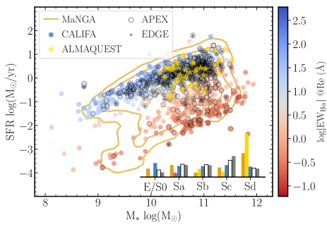
Figure 1: Distribution of the explored galaxies along the SFR-M_∗ diagram. Solid-circles correspond to the extended CALIFA sample, color-coded by the EW(H$\alpha$) at the effective radius of each galaxy. Those galaxies with integrated CO-observations (APEX sub-sample) are represented with an additional black open-circles, while those with spatially resolved CO-observations (EDGE sub-sample) are represented with an additional smaller grey solid-circles. For comparison purposes we include the distribution for the full sample of galaxies explored by ALMaQUEST (yellow solid stars Lin et al., 2020), extracted from the MaNGA survey (Bundy et al., 2015b). The distribution of the full MaNGA sample, DR15 distribution, is represented by successive golden-color density contours (encircling 95%, 40% and 10% of the sample). The inset shows the morphological distribution of galaxies for the different samples (in terms relative), using a similar color-coding: (i) CALIFA in blue, with (ii) APEX in white, including an additional solid black-line, and (ii) EDGE a shaded grey pattern; (iii) ALMaQUEST in yellow and (iv) MaNGA-DR15 in golden colors.

The morphological distributions of all the samples and subsamples included in the diagram are presented in the inset in Figure 1. It is evident that the CALIFA sample covers all the different morphological types, following a more homogeneous distribution than any of the other samples, including the MaNGA DR15. The bias in the morphological distribution of the MaNGA sample with respect to the expected distribution for galaxies in the nearby universe has been discussed before (e.g. Sánchez et al., 2018), and it is beyond the scope of the current article. What it is more relevant is that both the APEX and EDGE sub-samples cover a wide range of galaxy morphologies, with a general trend towards including more late- than early-type galaxies than the original CALIFA sample from which they were drawn. This is understandable since the EDGE sample is clearly biased towards SFGs due to their selection criteria (bright infrared galaxies), and therefore towards later types. However, both samples still include some early-type galaxies and a considerable number of early-spirals (Sb/Sa).

When comparing with the observed distribution for the ALMaQUEST compilation, the first difference to highlight is the lower number of galaxies: 46 objects in the full sample (Lin et al., 2020), with only 14 and 28 of them used in their explorations of the resolved relations (Lin et al., 2019; Ellison et al., 2020a). Furthermore, it is clear that their sample comprises a larger faction of SFGs than either the APEX or EDGE subsamples, with a deficit of retired galaxies (although it covers the Green Valley and comprises several retired regions e.g. Ellison et al., 2020a, b). It also covers a narrower range of stellar masses ($>$10¹⁰M_⊙) and morphologies. The ALMaQUEST sample has a larger fraction late-type galaxies (Sd in most of the cases), with a deficit of early-spirals (in particular, no Sa) and no ellipticals or S0 galaxies. This highlights the importance of revisiting the exploration of the described global and local relations with a different sample to determine the importance (or not) of these selection effects.

It is relevant to highlight that our sample contains a similar number of galaxies as the largest prior explorations of the molecular gas content of galaxies in a redshift range ($z<$0.1) comprise similar number of objects as the one studied here. For instance, the COLD GASS survey, the reference survey in this field (Saintonge et al., 2011), mapped 532 SDSS galaxies using the IRAM-30m telescope. This number of objects is similar to the one comprised by our APEX subsample. It is worth noting that the beam size of their observations is very similar too, so, for galaxies at a similar redshift their molecular gas content is restricted to the same galaxy regions.

In summary, the adopted sample and subsamples are well placed to study the general behaviors of the explored relations due their main properties: (i) they cover a relatively narrow redshift range and a low average redshift ($z\sim$ 0.015), which guarantees a relatively small and quite homogeneous physical resolution ($\sim$800 pc); (ii) the FoV of the IFS explorations ($>~{}$1 arcmin²), that, together with the diameter selection guarantees a large covered optical extent of the galaxies (up to $\sim$2.5 Re) with a good spatial sampling; (iii) the wide range of stellar masses, star-formation stages and galaxy morphologies sampled; and finally, (iv) the spatial coverage and physical resolution of the two datasets of CO observations, that are similar to those of most recent explorations.

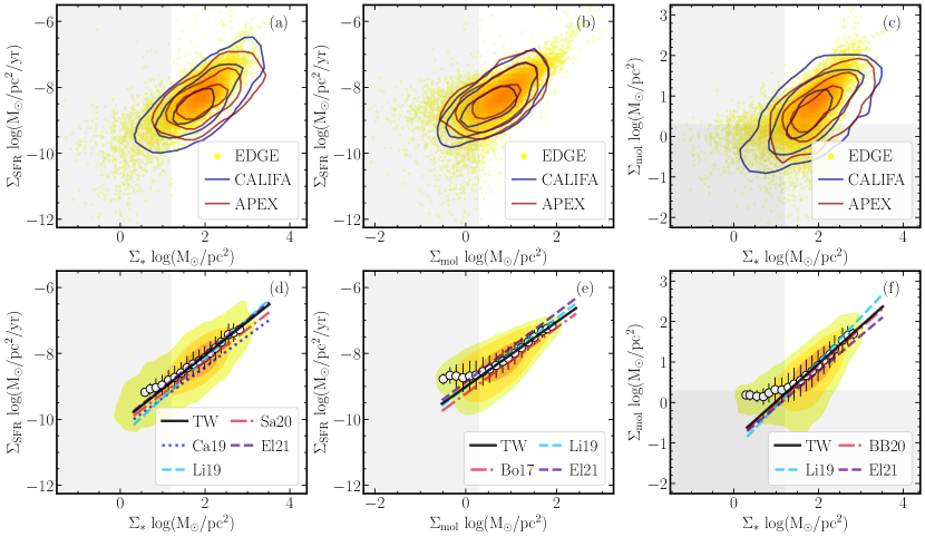
Figure 2: (a) Distribution of $\Sigma_{\rm SFR}$ along $\Sigma_{\rm*}$ for the $\sim$15,000 LoS across the $\sim$100 galaxies observed by the EDGE survey (solid circles, color-coded by the density of points). Blue and red contours show the average $\Sigma_{\rm SFR}$ vs the average $\Sigma_{\rm*}$ for the full CALIFA sample ($\sim$900 galaxies), and the APEX sampled objects ($\sim$400 galaxies). In the case of CALIFA, the values correspond to the average quantities across an effective area (as described in Sec. 3), while in the case of APEX they correspond to the average values within the beam of the antenna. Each consecutive contour encircles 95%, 40% and 10% of each considered sample. Only those LoS (or individual measurements) compatible with ionization dominated by SF, as described in the text, have been included in this plot; (b) and (c) panels show similar distributions for the $\Sigma_{\rm SFR}$ vs. $\Sigma_{\rm mol}$ and $\Sigma_{\rm mol}$ vs. $\Sigma_{\rm*}$ diagrams. Lower panels show the same distributions for the same parameters shown in the corresponding upper panel for the EDGE data, represented as filled contours (with the same encircled number of points as the contours in the upper panels). White solid circles in each lower panel show the mean values in bins of 0.15 dex in the corresponding parameter represented in the X-axis, with error bars indicating the standard deviation around each mean value. The solid black line shows the best fitted linear regression to these solid circles (values within the shadow region, indicating the regime affected by detection issues, were excluded from the fitting). These regressions, labelled as TW (for This Work), correspond to the rSFMS ($d$ panel), rSK ($e$ panel) and rMGMS ($f$ panel), relations. For comparison purposes, we have included some of the most recent derivations of these relations extracted from the literature, including: Bolatto et al. (2017) (Bo17), Lin et al. (2019) (Li19), Cano-Díaz et al. (2019) (Ca19), Barrera-Ballesteros et al. (2020) (BB20), Sánchez et al. (2020) (SS20) and Ellison et al. (2020a) (El21).

3 Analysis and Results

One of the main goals of the current study is to determine how the global intensive relations described for SFGs by the galaxy-wide average $\Sigma_{\rm SFR}$ , $\Sigma_{\rm*}$ and $\Sigma_{\rm mol}$ are connected with the local/resolved relations found between the same quantities at kiloparsec scales. To do so, we follow Sánchez et al. (2020), and derive the described global intensive quantities by dividing each extensive quantity (SFR, M_∗ and M_mol by (i) the effective area of each galaxy (defined as the area within 2r_e, i.e., A_e=4 $\pi$ r${}_{e}^{2}$) for the case of the CALIFA sample, and (ii) the beam area of each CO observation in the case of the APEX subsample (that corresponds in average to $\sim$1 R_e of the galaxies Colombo et al., 2020). For the latter, the choice of area is purely justified by the nature of the observations. In the case of the CALIFA sample, we choose an area representative of the coverage of the IFS data and attached to the properties of each galaxy. However, as already discussed in Cano-Díaz et al. (2019) the use of any area of the order of the size of the FoV of the instrument would provide similar results. The EDGE sub-sample comprises already extensive quantities, as it provides with the spatial resolved $\Sigma_{\rm SFR}$ , $\Sigma_{\rm*}$ and $\Sigma_{\rm mol}$ for the different LoS included in the database (Sec. 2.2. Therefore, no normalization by the area is required). Finally, we apply an inclination correction using the same parameters adopted in the correction of the EDGE dataset (Sec. 2.2). This procedure provides a single set of $\Sigma_{\rm SFR}$ , $\Sigma_{\rm*}$ and $\Sigma_{\rm mol}$ for the subset of SFGs extracted from the CALIFA (532 galaxies) and APEX datasets (251 galaxies). The distribution of these quantities can be then compared directly with kiloparsec scale values provided by the EDGE dataset.

Table 1: Results of the analsys of the rSFMS, rSK and rMGMS scaling relations

Relation	Reference	$\beta$	$\alpha$	rc	$\sigma_{\rm obs}$	$\sigma_{exp}$	# galaxies	# SFA/SFG
rSFMS	EDGE	-10.10$\pm$0.22	1.02$\pm$0.16	0.68	0.266	0.190	126	12667
	CALIFA	-10.27$\pm$0.22	1.01$\pm$0.15	0.85	0.244	0.192	941	533
	APEX	-9.78$\pm$0.30	0.74$\pm$0.21	0.76	0.226	0.211	512	251
	Lin et al. (2019)	-11.68$\pm$0.11	1.19$\pm$0.01		0.25		14	5383∗
	Cano-Díaz et al. (2019)	-10.48$\pm$0.69	0.94$\pm$0.08	0.62	0.27		2737	$\sim$500K
	Sánchez et al. (2020)	-10.35$\pm$0.03	0.98$\pm$0.02	0.96	0.17		1512	$\sim$3M
	Ellison et al. (2020a)	-10.07$\pm$1.44	1.03$\pm$0.17	0.57	0.28-0.39		28	$\sim$15035∗
rSK	EDGE	-9.01$\pm$0.14	0.98$\pm$0.14	0.73	0.249	0.216	126	12667
	CALIFA	-9.01$\pm$0.16	0.95$\pm$0.21	0.77	0.293	0.297	941	533
	APEX	-8.84$\pm$0.24	0.76$\pm$0.27	0.70	0.294	0.228	512	351
	Bolatto et al. (2017)	-9.22	1.00				104	$\sim$5000
	Lin et al. (2019)	-9.33$\pm$0.06	1.05$\pm$0.01		0.19		14	5383∗
	Ellison et al. (2020a)	-8.87$\pm$0.66	1.05$\pm$0.19	0.74	0.22-0.32		28	$\sim$15035∗
rMGMS	EDGE	-0.91$\pm$0.16	0.93$\pm$0.11	0.68	0.218	0.209	126	12667
	CALIFA	-1.12$\pm$0.27	0.93$\pm$0.18	0.74	0.276	0.288	941	533
	APEX	-0.70$\pm$0.37	0.73$\pm$0.24	0.73	0.234	0.212	512	251
	Lin et al. (2019)	-1.19$\pm$0.08	1.10$\pm$0.01		0.20		14	5383∗
	Barrera-Ballesteros et al. (2020)	-0.95	0.93		0.20		93	$\sim$5000
	Ellison et al. (2020a)	-0.99$\pm$0.13	0.88$\pm$0.15	0.72	0.21-0.28		28	$\sim$15035∗

Best fitted intercepts ($\beta$) and slopes ($\alpha$) for the different resolved and global (intensive) relations explored in this article (rSFMS, rSK and rMGMS) and the different explored dataset (EDGE, CALIFA and APEX). Some of the most recent derivations extracted from the literature have been included for comparisons. In addition we include the correlation coefficients ($r_{c}$), the standard deviation around the best fitted relation ($\sigma_{\rm obs}$) and the expected standard deviation due to the error propagation ($\sigma_{\rm exp}$), together with the number of galaxies in each sample and the number of star-forming areas (SFA) or star-forming galaxies (SFG) used in the derivation of the considered relation. $(*)$ We should note that in the case of ALMaQUEST we list the number of spatial elements reported in the quoted articles. However, those are not fully independent measurements, since they adopted the original MaNGA sampling of 0.5$\arcsec$/size spaxels. For a PSF FWHM of $\sim$2.5$\arcsec$, the true number of fully independent measurements (i.e., LoS) would be $\sim$25 lower than the reported values.

Figure 2, top panels, shows the comparison between distributions along the $\Sigma_{\rm SFR}$ -$\Sigma_{\rm*}$ (left), $\Sigma_{\rm SFR}$ -$\Sigma_{\rm mol}$  (middle) and $\Sigma_{\rm mol}$ -$\Sigma_{\rm*}$  (right) diagrams of the global intensive quantities derived for the CALIFA and APEX datasets (as described before) together with the corresponding spatially resolved quantities derived for the EDGE dataset as directly extracted from the database. It is clear that the distributions of the resolved and global parameters cover the same range of values, following the same trends. A simple $\chi^{2}$-test comparing each density distribution indicates that they are statistically indistinguishable when comparing the regions encircled by a 95% of the points (first contours in the upper figures). Significant differences appear only when the comparisons are restricted to the peak of the distributions (region encircling $\sim$20% of the points), in particular when comparing the APEX dataset with the other two. This is expected since the APEX CO observations are restricted to the central $\sim$26$\arcsec$ of the galaxies ($\sim$8 kpc at the average redshift of the sample), and therefore their distribution is slightly shifted towards higher values in the three distributions. However, the effect is insignificant when comparing the full distributions. This indicates that the range of average values covered by the CALIFA and APEX distributions is very similar to the range of spatially resolved values covered with each galaxy. Finally, the distribution for the EDGE dataset enhibits the strongest differences with respect to the other two only in the regimes outside the contour encircling the 95% of the points. Above that density limit this dataset follows in general the same trends as the other two. In summary, this analysis shows that the distributions of the global intensive parameters are the same as those of the resolved ones, as suggested by previous more limited explorations (e.g., Cano-Díaz et al., 2019; Sánchez, 2020; Sánchez et al., 2020). Furthermore, it seems that the caveats regarding the possible biased in the EDGE sub-sample towards SFGs are not relevant for the exploration of these distributions.

Now that we have determined the similarity between the intensive global and resolved distributions, we now characterize the relations among them (i.e., the so-called rSFMS, rSK and rMGMS relations). To do so, we follow a similar procedure as the one performed by previous studies in the characterization of global relations (e.g. Sánchez et al., 2017; Barrera-Ballesteros et al., 2020). First, for each distribution, we derive the median values within a set of consecutive bins of 0.15 dex in the parameter shown in the x-axis of each panel ($\Sigma_{\rm*}$ first and last, and $\Sigma_{\rm mol}$ in the middle one), within the plotted range of values. These bins are restricted to the regime of points encircled by the 95% density contour, in order to exclude outliers. Finally, in the case of the EDGE dataset we restricted our fit to those bins within the 3$\sigma$ detection limits (as reported by Barrera-Ballesteros et al., 2020). These limits are maybe a bit conservative since they refer to the original detection limits of the CO observations, prior to the re-sampling described in Sec. 2, that has certainly increased the signal-to-noise (S/N, per resolution element). The areas below these detection limits are shown as shaded regions in the different panels of Fig. 2. Despite the possible overestimation of the exact value, the individual points in this regime are detected with a low SN, what it is reflected in an increase of the scatter (more clearly appreciated in the $\Sigma_{\rm SFR}$ -$\Sigma_{\rm mol}$ and $\Sigma_{\rm mol}$ -$\Sigma_{\rm*}$ distributions), and a deviation of the average distributions from the general trend.

Fig. 2, bottom panels, illustrates this procedure. The shaded contours show the density distribution of EDGE points in the different panels, and the white solid-points the binned values (with errorbars indicating the standard deviation around the the corresponding value). The solid line (labelled TW, for This Work), describe the best fitted linear relation between each pair of parameters. This relation was performed using a simple linear regression for the white points (weighted by the plotted errorbars, that corresponds to the standard deviation of the distribution), taking into account the restrictions indicated before. In other words, the values were fitted to the expression

$${\mathrm{log}}{\mathrm{P}_{j}}=\beta+\alpha{\mathrm{log}}{\mathrm{P}_{i}}$$ (1)

that corresponds to the power-law $P_{j}=\beta^{\prime}\ {\mathrm{P}_{i}}_{*}^{\alpha}$, where $\beta$=log($\beta^{\prime}$). In order to consider the individual errors, we perform a Monte-Carlo iteration perturbing the original data within their errors, and repeating the full analysis 100 times. The reported relation corresponds to the average of the MC iteration.

Table 1 shows the results of this fitting procedure for the different datasets explored in this study (CALIFA, APEX and EDGE), together with the most recent derivations extracted from the literature. For each of the analyzed relations we present the intercept ($\beta$) and slope ($\alpha$) of the relations, together with the correlation coefficient (r_c) of the original pair of correlated values, and the standard deviation of the y-axis parameter once subtracted the best fitted power-law ($\sigma_{\rm obs}$). For comparison purposes we include the standard deviation that would be expected if the parameters fulfilled perfectly well the derived relations and all the source of dispersion is due to the individual errors ($\sigma_{\rm exp}$). It is important to indicate that literature data have been transformed to our current units (in particular area measured in pc²). As already discussed in Sánchez et al. (2020), the intercept in the reported relations is not a dimensional quantity, and to shift one relation derived for surface densities in kpc² to one in pc², the actual value of the slope ($\alpha$) plays a role. Finally, in the case of Ellison et al. (2020a), that reported two set of values for each relation (based on two different fitting procedures), we list the average of them (corrected to the adopted units too), with the errors corresponding to a 25% of the difference between them.

Focusing on the local/resolved relations, we find good agreement with the results presented by previous explorations. This is particularly true for the slopes of the relations, that in all cases differ less than one or two sigma from those extracted from the literature. The agreement is indeed extremely good with those recently reported by Barrera-Ballesteros et al. (2020) for the rMGMS relation. That is not a surprise since both quantities are derived from the same dataset, although using a different extraction of the LoS. They adopted a less restrictive scheme in terms of the spatial sampling than the one presented here, too. The agreement is also very good with the values reported by Lin et al. (2019) and Ellison et al. (2020a), although there are some appreciable differences. The slopes reported by Lin et al. (2019) are in general larger, although at about one sigma from the ones reported here. Their reported errors for the slopes are much smaller than the ones we find. The differences in the slope are translated to an apparent larger discrepancy in the intercepts. We consider it artificial since it is a consequence of the extrapolation of the relations (with slightly different slopes) to a regime not covered by the observed data (as nicely discussed by Cano-Díaz et al., 2019, recently). This indeed can be appreciated in Fig. 2, lower panels, where we have included the actual relations reported in the literature and listed in Tab. 1, showing a very good agreement with both the ones derived in the current study and the distribution of points for the EDGE dataset.

On the other hand, the average slopes reported by Ellison et al. (2020a) are more similar to the ones reported here. We should note that this study updated the analysis of the ALMaQUEST data by Lin et al. (2019), increasing the number of galaxies by a factor two (and the number of sampled regions by a factor three). In particular, they have a better coverage of the space of parameters, with more green valley galaxies. As discussed in that article the actually fitting procedure matters, with ordinary least squares (OLS) applied to the full sample of regions providing shallower slopes than the one provided by an orthogonal distance regression (ODR) procedure. These later ones are more similar to those reported by Lin et al. (2019). Our current analysis is neither both of them, since it involves a prior binning. We adopted that procedure based in previous experience, and our tests indicate that the recovered values correspond to the real ones within the errors (Sec. 3.3). Finally, we note that the largest difference is found for the relation presented by (Cano-Díaz et al., 2019) for the rSFMS, which in any case is just at one sigma of our observed distribution (i.e., just at the edge of errorbars in the figure).

Having established that our local/resolved relations are similar to the most recent published ones, particularly those using CO observations of similar spatial resolution (e.g. Lin et al., 2019; Ellison et al., 2020a), we continue exploring how those relations compare to the global intensive ones. In the case of the CALIFA dataset, both the intercepts and in particular the slopes agree with the values found for the local relation (EDGE) or reported in the literature (e.g., ALMaQUEST), both listed in Table 1. The main difference, as indicated before, is in the errors reported for both quantities, that in general are larger for the rSK and rMGMS relations. This is expected, since from the CALIFA sample we use an indirect proxy for the molecular gas that most probably adds an extra dispersion in the two relations involving $\Sigma_{\rm mol}$ (Barrera-Ballesteros et al., 2020). The strongest differences are found between the parameters reported for the different relations derived using the APEX dataset when compared with the other two (and the literature values). This may looks contradictory since this dataset comprises molecular masses derived from direct CO observations. However, it is easily understandable when considering that the errors in two estimated coefficients are larger (in some cases considerably larger) than those reported for the derivations based on the CALIFA and EDGE datasets. Indeed, the actual values of the parameters are statistically compatible with those reported for the other datasets (and the literature) within less than one sigma difference. We consider that the combined effect of (i) APEX being the dataset with the lowest number of individual measurements and (ii) its slightly narrower range of covered parameters has produced this effect. Note that although the APEX dataset includes all EDGE galaxies, it comprises only one single set of values per galaxy ($\Sigma_{\rm*}$ , $\Sigma_{\rm SFR}$ , $\Sigma_{\rm mol}$ , aperture matched), not the full range of values covered by the spatially resolved EDGE data. Actually, randomly selecting a similar number of galaxies from the CALIFA dataset, restricted to the same range of parameters covered by APEX, we can reproduce the similar slopes in $\sim$40% of the cases.

As indicated before the errors reported by Lin et al. (2019) in both the intercept and slopes of all the relations are considerably lower than the ones reported here and in most of the studies in the literature. Sánchez et al. (2020) is a counter-example. However, in that particular case only the formal errors with respect to the averaged binned points were reported. This could be well the case for Lin et al. (2019), although they reported an ODR-fitting for the full analyzed dataset. Another possible reason of their low reported errors could be the strong co-variance among their points, since they used individual pixels/spaxels of 0.5$\arcsec$ when their actual PSF FWHM is 2.5$\arcsec$ (i.e., they sampled each resolution element with $\sim$25 non-independent pixels). However, this cannot be the main reason, since in the update analysis of the ALMaQUEST data (with a larger number of measurements) by Ellison et al. (2020a) they reported errors more similar to the ones reported here. Thus, we consider that most probably they have reported just the formal errors.

3.1 Preference among the rSFMS, rSK and rMGMS relations

Lin et al. (2019) reported a clear prevalence among the explored relations, based on the Pearson correlation coefficient and the standard deviations of the residuals (i.e., once subtracted the best fitted model). Based on their analysis the rSK is the primary relation between the explored parameters, with a correlation coefficient significantly larger (r${}_{c}=$0.81), and a standard deviation slightly lower ($\sigma=$0.19 dex), than that of the other two (r_c=0.76 and 0.64, and $\sigma=$0.20 and 0.25 dex, for the rMGMS and rSFMS respectively). Their conclusion is that the combination of the rSK and rMGMS relations leads to the rSFMS as a by-product of the other two correlations. Similar results were found in the updated analysis by Ellison et al. (2020a), in the sense that the rMGMS and rSK present a tighter correlation (lower standard deviations) than the rSFMS. So far, we cannot confirm their results and conclusions. Neither for the resolved nor for the intensive global relations explored in here we find a clear prevalence among them. For the EDGE dataset the correlation coefficients are essentially equal among the different explored relations, with an r${}_{c}\sim$0.68-0.73, as seen in Tab. 1. Although the strongest correlation is found for the rSK (r${}_{c}=$0.73), there is neither such a big difference as the one reported by Lin et al. (2019), nor a clear ordering (indeed, the r_c found for the rSFMS is the same as the one found for the rMGMS). Furthermore, the minimum standard deviation of the residual is found for the rMGMS ($\sigma_{\rm obs}=$0.218 dex), and not for the rSK. Indeed, this later one exhibits a standard deviation of the residual just slightly lower than that of the rSFMS ($\sigma_{\rm obs}=$0.249 and 0.266 dex, respectively). For a proper comparison among the different relations is needed to consider the expected standard deviation due to the propagation of the errors in the observed quantities and the estimated slopes ($\sigma_{\rm exp}$ in Tab. 1). When doing so we find that the rMGMS is indeed the relation with the smallest residuals, with a dispersion essentially dominated by the errors, with the rSFMS being the one with the largest dispersion, on the other hand (with an intrinsic dispersion $\sim$0.066 dex). Note that we have included the third decimal to reveal any possible difference, although we find it difficult to justify the significance of any decimal beyond the second one.

Similar results are found for the aperture-limited and global intensive scaling relations. In the case of the APEX dataset, the rSK relation is the one with the weakest correlation (r_c=0.73), having the largest standard deviations of the residuals ($\sigma_{\rm obs}=$0.294 dex vs. $\sigma_{\rm exp}=$0.228 dex), with the rSFMS the one that shows the strongest one (r_c=0.76), with the lowest standard deviation ($\sigma_{\rm obs}=$0.226 dex vs $\sigma_{\rm exp}=$0.211 dex).

Figure 3: Distribution of $\Sigma_{\rm SFR}$ , $\Sigma_{\rm mol}$ and $\Sigma_{\rm*}$ in three dimensional space for CALIFA (averaged across each galaxy, left panel), APEX (averages across the antenna beam, middle panel), and EDGE (individual kpc-scale LoS, right panel). Each galaxy (CALIFA/APEX) or region within a galaxy (EDGE) is represented as a single solid circle, both in the 3D space and projected in each axis. Each circle is color-coded according to the local 3d density of points. Contours in each axis represent the regions encircling a 95%, 40% and 10% of the points. Semi-transparent planes, and their corresponding projections in each axis, describe the location of the best fitted planes to the observed distribution of points assuming: (i) that $\Sigma_{\rm SFR}$  depends on both $\Sigma_{\rm*}$ and $\Sigma_{\rm mol}$ (i.e., that those parameters are independent), represented by a grey plane (in 3d) and three black-dotted lines (in each axis), i.e., the “Plane”-model approach, as described in the text; and (ii) that there is no a priori knowledge of which is the dependent or independent parameter, represented by a blue plane (in 3d) and three blue-dashed lines (in each axis). Thus, the “PCA”-model approach, as described in the text. The estimated parameters describing each plane are included in the inset label. Solid dark-red lines in each axis correspond to the best fitted linear regressions to each pair of data derived using the procedure outlined in Fig. 2, i.e., the rSFMS, rSK and rMGMS relations. In addition, the average of the rSFMS and rSK relations, and their projection in the $\Sigma_{\rm mol}$ -$\Sigma_{\rm*}$ plane, is shown as a dashed-dotted 3D line too. This is the first functional form adopted to describe a average ”Line”-model, as indicated in the text. It is evident from the figure that none of the planes described before (grey or blue), nor their projections in the axis, describes the distribution of points as well as the 3D dark-red solid line, as discussed in the text. Finally, the solid black-line, in each panel, corresponds to the best-fitted line in the three dimensional space derived using a simple linear regression. A version of this figure for different projection angles is included in the following link: http://ifs.astroscu.unam.mx/CALIFA/EDGE/Scaling_Relations/

Finally, for the CALIFA dataset the strongest correlation is the one found for the rSFMS (r_c=0.85), followed by the one for the rSK (r_c=0.77), that it is just slightly larger than that of the rMGMS (r_c=0.74). The rSFMS is the relation with the lowest observed standard deviation, too ($\sigma_{\rm obs}=$0.244 dex), with the rSK exhibiting the largest one ($\sigma_{\rm obs}=$0.294 dex). However, in this case, when comparing with the expected standard deviations due to the errors we observe that indeed both the rSK and rMGMS are completely dominated by them ($\sigma_{\rm obs}=$0.297 dex and $\sigma_{\rm exp}=$0.288 dex, respectively).

The relative weakness of the relations involving $\Sigma_{\rm mol}$  for CALIFA (compared with the rSFMS one) could be attributed to some extent to the fact that the gas mass is derived using an indirect proxy (with the largest errors with respect to the rest of the involved analyzed quantities). However, this does not change (or affect) the fact that the correlation coefficient derived for the rSFMS in this dataset is the strongest among all the explored relations. Indeed, the strength of the resolved rSFMS reported by Lin et al. (2019) and Ellison et al. (2020a) are among the weakest found in the literature (see Tab. 1). For instance, Cano-Díaz et al. (2016a) and Cano-Díaz et al. (2019), based on the exploration of the star-forming regions in the CALIFA and MaNGA-DR15 dataset respectively, found a correlation coefficient of $\sim$0.85 in both cases (equal to the one presented here). We cannot be certain of the nature of the difference, but we speculate that the limitations of their explored sample (14 and 28 galaxies respectively, limited range of stellar masses, aperture limitation of the MaNGA IFU data), could affect the strength of the resolved rSFMS relation somehow. But we cannot be conclusive in this regards.

In conclusion, we do not find a significant prevalence among the scaling relations either at local or galaxy-wide scales, in contrast with previous studies. The results for the different subsamples are contradictory, and the comparison between the correlation coefficients and both the observed and intrinsic dispersion of the relations do not provide with a consistent picture. In some cases the strongest correlation does not correspond with the lowest intrinsic dispersion (e.g., CALIFA/rSFMS, EDGE/rSK relations), and in general the strongest correlation is not always the same of the different datasets (rSFMS for CALIFA and APEX, rSK for EDGE). Finally, in most of the cases there is no significant difference between the observed standard deviations of the residuals and the expected one due to error. The largest differences are found for the rSFMS, in the case of EDGE and CALIFA ($\sim$0.05-0.06 dex), and for the rSK, in the case of APEX ($\sim$0.07 dex). Even in these cases is difficult to justify their significance.

3.2 Which parametrization best describes the $\Sigma_{\rm SFR}$ ?

In the previous sections we established that the three explored parameters ($\Sigma_{\rm*}$ , $\Sigma_{\rm mol}$ and $\Sigma_{\rm SFR}$ ) correlate with one each other in a similar way at both kpc-scales and averaged galaxy-wide. Following Lin et al. (2019) and Ellison et al. (2020a), we tried to establish a prevalence among the reported relations. However, we did not find a clear one. The explanation offered by the prevalence proposed by Lin et al. (2019) and Ellison et al. (2020a) is appealing. To consider the $\Sigma_{\rm mol}$  as the main driver of the star-formation process fits with our understanding of the physical process at low physical scales, as first proposed in the seminal studies by Schmidt (1959) and Kennicutt (1998b), and explored recently using spatially resolved CO observations (e.g. Leroy et al., 2013). However, this view does not fit with the picture emerging from the exploration of galaxy wide relations, like the global (extensive) SFMS, in which the role of the depth of the stellar potential seems to govern the SF (e.g. Saintonge et al., 2011). However, the discovery of the resolved rSFMS relation (Sánchez et al., 2013; Wuyts et al., 2013) required redefining this interpretation for a local one, in which the SF depends on the local depth of the gravitational potential traced by $\Sigma_{\rm*}$ (Sánchez, 2020).

The quest for a more global star-formation law, that includes both parameter ($\Sigma_{\rm mol}$ and $\Sigma_{\rm*}$ ), or even additional ones that trace the dynamics of galaxies and regions within galaxies, have led to different functional forms. The seminal work of Elmegreen (1993), Wong & Blitz (2002), and Blitz & Rosolowsky (2004, 2006) established the importance of the interstellar medium pressure, which depends on the gravitational field and hence the stellar mass, on determining the density of the star forming gas and the atomic to molecular transition. Shi et al. (2011) and Shi et al. (2018) proposed a dependence between $\Sigma_{\rm SFR}$ and a combination of the other two parameters with the form $\Sigma_{\rm mol}$ $\times$$\Sigma_{\rm*}$ ^-β (with $\beta$=0.5), following a power-law as the one followed by the relations explored along this study. This parametrization was motivated by the proposed effect of the mid-plane pressure in self-regulating the star-formation process (e.g. Ostriker et al., 2010). This parameterization was explored by Lin et al. (2019), finding that a value of $\beta$=0.3 slightly improves the dispersion with respect to the one reported for the original rSK one, for a slope of $\alpha$=1.38, in the overall power-law. Thus, they proposed that the generalized star-forming law should exhibit the form $\Sigma_{\rm SFR}\propto\Sigma_{\rm mol}^{1.38}\Sigma_{*}^{-0.39}$. However, we should note that they did attempt to attribute this parametrization to the need for a secondary dependence, in an explicit way, and indeed they concluded that the original rSK form is sufficient to describe the observed distributions.

In an almost simultaneous study, Dey et al. (2019) explored a more generalised relation to describe $\Sigma_{\rm*}$ using not only $\Sigma_{\rm mol}$ and $\Sigma_{\rm*}$ , but including a plethora of additional parameters, such as both resolved and global properties of galaxies, and dynamical, stellar population and ionized gas properties. Their exploration was based on a subset of 38 galaxies extracted from the current EDGE sample, although using a preliminary extraction of both the CO and optically based dataproducts. They used a Least Absolute Shrinkage and Selection Operator to identify which of the explored properties significantly influence the $\Sigma_{\rm SFR}$ . Then, selecting those that strongly predict the star-formation, they proposed a relation based on eight parameters, with the functional form $\Sigma_{\rm SFR}\propto\Sigma_{\rm mol}^{0.4}\Sigma_{*}^{0.7}R^{0.6}\tau_{*}^{-0.6}\sigma_{*}^{0.2}Z_{\rm gas}^{-2.7}$, where $R$ is the galactocentric distance normalized by the effective radius of the galaxy, $\tau_{*}$ is the mass-weighted stellar age, $\sigma_{*}$ is the stellar velocity dispersion and $Z_{\rm gas}$ is the solar-normalized gas oxygen abundance.

The first thing to notice is that both relations predict a totally different dependence of $\Sigma_{\rm SFR}$ on the $\Sigma_{\rm*}$ . While the physically motivated functional form explored by Lin et al. (2019) proposes a relation in which $\Sigma_{\rm*}$ presents a negative slope, on the contrary to $\Sigma_{\rm mol}$ , the empirical one proposed by Dey et al. (2019) uses a positive slope for both parameters. In other words, the first relation follows a trend consistent with the rSK, but not with the rSFMS, while the second one follows a trend qualitatively consistent with both relations.

Table 2: Results of the exploration of the distribution in the 3D space

Relation	Dataset	$a$	$b$	$c$	$d$	rc	$\sigma$
Plane	EDGE	0.439$\pm$0.005	0.566$\pm$0.005	-1	9.504$\pm$0.008	0.72	0.257
	CALIFA	0.657$\pm$0.015	0.383$\pm$0.024	-1	9.887$\pm$0.049	0.85	0.246
	APEX	0.466$\pm$0.021	0.323$\pm$0.019	-1	9.497$\pm$0.039	0.74	0.234
PCA	EDGE	0.751$\pm$0.004	0.002$\pm$0.008	-0.662$\pm$0.004	6.810$\pm$0.031	0.64	0.307
	CALIFA	0.734$\pm$0.021	0.076$\pm$0.043	-0.679$\pm$0.026	7.133$\pm$0.160	0.83	0.278
	APEX	0.697$\pm$0.112	-0.195$\pm$0.390	-0.569$\pm$0.151	6.024$\pm$1.343	0.59	0.356
Line	EDGE	0.510$\pm$0.008	0.490$\pm$0.070	-1	9.555$\pm$0.180	0.77	0.232
	CALIFA	0.505$\pm$0.075	0.475$\pm$0.105	-1	9.640$\pm$0.190	0.88	0.231
	APEX	0.370$\pm$0.105	0.380$\pm$0.135	-1	9.310$\pm$0.270	0.79	0.217

Best fitted parameters ($a$,$b$,$c$ and $d$), under the three different assumptions included in this study (Plane, PCA or Line), and the different explored dataset (EDGE, CALIFA and APEX), for the functional form $\Sigma_{*}^{a}\Sigma_{\rm mol}^{b}\Sigma_{\rm SFR}^{c}=10^{d}$, together with the correlation coefficient (r_c) and the standard deviation of $\Sigma_{\rm SFR}$ once the best fitted model is subtracted ($\sigma$). For the ”Line” we list parameters of the average between the rSK and rSFMS, that would require also a rMGMS to define a line in the 3D space.

If all the parameters adopted to build the independent parameter in both relations would be totally independent, i.e., not presenting any relation among themselves, the $\Sigma_{\rm SFR}$ would follow a plane in the hyper-space of parameters. In the case of the functional form proposed by Lin et al. (2019) a plane in the $\Sigma_{\rm*}$ ,$\Sigma_{\rm mol}$ and $\Sigma_{\rm SFR}$ three-dimension space (although we should clarify that they never claim that the distribution follows a plane, and the dataset shown in the 3D space in their Fig. 1 could be well described as a cylinder). On the other hand, if the parameters entering in the equation are fully dependent to each other, the $\Sigma_{\rm SFR}$ should follow a line in the hyperspace (but not a plane). Indeed, Dey et al. (2019) presented the existing relations between the different additional parameters including in their functional form. This result, and the existence of the rSFMS, rSK and rMGMS relations themselves, explored in the previous sections, supports more the second interpretation than the first one. In other words, the three parameters $\Sigma_{\rm*}$ ,$\Sigma_{\rm mol}$ and $\Sigma_{\rm SFR}$ depend to each other. However, in this case, a different sign in the slope for the $\Sigma_{\rm mol}$ and $\Sigma_{\rm*}$ in the proposed relations is not clearly justified (since it naturally described a plane, not a line).

We explore here three different possibilities to describe the relation among the three considered parameters in order to understand which one describes better the observed distribution. To do so we determine which of them has the strongest correlation and the minimum standard deviation of the residuals for the $\Sigma_{\rm SFR}$ . We define those three possibilities as:

• Plane: We consider that $\Sigma_{\rm SFR}$ is the truly dependent parameter, with $\Sigma_{\rm mol}$ and $\Sigma_{\rm*}$ being the independent ones. This way the distribution is described by a plane with the functional form:

  $$\begin{matrix}\Sigma_{\rm SFR}\propto\Sigma_{*}^{a}\Sigma_{\rm mol}^{b}\end{matrix}$$ (2)

  We use the same least-square minimization adopted for the analysis of the individual relations described in the previous sections to fit the data, with the exception that we use the full set of data, not a binning scheme as the one adopted before. We should note that based on the results in the previous section, and recent results in the literature (Lin et al., 2019; Ellison et al., 2020d; Sánchez et al., 2020), it is clear that choosing $\Sigma_{\rm SFR}$ as the dependent parameter is somehow arbitrary. Furthermore, it is also clear that $\Sigma_{\rm mol}$ and $\Sigma_{\rm*}$ are not fully independent one each other. We adopted the current functional form following the literature in this topic, and in particular the search for a generalized SF-law (Shi et al., 2011, 2018; Barrera-Ballesteros et al., 2021a)

• PCA: We consider that we do not know a priori which is the independent parameter of the three. However, we assume that the distribution is well described by a plane in the three dimensional space, following the functional form:

  $$\begin{matrix}\Sigma_{*}^{a}\Sigma_{\rm mol}^{b}\Sigma_{\rm SFR}^{c}=10^{d}\end{matrix}$$ (3)

  Then, we perform a Principal Component Analysis (PCA hereafter) to determine the parameters that describe better this plane, without assuming which is the dependent parameter (we adopted the PCA algorithm included in the scikit-learn package implemented in python). Note that under this nomenclature the previously fitted functional form would be the same, fixing $c=$-1.

• Line: Finally, we consider that the parameters follow a line in the three dimensional space (or 3D-line), instead of a plane. For a first approximation we derive this line as the intersection of the rMGMS ($\Sigma_{*}^{\alpha_{\rm rMGMS}}\Sigma_{\rm mol}^{-1}=10^{-\beta_{\rm rMGMS}}$) with the plane resulting from the average of the sSK and rSFMS relations discussed before (Fig. 2, Tab. 1):

  $$\begin{matrix}\Sigma_{*}^{0.5\alpha_{\rm rSFMS}}\Sigma_{\rm mol}^{0.5\alpha_{\rm rSK}}\Sigma_{\rm SFR}^{-1}=10^{-(\beta_{\rm rSK}+\beta_{\rm rSFMS})}\end{matrix}$$ (4)

  This approach for defining a 3D-line allows us to compare the coefficients of Eq. 4 with those provided by the two other methods (Eq. 2 and 3). However, it does not provide us with the real functional form for the best three dimensional line describing the data, being just a first approximation. For completeness, we derive this line too by a simple linear regression to the data. Note that neither of these lines are the intersection of the previous fitted planes. If that were the case we would not expect the line to improve the representation of the data.

Table 3: Best fitted linear regression in the 3D space to a single line

Dataset	$a_{*}$	$b_{*}$	$a_{\rm SFR}$	$b_{\rm SFR}$	$a_{\rm mol}$	$b_{\rm mol}$	$\sigma$
EDGE	1.740 $\pm$ 0.005	1.222 $\pm$ 0.011	0.683 $\pm$ 0.005	0.762 $\pm$ 0.013	-8.322 $\pm$ 0.005	1.016 $\pm$ 0.014	0.185
CALIFA	1.862 $\pm$ 0.030	1.156 $\pm$ 0.067	0.615 $\pm$ 0.025	0.790 $\pm$ 0.045	-8.445 $\pm$ 0.040	1.053 $\pm$ 0.045	0.248
APEX	2.033 $\pm$ 0.045	1.293 $\pm$ 0.073	0.691 $\pm$ 0.050	0.834 $\pm$ 0.081	-8.332 $\pm$ 0.030	0.873 $\pm$ 0.087	0.241

Best fitted parameters ($a_{par}$ and $b_{par}$), of the parametrization of the data in the three-dimensional space by a line, following the functional form described in Eq. 6. The standard deviation of $\Delta$$\Sigma_{\rm SFR}$ of the different datasets with respect to the best fitted line is also included ($\sigma$).

This analysis and its results are illustrated in Figure 3, comprising the three dimensional distribution of the considered parameters ($\Sigma_{\rm SFR}$ , $\Sigma_{\rm*}$ and $\Sigma_{\rm mol}$ ) for the three different samples adopted in this article, together with the best fitted models following the four approaches. These values, together with the correlation coefficient and the dispersion once the best model is subtracted, for the first three adopted functional forms, are listed in Table 2. As expected the first two approaches (Plane and PCA) do not provide linear distributions along the 3D space. But instead both describe a plane, whose projection in the three axes can not reproduce the three relations explored in the previous sections (rSFMS, rSK and rMGMS).

In the case of $\Sigma_{\rm SFR}$ being a fully dependent parameter of the other two (Plane case), the best fitted model produces qualitatively well the results by Dey et al. (2019), with the two powers of the $\Sigma_{\rm mol}$ and $\Sigma_{\rm*}$ parameters having the same sign (both positive). In the case of the CALIFA and EDGE datasets the actual values of the slopes match within 0.1 dex with respect to the reported ones. It is interesting to note the projection of the “Plane” relation passes through the distributions in the $\Sigma_{\rm SFR}$ -$\Sigma_{\rm*}$ and $\Sigma_{\rm SFR}$ -$\Sigma_{\rm mol}$ planes, following the expected trends, but with considerably shallower slopes. On the other hand, it cannot describe the distribution in the $\Sigma_{\rm mol}$ -$\Sigma_{\rm*}$ plane, since it assumes that both parameters are independent. Curiously, the introduction of this functional form to describe the $\Sigma_{\rm SFR}$ does not significantly improve the characterization of the data. Both the correlation coefficients and the standard deviations of the residuals are the same or worse than those reported for the rSFMS as listed in Tab. 1. In the case of the rSK, the correlation coefficient of the “Plane” model is improved only for the APEX and CALIFA datasets, with a decrease of the standard deviation only significant for the later one. For the APEX dataset, there is no improvement for the rSK in any of the two parameters.

The PCA analysis tries to reproduce the plane in the space of parameters using the linear combination of the parameters that retains most of the variance of the distribution, thereby minimizing the residuals with respect to the derived model. This analysis does not require assuming which is the dependent parameter, as indicated before. In this regard it is interesting to note that our current analysis attributes the lowest variance to $\Sigma_{\rm mol}$ , and it seems that most of it is attributed to the combination of $\Sigma_{\rm SFR}$ and $\Sigma_{\rm*}$ , i.e., the two parameters involved in the rSFMS. Based on our results, this procedure yields a plane in the 3D space, the projections of which reproduce this relation better than any of the other two. Indeed, for the $\Sigma_{\rm mol}$ -$\Sigma_{\rm*}$ plane, the projection seems to be orthogonal to the best fitted rMGMS. The power law index (slope) of the relation attributed to $\Sigma_{\rm mol}$ is small, almost consistent with zero. As in the case of the Plane approach, the best fitted models do not provide an improvement of the characterization in terms of the standard deviations of the residuals (Tab. 1 vs. Tab. 2). Actually, the residuals are larger than the ones produced by the three originally explored relations (rSFMS, rSK and rMGMS), for any of the explored datasets. On the contrary, the correlation coefficients are similar, just slightly worse (CALIFA and APEX), or slightly better (EDGE) than the ones provided by the Plane-model. It is worth noting that despite their physical motivation, neither the Plane nor the PCA procedures reproduce the coefficients of the plane proposed by Shi et al. (2011) or Lin et al. (2019).

Figure 4: Distribution of the residuals along the perpendicular plane to the best fitted 3D-line representing the EDGE dataset (solid-line in Fig. 3, Tab. 3). Both axes ($u$,$v$) do not fully corresponds to any of the explored parameters, due to the projection, although $u$ is almost parallel to $\Sigma_{\rm mol}$ and $v$ to $\Sigma_{\rm SFR}$ (due to a pure mathematical artifact). Individual LoS are represented by solid circles, following the same scheme adopted in Fig. 2. The standard deviation of the distribution in the y-axis is included in the corresponding inset. Contours in each panel corresponds to the area encircling 95%, 80% and 40% of the datapoints (black solid lines).

The 3D line resulting from the average of the rSFMS and rSK relations (Eq. 4), together with the rMGMS reported in the previous section (values in Tab. 1), shows the best characterization of the data. The standard deviation of the residuals is clearly the lowest of the three explored approaches, for the three datasets. It presents a lower standard deviation that the original rSFMS and rSK relations too. It also exhibits the strongest correlation coefficients, improving upon the previous parametrizations in all datasets. By construction, it reproduces the two relations from which it is created. We note that if, instead of combining the rSFMS and rSK to reproduce the distribution in the 3D space we adopt any other combination of relations, we would derive very similar results. This is a consequence of the fact that the three parameters ($\Sigma_{\rm*}$ , $\Sigma_{\rm SFR}$ and $\Sigma_{\rm mol}$ ) follow a line in the 3D space. For instance, it is easy to demonstrate that if the data fulfill simultaneously the rSK and rSFMS relations, then $\Sigma_{\rm mol}$ and $\Sigma_{\rm*}$ cannot be independent parameters. By just solving the equation:

$$\begin{matrix}\beta_{\rm SFMS}+\alpha_{\rm SFMS}{\rm log}(\Sigma_{\rm*})={\rm log}(\Sigma_{\rm SFR})=\beta_{\rm SK}+\alpha_{\rm SK}{\rm log}(\Sigma_{\rm mol})\end{matrix}$$ (5)

we would derive a rMGMS relation, the coefficients of which are fully consistent with the ones listed in Tab. 1. This is apparent in Fig. 3, where we show that this inferred rMGMS relation (represented as dotted-dashed line in Fig. 3) is in excellent agreement with the best fitted one (represented as a solid-line in the same figure). It is important to note that we were unable to attain such a result when using the Plane or PCA parametrizations of the relations.

Figure 5: Distribution of the residuals of the three relations explored along this study one versus another: (i) $\Delta$rSFMS vs $\Delta$rSK (left panel); (ii) $\Delta$rSFMS vs. $\Delta$rMGMS (central panel); and (iii) $\Delta$rSK vs. $\Delta$rMGMS (right panel). Individual LoS (solid circles, color coded by the density of points), mean values in bins of 0.15 dex of the parameter in the X-axis (white circles), and the best fitted linear regression (solid line) are represented in each panel following the same scheme adopted in Fig. 2. The parameters of the best fitted linear regression, following Eq. 1, together with the standard deviation of the residuals and the correlation coefficients between the datasets shown in each panel are included in the corresponding inset. Contours in each panel corresponds to the area encircling 95%, 80% and 40% of the datapoints (black solid lines).

Finally, we find the best parametrization of this 3D line using a simple linear regression of the dataset, corresponding to the black-solid line shown in each panel of Fig. 3. This line has the functional form:

$$\begin{pmatrix}{\rm log}\Sigma_{\rm*}\\ {\rm log}\Sigma_{\rm SFR}\\ {\rm log}\Sigma_{\rm mol}\\ \end{pmatrix}=\begin{pmatrix}a_{*}\\ a_{\rm SFR}\\ a_{\rm mol}\\ \end{pmatrix}+\begin{pmatrix}b_{*}\\ b_{\rm SFR}\\ b_{\rm mol}\\ \end{pmatrix}\times t$$ (6)

where $t$ is the independent parameter tracing the linear distribution, and parameters $a$ and $b$ are the coefficients describing the 3D line for each explored physical property. This parametrization can be written in a functional form more similar to Eq. 5, by solving $\Sigma_{\rm SFR}$ :

$$\begin{split}\frac{{\rm log}(\Sigma_{\rm*})-a_{\rm*}}{b_{\rm*}}=\frac{{\rm log}(\Sigma_{\rm SFR})-a_{\rm SFR}}{b_{\rm SFR}}=\frac{{\rm log}(\Sigma_{\rm mol})-a_{\rm mol}}{b_{\rm mol}}\\ b_{\rm SFR}\frac{{\rm log}(\Sigma_{\rm*})-a_{\rm*}}{b_{\rm*}}+a_{\rm SFR}={\rm log}(\Sigma_{\rm SFR})=b_{\rm SFR}\frac{{\rm log}(\Sigma_{\rm mol})-a_{\rm mol}}{b_{\rm mol}}+a_{\rm SFR}\end{split}$$ (7)

This way it is possible to compare the coefficients of the parametrization to those listed in Tab. 1 and 2. Table 3 lists the estimated values for the coefficients and the standard deviation of the residual with respect to the best fitted line. For the three datasets we derive very similar coefficients, in particular for the slope ($b$) of the linear relation. The steeper slope corresponds to the one for the $\Sigma_{\rm*}$ relation (being slightly higher than one), and the shallower one for the $\Sigma_{\rm SFR}$ (being slightly lower than one). The residuals for $\Sigma_{\rm SFR}$ around the best fitted 3D line are very similar among the different datasets, being of the order of those reported for the average line (Table 2).

As a final check, we present in Figure 4 the distribution of residuals across the plane perpendicular to this best fitted 3D-line for the EDGE dataset (the axis are labeled $u$ and $v$, representing the directions perpendicular to the line in Eq. 6). If the distribution along the 3D-space is sufficiently well represented by a 3D-line, then these residuals should not present any elongation. In contrast, if a plane describes better the observed distribution, those residuals should present a detectable elongation along the direction defined by the plane itself. As apparent in the figure the residuals present no elongation along a preferred direction, with a negligible correlation coefficient. We note that in principle the axes represented in this figure do not necessarily correspond to any of the three physical quantities explored here. Nonetheless, it turns out that $v$ is almost parallel to $\Sigma_{\rm SFR}$ with a scaling factor $\sim 0.762$ (the slope of the 3D-line for this parameter, Tab. 3). We also note that the standard deviation in Fig. 4 fully matches the one enlisted in Tab. 3 for $\Sigma_{\rm SFR}$ , once the scaling factor is taken into account. Similar results are found for the APEX and CALIFA datasets.

In summary, this final test reinforces our results showing that the distribution in the 3D space is best represented by a line, from which the previous relations are pure projections. Therefore, there is no preference among the rSFMS, rSK and rMGMS relations in their description of the observed distributions. We will discuss the implications later in Sec. 4.

3.3 Exploring possible secondary relations

In the two previous sections we have characterized the paired relations between the $\Sigma_{\rm SFR}$ , $\Sigma_{\rm*}$ and $\Sigma_{\rm mol}$ (i.e., the rSFMS, rMGMS and rSK relations), showing that they follow a log-log relation in the space defined by them that is well characterized by a 3D-line. This analysis shows that the distribution is not well represented by a plane or a surface. This, in essence, limits the possibility of a third parameter that significantly contributes to the dispersion in the analyzed relations, at least a parameter among the ones explored here or well-correlated with them. In other words, if the relation followed by the three parameters is a line and not a plane, the residual in any of the explored relations (e.g., the rSFMS) should not depend significantly on any parameter that includes the third explored parameter ( this is, $\Sigma_{\rm mol}$ , in the case case that the explored relation is rSFMS). However, previous studies have indicated that some of these relations show explicit dependencies with a third parameter. For instance, González Delgado et al. (2016) and Cano-Díaz et al. (2019) show that the the rSFMS segregates by morphology, with SF regions in later-type galaxies having slightly larger $\Sigma_{\rm SFR}$ for a fixed $\Sigma_{\rm*}$ than earlier types. Since morphology is directly connected with star-formation stage, $f_{gas}$ and SFE (e.g. Saintonge et al., 2016; Calette et al., 2018; Sánchez et al., 2018), then any morphological difference may be interpreted as a difference induced by a third additional parameter. Indeed, some authors (e.g. Ellison et al., 2020d) have reported that the observed scatter in the rSFMS depends both on the star-formation efficiency (SFE) and the molecular gas fraction ($f_{mol}$), with a prevalence for the first parameter. Others explorations of the integrated SFMS ( for only SFGs) suggest that the scatter depends more on the gas fraction rather than on the SFE (e.g. Saintonge et al., 2016; Sánchez et al., 2018; Colombo et al., 2020). In some cases, the differences in the relation found galaxy by galaxy have led to some authors to claim that indeed there is no general rSFMS relation (e.g. Vulcani et al., 2019), which is totally contrary to most previous results (as reviewed by Sánchez, 2020). Finally, the search for a third parameter to reduce the scatter of the observed relations has led to modifications of the rSK law, which includes $\Sigma_{\rm*}$ (known as the extended Schmidt-law, e.g. Shi et al., 2011) and other resolved and integrated parameters (e.g. Dey et al., 2019), as indicated in the previous section.

The main hypotheses behind these different explorations are that (i) indeed the scatter in the relations depends on a third parameter, (ii) the residual of the considered relation correlates with either a parameter (or property), a combination of parameters, or the residuals of another relation, and (iii) that this new correlation is physically driven, significant, decreasing the scatter around the original relation and altering significantly its shape. For instance, Table 2 of Cano-Díaz et al. (2019) shows that the shape of the rSFMS (its intercept and slope) for SF regions is different for different morphological types. In the same way, Ellison et al. (2020d), shown in their Fig. 4, that the residual of the rSFMS strongly correlates with that of the rSK (a parameter that tightly correlates with the SFE if the slope of rSK is near to one). However, none of them shows a really clear and significant decrease of the original scatter when these possible secondary relations are introduced. On the contrary, Dey et al. (2019) and Lin et al. (2019) show a decrease of the scatter of the original relation (rSK and rSFMS, respectively), when additional parameters are included in the parametrization of the relations.

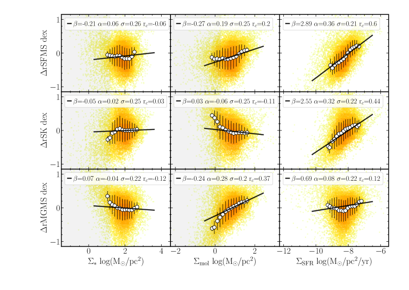
Figure 6: Residuals of the rSFMS (top panels), rSK (middle panels), and rMGMS (bottom panels) along the $\Sigma_{\rm*}$ (left panels), $\Sigma_{\rm mol}$ (middle panels) and $\Sigma_{\rm SFR}$ (right panels) for the EDGE dataset. Individual LoS (solid circles, color coded by the density of points), mean values in bins of 0.15 dex of the parameter in the X-axis (white circles), and the best fitted linear regression (solid line) are represented in each panel following the same scheme adopted in Fig. 2. The parameters of the best fitted linear regression, following Eq. 1, together with the standard deviation of the residuals and the correlation coefficients between the datasets shown in each panel are included in the corresponding inset.

Based on the previous section results, we would expect little or no dependence either between the residuals of the explored relations or between those residuals and a third parameter not considered in the relations. To explore this possibility in the most ample and agnostic way we first explore the residuals of the three relations one versus each other (following Ellison et al., 2020d) that is, the relations between $\Delta$rSFMS, $\Delta$rSK and $\Delta$rMGMS where residual is defined as the removal of the “best fit” relation from the measurement of the dependent parameter (for example, removing the rSFMS from the measured value of $\Sigma_{\rm SFR}$ for a given $\Sigma_{\rm*}$ ). Figure 5 shows the results of this exploration. Contrary to what would be naively expected from the results presented in the previous sections there is a clear correlation between the three residuals. The strongest one is the one between $\Delta$rSFMS and $\Delta$rSK, that it is just slightly less strong and shows the same slope as the one presented by Ellison et al. (2020d), in their Fig. 4. It is followed by the relation between $\Delta$rSFMS and $\Delta$rMGMS, and finally by the one between $\Delta$rSK and $\Delta$rMGMS. The correlation coefficients in the three cases are larger than 0.4. In the case of the rSFMS there is a small but appreciable decrease of the scatter with respect to the original relation for both the tentative secondary relation with the $\Delta$rSK and $\Delta$rMGMS. If these secondary relations were physically motivated, our conclusions would be similar to the ones presented by Ellison et al. (2020d), suggesting that the scatter of the rSFMS is driven mostly by the SFE ($\sim$$\Delta$rSK, in particular when $\alpha=$1). Furthermore, we could conclude that the scatter in the rSK is partially due to gas fraction (f_gas$\approx$$\Delta$rMGMS).

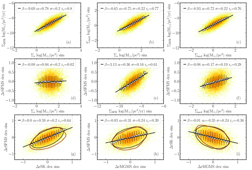
Figure 7: Results of the exploration of a simple simulated dataset comprising 10,000 spatially resolved SF regions following a linear rSFMS ($\alpha=$1, $\beta=$-10) and a linear rMGMS ($\alpha=$1, $\beta=$-1), with $\Sigma_{\rm*}$ distributed randomly around an average value of 10^1.25 M${}_{\odot}/$pc² following a standard normal distribution with a standard deviation of of $\sigma=$0.675 dex. The typical errors corresponding to the observed dataset are simulated by adding random noise to each of the considered parameters, $\Sigma_{\rm*}$ , $\Sigma_{\rm SFR}$ and $\Sigma_{\rm mol}$ , following a simple Gaussian distribution with a standard deviation of 0.20 dex, 0.20 dex and 0.22 dex, respectively. Top panels show the simulated rSFMS (a) and rMGMS (b), together with the recovered rSK (c). Central panels show the residual of the rSFMS, after subtracting the best fitted linear regression, against $\Sigma_{\rm*}$ (d), $\Sigma_{\rm SFR}$ (e) and $\Sigma_{\rm mol}$ (f). Symbols, insets and labels are similar to the ones adopted in Fig. 6. Finally, bottom panels show the distribution of the residuals of the three relations shown in the top panels versus each other: $\Delta$rSFMS vs. $\Delta$rSK (g), $\Delta$rSFMS vs. $\Delta$MGMS (h) and $\Delta$rSK vs. $\Delta$MGMS. Thus, the bottom panels correspond to the same distributions shown in Fig. 5, but for the simulated distributions. To highlight the similarities between both distributions, we include the density contour of the EDGE dataset encircling the 80% of the points shown in the quoted figure (dark-red solid lines), together with the same density contour for the simulated data (black solid line).

It this were correct, however, these results would be totally inconsistent with those shown in the previous section. To understand in more detail the origin of the observed trends between the residuals, we explore their dependence on the original explored parameters: $\Sigma_{\rm*}$ , $\Sigma_{\rm SFR}$ and $\Sigma_{\rm mol}$ . Figure 6 shows the distributions of these residuals against each other. For completeness, we present the comparison of each residual against each parameter, including the independent parameter of the respective relation. Indeed, having removed the primary dependence, it is expected that the residual of each relation does not depend on the corresponding independent parameter (for example, $\Delta$rSFMS should not depend on $\Sigma_{\rm*}$ ). However, as a sanity check, it is important to demonstrate so. If a dependence were found if would mean that the fitted model is not a good representation of the data, retaining some dependence with the independent parameter (e.g., $\Sigma_{\rm*}$ ). In this case any secondary relation could be just an effect of an incomplete removal of the primary one. For example, a residual dependence of $\Delta$rSFMS with $\Sigma_{\rm*}$ would result in a artificial relations with both $\Sigma_{\rm SFR}$ and $\Sigma_{\rm mol}$ as a consequence of the rSFMS and rMGMS relations. Fig. 6 demonstrates that our fitted models removed most of the variation of their independent parameter. For all three residuals ($\Delta$rSFMS, $\Delta$rSK, and $\Delta$rMGMS), the residual correlations with their original independent parameter have a very low correlation coefficient ($r_{c}$ in the $0.03-0.09$ range), and they present a negligible slope ($\alpha\approx-0.08$ to $0.07$) with no significant improvement over the original standard deviation (see Tab. 1). Curiously, the contrary happens with the corresponding dependent parameter in each relation ($\Sigma_{\rm SFR}$ in $\Delta$rSFMS, $\Sigma_{\rm SFR}$ in $\Delta$rSK, and $\Sigma_{\rm mol}$ in $\Delta$rMGMS). In all three cases there is always a weak/moderate correlation ($r_{c}\sim 0.37-0.59$), a non negligible slope ($\alpha\sim$0.3), and a small but measurable decrease in the standard deviation of the residuals that can be as large as $\sim$20%.

This indicates that despite the fact that the linear relations shown in Fig. 2 and Tab. 1 describe the distribution of observed parameters, they cannot describe the distribution of the errors. These errors induce non negligible residuals, once the best fitted relation is subtracted, in both the independent and the dependent parameter and those residuals correlate with each other. The reason is that any deviation from the main relation due to an error induces a residual that depends on this error modulo the slope of the relation, as we will show in the next section. This residual will correlate with the dependent parameter too, since the best fitted relation for the observed parameters minimizes the correlation of the residual of the dependent parameter with the independent one, but it does not minimize the correlation of that residual with the dependent parameter. This reasoning suggest that the described secondary relations shown in Fig. 5 and 6 may not be physical in nature, which we will explore in detail in the next section.

3.4 Are secondary relations physical?

At first glance, the results from the two previous sections seem contradictory since our best fitted models removed most of the dependence with respect to the independent parameters, but their residuals retain a significant dependence on the dependent parameter of the original relation. In order to prove if the reported relations are physical or if they are induced artificially by the individual errors we have performed a set of simple simulations in which we assume that : (1) the three parameters present a set of linear relations between them; (2) there is no real secondary relation. Thus, the residual of any relation between two of the parameters does not depends on the third one; and finally (3) the individual errors are Poissonian and fully independent between the three parameters (i.e., there is no co-variance). Based on these simulations we try to understand how reliable are the recovered parameters from our fitting scheme and if secondary relations may be induced by errors.

In a more mathematical form, let us assume that three datasets ($x$,$y$ and $z$) are described by a set of linear relations:

$$\begin{split}YX:y=a_{xy}x+b_{xy}\\ YZ:y=a_{zy}z+b_{zy}\\ ZX:z=a_{xz}x+b_{xz}\\ \end{split}$$ (8)

if coefficents $a_{ij}$ and $b_{ij}$ (where $i$ and $j$ take the values $x$,$y$ or $z$, for $i\neq j$) are perfectly well determined, then the residuals of the three relations ($\Delta YX$, $\Delta YZ$ ,$\Delta ZX$) should be zero by construction. However, in the presence of noise, this is not true. Let’s assume that the three datasets are measured in a fully indepedent way. That is, the errors in the measurements are not correlated in any way. In this case, the observed datasets would not be $x$, $y$ and $z$, but:

$$\begin{split}x_{obs}=x+e_{x},\\ y_{obs}=y+e_{y},\\ z_{obs}=z+e_{z},\\ \end{split}$$ (9)

where $e_{i}$ is the error of variable $i$ (an $e_{j}$ is totally independent of $e_{i}$, or any $i\neq j$). In this case the residuals of the relations would be:

$$\begin{split}\Delta YX_{obs}=e_{y}-a_{xy}e_{x},\\ \Delta YZ_{obs}=e_{y}-a_{zy}e_{y},\\ \Delta ZX_{obs}=e_{z}-a_{xz}e_{x},\\ \end{split}$$ (10)

for a perfect determination of the coefficients $a_{ij}$ and $b_{ij}$. If not, a term $e_{b,ij}$+$e_{a,ij}i$ need be subtracted from each equation, to account for the error in the derivation of the coefficients (where $e_{b}$ corresponds to the error in the intercept and $e_{a}$ to the error in the slope). So far we consider negligible those errors for clarity. In this case, it is possible to find correlations (or their absence) between the residuals and the relations and the dependent (or independent) parameters and among the residuals themselves under certain circumstances. It is out of the scope of the current exploration to cover all the possible combinations, which are regulated mostly by (i) the range of values covered by each parameter (characterized by its standard deviation around the mean value $\sigma_{i}$), relative to the error of the considered parameter ($e_{i}$); (ii) the comparison between the errors among the different parameters; and (iii) the slope of the three relations among them ($a_{ij}$). If $\sigma_{i}$ is not orders of magnitude larger than $e_{i}$, and $a_{ij}$ is near one in the three cases, it is expected both a correlation between the residuals and the dependent parameter (since they both includes the term $e_{y}$ or $e_{z}$), and among the residuals themselves (with $\Delta YX$ and $\Delta YZ$ positively correlated due to the presence of $e_{y}$ in both of them, and $\Delta YZ$ and $\Delta ZX$ anti-correlating, since the first depends on $-a_{zy}\,e_{z}$, and the second in $e_{z}$). The strength of each correlation would depend on the actual values of $\sigma_{i}$, $e_{i}$ and $a_{ij}$, and the best simplest way to assess them is through a simulation. A comparison between these induced correlations and the observed relations would establish the physical origin (or not) of the later ones.

For the current exploration, we identify the three parameters ($x$, $y$, and $z$) with $\Sigma_{\rm*}$ , $\Sigma_{\rm SFR}$ , $\Sigma_{\rm mol}$ , in logarithmic scale. We adopt a typical $\sigma_{x}=$0.5 dex for the current dataset, and a typical error of $e_{i}=$0.26 dex, generating a dataset of 10,000 simulated values (per parameter) . The simulated values follow the relations described in Eq. 8, assuming as intercepts ($b_{rSFMS,YX}$=-10.0 dex $b_{rMGMS,ZX}$=-1.0 dex), and values of $\Sigma_{\rm*}$ around 10^1.25 (i.e., $x\sim$1.25$\pm$0.4 dex). These values are adopted to match the observations, although they are unimportant to assess the strength of the error-induced correlations.

Figure 7 presents the main results of this simulation. The upper panels show the simulated distributions between the three considered parameters. The parameters exhibit correlations of similar or slightly higher strength than the observed ones, as our simulated error distribution is very simple and does not include systematic effects, detection limits, correlated noise or non-homogeneous sampling of the distribution as would be expected in real data. For each distribution we repeated the analysis we performed on the observed data in Sec. 3.3 using the same code. This analysis provides the power-law relations between the three parameters, with best fitted values very close to those used to create the simulated data. The standard deviation of the residuals once the best fit relations are subtracted are similar to the ones reported for the observed distributions ($\sigma\sim$0.2 dex). As with the real data (Fig. 6) we explore the possible dependence of the residuals of each simulated relation on each considered parameter. We present in Fig. 7 (central row panels) the results for the simulated $\Delta$rSFMS, as similar distributions are observed in the other two residuals. Similar to the case of the real data, the simulated residuals show no correlation with the independent parameter of the considered relation ($\Sigma_{\rm*}$ , r${}_{c}=$0.03, $\alpha$=-0.01), a weak positive trend with the parameter not involved in the relation ($\Sigma_{\rm mol}$ , r_c=0.24, $\alpha$=0.13), and a clear positive correlation with the dependent parameter of the considered relation (the parameter in the ordinate axis, i.e., $\Sigma_{\rm SFR}$ r_c=0.59, $\alpha$=0.33). The agreement with the observed distributions is very good (compare Fig. 6 and 7). Furthermore, the simulation exhibits clear correlations between the residuals of the three relations: Fig. 7, bottom panel, shows the same distributions shown in Fig. 5, but for the simulated dataset. For comparison purposes we include the contour corresponding to the 80% encircled density of the observed distribution together with that of the simulated ones. The agreement between the shape of the distributions, and the trend and strength of the correlations is remarkable good considering the simplistic nature of the simulation.

Most likely, including the possible correlations between the errors derived from the same dataset (like $\Sigma_{\rm*}$ and $\Sigma_{\rm SFR}$ ), and further fine tuning to match them with the observed distribution in a better way would produce even more similar results. Nonetheless, these simulations are sufficient to demonstrate that the observed secondary trends between the residuals of the explored relations (rSFMS, rSK and rMGMS) and between these residuals and the involved parameters ($\Sigma_{\rm*}$ , $\Sigma_{\rm SFR}$ and $\Sigma_{\rm mol}$ ) are a pure consequence of the noise in the observed datasets. In other words, these relations are most likely a pure mathematical artifact and have no physical origin.

4 Discussion and Conclusions

In this study we have explored the local/resolved and global intensive relations between the surface densities of the stellar mass, star-formation rate and molecular gas mass, using the combined dataset provided by the CALIFA survey and the spatially resolved and aperture integrated CO observations provided by the CARMA and APEX antenna (within the framework of the EDGE collaboration). This exploration comprises the largest dataset of galaxies with spatially resolved molecular gas combined with IFS optical data so far (more than 100 galaxies, and more than 10,000 independent line of sights), and one of the largest dataset of galaxies with aperture matched extimates of the three considered parameters (more than 400 galaxies).

4.1 The connection betweem local and global relations

Using this unique dataset, we have characterized the resolved and global relations between the three described parameters ($\Sigma_{\rm*}$ , $\Sigma_{\rm SFR}$ and $\Sigma_{\rm mol}$ ), for the star-forming regions (galaxies), i.e., the rSFMS, rSK and rMGMS relations (and their corresponding unresolved counterparts). In the case of the resolved properties we confirm that the three relations are well characterized by a single power-law, with a slope near to one, and a small scatter ($\sigma\sim$0.2 dex), as previously described by other authors (Sánchez et al., 2013; Wuyts et al., 2013; Cano-Díaz et al., 2016b; Lin et al., 2019; Ellison et al., 2020a). We show that the intensive global relations follow similar trends as the resolved/local ones, in the three cases, as suggested by previous authors (for each relation Pan et al., 2018; Cano-Díaz et al., 2019; Sánchez, 2020). Indeed, when the distributions of the star-forming regions (and galaxies) are compared in the same parameter space ($\Sigma_{\rm SFR}$ -$\Sigma_{\rm*}$ , $\Sigma_{\rm SFR}$ -$\Sigma_{\rm*}$ and $\Sigma_{\rm mol}$ -$\Sigma_{\rm*}$ ) they are statistically indistinguishable. In other words, they are the same relations. In a recent exploration of this topic, Sánchez et al. (2020) demonstrated that indeed if the resolved regions of galaxies follow a local/resolved relation, the existence of a global one is a pure mathematical derivation from the local one. Using simulations this was already demonstrated for other local relations, like the resolved Mass-Metallicity relation (rMZR or $\Sigma_{\rm*}$ -O/H relation, e.g. Rosales-Ortega et al., 2012). However, this is the first time, to our knowledge, that this is demonstrated for the three explored relations, using such an ample dataset, and using both direct and indirect estimates of the molecular gas via CO observations and dust-to-gas calibrations.

The main implication of the match between the resolved and global intensive relations, and the prevalence of the first ones (Sánchez et al., 2020), is that the main physical processes that regulate star-formation operate at the spatial scales where the resolved ones are found (i.e., at kpc-scales), and not by other processes that affect galaxies as a whole. This does not imply that global processes does not affect the star-formation process (as discussed in Sánchez, 2020). Galaxy interactions among themselves or with the environment, galactic-wide outflows, and the ignition of an active nuclei are some of the global processes that indeed affect the star-formation galaxy wide (Hopkins et al., 2010; Poggianti et al., 2017; Sánchez et al., 2018; Bluck et al., 2019). However, they do not have a direct effect galaxy wide. They affect the whole galaxy through the physical processes that regulate star-formation at the explored resolved scales.

On the other hand, it is known that star-formation happens at much smaller scales than the ones explored here, i.e., the size of molecular clouds (from a few pc to some hundred pc). Newly born stars are created when these clouds fragment and collapse gravitationally. This simple argument was used by Schmidt (1959) to propose a relation between the stellar mass formed in a certain time and the amount of gas in the volume at which the stars are formed. From these arguments, assuming that all new stars are formed in the characteristic free-fall time of the gas Kennicutt (1998b) estimated that the relation between both quantities should follow a power-law of $\sim$1.5. However, this relation cannot be the same as the one we observe at kpc-scales or galaxy wide. The observed relation does not match the formed stellar mass in a free-fall time-scale with the pre-existing gas mass. It relates the average SFR with the average gas mass on much larger scales. The same holds for the rSFMS and rMGMS relations. Indeed, the simple free-fall scheme does not even work at the scale of the molecular clouds too: for an already collapsed molecular cloud in which gas mass has been transformed to stars, the SFR may be the previous gas mass (if all gas is transformed to stars) divided by a characteristic time-scale in which SF happens (with the free-fall time being a good proxy). The emerging relation would connect the previously existing molecular gas mass with the newly created stellar mass (a rMGMS-like relation), or the already happened SFR with both quantities (previously existing or already existing gas and stellar masses, i.e., a rSFMS-like relation). But the existence of those physical relations does not guarantee that the average SFR within a certain time scale and a much larger spatial scale would be related to the current reservoir of molecular gas or the previously formed stellar mass. If that was the case all molecular gas should inevitably collapse at a rate dictated by the free-fall time scale, and all SF should happen in a single burst that consumes all the existing gas.

However, we do not observe this in galaxies or regions within galaxies. Not all the molecular gas is collapsing. Other physical conditions are required for that to happen (e.g. Elmegreen, 1997). The hypothesis explored here is that SFR is somehow regulated by the previously formed stellar content, that prevents or allows the collapse of new molecular clouds. Then, once collapsed, they would individually and locally follow the relation proposed by Kennicutt (1998b) (or a similar one). Therefore, this relation is diluted at kilo-parsec scales by the averaging between regions actually forming and regions still not forming (or with stars already formed) producing a slope in all the observed relations that is shallower ($\sim 1$) than that predicted by the simple free-fall time scheme (1.5). Furthermore, this relation is only valid when averaged over much larger times scales than that of the SF process itself (for instance, the free-fall time scale). This regulation is most probably provided by the SF feedback (including supernovae and stellar wind), as proposed by many different studies (Silk, 1997; Ostriker et al., 2010; Hopkins et al., 2013; Kruijssen et al., 2019). In this case, the typical time scale should correspond to the one required by the characteristic velocity of a stellar wind ($\sim$10-30 km/s) to propagate through the considered physical scales ($\sim$1kpc). This corresponds to $\sim$30-100 Myr. Numerical simulations indeed show that these are the typical spatial- and time-scales at which a well-defined quasi-steady-state exists in which the energy injected by SFR feedback pressurizes on average the ISM (Kim et al., 2017; Kim & Ostriker, 2018; Semenov et al., 2017; Orr et al., 2018), which we speculate leads to the observed relations. If this is the regulation mechanism, then the considered relations should break at spatial scales on which the observed time-scale for the SFR (measured by H$\alpha$ would correspond to $\sim$4-10 Myr) is not large enough for the wind to propagate through the considered spatial regime. This would correspond to $\sim$40-100 pc, a regime at which the described relations has not been explored well. Indeed, the same numerical simulations indicate that at these smaller spatial- and time-scales the SFR and the properties of the ISM exhibit strong local variations. Observationally it is seen a break-down of the rSK relation at happens somewhere between 80-100 pc (Onodera et al., 2010; Verley et al., 2010; Williams et al., 2018) and 500 pc (Kennicutt et al., 2007; Blanc et al., 2009), which could indicate that additional processes affect the regulation process in different galaxies or environments.

As we show in Sec. 3, the three involved quantities are tightly correlated which each other, describing not only a set of relations between any pair of them (Fig. 2), but also they are tightly correlated in the 3D space formed by themselves (Fig. 3), following a power law. Being unclear which of them is the primary independent parameter, a reasonable conclusion is that a physical quantity that parametrizes the effects of the stellar feedback (e.g. Silk, 1997; Lilly et al., 2013), would be the hidden parameter that explains the three relations simultaneously. Current simulations (e.g. Ostriker et al., 2010) and observations (e.g. Leroy et al., 2008; Sun et al., 2020) suggest that the mid-plane pressure, generated mostly by stellar winds and modulated by the gravitational potential and the gas content, could be the hidden parameter behind the explored relations (e.g. Barrera-Ballesteros et al., 2021a, b).

4.2 Are secondary relations needed?

The second most important result from our exploration is that the dispersion about the best derived relations that characterize the resolved relations (rSFMS, rSK and rMGMS) is totally driven by the errors in the individual parameters (Sec. 3.4). Despite the fact that there are appreciable and (in principle) statistically significant secondary correlations between the residuals of these relations and the explored parameters and among the residuals themselves (Sec. 3), our results indicate that they are not physically driven secondary relations, but a pure mathematical artifact of the covariance between axes driven by individual errors or errors. This result has profound implications, since recent explorations have interpreted these secondary relations as physically drivers for the dispersion (Cano-Díaz et al., 2019; Lin et al., 2019; Ellison et al., 2020d; Ellison et al., 2020a; Colombo et al., 2020), motivated either by the variations in the relative amount of gas ($f_{gas}$, related to $\Delta$rMGMS), changes in the SFE (related to $\Delta$rSK), or even other additional properties (like the morphology). Ellison et al. (2020a) reported variations up to an order of magnitude in all the three relations between different galaxies, what may dominate the scatter in the average relations. In summary, they proposed a non-universality of these kpc-scale relations, in the same line of the results by Vulcani et al. (2019).

On the contrary, our results suggest that so far an additional physical driver may not be required to explain the dispersion, which is fully attributable to the errors in the individual parameters. This does not mean that certain regions (and galaxies) do not depart from these relations because of physical reasons. Galaxies/regions with extreme SFE (e.g., Starburst, ULIRGS), would be clearly above the rSFMS and rSK relations (e.g. Ellison et al., 2020c), and on the contrary, galaxies/regions with low $f_{gas}$ would be well below the rSFMS and the rMGMS relations (e.g. Saintonge et al., 2016; Calette et al., 2018; Sánchez et al., 2018; Sánchez et al., 2020). Consequently, earlier-type galaxies (and regions within them), with lower $f_{gas}$ would depart from the corresponding relations. However, this corresponds to regions/galaxies that depart from the observed trends, and not to galaxies well represented by those trends. This was recently discussed in Colombo et al. (2020), where there is a clear different trend with SFE and $f_{gas}$ for galaxies within the SFMS and SK relations (that we now understand are driven by errors) and for galaxies departing from those relations (where the effect is most probably physical).

4.3 Main caveats to our results

Despite the fact that our sample is larger in number of galaxies, and it comprises a much larger number of independent resolved LoS than most of the previously studied ones, the dataset is not free of biases and potential problems. First, our physical spatial resolution ($\sim$ 1.3 kpc) is not good enough to distinguish individual star-forming regions (even giant H ii regions), and certainly it is not good enough to perform an optimal separation between different ionizing sources (e.g., the diffuse Lacerda et al., 2018; Espinosa-Ponce et al., 2020). Therefore, a fraction of the reported dispersion could be due to mixing between regions with different ionizations, and different SF regions. However, following our primary result, the scaling relations seem to have the same characteristic shape (and dispersion) at any physical scale within galaxies (larger than the smaller sampled scale). Therefore, the relatively coarse spatial resolution should not have a significant/strong effect above 500 pc. Obviously, exploring these relations at higher/better physical resolution would improve our understanding of them (e.g. Schruba et al., 2011; Kruijssen & Longmore, 2014), in particular to determine at which scale the relations are expected to break (demonstrating the hypothesis that they are statistical relations , discussed before), and limit the effect of mixing on the accuracy of the estimated parameters which produces an increase of the observational uncertainties.

Second, the EDGE sub-sample, which we use to explore the resolved relations, is still biased towards late-type galaxies in comparison with the CALIFA and APEX sub-samples. Furthermore, it has a relatively shallow depth. Therefore, although it represents a clear improvement over other samples and datasets it may need to be further improved to properly span the parameter space, for example to break the scaling relations by morphology, or to explore in detail the loci of retired regions in the considered diagrams (Fig. 2). Because of this we cannot be totally conclusive. Note, however, that many of the studies regarding the physical drivers of the dispersion around the explored relations base their analyzes on datasets with even stronger sample biases (see the comparison in Fig. 1). In any case, observations of the CALIFA sample with ALMA would be key to improve our understanding of these relations: the CALIFA IFS data are the only ones that span a very large and uniform sample of galaxies with coverage out to 2.5 R_e that is well-matched to the field-of-view of ALMA.

4.4 Summary of the conclusions

Based on the analysis presented in this study we conclude that:

• The intensive form of global and local relations among $\Sigma_{\rm SFR}$ , $\Sigma_{\rm*}$ and $\Sigma_{\rm mol}$ are essentially the same relations, following a set of power-law with the same slopes and zero-points, when expressed in the same units.

• These relations hold at very different scales, from galaxy wide, to scales involving a fraction of the galaxies ($\sim$1/3 of the galaxies), to kiloparsec scales.

• They are expected to break at lower scales (100-500 pc), highlighting their statistical nature, what indicate that some-kind of self-regulation process that happens at kiloparsec scales is behind those relations.

• The three explored parameters ($\Sigma_{\rm SFR}$ , $\Sigma_{\rm*}$ and $\Sigma_{\rm mol}$ ) follow a line (or cylinder) in the three dimensional space, with the relations between each pair of them (known as rSFMS, rSK and rMGMS) just projections of that relation.

• The scatter around this relation (and its projection) is fully dominated by individual errors, without the need of a secondary relation with one of the parameters when the relation between the other two is removed.

Finally, we highlight the importance of understanding the effects of axis covariance and uncertainties in the exploration of possible relations of the residuals of primary relations. An approach such as the one outlined in this study need be applied in future explorations, and to revisit claims of secondary relations with the required detail. In future explorations with the current dataset we will try to understand the underlying nature of the physical parameters driving the described relations (Barrera-Ballesteros et al., 2021b), and the causes of the halting of the star-formation in retired regions in galaxies.

Data Availability

The data used in this article consist of the publicly available DR3 of the CALIFA survey as well as extended surveys such as PISCO. CALIFA DR3 data cubes can be accessed at https://califaserv.caha.es/CALIFA_WEB/public_html/?q=content/califa-3rd-data-release, with direct access to the V500 version used in this article available at ftp://ftp.caha.es/CALIFA/reduced/V500/reduced_v2.2/.

The EDGE CO datacubes are publicly available at https://www.astro.umd.edu/EDGE/.

The APEX data will be delivered in a forthcoming article (Colombo et al. in prep.). A preliminary description of the data is included in (Colombo et al., 2020)

References

- Aguado et al. (2019) Aguado D. S., et al., 2019, ApJS, 240, 23
- Astropy Collaboration et al. (2013) Astropy Collaboration et al., 2013, A&A, 558, A33
- Astropy Collaboration et al. (2018) Astropy Collaboration et al., 2018, aj, 156, 123
- Baldwin et al. (1981) Baldwin J. A., Phillips M. M., Terlevich R., 1981, PASP, 93, 5