Machine-learning interatomic potentials for materials science

Abstract

Large-scale atomistic computer simulations of materials rely on interatomic potentials providing computationally efficient predictions of energy and Newtonian forces. Traditional potentials have served in this capacity for over three decades. Recently, a new class of potentials has emerged, which is based on a radically different philosophy. The new potentials are constructed using machine-learning (ML) methods and a massive reference database generated by quantum-mechanical calculations. While the traditional potentials are derived from physical insights into the nature of chemical bonding, the ML potentials utilize a high-dimensional mathematical regression to interpolate between the reference energies. We review the current status of the interatomic potential field, comparing the strengths and weaknesses of the traditional and ML potentials. A third class of potentials is introduced, in which an ML model is coupled with a physics-based potential to improve the transferability to unknown atomic environments. The discussion is focused on potentials intended for materials science applications. Possible future directions in this field are outlined.

Keywords: Atomistic simulation, interatomic potential, machine-learning

1 Introduction

Atomic-scale computer simulations of materials constitute a critical component of the multiscale materials modeling paradigm [1, 2, 3]. They equip researchers with an effective tool for gaining fundamental insights into microscopic mechanisms of processes occurring in materials while also providing quantitative input to mesoscale and continuum models. Modern molecular dynamics (MD) and Monte Carlo (MC) simulations span length scales from a single atom to $\sim 10^{2}$ nm and time scales up to $\sim 10^{2}$ ns. Access to these length and time scales is enabled by classical interatomic potentials (also known as classical force fields), whose role is to predict the energy and classical forces acting on the atoms for any given atomic configuration. Computations with classical potentials are fast and scale linearly with the number of atoms, making them the critical ingredient for all large-scale atomistic simulations. The accuracy and reliability of atomistic simulations often depends on the quality of the interatomic potentials.

The history of quantitative interatomic potentials can probably be counted from the 1980s when the first many-body potentials for metallic systems [4, 5] and bond-order-type potentials for covalent materials [6, 7, 8, 9] were introduced, and their predictive capabilities were demonstrated in several successful applications. Since then, potentials have been developed for most of the chemical elements (for some, several versions are available), for many binary systems, and several ternary and higher-order systems. Many new functional forms of the potentials have been proposed to improve the accuracy of representing the chemical bonding in various classes of materials.

Table 1: Comparison of three classes of interatomic potentials.

	Potential type
	Traditional	ML	Physically-informed ML
Physical foundation	Strong	None	Strong
Number of fitting parameters	$\sim 10$	$\gtrsim 10^{3}$	$\gtrsim 10^{3}$
Computational speed	Very high	Slowera	Slowera
Reference database	Small	Large	Large
Accuracy (interpolation)	Limited	$\sim 1$ meV/atom	$\sim 1$ meV/atom
Transferability (extrapolation)	Reasonable	Poor	Reasonable
Reliance on human expertise	Strong	Weakerb	Weakerb
Extension to chemistries	Challenge	Challenge	Challenge
Specific to class of materials?	Yes	No	No
Systematically improvable?	No	Yes	Yes
Can be made artificial?	Yes	Maybec	Maybec

^a but orders of magnitude faster than straight DFT calculations.

^b Some steps of database selection and training can be partially automatized.

^c Not impossible in principle but we are not aware of attempts.

The quality of the currently available potentials varies widely. Some reach the highest accuracy achievable with the limited number of fitting parameters, while there is a multitude of poor-quality potentials. Some potentials have been employed in hundreds of simulation studies by many groups worldwide, while others were never used outside the original publication. The construction of high-quality potentials heavily relies on human expertise and is considered a borderline between art and science [10, 11]. Infrastructure has been created for the development, testing, standardization, and storage of interatomic potentials, including the NIST Interatomic Potentials Repository [12, 13, 14], the Knowledgebase of Interatomic Models (OpenKim) [15, 16], and potential development tools such as potfit [17, 18, 19], KLIFF [20] and Atomicrex [21].

Over the past decade, a new direction has emerged in this field, wherein the interatomic potentials are constructed by machine-learning (ML) methods, see for example [22, 23, 24, 25, 26, 27] for recent reviews. The idea was initially conceived in the chemistry community in the early 1990s in the effort to improve the accuracy of intermolecular force fields [29, 30]. After two quiet decades, the construction of ML potentials exploded into a powerful new research direction that gained popularity in computational materials science, computational physics, and computational chemistry. In materials science, the emergence and development of the ML potentials can be seen as part of the more general quest for data-driven approaches capable of accelerating the discovery and design of new materials [31, 32, 33, 34, 35, 36, 37, 38, 39, 40]. In simple terms, the basic idea of ML potentials is to forego the physical insights and try to predict the potential energy of the system by numerical interpolation between known reference data (energy, forces and often stresses) generated by quantum-mechanical calculations. This approach signifies a radical departure from the traditional potentials aiming to achieve the same goal by capturing the basic physics of interatomic bonding in the material in question.

The goal of this article is to review the current status and offer the author’s view of the future of the interatomic potential field. Attention will be focused on potentials intended for materials science applications, such as the modeling of microstructure, defects, mechanical and thermal properties, and alloy thermodynamics and kinetics. This excludes the numerous chemical applications, molecular matter, and molecule-surface interaction systems. The reader interested in ML force fields for molecular systems is referred to the recent literature [41, 22, 42, 43, 44]. In terms of the ML methods, we mostly discuss the high-dimensional regression models, which are utilized for the potential training and fall in the category of supervised ML. Classification problems, pattern recognition, clustering, and many other unsupervised learning approaches [31, 33, 34, 35, 36, 38] are also actively used in materials research but lie outside the scope of the article.

The leading theme of the article is the comparison of the traditional and ML potentials. We discuss their strong and weak points, some of which are complementary to each other. A summary of this comparison is presented in Table 1, with a more detailed analysis to follow. After a brief overview of the traditional potentials in section 2, we review the general idea of the ML potentials (section 3.1) followed by a more detailed discussion of the technical aspects, such as the types of regression, the structural descriptors, the reference database construction, and the training process. A summary of the ML potentials is presented in section 3.7. Section 4 introduces the general idea of the physically-informed ML potentials combining the high training accuracy with physics-based transferability. The approach is illustrated by the specific example of physically-informed neural network potentials. Finally, in section 5 we summarize this review and present our view of the history and vision of the future of this field.

2 The traditional interatomic potentials

2.1 What are the potentials, and why do we need them?

The most accurate energy and force calculations are performed by electronic structure methods based on the direct quantum-mechanical treatment of the electrons. Since the density functional theory (DFT) [45, 46] is employed in most of such calculations, we will refer to them for brevity as “DFT calculations”. In addition to the high accuracy (typically, a few meV/atom) and deep physical underpinnings, the DFT calculations can be applied to both elemental and multicomponent systems with nearly equal computational effort. This makes DFT calculations a highly effective tool for a broad exploration of materials chemistry [47, 48, 49]. DFT calculations also provide access to a broad spectrum of physical properties, ranging from mechanical to electronic, magnetic and optical. A major limitation of the DFT calculations is that they are computationally demanding and scale with the number of atoms $N$ as $N^{3}$ or slower. At present, static DFT calculations can only be performed for systems containing a few hundred atoms. Ab initio molecular dynamics (AIMD) can be run for about a hundred picoseconds.

Meanwhile, the intrinsic length and time scales of many materials processes greatly exceed the scales currently accessible by DFT calculations. Examples include plastic deformation, fracture, phase nucleation and growth (including, for example, alloy melting and solidification), and the microstructure evolution by solid-solid interface migration. The modeling of such processes requires access to large collections of atoms and statistical averaging over multiple thermally activated events. Classical interatomic potentials offer a solution by enabling drastically accelerated MD and MC simulations at the price of significantly reduced accuracy. In addition to the accuracy compromise, the classical-mechanical nature of the potential-based simulations excludes any treatment of electric, magnetic or optical properties.

Interatomic potentials parameterize the system’s configuration space and express its potential energy $E$ as a function of the atomic positions (Fig. 1). This function can be represented by a $3N$-dimensional hypersurface called the potential energy surface (PES). Knowing the PES, the forces $\mathbf{F}_{i}=-\partial E/\partial\mathbf{r}_{i}$ acting on individual atoms $i$ can be computed for any atomic configuration ($\mathbf{r}_{i}$ being the position vector of atom $i$). Almost all potentials partition the total energy into energies $E_{i}$ assigned to individual atoms: $E=\sum_{i}E_{i}$. Each atomic energy $E_{i}$ is expressed as a function of the atomic positions $\mathbf{R}_{i}\equiv(\mathbf{r}_{i1},\mathbf{r}_{i2},...,\mathbf{r}_{in_{i}})$ in the vicinity of the atom. The functional form of the potential,

$$E_{i}=\Phi(\mathbf{R}_{i},\mathbf{p}_{i}),$$ (1)

ensures the invariance of the energy under rotations and translations of the coordinate axes and permutations of the atoms. In Eq.(1), $\mathbf{p}_{i}$ is a set of parameters discussed below. The partitioning into atomic energies accelerates the total energy calculation by making it a linear $N$ procedure and enabling parallelization by domain decomposition. We emphasize, however, that this partitioning is only valid for systems with short-range interactions. Long-range Coulomb and dispersive interactions must be added as separate terms and computed by the Ewald summation or similar numerical methods.

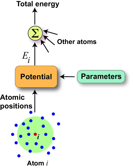
Figure 1: Flowchart of total energy calculations with traditional interatomic potentials. The energy $E_{i}$ of an atom $i$ is computed using atomic coordinates within the cutoff sphere (green) and fixed values of the potential parameters. The atomic energies of all atoms of the system are summed up (symbol $\Sigma$) to obtain the total energy.

2.2 The physical basis of traditional potentials

The distinguishing feature of the traditional potentials is that the potential function $\Phi(\mathbf{R}_{i},\mathbf{p}_{i})$ is based on a physical understanding of interatomic bonding in the material (Table 1). For example, the embedded-atom method (EAM) [4, 5, 50], the modified EAM (MEAM) [51], and the angular-dependent potential (ADP) [52] are specifically designed for metallic systems. The Tersoff [6, 7, 8] and Stillinger-Weber [9] potentials were specifically developed for strongly covalent materials such as silicon and carbon. The charge-optimized many-body (COMB) potentials [53], reactive bond-order (REBO) potentials [54, 10, 55], and reactive force fields (ReaxFF) [56] are most appropriate for molecular systems with chemical reactions. The functional forms of the traditional potentials are diverse and largely incompatible with each other due to the differences in the underlying physical and chemical models specific to the respective classes of materials. This disparity of the functional forms poses a formidable challenge to modeling mixed-bonding and two-phase systems containing metal-ceramic or metal-polymer interfaces.

2.3 Training of traditional potentials

The potential function (1) of the traditional potentials depends on a small number $m$ (usually, 10 to 20) of global (same for all atoms) fitting parameters $\mathbf{p}=(p_{1},...,p_{m})$. These parameters are optimized by training on a database usually composed of experimental data and a relatively small number of DFT energies or forces. The experimental information comes in the form of specific physical properties of the targeted material. Such properties typically include the lattice constant, cohesive energy, elastic constants, point defect formation and migration energies, surface energies, and generalized stacking fault energies. By contrast to the ML potentials discussed later, the traditional potentials are fitted directly to these properties, not the PES. Once optimized, the potential parameters are fixed once and for all and are used for predicting the energy and forces in all atomic configurations encountered during the subsequent simulations. Due to the mathematical simplicity of the potential function, such calculations are computationally fast, easily parallelizable, and provide access to systems containing millions of atoms.

The loss function minimized during the potential training is usually the mean squared deviation of properties from their reference values. These deviations are included with weights assigned to individual properties and playing the role of hyper-parameters. Since the reference database is small, a single training run is computationally fast. However, the potential obtained has to be tested for many physical properties not represented in the training database. Some of the tests, such as computing the melting temperature, require lengthy simulations. The optimization process has a feedback loop in which the hyper-parameters are adjusted by the developer to improve the testing results. This loop is the most critical step of the potentials construction that heavily relies on human decisions and can hardly be automatized. Relationships between the weights of the fitted properties and the accuracy of the tested properties are not apparent. Decisions have to be made based on the developer’s prior experience, intuition, and knowledge of many intricacies of atomistic simulations. The enormous complexity of the property-based optimization and the reliance on expert knowledge make the development of high-quality potentials a long and painful process.

The accepted practice in constructing multicomponent potentials is to preserve the underlying elemental potentials and only fit the parameters of the cross-interaction functions. With this strategy, one elemental potential can be crossed with many others. This property of multicomponent potentials, which we call the “inheritance” of the elemental potentials, helps avoid duplication of potentials and greatly facilitates their standardization and organization in repositories. Nevertheless, the chemical exploration using potentials is much more complicated than with DFT calculations. Each time an element must be added to the system, a new set of cross-interaction functions must be fitted, which requires significant efforts.

2.4 Accuracy and transferability of traditional potentials

Although the construction of traditional potentials is based on physical insights, the underlying physical models are highly approximate and contain few adjustable parameters. As a result, their accuracy is rather limited (Table 1). While some properties are reproduced with decent accuracy, there are many subtle effects (such as specific surface reconstructions or complex dislocation core structures) that are not predicted correctly [60]. Traditional potentials are especially struggling with complex elements such as Si capable of exhibiting both covalent and metallic types of bonding. Carbon is another difficult case due to its bonding complexity and the existence of multiple metastable 3D, 2D, and 1D structures. There are many examples of wrong predictions by traditional potentials and their failures to describe particular properties in particular systems. Nevertheless, many predictions were subsequently confirmed by experiment or DFT calculations. Much of the current knowledge of dislocations, grain boundaries, and other interfaces emerged from potential-based MD and MC simulations performed over the past decades.

Despite the limited accuracy, the traditional potentials often demonstrate reasonably good transferability to atomic configurations lying well outside the training dataset. This important property of traditional potentials is due to the incorporation of basic physics in their functional form (Table 1). As long as the nature of the chemical bonding in the material remains the same as was assumed during the potential construction, the potential should make at least physically meaningful energy predictions for new configurations not represented during the training (Fig. 2a).

2.5 Classification of interatomic potentials

In terms of intended applications, all potentials, regardless of their functional form, can be classified into three categories: general-purpose type, special-purpose type, and artificial.

The general-purpose potentials are trained to reproduce a broad spectrum of physical properties considered most important for the subsequent atomistic simulations. Although the training process targets a particular set of properties, the underlying reference structures must be diverse enough to represent the most typical atomic environments occurring in typical simulations. Once released to the community, a general-purpose potential is used for almost any type of simulation that the user may choose to perform. Most of the atomistic simulations conducted today utilize such off-the-shelf potentials. In addition to the computational speed, the reason for their popularity is their reasonable transferability mentioned above. Even when taken well outside the training domain, the potential may lose much of its accuracy but does not usually generate physically nonsensical results.

Special-purpose potentials are designed for one particular type of simulation. They target a specific application and are not expected to be transferable to other types of simulation. For example, a potential can be specifically trained to reproduce the lattice dynamics and phonon thermal conductivity of a particular element or compound.

The third class is comprised of the so-called artificial (synthetic) potentials. Taking advantage of the property-based training, one can construct a series of artificial potentials with a varying value of a particular physical property (or properties) while keeping other properties unaltered. Simulations with such potentials and comparison with experiments or theory may help the user better understand the impacts of the different physical parameters on a particular process. For example, one can generate a set of face-centered-cubic (FCC) potentials with a varying stacking fault or twin boundary energy with all other properties fixed. Simulation of plastic deformation with these potentials may help disentangle the effects of the fault energies on the deformation modes from other possible effects. As another example, simulations with artificial Al potentials that significantly modified the liquid properties helped the authors [61] to unravel a relationship between the solid-liquid interface mobility and the liquid diffusion coefficient. Artificial potentials are also part of the simulated alchemy approach [62, 63, 64], in which a reversible path between two states is implemented by tampering with the potential. For example, the potential can be modified by small increments (e.g., by the rule of mixtures) to transform one elemental potential into another. Alternatively, some atoms can be slowly removed from the system (made invisible) by gradually dialing down their interactions with the remaining atoms. The free energy difference between the two states of the system can be then computed by the $\lambda$-integration method [62, 65, 66, 67].

We emphasize that the above classification is based on the intended usage of the potential and is common to both traditional and ML potentials. The same functional form can be used to generate a potential for any of the three categories.

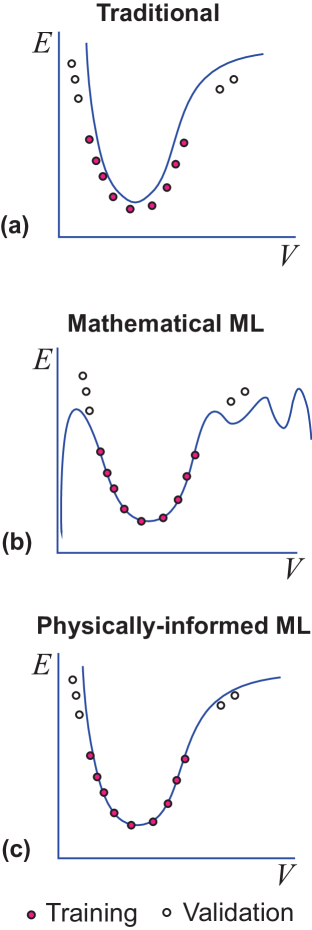
Figure 2: Schematic illustration of accuracy and transferability of (a) traditional (b) mathematical ML and (c) physically-informed ML interatomic potentials. The energy-volume ($E$-$V$) relation for a particular structure obtained by DFT calculations (points) is compared with predictions of the potentials. The points inside and outside the training domain are shown by filled and open circles, respectively.

3 Machine-learning potentials

3.1 The basic idea

While the traditional potentials target a particular set of properties, the ML potentials map the $3N$-dimensional configurational space of the system onto its PES. The latter is represented by a discrete set of DFT energies included in the training dataset. The mapping is implemented by a numerical interpolation algorithm (regression) containing a large number of adjustable parameters. The goal of the training is to optimize the regression parameters to obtain a smooth PES that best interpolates between the reference energies. The energy gradients at the reference points, obtained from the DFT atomic forces, can also be included in the optimization process. Given the large size of the reference database and the high dimensionality of the parameter space, the optimization problem is complex and greatly benefits from the application of ML methods.

Like the traditional potentials, most of the ML potentials are predicated on the locality of atomic interactions and thus partition the total energy $E=\sum_{i}E_{i}$ into atomic energies $E_{i}$. Considering an elemental material to simplify the discussion, the local environment of an atom $i$ is defined by the set of positions $\mathbf{R}_{i}\equiv(\mathbf{r}_{i1},\mathbf{r}_{i2},...,\mathbf{r}_{in})$ of its $n$ neighbors within a cutoff sphere of a radius $r_{c}$ (for a multicomponent system, the chemical identities of the atoms are also considered). The local position vector $\mathbf{R}_{i}$ is mapped onto the local energy by the potential function (1). The total PES is reconstructed by the summation of such local maps. As with the traditional potentials, the locality approximation accelerates the total energy calculation and enables its effective parallelization by the spatial domain decomposition of the system. The locality also justifies using DFT calculations for small supercells to make the energy predictions for large systems. (Efforts to include long-range interactions due, for example, to electrostatic forces have also been published [68, 69, 70].)

The local mapping is implemented in two steps. First, instead of the position vector $\mathbf{R}_{i}$, the local atomic environment is represented by another vector composed of local structural parameters $\mathbf{G}_{i}=(G_{i1},G_{i2},...,G_{iK})$. These parameters are smooth functions of $\mathbf{R}_{i}$ invariant under translations and rotations of the coordinate axes and permutations (relabeling) of the atoms. At the second step, the vector $\mathbf{G}_{i}$ is mapped onto the energy $E_{i}$ by a chosen regression model $\mathcal{R}$. Thus, the atomic energy calculation can be represented by the formula

$$\mathbf{R}_{i}\rightarrow\mathbf{G}_{i}\overset{\mathcal{R}}{\rightarrow}E_{i}$$ (2)

shown diagrammatically in Fig. 3.

The role of the structural descriptors $\mathbf{G}_{i}$ is twofold. First, they ensure the mentioned invariance and smoothness of the PES. The second role of the $\mathbf{G}_{i}$’s is to replace the variable-size position vector $\mathbf{R}_{i}$ (whose length $n$ can vary from one atom to another according to the number of neighbors) by a feature vector of a fixed length $K$. The introduction of a fixed number of local structural descriptors was a crucial step proposed by Behler and Parrinello [71]. Although they initially focused on a single-component system, the general idea of fixing the size of the descriptors was later extended to multicomponent systems [68, 69, 72, 73, 74, 75, 76, 77, 78, 79, 80, 81, 82]. With $K$ fixed, the total energy calculation can be accomplished with a single pre-trained regression $\mathcal{R}$ mapping the $K$-dimensional feature space onto the 1D space of atomic energies. (This explains why the regression symbol $\mathcal{R}$ in Eq.(2) does not carry the index $i$.) The possible regression models $\mathcal{R}$ implementing this mapping will be discussed later.

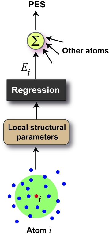
Figure 3: Flowchart of total energy calculations with ML interatomic potentials. The local environment of an atom $i$ within the cutoff sphere (green) is encoded in a set of local structural parameters, which are then mapped onto the energy $E_{i}$ assigned to atom $i$ using a regression model. The summation of the energies of other atoms of the system (symbol $\Sigma$) gives the total energy and thus a point on the PES of the system.

The preceding discussion points to three distinguishing features of ML potentials compared with the traditional potentials (Table 1):

• The reference database is generated by DFT calculations without any experimental input.

• The energy is predicted by purely numerical interpolation of the reference dataset without any physics-based model. The only physical input is the assumption of the locality of the atomic interactions and the invariance of energy under translations, rotations, and permutations of atoms.

• The potential is trained to approximate the PES of the system and not a particular physical property or properties.

In principle, the PES uniquely defines all properties of the system. Its local minima represent stable or metastable structures; the saddle points correspond to energy barriers of thermally activated kinetic processes, such as vacancy jumps or Peierls barriers of dislocations, while the PES curvature controls the elastic constants and phonon dispersion relations. In reality, however, the inevitable deviations of the approximate PES from the theoretical one obtained by DFT calculations cause errors in the predicted physical properties. We will return to the PES versus properties issue later. In the following sections, we briefly review some of the specific steps of the ML potential development.

3.2 The local structural descriptors

The local structural parameters $\mathbf{G}_{i}=(G_{i1},G_{i2},...,G_{iK})$ encode the local environment of every atom $i$ in a fixed number of invariant parameters, often referred to as local fingerprints. As already mentioned, the underlying assumption is that the atomic interactions are short-range, and thus the energy assigned to atom $i$ only depends on its local environment. The total energy is predicted based on the information about all local environments in the system.

The vector $\mathbf{G}_{i}$ is a function of the neighbor positions $\mathbf{R}_{i}$ (and their chemical identities in multicomponent systems). The choice of this function is extremely important and can strongly impact the accuracy of the potential. The general requirement for this function is to capture the local atomic environment most efficiently. The efficiency includes the resolution (different environments must be represented by sufficiently different descriptors), the descriptor size $K$, and the computational cost of its calculation. A more detailed list of expected properties of descriptors can be found in [83]. It is also desirable that the set of descriptors be complete, i.e., capable of exactly reconstructing the local environment (up to symmetry operations) at least in principle. In the absence of completeness, the descriptors can miss certain structural features. On the other hand, an overcomplete set can generate different descriptors for the same structure, resulting in discontinuous behavior of energy predictions. Several representations based on complete basis sets have been proposed [84, 85]. In practice, only two- and and three-body terms are usually utilized. The issues surrounding the incompleteness of such “truncated” representations have been recently investigated [86].

More detailed theoretical analysis and benchmarking of different descriptors can be found in the literature [87, 88, 89, 84, 25, 90, 85, 86, 83]. In practice, different authors use their favorite $\mathbf{G}_{i}$’s, which often perform equally well. Some of the commonly used descriptors include:

Gaussian descriptors. Combinations of two-body and three-body Gaussian functions of interatomic distances and bond angles are multiplied by a smooth cutoff function. A particular case, called the symmetry functions, was proposed by Behler and Parrinello [71], but other functional forms can be equally efficient [23, 88, 91, 92, 93]. It was proposed [91, 92, 93] to express the bond-angle dependence through Legendre polynomials since they form an orthogonal and complete set.

Zernike descriptors. The atomic environment is represented by coefficients (moments) on the basis of Zernike functions [94, 95], which have the advantage of forming an orthogonal basis set and automatically including many-body interactions. Khorshidi et al. [95] demonstrate that the Zernike descriptors are computationally faster than the bispectrum method (see below) and that their derivatives (needed for the force calculations) can be computed more easily.

Moment tensor descriptors [96]. Moment tensors of different ranks are formed by multiplying radial functions by outer products of the position vectors of the neighboring atoms. Rotationally and permutationally invariant descriptors are obtained from contractions of these tensors to produce scalars. These descriptors are used as part of the moment tensor potentials (MTP) [96, 97, 98, 99, 100]. The MTP descriptors form a complete basis set of polynomials if all orders are included. In the recent tests of several ML potentials [25], the MTP potentials have shown the optimal combination of accuracy and computational efficiency.

Smooth overlap of atomic positions (SOAP) [101, 87]. The neighboring atoms are represented by overlapping Gaussian peaks of density, which are expanded in spherical harmonics. The bispectrum descriptors are formed from the expansion coefficients and are rotationally invariant. The SOAP descriptors have proved to be very powerful but computationally slower than the alternatives mentioned above and below. Although designed in tandem with the Gaussian approximation potentials (GAP), they can also be combined with neural networks [95] and other regression models.

Spectral neighbor analysis potential (SNAP) descriptors [102]. The fingerprinting of the environment is somewhat similar to that in the SOAP method. The density peaks corresponding to the neighboring atoms are expanded on the basis of 4D hyper-spherical harmonics. The bispectrum formed by the expansion coefficients provides the local structural descriptors. A multicomponent extension of the method has been recently developed [103].

Atomic cluster expansion (ACE) [84] can be viewed as a generalization of some of the above descriptors. The atomic environment is represented by a set of invariant polynomials of functions forming a complete basis. Each basis function is a product of a radial function and an angular component represented by a spherical harmonic. Linear scaling with the number of neighbors is achieved by transforming the sums products into products of sums (which is also done with the MTP descriptors). The expansion can be applied to multicomponent environments. For atomic clusters, ACE provides a good linear model for energy predictions. For bulk systems, a nonlinear model has been proposed by combining the ACE descriptors with a traditional interatomic potential in the Finnis-Sinclair [50] or any other format. The method has been recently extended to vectorial and tensorial physical properties [105].

Assessing the efficiency of descriptors is challenging since their performance depends on the regression model and the database used for the testing. The benchmarking of different potentials [25] does not shed much light on the descriptors’ performance since they are only responsible for one step in the energy calculation. Onat et al. [83] have recently published a detailed comparison of the sensitivity of eight most popular descriptors to structural perturbations using four different reference datasets.

3.3 The regression models

Several high-dimensional regression models are available for mapping the local environments of atoms onto the PES. The most common choices are the Gaussian process regression [106, 101, 87, 107, 108, 109, 110] (underlying the GAP potentials), the kernel ridge regression [111, 112, 31], the SNAP model [102, 113, 78], the MTP potentials [96], and the artificial neural network (NN) regression [71, 114, 115, 116, 117, 118, 119, 120, 72, 121, 22, 42, 122]. Some of the models (such as SNAP and MTP) are linear, while others are highly nonlinear. They contain a large ($\sim 10^{3}$) number of parameters, which are trained on a DFT database.

We will concentrate the discussion on the NN regression as an example. NNs have the advantage of being very flexible, not affected by any constraints specific to the material system, and being universal approximators [123]. NNs are widely used in materials science and many other areas of science and technology. Thus, the existing experience, methodologies, and even some software packages can be transferred to the potential development field.

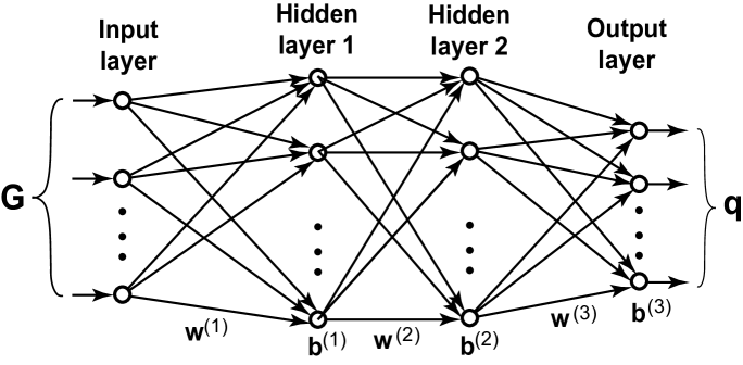
Figure 4: Example of a feed-forward NN containing two hidden layers. $\mathbf{G}$ is the input vector, $\mathbf{q}$ is the output vector. The signals transmitted between the NN nodes (neurons) are transformed by the weight matrices $\mathbf{w}^{(1)}$, $\mathbf{w}^{(2)}$ and $\mathbf{w}^{(3)}$ and the bias vectors $\mathbf{b}^{(1)}$, $\mathbf{b}^{(2)}$ and $\mathbf{b}^{(3)}$.

Most of the NN potentials utilize a simple feed-forward architecture, where the nodes (neurons) are organized in layers. The feature vector is fed into the input layer, the output layer delivers the energy or force, and the hidden layers inserted in between provide additional adjustable parameters and enhance the flexibility of the model (Fig. 4). The output layer consists of just one node for PES fitting, but three more nodes with Cartesian components of the force can be added if force matching is part of the training. Generally, we can consider a feed-forward NN with an architecture $K-k-l...-m$ composed of $M$ layers labeled by an index $n=1,2,...,M$. The input layer ($n=1$) contains $K$ nodes, which receive the input parameters $G_{\eta}$, $\eta=1,2,..,K$. These are multiplied by weights $w_{\eta\nu}^{(1)}$ ($\nu=1,2,...,k$), shifted by biases $b_{\nu}^{(1)}$, and sent as input to the first hidden layer ($n=2$). This layer applies a transfer (activation) function $f^{(2)}(x)$ at each node, producing a set of outputs $t_{\nu}^{(2)}=f^{(2)}(\sum_{\kappa=1}^{\kappa=m}G_{\kappa}w_{\kappa\nu}^{(1)}+b_{\nu}^{(1)})$. They are multiplied by another set of weights $w_{\nu\mu}^{(2)}$ ($\mu=1,2,...,l$), shifted by biases $b_{\mu}^{(2)}$, and the parameters $\sum_{\kappa=1}^{\kappa=l}t_{\kappa}^{(2)}w_{\kappa\mu}^{(2)}+b_{\mu}^{(2)}$ are fed into the next layer with $n=3$, which applies to them its own transfer function $f^{(3)}(x)$, and the process continues. The last layer ($n=M$) does not change its input parameters $t_{\lambda}^{(M)}$ ($\lambda=1,...,m$) and delivers them as the final NN output. The data flow through the NN can be described by the iteration scheme

$$t_{\eta}^{(n)}=f^{(n)}\left(\sum_{\kappa}t_{\kappa}^{(n-1)}w_{\kappa\eta}^{(n-1)}+b_{\eta}^{(n-1)}\right),\quad n=2,3,...,M,$$ (3)

with the initial condition $t_{\eta}^{(1)}=G_{\eta}$ and the final transfer function $f^{(M)}(x)\equiv x$.

Thus, a feed-forward network implements a nested analytical function with the weights $w_{\kappa\eta}^{(n)}$ and biases $b_{\eta}^{(n)}$ as fitting parameters. Typical transfer functions are the sigmoidal function $f(x)=\left(1+e^{-x}\right)^{-1}$ and the hyperbolic tangent $f(x)=\tanh(x)$, but other functions with similar shapes can also be used. The reader is referred to Behler’s paper [119] for an excellent exposition of the NN method, including the exact count of the total number of parameters and comparison of different transfer functions.

Although the NN architecture itself has no physical meaning, it provides hyper-parameters that can be optimized during the training by adding or removing nodes or whole layers. This is usually accomplished by trial and error, but evolutionary algorithms and other architecture search methods have also been proposed. In addition to the feed-forward architectures, convolutional networks and radial basis function NNs have been explored, although mostly for organic molecules [42].

We emphasize again that in all cases, the regression model is little more than a black box with many fitting parameters without any physical significance.

3.4 The training and validation of ML potentials

The regression $\mathcal{R}$ in Eq.(2) depends on a large set of adjustable parameters, which are optimized to best reproduce the input-output pairs from the DFT dataset. The reference DFT data comes in the form of energies $\left\{E_{\textrm{DFT}}^{s}\right\}$ and (often) atomic forces $\left\{\mathbf{F}_{\textrm{DFT}}^{s}\right\}$ and/or stress tensors $\left\{\textsf{$\mathbf{T}$}_{\textrm{DFT}}^{s}\right\}$ for a set of supercells. One specific feature of ML potentials, compared with ML regression problems in other fields, is the absence of one-to-one correspondence between the input feature vectors and the reference energies (respectively, forces or stresses). The potential predicts individual atomic energies, which must be summed over the supercell atoms before comparing the supercell energy $E^{s}$ with the reference value $E_{\textrm{DFT}}^{s}$. It should also be noted that some of the force and stress tensor components can be zero by symmetry and thus useless for the training process.

The simplest form of the loss function minimized during the potential training is

$$\mathcal{E} = \dfrac{1}{N}\sum_{s=1}^{N}\left(\dfrac{E^{s}-E_{\textrm{DFT}}^{s}}{N_{s}}\right)^{2}+\tau_{1}\dfrac{1}{N}\sum_{s=1}^{N}\sum_{\alpha=1}^{3}\left[F_{\alpha}^{s}-\left(F_{\alpha}^{s}\right)_{\textrm{DFT}}\right]^{2}$$ (4)

$$+ \tau_{2}\dfrac{1}{N}\sum_{s=1}^{N}\sum_{\alpha,\beta=1}^{3}\left[T_{\alpha\beta}^{s}-\left(T_{\alpha\beta}^{s}\right)_{\textrm{DFT}}\right]^{2}+\tau_{3}\dfrac{1}{L}\sum_{\kappa=1}^{L}\left|p_{\kappa}\right|^{2}.$$

Here, $N_{s}$ is the number of atoms in supercell $s$, $N$ is the total number of supercells in the database, $L$ is the number of fitting parameters, and $\tau_{1}$, $\tau_{2}$ and $\tau_{3}$ are adjustable coefficients treated as hyper-parameters. The first three terms in the right-hand side represent the mean-square error of fitting. Some authors write the first term as the mean-square error of the supercell energy, not the per-atom energy as in Eq.(4). The last term in Eq.(4) is added for regularization purposes to ensure that the parameters remain sufficiently small for smooth interpolation. Some ML potentials do not require explicit optimization: the parameters are obtained by matrix inversion or similar algebraic operations. In all cases, however, this step must be repeated multiple times to optimize the hyper-parameters.

Once the final values of the potential parameters are established, they are fixed and become part of the definition of the ML potential, just like with the traditional potentials. It is expected that the potential will make accurate energy and force predictions for new configurations by interpolating between the DFT points.

Several optimization algorithms are used, the most common of them being the backpropagation (steepest descent method), the Levenberg-Marquardt, the Davidon-Fletcher-Powell (DFP), and the Broyden–Fletcher–Goldfarb–Shanno (BFGS) unconstrained optimization algorithms [124, 125]. The loss function has a rugged terrain with numerous dimples and wrinkles; hence the gradient methods are easily trapped in local minima. Numerous restarts from different initial guesses are usually required to reach a deeper minimum. Some developers start the training with a global search using, for example, an evolutionary algorithm to avoid the traps, followed by a gradient-based minimization. Because of the large size of the reference database, the training is often performed in a batch mode: the model is optimized on relatively small subsets, selected from the full database at random or by a chosen rotation rule until each configuration is exposed multiple times. The precision of training is measured by either the root-mean-square error (RMSE) or mean absolute error (MAE).

Many strategies have been developed to avoid underfitting or overfitting of the database. The overfitting is especially dangerous as it produces oscillations between the reference points that degrade the predictive capability of the potential. The common practice is to monitor the error of predictions on a small validation set excluded from the training dataset. The divergence between the training and validation errors signals the onset of overfitting. The $k$-fold cross-validation and other validation methods are also applied to test the potentials for overfitting.

Given that the regression models depend on thousands of adjustable parameters and offer enormous flexibility in fitting the reference database, it is hardly surprising that most ML potentials readily achieve the training accuracy of several meV/atom. We emphasize, however, that this high accuracy is achieved by purely numerical interpolation. Predicting the energies of new atomic configurations significantly different from those included in the training database requires extrapolation. Being a purely numerical procedure, the extrapolation can produce unpredictable and often meaningless results (Fig. 2b).

3.5 The reference database

The reference database typically contains $\sim 10^{3}$ to $10^{4}$ supercells with energies, forces, and (often) stresses obtained by routine quantum-mechanical (usually, high-throughput DFT) calculations. Either static structures or snapshots of AIMD trajectories (or both) can be included. Alternatively, the structures can be generated by MD simulations with a current version of the potential, followed by the energy (force and/or stress) calculations by DFT. While there are several schools of thought about the most effective procedure for assembling the database, the consensus is that it should be as diverse as possible and adequately represent the configurations most relevant to the intended applications. Preference is usually given to low-energy configurations, but non-equilibrium structures are also included to represent transition states and cover a broader domain in the configuration space.

There are diverging opinions about the role of human expertise in the ML potential development (as in many other fields of science and technology). One approach is to judiciously select a set of reference structures deemed to be most relevant to the targeted applications. For example, since metals are usually studied for mechanical behavior, structures representing defects are given preference, especially dislocations, twin boundaries, stacking faults, and grain boundaries. Several alternate crystal structures, deformation paths between them, and the liquid phase are also included to expand the configuration domain. On the other hand, properties such as the Grueneisen parameter or the phononic thermal conductivity are considered less important and are rarely even checked. For a covalent material, such as silicon, the potential can be expected to reproduce the thermal conductivity, along with various alternate structures (especially liquid and amorphous) and defects (especially surfaces and the crack tip). For potentials intended for a more specific application, the database will be even more specialized. Assembling such handcrafted datasets requires a fair amount of decision-making based on the developer’s expert knowledge and physical intuition. The reliance on human expertise is even more significant in developing binary and multicomponent potentials intended for a broad range of metallurgical applications [76, 126]. On the downside, a hand-picked database may contain many near-repeat or uninformative local environments that contribute little to the accuracy of the final product.

With this approach, the development of an ML potential becomes similar to that of traditional potentials. In fact, for ML potentials, the situation is more complicated because the training process reproduces the PES and not directly the properties. While theoretically, the PES uniquely defines the properties, in practice, even a tightly fit PES does not automatically guarantee accurate predictions of properties. Experience shows that if a set of potentials is trained on the same database to the same RMSE error (say, 3-5 meV/atom) starting from different initial conditions, such potentials often predict significantly different values of the properties. Additional efforts are required to select a potential with the best combination of properties by testing multiple versions. This adds a human-controlled feedback loop to the training process since the notion of a “best combination” is difficult to express by an algorithm. One way to improve a particular property is to add more reference structures controlling this property. For some properties, this is straightforward. For example, the inclusion of additional supercells containing a vacancy or a particular surface may ensure a more accurate vacancy (respectively, surface) formation energy. For other properties, such as the melting temperature, the connection is less direct and more difficult to control.

Alternatively, algorithms have been proposed for generating the reference database with little or no human intervention. In most cases, the database construction and the potential training become part of one and the same “active learning” process [128, 129, 107, 97, 110, 130, 81, 131, 132, 133]. In a typical scenario, a preliminary version of the potential is trained on an initial DFT database. An MD simulation is performed with this potential until configurations are encountered that are sufficiently different from the known ones, signaling that the simulation ran into a poorly represented region of the configuration space. Different novelty criteria have been proposed to detect the point where the simulation drifts outside the reference domain. The “unknown” configurations are then added to the database, and their DFT energies (forces/stresses) are computed either offline or on-the-fly. The training is continued on the expanded database, and the updated potential is used to continue the MD simulation. The iterations are repeated until self-consistency is reached, i.e., when no new configurations are discovered within a reasonable MD time. The MD simulation can be replaced by random structure searches, in which multiple randomized structures are quenched to find local energy minima. Various other algorithms have been devised for configuration space exploration and training-testing strategies.

Arguably, the advantage of the active learning approaches is the ability to automatically generate the most economical reference database for achieving the desired training accuracy and self-consistent behavior of the final potential. On the other hand, the configuration domain covered by the potential depends on the chosen MD simulation protocol (ensemble, temperatures, densities) or, respectively, on the chosen algorithm for the generation and testing of the new structures. The performance of the potential outside this domain remains uncontrollable. Furthermore, the previous comments about the PES approximation versus the property predictions are relevant to the present case as well. Automatically achieving a desired accuracy of training does not automatically guarantee that the physical property predictions will be accurate enough for practical applications of the potential. Automation is possible and makes sense for surrogate models and some special-purpose potentials. However, a fully automated generation of a general-purpose potential does not seem to be a reasonable expectation.

3.6 ML potential software

Several software packages have been developed for the ML potential generation and simulations. Some are stand-alone packages, others are interfaced with the Large-scale Atomic/Molecular Massively Parallel Simulator (LAMMPS) [134], the Vienna Ab Initio Simulation Package (VASP) [135, 136], or other popular software. In this highly dynamic field, several new packages are released every year. A few examples are given below in no particular order and without any claim of completeness.

ASE (Atomistic Simulation Environment) [137, 138] offers a set of Python tools for setting up, manipulating, running, visualizing, and analyzing atomistic simulations. The environment is linked to simulation software such as LAMMPS, and to DFT packages such as VASP and Quantum Espresso [139]. It provides an excellent platform for DFT database generation and ML potential testing.

Amp (Atomistic Machine-learning Package) [95, 140] is somewhat similar to ASE and additionally contains modules for ML potential training using an assortment of descriptors and optimization algorithms. The focus is on NN potentials, but other user-defined regression models are also accepted. As an example, Amp was applied to develop a quaternary potential for H and CO on a Mo surface [95].

N2P2 (Neural Network Potential Package) [141] provides a repository and tools for the training of Behler-Parrinello type [71] NN potentials and calculation of energies and forces using such potentials. It also contains components needed for running MD simulations with LAMMPS.

Aenet (Atomic Energy Network) [73, 74, 44, 142]. Software package for the training and usage of Behler-Parrinello type [71] NN potentials. Modules for the energy and force calculations with the potentials are also included.

MLIP (Machine Learning Interatomic Potentials) [100, 143] package constructs MTP potentials [96, 97, 80, 100] (including multicomponent potentials [80]) by the active learning approach.

KLIFF (KIM-based Learning-Integrated Fitting Framework) is a package intended for the development of both traditional and NN interatomic potentials. The package is linked to the OpenKIM project [16], and through it, to a large interatomic potential repository and LAMMPS simulations.

MAISE (Module for ab initio structure evolution) [144] is a package for automated generation of NN (Behler-Parrinello type [71]) potentials for global structure optimization. The DFT database is generated automatically by an evolutionary structure sampling procedure.

3.7 Discussion of ML potentials

The distinguishing features of the ML potentials compared with the traditional potentials are summarized in Table 1. When properly trained, an ML potential can predict the energy and forces with nearly DFT accuracy, provided the atomic configuration bears enough similarity with some of the known configurations from the training database. The high accuracy is achieved by numerical interpolation using a high-dimensional regression model trained on a massive DFT database. The regression maps the local atomic environments, encoded in local structural parameters (fingerprints), onto the PES of the material. By contrast to the traditional potentials, which aim to reproduce a particular set of physical properties, ML potentials approximate the PES (actually, only some part of it), with the expectation that accurate values of physical properties will follow. Another crucial difference is that the ML potentials are not based on any physical considerations. The fingerprints and the regression only respect the locality of atomic interactions and the invariance of energy under translations, rotations, and relabeling of atoms but are otherwise devoid of any physical significance. Accordingly, the ML potential are sometimes called “mathematical” or “non-physical” [22].

Freedom from physics is a double-edged sword. ML potentials are not specific to any particular class of materials. A potential for almost any material can be developed with the same model, same software, and a comparable amount of computational effort regardless of the type of chemical bonding. On the other hand, ML potentials are powerful numerical interpolators but poor extrapolators. The energy/force predictions for less familiar atomic environments are based on a purely mathematical extrapolation procedure whose results are unpredictable and often physically meaningless. Special efforts are required to keep the simulations within or close to the configuration domain on which the potential was trained.

Given the limited transferability, there are two approaches to utilizing the ML potentials. One is to develop a special-purpose potential for a particular task without claiming any broader applicability. The approach exploits the ML potentials’ high accuracy and computational efficiency (compared to DFT) while keeping the simulation in the interpolation regime. One recent example is developing a GAP Si potential specifically designed for phonon properties and thermal conductivity calculations, including the effect of vacancies [145]. Similarly, a deep NN potential was constructed to calculate the vacancy formation free energy in Al as a function of temperature [146]. Another excellent example of using a special-purpose potential (deep NN in this case) is the recent study of the nucleation of crystalline Si from the liquid phase [147].

The second approach is to assemble a large and highly diverse reference database covering as broad a configuration domain as possible, including atomic environments that (1) typically occur in atomistic simulations, and (2) are most relevant to the set of physical properties expected to be reproduced by potentials. Simulations with a potential trained on this database will then occur predominantly in the interpolation mode. Theoretically, there is still a chance that the simulation will wander away to unexplored territory or will be trapped in a gap (dark pocket) inside the reference domain. Nevertheless, some of the recent potentials developed with this approach, such as the GAP potentials for Si [109] and C [148], do reproduce an incredibly broad spectrum of physical properties with high accuracy. Based on the broad applicability, the developers place these potentials in the general-purpose category.

Another usage of ML potentials is to provide surrogate models to accelerate DFT calculations. This approach has been especially effective in the area of crystal structure searches [149, 150, 151, 79, 98] combined with active learning by either structure relaxations [98, 80] or evolutionary algorithms [152, 144]. The potential is constructed as part of the structure search and accelerates the search by orders of magnitude compared to high-throughput DFT calculations. In some cases, stable binary or ternary structures have been revealed that were missed by DFT searches. Acceleration of DFT calculations by on-the-fly constructed ML potentials has been proposed for several other applications, such as the melting temperature calculations [127]. In all such cases, the ML potential only plays the role of a temporary construction not intended for independent applications.

4 Physically-informed machine-learning potentials

As discussed in the previous sections, many of the strengths and weaknesses of the traditional and ML potentials are complementary to each other (Table 1). A new direction has recently emerged, aiming to strike a golden compromise between the two by taking the best from both worlds. This goal can be achieved by choosing a general enough form on a physics-based interatomic potential and letting a ML regression predict its parameters according to each atom’s local environment. In contrast to Eq.(2) describing a mathematical ML potential, the formula of a physically-informed ML potential is

$$\mathbf{R}_{i}\rightarrow\mathbf{G}_{i}\overset{\mathcal{R}}{\rightarrow}\mathbf{p}_{i}\overset{\Phi}{\rightarrow}E_{i},$$ (5)

see the flowchart in Fig. 5. Instead of directly predicting the atomic energy $E_{i}$, the regression $\mathcal{R}$ outputs a set of potential parameters $\mathbf{p}_{i}$ most appropriate for the environment of the particular atom $i$. The atomic energy $E_{i}$ is then computed with the interatomic potential $\Phi(\mathbf{R}_{i},\mathbf{p}_{i})$. In other words, the regression output is “piped” through a model whose functional form ensures that the energy predictions are physically meaningful. Extrapolation to new environments is now guided by the physics embodied in the interatomic potential rather than a purely mathematical procedure.

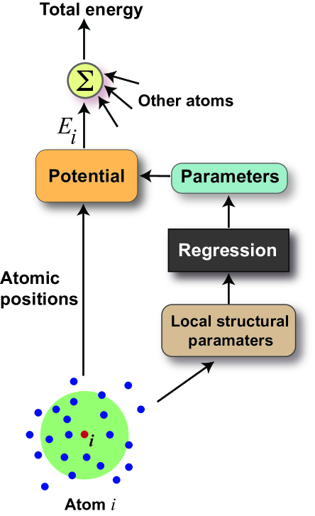
Figure 5: Flowchart of the total energy calculation with a physically-informed ML interatomic potential. The local environment of an atom $i$ within the cutoff sphere (green) is encoded in a set of local structural parameters, which are then mapped onto a set of parameters of a physics-based interatomic potential. These parameters and the local atomic coordinates are used to compute the energy $E_{i}$ assigned to atom $i$. The summation of the energies of other atoms of the system (symbol $\Sigma$) gives the total energy and thus a point on the PES of the system.

Any model eventually fails. Physically-informed ML potentials can also produce unphysical results when taken too far away from the familiar territory. However, the physics-guided extrapolation is likely to expand the potential’s reliability domain compared with purely mathematical models (Fig. 2c).

This general idea can be realized with any regression method and any suitable interatomic potential. The recently developed physically-informed neural network (PINN) method [91] relies on a NN regression and an analytical bond-order potential (BOP) whose functional form is general enough to apply to both metals and nonmetals. A detailed description of the BOP potential can be found in Appendix B. In short, the potential captures pairwise repulsion and attraction of atoms, the bond-order effect (bond weakening with the number of bonds), angular dependence of the bond energies, screening of bonds by surrounding atoms, and the promotion energy. The interactions are limited to a coordination sphere with a smooth cutoff. The local atomic environments are represented by Gaussian descriptors specified in Appendix C, but we emphasize that other choices of the descriptors are equally possible.

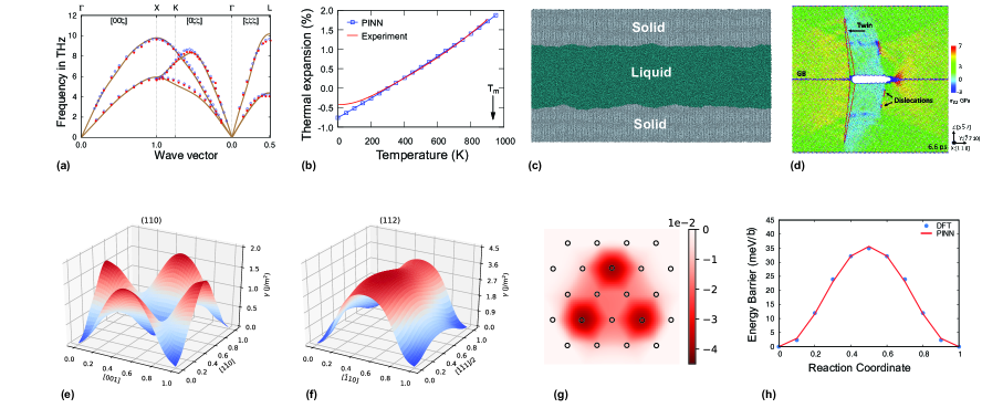
Figure 6: Examples of properties calculated with the PINN potentials for (a-d) Al [92] and (e-h) Ta [93]. (a) Phonon dispersion relations computed with the PINN potential (curves) compared with experimental data (points). (b) Linear thermal expansion relative to room temperature predicted by the PINN potential (points) compared with experiment (curve). (c) Simulation block used for computing the solid-liquid interface tension by the capillary fluctuation method. (d) MD simulation of crack nucleation and growth on a grain boundary. (e,f) $\gamma$-surfaces in body-centered cubic Ta on (110) and (112) planes, respectively. (g) Nye tensor plot of the core structure of the $\frac{1}{2}\left\langle 111\right\rangle$ screw dislocation in Ta predicted by the PINN potential. (h) Peierls barrier of the $\frac{1}{2}\left\langle 111\right\rangle$ screw dislocation predicted by the PINN potential (lines) in comparison with DFT calculations (points).

The original PINN formulation [91] was recently improved [92, 93] by introducing a global version of the BOP potential trained on the entire reference database. After the training, the optimized parameters $\mathbf{p}^{0}=(p_{i1}^{0},...,p_{im}^{0})$ are fixed and become part of the potential definition. Since this parameter set is relatively small ($m\sim 10$), the error of fitting is usually on the order of $10^{2}$ meV/atom. The role of the NN is to add to $\mathbf{p}^{0}$ a set of local “perturbations” $\delta\mathbf{p}_{i}=(\delta p_{i1},...,\delta p_{im})$. The final parameter set $\mathbf{p}_{i}=\mathbf{p}^{0}+\delta\mathbf{p}_{i}$ is then used to predict the atomic energy $E_{i}=\Phi(\mathbf{R}_{i},\mathbf{p}^{0}+\delta\mathbf{p}_{i})$. The magnitudes of the perturbations are kept as small as possible. Their goal is to achieve the DFT level of accuracy of the training. In this model, the energy predictions are largely guided by the global BOP potential $\Phi(\mathbf{R}_{i},\mathbf{p}^{0})$ ensuring a smooth and physically meaningful extrapolation outside the training domain. This scheme has been shown [92, 93] to significantly improve the transferability without compromising the accuracy or increasing the computational cost compared with the original formulation [91].

General-purpose PINN potentials have been constructed for Al [91, 92] and Ta [93], with several other potentials being currently developed. Both the Al and Ta potentials accurately describe a broad spectrum of properties of these metals, including the mechanical and thermal properties most relevant to materials science applications. A select set of examples is given in Fig. 6. A multicomponent version of PINN has been formulated and tested, and is currently being used to develop binary potentials. The computational efficiency of the PINN Al potential has been evaluated [92]. Although the specific numbers depend on the computational software, hardware, and the type of tests, as a general guide, the PINN potential is two orders of magnitude slower than the EAM Al potential [153]. The computational overhead due to the BOP potential is about 25 % of the total time. Considering that ML potentials are orders of magnitude faster than straight DFT calculations, this modest overhead can be considered a small price for the improved transferability.

The general idea of incorporating physics into ML models was explored by several authors in the past. Skinner and Broughton [28] demonstrated that artificial NNs can be used to construct Lennard-Jones and Stilliger-Weber potentials. Other authors developed ReaxFF, BOP, and other traditional potentials by generating a massive DFT database and applying training algorithms adapted from the ML field [154, 155]. Drautz’s ACE potentials [84, 105] are based on a physics-motivated and physically interpretable cluster expansion containing a set of adjustable parameters. While we classify the ACE potentials as traditional, they include some features of ML potentials, such as local structural descriptors and the parameter optimization on a large DFT database. On the other hand, there is a recent trend to include physics-inspired terms in mathematical ML potentials. Glielmo et al. [156] described a construction of $n$-body Gaussian process kernels that capture the $n$-body nature of atomic interactions in physical systems. Additional analytical terms mimicking either short-range pairwise repulsion or long-range van der Waals interactions are included in recent versions of GAP potentials [109, 148]. The parameters describing such terms are fitted separately from the GAP part and then subtracted from the total energy during the training. Perhaps the closest to the PINN model was the work by Malshe et al. [157], who constructed a Tersoff potential for the Si₅ cluster in which the potential parameters were controlled by a pre-trained NN. In their model, the potential parameters were not fixed but varied in the course of MD simulations according to the instantaneous atomic positions.

The physically-informed ML potentials, of which PINN one an example, do not simply fill the gap between the classical and ML potentials but build upon both to create a new and distinct class of interatomic potentials. Like traditional potentials, they adopt an atomic interaction model explicitly describing diverse physical effects, such as the many-body character of interactions, the bond-order effect, and the bond screening by neighbors. (In the future, more effects can be added, such as magnetism.) By contrast to the traditional potentials, the parameters of the physically-informed ML potentials are dynamic: they are locally adjusted during the simulation in response to the ever-changing local atomic environments. At the same time, potentials of this class have the descriptor-regressor structure shared by all ML potentials and are trained on a DFT database using the statistical learning methods.

5 Summary and outlook

ML potentials have emerged as a powerful new tool for materials modeling and new materials discovery. When used within the boundaries of validity, an ML potential can predict the energy and atomic forces with nearly DFT accuracy but orders of magnitude faster. The computational time scales linearly with the number of atoms $N$, easily beating the computational efficiency of the $N^{3}$-scaled DFT calculations for large systems. This enables researchers to extend DFT-level calculations to much larger systems and much longer MD simulation times. The development of ML potentials is leveraged by the availability of massive DFT databases generated by high-throughput calculations. The accuracy of the ML potentials can be improved systematically by augmenting the reference database with new structures and continuing the training process. The flexibility of the ML potentials is enormous. The same potential format and the same training algorithm can be applied to different classes of materials regardless of the nature of the chemical bonding.

Like any model, ML potentials have their limitations. In our view, the major limitation is the lack of physics-based transferability to unknown structures. Other than smoothness, locality, and invariance of energy, no physics specific to the particular system is included in the ML potential. Being purely mathematical constructions, ML potentials are little more than accurate numerical interpolators of DFT databases. Predictions of physical properties outside the interpolation domain are based on a mathematical algorithm and can give uncontrollable and often physically meaningless results. The risk of generating inaccurate predictions can be mitigated by monitoring the simulation process to detect departures of the trajectory from the training domain. Another approach is to develop the potential concurrently with the DFT database construction (e.g., by on-the-fly training). The system will then likely remain within the training domain as long as the simulation remains similar to those used during the training.

The only way to ensure that the extrapolation to unknown configurations makes physical sense is to inform the model about some basic rules of physics. This approach is pursued by the proposed physically-informed ML potentials. The integration of an ML regression with a physics-based interatomic potential preserves the DFT accuracy of training without increasing the number of fitting parameters or paying any significant computational overhead. At the same time, the transferability is improved compared with purely mathematical models, opening the door for the design of general-purpose ML potentials. The NN-based PINN potentials demonstrate a promise of this approach and could serve as a springboard for developing similar models with other choices of the regression model, descriptors, or the physics-based potential.

Many materials science applications require the development of reliable potentials for alloy systems. The ability of ML potentials to reproduce alloy properties across wide composition ranges, including phase diagram calculations, has been recently demonstrated [158, 133]. It should be noted that the application of both traditional and ML potentials to multicomponent systems is not as straightforward as in DFT calculations. Each time we add a new chemical element to the system, a new potential must be constructed, which is a demanding task. ML potentials overcome the problem of incompatible functional forms between the metallic and nonmetallic elements inherent in the traditional potentials.

On the other hand, most of the traditional potentials are “inheritable”. Existing elemental potentials can be included into a binary potential by only fitting the cross-interaction parameters; the binary potential can be then crossed with another elemental potential to obtain a ternary potential, and so on. This strategy saves efforts and enables accurate comparison of alloy systems formed by the same base element with different solutes. Most of the ML potentials are incapable of inheriting elemental potentials. This unfortunate feature may result in a proliferation of different potentials for the same element developed as a stand-alone potential or as part of binaries or ternaries. This is not a severe problem for the “make it and forget it” potentials, such as the surrogate models or some of the special-purpose potentials constructed for just one particular simulation. However, for broadly applicable potentials intended for multi-purpose utilization by many groups, the inheritance is a highly desirable feature. For NN potentials, a stratified construction procedure was proposed [75] and successfully applied to the evolutionary structure searches in multicomponent systems. In the future, generating accurate general-purpose potentials by this or similar procedures could be pursued. It is worth exploring if other forms of ML potentials could also be modified to enable the inheritance feature.

When the traditional interatomic potentials first appeared in the 1980s, initially the main focus was on demonstrating their capabilities. The initial excitement about their ability to make quantitative predictions was followed by recognizing their limitations and a better understanding of the application domain. In the mid-1990s, the field entered a new phase in which the focus shifted toward practical applications. The method development still continued: many new potentials were constructed, several simulation packages were developed, and repositories of existing potentials began to grow. However, the main goal of the atomistic simulations became to gain some new knowledge about the materials. The following question could now be asked and often answered: What have we learned about the material from this simulation that we did not know previously? Eventually, the potential-based simulations took their proper place among other computational tools operating on different length and time scales.

The ML potential field is likely to undergo a similar evolution. It is currently on the rising branch of the hype curve. The publication rate is rising rapidly as new groups are drawn into the field by the high promise of the ML potentials and/or fascination by all things ML. The overwhelming majority of the publications are concentrated on the method development: demonstration of the new capabilities, the search for more effective descriptors and regression models, design of new algorithms to optimize and automatize the DFT database construction, and computational benchmarking. Most of the ML potentials published so far are proof-of-principle type, rarely used by other groups after the publication. In most cases, the success is measured by the ability of the potential to reproduce already known (although often complex) structures or properties. While very important for the method development, these efforts per se do not generate new knowledge of the materials.

The overexcitement will eventually subside, and ML potentials will become an integral part of the standard toolkit for materials modeling alongside other methods. The focus will gradually shift toward answering the “What have we learned about the material” question. Recent years have already seen several applications of ML potentials that begin to generate new knowledge of physics and/or materials [24]. Such applications typically rely on special-purpose potentials, often created as surrogate models interpolating a DFT database. A GAP potential for the phase-change Ge-Sb-Te material [159] was used to generate an ensemble of representative glass structures, which helped understand the electronic nature of mid-gap defect states in memory materials [160]. GAP potentials have provided new insights into the energetics and structures of the numerous hypothetical polymorphs of carbon, boron, and phosphorous [161, 110, 149, 98, 131, 148]. Caro et al. [162] applied a GAP potential to elucidate the mechanisms of amorphous carbon growth [162]. A deep NN Si potential combined with meta-dynamics helped understand the early stages of nucleation during Si crystallization from the melt [147]. We especially emphasize the recent applications of ML potentials to the modeling of metallurgical processes, such as precipitation hardening in Al-based alloys [76, 126] and the deformation behavior of magnesium alloys [163]. The leading thread of these papers is still the demonstration of capabilities of ML potentials compared with traditional potentials. However, these papers turn the ML potential field toward the core problems of classical metallurgy.

We envision that, within the next several years, most of the methodology will be established, and the field will enter the second phase focused on discovering new and/or explaining known materials phenomena or predicting properties that cannot be computed otherwise. We also believe that the field will turn around to physics by integrating the remarkable flexibility and adaptivity of the mathematical ML potentials with tighter guidance from physical models.

Acknowledgements

I am grateful to Ian Chesser, James Hickman, Raj Koju, Ganga Purja Pun and Vesselin Yamakov for reading the manuscript and providing helpful feedback. This work was supported by the Office of Naval Research under Award No. N00014-18-1-2612.

Appendix A: Table of abbreviations

ACE			Atomic cluster expansion
AIMD			Ab initio molecular dynamics
BOP			Bond order potential
FCC			Face-centered cubic
DFT			Density functional theory
GAP			Gaussian approximation potential
LAMMPS			Large-scale atomic/molecular massively parallel simulator
MC			Monte Carlo
MD			Molecular dynamics
ML			Machine learning
MTP			Moment tensor potential
NN			Neural network
PES			Potential energy surface
PINN			Physically-informed neural network
SNAP			Spectral neighbor analysis potential
SOAP			Smooth overlap of atomic positions
VASP			Vienna ab initio simulation package

Appendix B: The bond-order potential in PINN

In this Appendix, we briefly describe the BOP potential adopted in the PINN model [91, 92, 93]. A single-component material is considered for simplicity. The energy of atom $i$ is given by the expression

$$E_{i}=\dfrac{1}{2}\sum_{j\neq i}\left[e^{A_{i}-\alpha_{i}r_{ij}}-S_{ij}b_{ij}e^{B_{i}-\beta_{i}r_{ij}}\right]f_{c}(r_{ij},d,r_{c})+E_{i}^{(p)}.$$ (6)

The summation runs over neighbors $j$ of atom $i$ separated from it by a distance $r_{ij}$. The interactions are smoothly truncated at the cutoff distance $r_{c}$ using the cutoff function

$$f_{c}(r,r_{c},d)=\begin{cases}\dfrac{(r-r_{c})^{4}}{d^{4}+(r-r_{c})^{4}}\enskip&r\leq r_{c}\\ 0,\enskip&r\geq r_{c},\end{cases}$$ (7)

where the parameter $d$ controls the width of the truncation region. The exponential terms in Eq.(6) describe the repulsion between the atoms at short separations and attraction (bonding) at large separations. The bonding term includes the bond-order effect through the coefficient

$$b_{ij}=(1+z_{ij})^{-1/2},$$ (8)

where $z_{ij}$ approximately represents the number of bonds formed by the atom $i$. The bonds are counted with weights depending on the bond angles $\theta_{ijk}$:

$$z_{ij}=\sum_{k\neq i,j}a_{i}S_{ik}\left(\cos\theta_{ijk}-h_{i}\right)^{2}f_{c}(r_{ik},d,r_{c}).$$ (9)

In addition, all bonds are screened by surrounding atoms. The screening factor $S_{ij}$ of a bond $i$-$j$ is defined by the product

$$S_{ij}=\prod_{k\neq i,j}S_{ijk}$$ (10)

of partial screening factors $S_{ijk}$ representing the contributions of individual atoms $k$:

$$S_{ijk}=1-f_{c}(r_{ik}+r_{jk}-r_{ij},d,r_{c})e^{-\lambda_{i}(r_{ik}+r_{jk}-r_{ij})},$$ (11)

where $\lambda_{i}$ is the inverse of the screening length. $S_{ijk}$ has a constant value on a spheroid whose poles coincide with the atoms $i$ and $j$. The cutoff spheroid defined by the condition $r_{ik}+r_{jk}-r_{ij}=r_{c}$ encompasses all atoms $k$ contributing to the screening. The closer the atom $k$ to the bond $i$-$j$, the smaller is $S_{ijk}$ and the larger is its contribution to the screening. For an atom $k$ located on the bond $i$-$j$, $S_{ijk}=1-f_{c}(0,d,r_{c})\ll 1$ and the bond is almost completely screened (broken). Finally, the on-site energy

$$E_{i}^{(p)}=-\sigma_{i}\left({\displaystyle\sum_{j\neq i}S_{ij}b_{ij}}f_{c}(r_{ij})\right)^{1/2}$$ (12)

represents the promotion energy for covalent bonding and the embedding energy in metals. In the latter case, $E_{i}^{(p)}$ can be recast in the form

$$F(\bar{\rho}_{i})=-\sigma_{i}\left(\bar{\rho}_{i}\right)^{1/2},$$ (13)

where

$$\bar{\rho}_{i}=\sum_{j\neq i}S_{ij}b_{ij}f_{c}(r_{ij})$$ (14)

has the meaning of the host electron density on atom $i$. Eq.(13) is a particular form of the embedding energy function $F(\overline{\rho})$ appearing in the EAM method.

The BOP potential depends on ten parameters, eight of which ($A$, $B$, $\alpha$, $\beta$, $a$, $h$, $\lambda$ and $\sigma$) are locally adjusted by the NN. In the current formulation of the PINN model, $d$ and $r_{c}$ are treated as global parameters. Accordingly, the output layer of the NN contains $m=8$ nodes. In the multicomponent version of PINN, the BOP parameters depend on the chemical species of the atoms. For example, the parameter $A_{i}$ becomes $A_{i}^{\nu\nu^{\prime}}$ with the additional indices $\nu$ and $\nu^{\prime}$ indicating the chemical species of atoms $i$ and $j$, respectively.

Appendix C: Local structural descriptors in PINN

In this Appendix we describe the local atomic descriptors adopted in the PINN model. While these descriptors performed quite well in our tests, we do not claim that they are necessarily superior to all other descriptors proposed in the literature or form a complete set of basis functions.

For a single-component material, the local environment of atom $i$ is encoded in a set of rotationally-invariant three-body parameters

$$g_{i}^{(l)}(r_{0},\sigma)=\sum_{j\neq i,k\neq i}P_{l}\left(\cos\theta_{ijk}\right)f(r_{ij},r_{0},\sigma)f(r_{ik},r_{0},\sigma),\enskip\enskip l=0,1,2,...,l_{max},$$ (15)

where $P_{l}(x)$ are Legendre polynomials of orders $l$. The radial function is the Gaussian

$$f(r,r_{0},\sigma)=\dfrac{1}{r_{0}}e^{-(r-r_{0})^{2}/\sigma^{2}}f_{c}(r,1.5r_{c},d)$$ (16)

of width $\sigma$ centered at point $r_{0}$. Note that the truncation radius for this function is $1.5r_{c}$ to include the positions of atoms $j$ and $k$ lying outside the cutoff radius $r_{c}$ but affecting the atomic energy through the screening effect.

Equation (15) is motivated by considering a set of basis functions $F_{nlm}(\mathbf{r})=f_{nl}(r)Y_{lm}(\hat{\mathbf{r}})$ with $n,l=0,1,2,...$ and $-l\leq m\leq l$. A projection of the local atomic density around atom $i$,

$$\rho^{(i)}(\mathbf{r})=\sum_{j\neq i}\delta(\mathbf{r}-\mathbf{r}_{ij}),$$

on a basis function $F_{nlm}(\mathbf{r})$ is

$$C_{nlm}^{(i)}=\sum_{j\neq i}f_{nl}(r_{ij})Y_{lm}^{*}(\hat{\mathbf{r}}_{ij}).$$

A rotationally invariant descriptor is formed by the summation

$$g_{nn^{\prime}l}^{(i)}=\sum_{m=-l}^{l}C_{nlm}^{(i)*}C_{n^{\prime}lm}^{(i)}=\sum_{j\neq i,k\neq i}P_{l}\left(\cos\theta_{ijk}\right)f_{nl}(r_{ij})f_{n^{\prime}l}(r_{ik}),$$

where we used the summation theorem of spherical harmonics. To obtain Eq.(15), we represent the radial functions $f_{nl}(r)$ by Gaussians (16), make them independent of the index $l$, and use the index $n$ to enumerate the Gaussian positions $r_{0}$. The summation in Eq.(15) includes the terms with $j=k$, which generate a set of additional, single-bond (two-body) descriptors.

A set of Gaussian parameters $\left\{r_{0}^{(n)},\sigma^{(n)}\right\}$, $n=1,2,...,n_{max}$, is selected and the coefficients $\sinh^{-1}\left[g_{i}^{(l)}(r_{0}^{(n)},\sigma^{(n)})\right]$ are arranged in an array $\mathbf{G}_{i}=(G_{i}^{1},G_{i}^{2},...,G_{i}^{K})$ of the fixed length $K=l_{max}n_{max}$. This array serves as the feature vector representing the atomic environments and fed into the $K$-node input layer of the NN.

In the multicomponent version of PINN, the parameters $g_{i}^{(l\nu\nu^{\prime})}(r_{0},\sigma)$ are calculated as above for each choice of the chemical species $\nu$ of the atom $i$ and the chemical species $\nu$ and $\nu^{\prime}$ of the neighboring atoms $j$ and $k$. The multicomponent descriptor $\mathbf{G}_{i}$ is formed by juxtaposition these parameters. In an alternative implementation, the index $\nu$ can be dropped. The size of the multicomponent $\mathbf{G}_{i}$ grows as the square or cube of the number of chemical components, depending of the implementation.

References

- [1] S. Yip (Editor), Handbook of Materials Modeling (Springer, Dordrecht, The Netherlands, 2005).
- [2] J. Hafner, Atomic-scale computational materials science, Acta Mater. 48, 71–92 (2000).
- [3] E. van der Giessen, P. A. Schultz, N. Bertin, V. V. Bulatov, W. Cai, G. Csányi, S. M. Foiles, M. G. D. Geers, C. González, M. Hütter, W. K. Kim, D. M. Kochmann, J. LLorca, A. E. Mattsson, J. Rottler, A. Shluger, R. B. Sills, I. Steinbach, A. Strachan and E. B. Tadmor, Roadmap on multiscale materials modeling, Model. Simul. Mater. Sci. Eng. 28, 043001 (2020).
- [4] M. S. Daw and M. I. Baskes, Semiempirical, quantum mechanical calculation of hydrogen embrittlement in metals, Phys. Rev. Lett. 50, 1285–1288 (1983).
- [5] M. S. Daw and M. I. Baskes, Embedded-atom method: Derivation and application to impurities, surfaces, and other defects in metals, Phys. Rev. B 29, 6443–6453 (1984).
- [6] J. Tersoff, New empirical approach for the structure and energy of covalent systems, Phys. Rev. B 37, 6991–7000 (1988).
- [7] J. Tersoff, Empirical interatomic potential for silicon with improved elastic properties, Phys. Rev. B 38, 9902–9905 (1988).
- [8] J. Tersoff, Modeling solid-state chemistry: Interatomic potentials for multicomponent systems, Phys. Rev. B 39, 5566–5568 (1989).
- [9] F. H. Stillinger and T. A. Weber, Computer simulation of local order in condensed phases of silicon, Phys. Rev. B 31, 5262–5271 (1985).
- [10] D. W. Brenner, The art and science of an analytical potential, Phys. Stat. Solidi (b) 217, 23–40 (2000).
- [11] Y. Mishin, Interatomic potentials for metals, in Handbook of Materials Modeling, edited by S. Yip, chapter 2.2, pages 459–478 (Springer, Dordrecht, The Netherlands, 2005).
- [12] C. A. Becker, F. Tavazza, Z. T. Trautt and R. A. Buarque de Macedo, Considerations for choosing and using force fields and interatomic potentials in materials science and engineering, Current Opinion in Solid State and Materials Science 17, 277 – 283 (2013).
- [13] L. M. Hale, Z. T. Trautt and C. A. Becker, Evaluating variability with atomistic simulations: the effect of potential and calculation methodology on the modeling of lattice and elastic constants, Modelling and Simulation in Materials Science and Engineering 26, 055003 (2018).
- [14] NIST Interatomic Potentials Repository: http://www.ctcms.nist.gov/potentials/ (Website DOI: 10.18434/m37).
- [15] E. B. Tadmor, R. S. Elliott, S. R. Phillpot and S. B. Sinnott, NSF cyberinfrastructures: A new paradigm for advancing materials simulations, Current Opinion in Solid State and Materials Science 17, 298–304 (2013).
- [16] Knowledgebase of Interatomic Models: https://openkim.org (OpenKim).
- [17] P. Brommer and F. Gahler, Potfit: Effective potentials from ab-initio data, Model. Simul. Mater. Sci. Eng. 15, 295–304 (2007).
- [18] P. Brommer, A. Kiselev, D. Schopf, P. Beck, J. Roth and H.-R. Trebin, Classical interaction potentials for diverse materials from ab initio data: A review of potfit, Model. Simul. Mater. Sci. Eng. 23, 074002 (2015).
- [19] (Potfit Website: https://www.potfit.net/wiki/doku.php?id=start).
- [20] (KLIFF Website: https://kliff.readthedocs.io/en/latest/index.html).
- [21] A. Stukowski, E. Fransson, M. Mock and P. Erhart, Atomicrex—a general purpose tool for the construction of atomic interaction models, Model. Simul. Mater. Sci. Eng. 25, 055003 (2017).
- [22] J. Behler, Perspective: Machine learning potentials for atomistic simulations, Phys. Chem. Chem. Phys. 145, 170901 (2016).
- [23] V. Botu, R. Batra, J. Chapman and R. Ramprasad, Machine learning force fields: Construction, validation, and outlook, The Journal of Physical Chemistry C 121, 511–522 (2017).
- [24] V. L. Deringer, M. A. Caro and G. Csányi, Machine learning interatomic potentials as emerging tools for materials science, Advanced Materials 31, 1902765 (2019).
- [25] Y. Zuo, C. Chen, X. Li, Z. Deng, Y. Chen, J. Behler, G. Csányi, A. V. Shapeev, A. P. Thompson, M. A. Wood and S. P. Ong, Performance and cost assessment of machine learning interatomic potentials, The Journal of Physical Chemistry A 124, 731–745 (2020).
- [26] T. Morawietz and N. Artrith, Machine learning-accelerated quantum mechanics-based atomistic simulations for industrial applications, Journal of Computer-Aided Molecular Design (2020).
- [27] T. Mueller, A. Hernandez and C. Wang, Machine learning for interatomic potential models, The Journal of Chemical Physics 152, 050902 (2020).
- [28] A. J. Skinner and J. Q. Broughton, Neural networks in computational materials science: training algorithms, Modelling and Simulation in Materials Science and Engineering 3, 371–390 (1995).
- [29] T. B. Blank, S. D. Brown, A. W. Calhoun and D. J. Doren, Neural network models of potential energy surfaces, J. Chem. Phys. 103, 4129–4137 (1995).
- [30] L. M. Raff, R. Komanduri, M. Hagan and S. T. S. Bukkapatnam, Neural networks in chemical reaction dynamics (Oxford University Press, New York, NY, 2012).
- [31] T. Mueller, A. G. Kusne and R. Ramprasad, Machine learning in materials science: Recent progress and emerging applications, in Reviews in Computational Chemistry, edited by A. L. Parrill and K. B. Lipkowitz, volume 29, chapter 4, pages 186–273 (Wiley, 2016).
- [32] R. Ramprasad, R. Batra, G. Pilania, A. Mannodi-Kanakkithodi and C. Kim, Machine learning in materials informatics: recent applications and prospects, npj Computational Materials 3, 54 (2017).
- [33] J. E. Gubernatis and T. Lookman, Machine learning in materials design and discovery: Examples from the present and suggestions for the future, Phys. Rev. Materials 2, 120301 (2018).
- [34] J. Rickman, T. Lookman and S. Kalinin, Materials informatics: From the atomic-level to the continuum, Acta Materialia 168, 473 – 510 (2019).
- [35] S. P. Ong, Accelerating materials science with high-throughput computations and machine learning, Computational Materials Science 161, 143 – 150 (2019).
- [36] J. J. de Pablo, N. E. Jackson, M. A. Webb, L.-Q. Chen, J. E. Moore, D. Morgan, R. Jacobs, T. Pollock, D. G. Schlom, E. S. Toberer, J. Analytis, I. Dabo, D. M. DeLongchamp, G. A. Fiete, G. M. Grason, G. Hautier, Y. Mo, K. Rajan, E. J. Reed, E. Rodriguez, V. Stevanovic, J. Suntivich, K. Thornton and J.-C. Zhao, New frontiers for the materials genome initiative, npj Computational Materials 5, 41 (2019).
- [37] M. Picklum and M. Beetz, Matcalo: Knowledge-enabled machine learning in materials science, Computational Materials Science 163, 50 – 62 (2019).
- [38] B. DeCost, J. Hattrick-Simpers, Z. Trautt, A. Kusne, E. Campo and M. Green, Scientific AI in materials science: a path to a sustainable and scalable paradigm, Machine Learning: Science and Technology 1, 033001 (2020).
- [39] J. E. Saal, A. O. Oliynyk and B. Meredig, Machine learning in materials discovery: Confirmed predictions and their underlying approaches, Annual Review of Materials Research 50, 49–69 (2020).
- [40] R. Batra, L. Song and R. Ramprasad, Emerging materials intelligence ecosystems propelled by machine learning, Nature Reviews Materials (2020).
- [41] T. Bereau, D. Andrienko and O. A. von Lilienfeld, Transferable atomic multipole machine learning models for small organic molecules, J. Chem. Theor. Comput. 11, 3225–3233 (2015).
- [42] K. T. Schutt, H. E. Sauceda, P. J. Kindermans, A. Tkatchenko and K. R. Muller, Schnet - a deep learning architecture for molecules and materials, J. Chem. Phys. 2018, 241722 (148).
- [43] T. Bereau, R. A. DiStasio, A. Tkatchenko and O. A. von Lilienfeld, Non-covalent interactions across organic and biological subsets of chemical space: Physics-based potentials parametrized from machine learning, J. Chem. Phys. 148, 241706 (2018).
- [44] A. M. Cooper, J. Kästner, A. Urban and N. Artrith, Efficient training of ANN potentials by including atomic forces via Taylor expansion and application to water and a transition-metal oxide, npj Computational Materials 6, 54 (2020).
- [45] P. Hohenberg and W. Kohn, Inhomogeneous electron gas, Phys. Rev. 136, B864–B871 (1964).
- [46] W. Kohn and L. J. Sham, Self-consistent equations including exchange and correlation effects, Phys. Rev. 140, A1133–A1138 (1965).
- [47] S. Curtarolo, W. Setyawan, S. Wang, J. Xue, K. Yang, R. H. Taylor, L. J. Nelson, G. L. W. Hart, S. Sanvito, M. Buongiorno-Nardelli, N. Mingo and O. Levy, Aflowlib.org: A distributed materials properties repository from high-throughput ab initio calculations, Computational Materials Science 58, 227–235 (2012).
- [48] S. Curtarolo, G. L. W. Hart, M. B. Nardelli, N. Mingo, S. Sanvito and O. Levy, The high-throughput highway to computational materials design, Nature Materials 12, 191–201 (2013).
- [49] A. van de Walle and M. Asta, High-throughput calculations in the context of alloy design, MRS Bulletin 44, 252–256 (2019).
- [50] M. W. Finnis and J. E. Sinclair, A simple empirical N-body potential for transition metals, Philos. Mag. A 50, 45–55 (1984).
- [51] M. I. Baskes, Application of the embedded-atom method to covalent materials: A semi-empirical potential for silicon, Phys. Rev. Lett. 59, 2666–2669 (1987).
- [52] Y. Mishin, M. J. Mehl and D. A. Papaconstantopoulos, Phase stability in the Fe-Ni system: Investigation by first-principles calculations and atomistic simulations, Acta Mater. 53, 4029–4041 (2005).
- [53] T. Liang, B. Devine, S. R. Phillpot and S. B. Sinnott, Variable charge reactive potential for hydrocarbons to simulate organic-copper interactions, J. Phys. Chem. 116, 7976–7991 (2012).
- [54] D. W. Brenner, Empirical potential for hyrdocarbons for use in simulating the chemical vapor deposition of diamond films, Phys. Rev. B 42, 9458–9471 (1990).
- [55] S. J. Stuart, A. B. Tutein and J. A. Harrison, A reactive potential for hydrocarbons with intermolecular interactions, J. Chem. Phys. 112, 6472–6486 (2000).
- [56] A. C. T. van Duin, S. Dasgupta, F. Lorant and W. A. Goddard, Reaxff: A reactive force field for hydrocarbons, J. Phys. Chem. 105, 9396–9409 (2001).
- [57] A. M. Dongare, M. Neurock and L. V. Zhigilei, Angular-dependent embedded atom method potential for atomistic simulations of metal-covalent systems, Phys. Rev. B 80, 184106 (2009).
- [58] A. M. Dongare, L. V. Zhigilei, A. M. Rajendran and B. LaMattina, Interatomic potentials for atomic scale modeling of metal–matrix ceramic particle reinforced nanocomposites, Composites Part B: Engineering 40, 461–467 (2009).
- [59] P. Saidi, T. Frolov, J. J. Hoyt and M. Asta, An angular embedded atom method interatomic potential for the aluminum–silicon system, Modelling and Simulation in Materials Science and Engineering 22, 055010 (2014).
- [60] Y. Lysogorskiy, T. Hammerschmidt, J. Janssen, J. Neugebauer and R. Drautz, Transferability of interatomic potentials for molybdenum and silicon, Model. Simul. Mater. Sci. Eng. 27, 025007 (2019).
- [61] M. I. Mendelev, M. J. Rahman, J. J. Hoyt and M. Asta, Molecular-dynamics study of solid-liquid interface migration in fcc metals, Modelling and Simulation in Materials Science and Engineering 18, 074002 (2010).
- [62] J. Q. Broughton and G. H. Gilmer, Molecular dynamics investigation of the crystal–fluid interface. I. Bulk properties, J. Chem. Phys. 79, 5095–5104 (1983).
- [63] T. P. Straatsma and J. A. McCammon, Computational alchemistry, Ann. Rev. Phys. Chem. 43, 407–435 (1992).
- [64] A. J. Skinner, J. V. Lill and J. Q. Broughton, Free energy calculation of extended defects through simulated alchemy: Application to Ni3Al antiphase boundaries, Modelling Simul. Mater. Sci. Eng. 3, 359–369 (1995).
- [65] J. Lill, A. Skinner and J. Broughton, The calculation of interfacial free energies via integration, Journal of Phase Equilibria 18, 495–498 (1997).
- [66] D. Frenkel and B. Smit, Understanding Molecular Simulation (Academic Press, San Diego, 2002).
- [67] R. K. R. Addula, S. K. Veesam and S. N. Punnathanam, Review of the Frenkel-Ladd technique for computing free energies of crystalline solids, Molecular Simulation 0, 1–7 (2020).
- [68] N. Artrith, T. Moraweitz and J. Behler, High-dimensional neural-network potentials for multicomponent systems: Applications to zinc oxide, Phys. Rev. B 86, 079914 (2011).
- [69] N. Artrith, T. Morawietz and J. Behler, High-dimensional neural-network potentials for multicomponent systems: Applications to zinc oxide, Phys. Rev. B 83, 153101 (2011).
- [70] O. T. Unke and M. Meuwly, Physnet: A neural network for predicting energies, forces, dipole moments, and partial charges, Journal of Chemical Theory and Computation 15, 3678–3693 (2019).
- [71] J. Behler and M. Parrinello, Generalized neural-network representation of high-dimensional potential-energy surfaces, Phys. Rev. Lett. 98, 146401 (2007).
- [72] G. C. Sosso, G. Miceli, S. Caravati, J. Behler and M. Bernasconi, Neural network interatomic potential for the phase change material GeTe, Phys. Rev. B 85, 174103 (2012).
- [73] N. Artrith and A. Urban, An implementation of artificial neural-network potentials for atomistic materials simulations: Performance for TiO2, Comp. Mater. Sci. 114, 135–150 (2016).
- [74] N. Artrith, A. Urban and G. Ceder, Efficient and accurate machine-learning interpolation of atomic energies in compositions with many species, Phys. Rev. B 96, 014112 (2017).
- [75] S. Hajinazar, J. Shao and A. N. Kolmogorov, Stratified construction of neural network based interatomic models for multicomponent materials, Phys. Rev. B 95, 014114 (2017).
- [76] R. Kobayashi, D. Giofré, T. Junge, M. Ceriotti and W. A. Curtin, Neural network potential for Al-Mg-Si alloys, Phys. Rev. Materials 1, 053604 (2017).
- [77] N. Artrith, A. Urban and G. Ceder, Constructing first-principles phase diagrams of amorphous LixSi using machine-learning-assisted sampling with an evolutionary algorithm, The Journal of Chemical Physics 148, 241711 (2018).
- [78] X.-G. Li, C. Hu, C. Chen, Z. Deng, J. Luo and S. P. Ong, Quantum-accurate spectral neighbor analysis potential models for Ni-Mo binary alloys and fcc metals, Phys. Rev. B 98, 094104 (2018).
- [79] S. Hajinazar, E. D. Sandoval, A. J. Cullo and A. N. Kolmogorov, Multitribe evolutionary search for stable Cu–Pd–Ag nanoparticles using neural network models, Phys. Chem. Chem. Phys. 21, 8729–8742 (2019).
- [80] K. Gubaev, E. V. Podryabinkin, G. L. Hart and A. V. Shapeev, Accelerating high-throughput searches for new alloys with active learning of interatomic potentials, Computational Materials Science 156, 148 – 156 (2019).
- [81] L. Zhang, D.-Y. Lin, H. Wang, R. Car and W. E, Active learning of uniformly accurate interatomic potentials for materials simulation, Phys. Rev. Materials 3, 023804 (2019).
- [82] C. M. Andolina, P. Williamson and W. A. Saidi, Optimization and validation of a deep learning CuZr atomistic potential: Robust applications for crystalline and amorphous phases with near-DFT accuracy, The Journal of Chemical Physics 152, 154701 (2020).
- [83] B. Onat, C. Ortner and J. R. Kermode, Sensitivity and dimensionality of atomic environment representations used for machine learning interatomic potentials, The Journal of Chemical Physics 153, 144106 (2020).
- [84] R. Drautz, Atomic cluster expansion for accurate and transferable interatomic potentials, Phys. Rev. B 99, 014104 (2019).
- [85] E. Kocer, J. K. Mason and H. Erturk, Continuous and optimally complete description of chemical environments using spherical bessel descriptors, AIP Advances 10, 015021 (2020).
- [86] S. N. Pozdnyakov, M. J. Willatt, A. P. Bartók, C. Ortner, G. Csányi and M. Ceriotti, Incompleteness of atomic structure representations, Physical Review Letters 125, 166001 (2020).
- [87] A. P. Bartok, R. Kondor and G. Csanyi, On representing chemical environments, Phys. Rev. B 87, 219902 (2013).
- [88] R. Batra, H. D. Tran, C. Kim, J. Chapman, L. Chen, A. Chandrasekaran and R. Ramprasad, General atomic neighborhood fingerprint for machine learning-based methods, The Journal of Physical Chemistry C 123, 15859–15866 (2019).
- [89] M. J. Willatt, F. Musil and M. Ceriotti, Atom-density representations for machine learning, The Journal of Chemical Physics 150, 154110 (2019).
- [90] L. Himanen, M. O. Jäger, E. V. Morooka, F. Federici Canova, Y. S. Ranawat, D. Z. Gao, P. Rinke and A. S. Foster, Dscribe: Library of descriptors for machine learning in materials science, Computer Physics Communications 247, 106949 (2020).
- [91] G. P. Purja Pun, R. Batra, R. Ramprasad and Y. Mishin, Physically informed artificial neural networks for atomistic modeling of materials, Nature Communications 10, 2339 (2019).
- [92] G. P. P. Pun, V. Yamakov, J. Hickman, E. H. Glaessgen and Y. Mishin, Development of a general-purpose machine-learning interatomic potential for aluminum by the physically informed neural network method, Physical Review Materials 4, 113807 (2020).
- [93] Y.-S. Lin, G. P. Purja Pun and Y. Mishin, Development of a physically-informed neural network interatomic potential for tantalum (2021), preprint: arXiv:2101.06540.
- [94] M. Novotni and R. Klein, Shape retrieval using 3D Zernike descriptors, Computer-Aided Design 36, 1047–1062 (2004).
- [95] A. Khorshidi and A. A. Peterson, Amp: A modular approach to machine learning in atomistic simulations, Comp. Phys. Comm. 207, 310–324 (2016).
- [96] A. V. Shapeev, Moment tensor potentials: A class of systematically improvable interatomic potentials, Multiscale Modeling & Simulation 14, 1153–1173 (2016).
- [97] E. V. Podryabinkin and A. V. Shapeev, Active learning of linearly parametrized interatomic potentials, Computational Materials Science 140, 171 – 180 (2017).
- [98] E. V. Podryabinkin, E. V. Tikhonov, A. V. Shapeev and A. R. Oganov, Accelerating crystal structure prediction by machine-learning interatomic potentials with active learning, Phys. Rev. B 99, 064114 (2019).
- [99] I. S. Novikov and A. V. Shapeev, Improving accuracy of interatomic potentials: more physics or more data? A case study of silica, Materials Today Communications 18, 74 – 80 (2019).
- [100] I. S. Novikov, K. Gubaev, E. V. Podryabinkin and A. V. Shapeev, The MLIP package: moment tensor potentials with MPI and active learning 2, 025002 (2021).
- [101] A. Bartok, M. C. Payne, R. Kondor and G. Csanyi, Gaussian approximation potentials: The accuracy of quantum mechanics, without the electrons, Phys. Rev. Lett. 104, 136403 (2010).
- [102] A. Thompson, L. Swiler, C. Trott, S. Foiles and G. Tucker, Spectral neighbor analysis method for automated generation of quantum-accurate interatomic potentials, Journal of Computational Physics 285, 316 – 330 (2015).
- [103] M. A. Cusentino, M. A. Wood and A. P. Thompson, Explicit multielement extension of the spectral neighbor analysis potential for chemically complex systems, The Journal of Physical Chemistry A 124, 5456–5464 (2020).
- [104] A. Seko, A. Togo and I. Tanaka, Group-theoretical high-order rotational invariants for structural representations: Application to linearized machine learning interatomic potential, Physical Review B 99, 214108 (2019).
- [105] R. Drautz, Atomic cluster expansion of scalar, vectorial, and tensorial properties including magnetism and charge transfer, Physical Review B 102, 024104 (2020).
- [106] M. Payne, G. Csanyi and A. de Vita, Hybrid atomistic modelling of materials precesses, in Handbook of Materials Modeling, edited by S. Yip, pages p. 2763–2770 (Springer, Dordrecht, The Netherlands, 2005).
- [107] Z. Li, J. R. Kermode and A. De Vita, Molecular dynamics with on-the-fly machine learning of quantum-mechanical forces, Phys. Rev. Lett. 114, 096405 (2015).
- [108] A. Glielmo, P. Sollich and A. De Vita, Accurate interatomic force fields via machine learning with covariant kernels, Phys. Rev. B 95, 214302 (2017).
- [109] A. P. Bartok, J. Kermore, N. Bernstein and G. Csanyi, Machine learning a general purpose interatomic potential for silicon, Phys. Rev. X 8, 041048 (2018).
- [110] V. L. Deringer, C. J. Pickard and G. Csanyi, Data-driven learning of total and local energies in elemental boron, Phys. Rev. Lett. 120, 156001 (2018).
- [111] V. Botu and R. Ramprasad, Adaptive machine learning framework to accelerate ab initio molecular dynamics, Int. J. Quant. Chem. 115, 1074–1083 (2015).
- [112] V. Botu and R. Ramprasad, Learning scheme to predict atomic forces and accelerate materials simulations, Phys. Rev. B 92, 094306 (2015).
- [113] C. Chen, Z. Deng, R. Tran, H. Tang, I.-H. Chu and S. P. Ong, Accurate force field for molybdenum by machine learning large materials data, Phys. Rev. Materials 1, 043603 (2017).
- [114] A. Bholoa, S. D. Kenny and R. Smith, A new approach to potential fitting using neural networks, Nucl. Instrum. Methods Phys. Res. 255, 1–7 (2007).
- [115] J. Behler, R. Martonak, D. Donadio and M. Parrinello, Metadynamics simulations of the high-pressure phases of silicon employing a high-dimensional neural network potential, Phys. Rev. Lett. 100, 185501 (2008).
- [116] E. Sanville, A. Bholoa, R. Smith and S. D. Kenny, Silicon potentials investigated using density functional theory fitted neural networks, J. Phys.: Condens. Matter 20, 285219 (2008).
- [117] H. Eshet, R. Z. Khaliullin, T. D. Kuhle, J. Behler and M. Parrinello, Ab initio quality neural-network potential for sodium, Phys. Rev. B 81, 184107 (2010).
- [118] C. M. Handley and P. L. A. Popelier, Potential energy surfaces fitted by artificial neural networks, J. Phys. Chem. A 114, 3371–3383 (2010).
- [119] J. Behler, Neural network potential-energy surfaces in chemistry: a tool for large-scale simulations, Phys. Chem. Chem. Phys. 13, 17930–17955 (2011).
- [120] J. Behler, Atom-centered symmetry functions for constructing high-dimensional neural network potentials, J. Chem. Phys. 134, 074106 (2011).
- [121] J. Behler, Constructing high-dimensional neural network potentials: A tutorial review, Int. J. Quant. Chem. 115, 1032–1050 (2015).
- [122] G. Imbalzano, A. Anelli, D. Giofre, S. Klees, J. Behler and M. Ceriotti, Automatic selection of atomic fingerprints and reference configurations for machine-learning potentials, J. Chem. Phys. 148, 241730 (2018).
- [123] V. Kůrková, Kolmogorov’s theorem and multilayer neural networks, Neural Networks 5, 501 – 506 (1992).
- [124] R. Fletcher, Methods of practical optimization (John Wiley & Sons, 1987), 2nd edition.
- [125] W. H. Press, S. A. Teukolsky, W. T. Vetterling and B. P. Flannery, Numerical Recipes in C (Cambridge University Press, 1992), 2nd edition.
- [126] D. Marchand, A. Jain, A. Glensk and W. A. Curtin, Machine learning for metallurgy I. A neural-network potential for Al-Cu, Physical Review Materials 4, 103601– (2020).
- [127] R. Jinnouchi, F. Karsai and G. Kresse, On-the-fly machine learning force field generation: Application to melting points, Phys. Rev. B 100, 014105 (2019).
- [128] S. L. Frederiksen, K. W. Jacobsen, K. S. Brown and J. P. Sethna, Bayesian ensemble approach to error estimation of interatomic potentials, Phys. Rev. Lett. 93, 165501 (2004).
- [129] J. Behler, Representing potential energy surfaces by high-dimensional neural network potentials, Journal of Physics: Condensed Matter 26, 183001 (2014).
- [130] F. Bianchini, A. Glielmo, J. R. Kermode and A. De Vita, Enabling qm-accurate simulation of dislocation motion in and using a hybrid multiscale approach, Phys. Rev. Materials 3, 043605 (2019).
- [131] N. Bernstein, G. Csányi and V. L. Deringer, De novo exploration and self-guided learning of potential-energy surfaces, npj Computational Materials 5, 99 (2019).
- [132] G. Sivaraman, A. N. Krishnamoorthy, M. Baur, C. Holm, M. Stan, G. Csányi, C. Benmore and Á. Vázquez-Mayagoitia, Machine-learned interatomic potentials by active learning: amorphous and liquid hafnium dioxide, npj Computational Materials 6, 104 (2020).
- [133] C. W. Rosenbrock, K. Gubaev, A. V. Shapeev, L. B. Pártay, N. Bernstein, G. Csányi and G. L. W. Hart, Machine-learned interatomic potentials for alloys and alloy phase diagrams, npj Computational Materials 7, 24 (2021).
- [134] S. Plimpton, Fast parallel algorithms for short-range molecular-dynamics, J. Comput. Phys. 117, 1–19 (1995).
- [135] G. Kresse and J. Furthmüller, Efficiency of ab-initio total energy calculations for metals and semiconductors using a plane-wave basis set, Comput. Mat. Sci. 6, 15 (1996).
- [136] G. Kresse and D. Joubert, From ultrasoft pseudopotentials to the projector augmented-wave method, Phys. Rev. B 59, 1758 (1999).
- [137] A. H. Larsen, J. J. Mortensen, J. Blomqvist, I. E. Castelli, R. Christensen, M. Dułak, J. Friis, M. N. Groves, B. Hammer, C. Hargus, E. D. Hermes, P. C. Jennings, P. B. Jensen, J. Kermode, J. R. Kitchin, E. L. Kolsbjerg, J. Kubal, K. Kaasbjerg, S. Lysgaard, J. B. Maronsson, T. Maxson, T. Olsen, L. Pastewka, A. Peterson, C. Rostgaard, J. Schiøtz, O. Schütt, M. Strange, K. S. Thygesen, T. Vegge, L. Vilhelmsen, M. Walter, Z. Zeng and K. W. Jacobsen, The atomic simulation environment — A python library for working with atoms, J. Phys.: Condens. Matter 29, 273002 (2017).
- [138] (ASE Website: https://wiki.fysik.dtu.dk/ase/).
- [139] (Quantum Espresso code home page: http://www.quantum-espresso.org/).
- [140] (Amp Website: https://bitbucket.org/andrewpeterson/amp/src/master/).
- [141] (N2P2 Website: https://compphysvienna.github.io/n2p2/).
- [142] (Aenet Website: http://ann.atomistic.net).
- [143] (MLIP Website: https://mlip.skoltech.ru).
- [144] S. Hajinazar, A. Thorn, E. D. Sandoval, S. Kharabadze and A. N. Kolmogorov, Maise: Construction of neural network interatomic models and evolutionary structure optimization, Computer Physics Communications 259, 107679 (2021).
- [145] H. Babaei, R. Guo, A. Hashemi and S. Lee, Machine-learning-based interatomic potential for phonon transport in perfect crystalline Si and crystalline Si with vacancies, Phys. Rev. Materials 3, 074603 (2019).
- [146] A. S. Bochkarev, A. van Roekeghem, S. Mossa and N. Mingo, Anharmonic thermodynamics of vacancies using a neural network potential, Physical Review Materials 3 (2019).
- [147] L. Bonati and M. Parrinello, Silicon liquid structure and crystal nucleation from ab initio deep metadynamics, Phys. Rev. Lett. 121, 265701 (2018).
- [148] P. Rowe, V. L. Deringer, P. Gasparotto, G. Csányi and A. Michaelides, An accurate and transferable machine learning potential for carbon, The Journal of Chemical Physics 153, 034702 (2020).
- [149] V. L. Deringer, D. M. Proserpio, G. Csányi and C. J. Pickard, Data-driven learning and prediction of inorganic crystal structures, Faraday Discuss. 211, 45–59 (2018).
- [150] W. Ibarra-Hernández, S. Hajinazar, G. Avendaño-Franco, A. Bautista-Hernández, A. N. Kolmogorov and A. H. Romero, Structural search for stable Mg–Ca alloys accelerated with a neural network interatomic model, Phys. Chem. Chem. Phys. 20, 27545–27557 (2018).
- [151] A. R. Oganov, C. J. Pickard, Q. Zhu and R. J. Needs, Structure prediction drives materials discovery, Nature Reviews Materials 4, 331–348 (2019).
- [152] M. K. Bisbo and B. Hammer, Efficient global structure optimization with a machine-learned surrogate model, Phys. Rev. Lett. 124, 086102 (2020).
- [153] Y. Mishin, D. Farkas, M. J. Mehl and D. A. Papaconstantopoulos, Interatomic potentials for monoatomic metals from experimental data and ab initio calculations, Phys. Rev. B 59, 3393–3407 (1999).
- [154] M. J. Cherukara, B. Narayanan, A. Kinaci, K. Sasikumar, S. K. Gray, M. K. Y. Chan and S. K. R. S. Sankaranarayanan, Ab initio-based bond order potential to investigate low thermal conductivity of stanene nanostructures, The Journal of Physical Chemistry Letters 7, 3752–3759 (2016).
- [155] H. Chan, B. Narayanan, M. J. Cherukara, F. G. Sen, K. Sasikumar, S. K. Gray, M. K. Y. Chan and S. K. R. S. Sankaranarayanan, Machine learning classical interatomic potentials for molecular dynamics from first-principles training data, The Journal of Physical Chemistry C 123, 6941–6957 (2019).
- [156] A. Glielmo, C. Zeni and A. De Vita, Efficient nonparametric -body force fields from machine learning, Phys. Rev. B 97, 184307 (2018).
- [157] M. Malshe, R. Narulkar, L. M. Raff, M. Hagan, S. Bukkapatnam and R. Komanduri, Parametrization of analytic interatomic potential functions using neural networks, J. Chem. Phys. 129, 044111 (2008).
- [158] C. Nyshadham, M. Rupp, B. Bekker, A. V. Shapeev, T. Mueller, C. W. Rosenbrock, G. Csányi, D. W. Wingate and G. L. W. Hart, Machine-learned multi-system surrogate models for materials prediction, npj Computational Materials 5, 51 (2019).
- [159] F. C. Mocanu, K. Konstantinou, T. H. Lee, N. Bernstein, V. L. Deringer, G. Csányi and S. R. Elliott, Modeling the phase-change memory material, Ge2Sb2Te5, with a machine-learned interatomic potential, The Journal of Physical Chemistry B 122, 8998–9006 (2018).
- [160] K. Konstantinou, F. C. Mocanu, T.-H. Lee and S. R. Elliott, Revealing the intrinsic nature of the mid-gap defects in amorphous Ge2Sb2Te5,, Nature Communications 10, 3065 (2019).
- [161] V. L. Deringer, G. Csányi and D. M. Proserpio, Extracting crystal chemistry from amorphous carbon structures, ChemPhysChem 18, 873–877 (2017).
- [162] M. A. Caro, V. L. Deringer, J. Koskinen, T. Laurila and G. Csányi, Growth mechanism and origin of high content in tetrahedral amorphous carbon, Phys. Rev. Lett. 120, 166101 (2018).
- [163] M. Stricker, B. Yin, E. Mak and W. A. Curtin, Machine learning for metallurgy II. A neural-network potential for magnesium, Physical Review Materials 4, 103602– (2020).