Defuse: Harnessing Unrestricted Adversarial Examples for Debugging Models Beyond Test Accuracy

Abstract

We typically compute aggregate statistics on held-out test data to assess the generalization of machine learning models. However, statistics on test data often overstate model generalization, and thus, the performance of deployed machine learning models can be variable and untrustworthy. Motivated by these concerns, we develop methods to automatically discover and correct model errors beyond those available in the data. We propose Defuse, a method that generates novel model misclassifications, categorizes these errors into high-level “model bugs”, and efficiently labels and fine-tunes on the errors to correct them. To generate misclassified data, we propose an algorithm inspired by adversarial machine learning techniques that uses a generative model to find naturally occurring instances misclassified by a model. Further, we observe that the generative models have regions in their latent space with higher concentrations of misclassifications. We call these regions misclassification regions and find they have several useful properties. Each region contains a specific type of model bug; for instance, a misclassification region for an MNIST classifier contains a style of skinny $6$ that the model mistakes as a $1$. We can also assign a single label to each region, facilitating low-cost labeling. We propose a method to learn the misclassification regions and use this insight to both categorize errors and correct them. In practice, Defuse finds and corrects novel errors in classifiers. For example, Defuse shows that a high-performance traffic sign classifier mistakes certain $50\textrm{km/h}$ signs as $80\textrm{km/h}$. Defuse corrects the error after fine-tuning while maintaining generalization on the test set.

1 Introduction

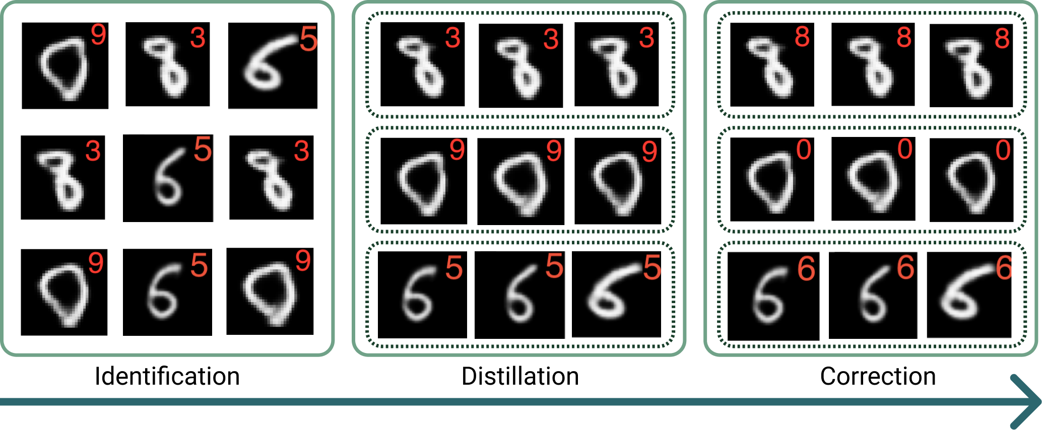
Figure 1: Running Defuse on a MNIST classifier. The (handpicked) images are examples from three misclassification regions identified from running Defuse. The red digit in the upper right hand corner of the image is the classifier’s prediction. Defuse initially identifies many model failures. Next, it aggregates these failures in the distillation step for annotator labeling. Last, Defuse tunes the classifier so that it correctly classifies the images, with minimal change in classifier performance. Defuse serves as an end-to-end framework to diagnose and debug errors in classifiers.

A key goal of machine learning models is generalization. We typically measure generalization through performance on a held-out test set. Ideally, models that score well on held-out test sets should perform the same when deployed. Indeed, researchers track progress using leader boards that use such aggregate statistics [(Russakovsky et al. 2015; Rajpurkar et al. 2016)]. Nevertheless, it has become increasingly apparent test set accuracy alone does not fully describe the performance of machine learning models. For instance, statistics like held out test accuracy may overestimate generalization performance (Recht et al. 2019; Ribeiro et al. 2020; Patel et al. 2008). Also, test statistics offer little insight into or remedy specific model failures (Wu et al. 2019). Last, test data itself is often limited and may not cover all the possible deployment scenarios (Gardner et al. 2020). Because metrics on test set data often fail to describe the performance of machine learning systems fully, it is difficult to verify and trust the behavior of machine learning models when deployed.

As a result, researchers have developed a variety of techniques to evaluate models. Such methods include explanations (Ribeiro, Singh, and Guestrin 2016; Slack et al. 2020; Lundberg and Lee 2017), fairness metrics (Feldman et al. 2015; Ji, Smyth, and Steyvers 2020), and data set replication (Recht et al. 2019; Engstrom et al. 2020). Natural language processing (NLP) has increasingly turned to software engineering inspired behavioral testing tools to find errors in models (Ribeiro et al. 2020). Though these techniques may help find the reasons for misclassifications (e.g., explanations), they do not find novel situations in which the model fails. Other routes to discover model errors are labor-intensive and may require a high amount of task-specific expertise (e.g., dataset replication and behavioral testing). Separately, the adversarial machine learning literature has proposed techniques to generate misclassified inputs for machine learning models automatically. Of particular interest, adversarial machine learning research proposes methods to generate naturally occurring inputs where humans and classifiers disagree called unrestricted or natural adversarial examples (Song et al. 2018; Zhao, Dua, and Singh 2018). Instead of generating imperceptible perturbations like classic adversarial examples, unrestricted adversarial examples find semantically meaningful perturbations that cause models and humans to disagree. The adversarial example literature motivates these instances as a broader security threat than classic adversarial examples (Song et al. 2018). However, techniques that search for unrestricted adversarial examples find diverse instances where classifiers and humans disagree. Thus, unrestricted adversarial examples as a general tool to determine model errors warrant further investigation.

However, several issues arise when using unrestricted adversarial examples in model evaluation setting. For one, unrestricted adversarial examples are generated as single instances and can be found in large quantity even for high-performance classifiers (Song et al. 2018; Zhao, Dua, and Singh 2018). Uncovering actionable and general insights into model errors from a large set of mislabeled instances is highly challenging. Also, human annotators must verify the candidate samples as misclassifications imposing high costs. In this paper, we propose Defuse: a method for debugging classifiers through distilling unrestricted adversarial examples. Defuse facilities using unrestricted adversarial examples to discover and correct model errors while overcoming the issues mentioned earlier. Instead of focusing on single misclassified inputs, the framework provides general insights into model bugs through learning regions in the latent space with many similar errors. We call these regions misclassification regions. Also, Defuse uses the misclassification regions to label many unrestricted adversarial examples more efficiently. All the instances in the region are similar and can receive the same label. Thus, we only need to label the region and not every instance in the region.

For example, we run Defuse on a classifier trained on MNIST and provide an overview in figure 1. Defuse works in three steps: identification, distillation, and correction. In the identification step (first pane in figure 1), Defuse generates unrestricted adversarial examples. The red number in the upper right-hand corner of the image is the classifier’s prediction. Although the classifier achieves high test set performance, we find naturally occurring examples that are classified incorrectly. Next, the method performs the distillation step (second pane in figure 1). The clustering model groups together similar failures for annotator labeling. For instance, Defuse groups together a certain type of incorrectly classified eight in the first row of the second pane in figure 1. Next, Defuse receives annotator labels for each of the clusters. Last, we run the correction step using both the annotator labeled data and the original training data. We see that the model correctly classifies the images (third pane in figure 1). Importantly, the model maintains its predictive performance, scoring $99.1\%$ accuracy after tuning. We see that Defuse serves as a general-purpose method to both discover and correct model errors. We highlight the following contributions of our work:

• We introduce Defuse, a method that can generate many novel model misclassifications through learning misclassification regions in the latent space of a generative model.

• We demonstrate that Defuse finds critical and novel bugs in a number of high performance image classifiers and verify the errors using human evaluation. We also show that Defuse corrects the misclassifications without harming test set generalization.

• We demonstrate the general applicability of unrestricted adversarial examples as a tool for discovering model errors and their usefulness in learning misclassification regions.

2 Notation and Background

In this section, we establish notation and background on unrestricted adversarial examples. Though unrestricted adversarial examples occur in many domains, we focus on Defuse applied to image classification.

Unrestricted adversarial examples

Let $f:\mathbb{R}^{N}\rightarrow[0,1]^{C}$ denote a classifier that accepts a data point $x\in X$, where $X$ is the set of legitimate images. The classifier $f$ returns the probability that $x$ belongs to class $c\in\{1,...,C\}$. Next, assume $f$ is trained on a data set $\mathcal{D}$ consisting of $d$ tuples $(x,y)$ containing data point $x$ and ground truth label $y$ using loss function $\mathcal{L}$. Finally, suppose there exists an oracle $o:x\in X\rightarrow\{1,...,C\}$ that outputs a label for $x$. We define unrestricted adversarial examples as the set $\mathcal{A}_{N}:=\{x\in X\textrm{ }|\textrm{ }o(x)\neq f(x)$} [(Song et al. 2018)].

Variational Autoencoders (VAEs)

In order to find unrestricted adversarial examples, it is necessary to model the set of legitimate images $X$. We use a VAE to create such a model. A VAE is composed of an encoder and a decoder neural networks. These networks are used to model the relationship between data $x$ and latent factors $z\in\mathbb{R}^{K}$. Where $x$ is generated by some ground truth latent factors $v\in\mathbb{R}^{M}$, we wish to train a model such that the learned generative factors closely resemble the true factors: $p(x|v)\approx p(x|z)$. In order to train such a model, we employ the $\beta\textrm{-VAE}$ [(Higgins et al. 2017)]. This technique produces encoder $q_{\phi}(z|x)$ that maps from the data and latent codes and decoder $p_{\theta}(x|z)$ that maps from codes to data.

3 Methods

In this section, we introduce Defuse. We describe the three main steps in the method: identification, distillation, and correction. We also formalize misclassification regions.

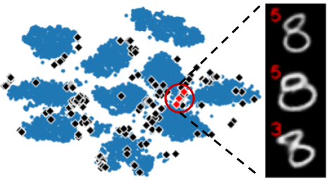
Figure 2: Providing intuition for misclassification regions through a t-SNE visualization of the latent space of MNIST. The black diamonds correspond to the latent codes of unrestricted adversarial examples. The blue circles are the latent codes of images from the training set. The images are three decoded latent codes (the red dots), where the red number in the left-hand corner is the classifier label. We see that there are regions with higher densities of adversarial examples,

3.1 Identification

Algorithm 1 Identification

1:  Identify: $f,p,q,x,y,a,b$

2:  $\psi:=\{\}$

3:  $\mu,\sigma:=q_{\phi}(x)$

4:  for $i\in\{1,...,Q\}$ do

5:     $\epsilon:=[\textrm{Beta}(a,b)_{1},...,\textrm{Beta}(a,b)_{M}]$

6:     $x_{decoded}:=p_{\theta}(\mu+\epsilon)$

7:     if $y\neq f(x_{decoded})$ then

8:        $\psi:=\psi\cup x_{decoded}$

9:     end if

10:  end for

11:  Return $\psi$

This section describes the identification step in Defuse (first pane in figure 1). The aim of the identification step is to generate many unrestricted adversarial examples for a model. We encode all the images from the training data. We perturb the latent codes with a small amount of noise drawn from a Beta distribution. We use a Beta distribution so that it is possible to control the shape of the applied noise. We save instances that are classified differently from ground truth by the model $f$ when decoded. By perturbing the latent codes with a small amount of noise, we expect the decoded instances to have small but semantically meaningful differences from the original instances. Thus, if the classifier prediction deviates from the perturbation, the instance is likely misclassified. We denote the set of unrestricted adversarial examples for a single instance $\psi$. We generate unrestricted adversarial examples over each instance $x\in X$, producing a set of unrestricted adversarial $\Psi$ containing the $\psi$ produced for each instance $x$. We provide pseudocode of the algorithm for generating unrestricted adversarial examples for a single instance $x$ in algorithm 1.

Our technique is related to the method from [(Zhao, Dua, and Singh 2018)]. The authors use a stochastic search method in the latent space of a GAN. They start with a small amount of noise and increase the noise’s magnitude until they find an instance that is predicted differently than the original encoded instance. Because we iterate over the entire data set, it is simpler to keep the noise fixed and sample a predetermined number of times. Critically, we save images that are predicted differently than the ground truth label of the original encoded instance and not just the original prediction. If the model misclassifies the original instance, we wish to save it as a model failure. Otherwise, the method may not find errors associated with inputs that are misclassified incorrectly before perturbation.

3.2 Distillation

We first formalize misclassification regions. Next, we describe the distillation step: our procedure for learning the misclassification regions. Recall, the misclassification regions are regions in the latent space of the generative model with high concentration of unrestricted adversarial examples. The regions provide insight into model bugs and can be used to efficiently correct errors.

Misclassification regions

Let $z\in\mathbb{R}^{K}$ be the latent codes corresponding to image $x\in X$ and $q_{\phi}(\cdot):x\rightarrow z$ be the encoder mapping the relationship between images and latent codes.

Definition 3.1.

Misclassification region. Given a constant $\epsilon>0$, vector norm $||\cdot||$, model $f$, and point $z^{\prime}$, a misclassification regions is a set of images $\mathcal{A}_{R}=\{x\in X\textrm{ }|\textrm{ }\epsilon>||q_{\phi}(x)-z^{\prime}||\land o(x)\neq f(x)\}$.

Previous works that investigate unrestricted adversarial examples look for specific instances where the oracle and the model disagree [(Song et al. 2018; Zhao, Dua, and Singh 2018)]. We instead look for regions in the latent space where this is the case. Because the latent space of the VAE tends to take on Gaussian form due to the prior, we can use euclidean distance to define these regions. If we were to define misclassification regions on the original data manifold, we may need a much more complex distance function. Because it is likely too strict to assume the oracle and model disagree on every instance in such a region, we also introduce a relaxation.

Definition 3.2.

Relaxed misclassification region. Given a constant $\epsilon>0$, vector norm $||\cdot||$, point $z^{\prime}$, model $f$, and threshold $\rho$, a relaxed misclassification regions is a set of images $\mathcal{A}_{f}=\{x\in X\textrm{ }|\textrm{ }\epsilon>||q_{\phi}(x)-z^{\prime}||\}$ such that $|\{x\in\mathcal{A}_{f}\textrm{ }|\textrm{ }o(x)\neq f(x)\}|\textrm{ }/\textrm{ }|\mathcal{A}_{f}|>\rho$.

In this work, we adopt the latter definition of misclassification regions. To concretize misclassification regions and provide evidence for their existence, we continue our MNIST example from figure 1. We plot the t-SNE embeddings of the latent codes of $10000$ images from the training set and $516$ unrestricted adversarial examples created during the identification step in figure 2 (details of how we generate unrestricted adversarial examples in section 3.1). We see that the unrestricted adversarial examples are from similar regions in the latent space.

Distilling misclassification regions

Based on our definition of misclassification regions, we describe a general procedure for learning them. We do so through clustering the latent codes of the unrestricted adversarial examples $\Psi$ in order to diagnose misclassification regions (second pane of figure 1). We require our clustering method to (1) infer the correct number of clusters from the data, and (2) be capable of generating instances of each cluster. We need to infer the number of clusters from the data because the number of misclassification regions is unknown ahead of time. Further, we must generate many instances from each cluster so that we have enough data to finetune on to correct the faulty model behavior. Also, generating many failure instances enables model designers to see numerous examples from the misclassification regions, which encourages understanding the model failure modes. Though any such clustering method under this description is compatible with distillation, we use a Gaussian mixture model (GMM) with the Dirichlet process prior. We use the Dirichlet process because it describes the clustering problem where the number of mixtures is unknown beforehand, fulfilling our first criteria [(Sudderth 2006)]. Additionally, because the model is generative, we can sample new instances, satisfying our second criteria.

In practice, we use the truncated stick-breaking construction of the Dirichlet process, where $K$ is the upper bound of the number of mixtures. The truncated stick-breaking construction simplifies inference making computation more efficient [(Sudderth 2006)]. The method outputs a set of clusters $\theta_{j}=(\mu_{j},\sigma_{j},\pi_{j})$ where $j\in\{1,...,K\}$. The parameters $\mu$ and $\sigma$ describe the mean and variance of a multivariate normal distribution and $\pi$ indicates the cluster weight. To perform inference on the model, we employ expectation maximization (EM) described in [(Bishop 2006)] and use the implementation provided in [(Pedregosa et al. 2011)]. Once we run EM and determine the parameter values, we throw away cluster components that are not used by the model. We fix some small $\epsilon$ and define the set of misclassification regions $\Lambda$ generated at the distillation step as: $\Lambda:=\{(\mu_{j},\Sigma_{j},\pi_{j})|\pi_{j}>\epsilon\}$.

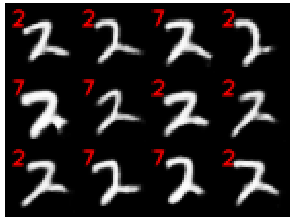
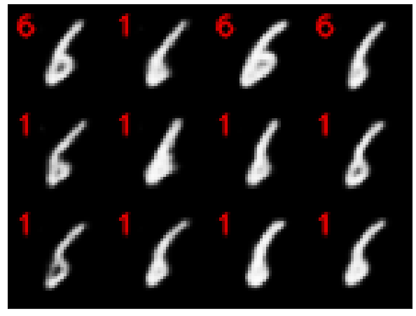
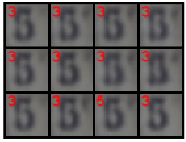
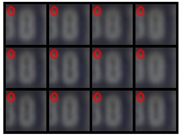
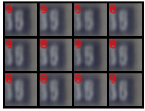
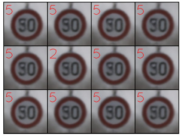
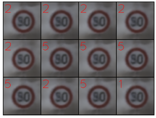
Figure 3: Samples from three misclassification regions from each dataset. First row: The MNIST misclassification regions. These scenarios were labeled $4$, $2$, $6$ in order from left to right. Second row: The SVHN misclassification regions labeled $5$, $8$, and $5$ from left to right. Third row: The German signs misclassification regions. The label $1$ corresponds to $30$km/h, $2$ to $50$km/h, and $5$ to $80$km/h. The first and second were labeled $2$ while the third was labeled $1$. Defuse finds significant bugs in the classifiers.

3.3 Correction

This section describes the procedure for labeling the misclassification regions and finetuning the model to fix the classifier errors.

Labeling

First, an annotator assigns the correct label to the misclassification regions. For each misclassification regions identified in $\Lambda$, we sample $Q$ latent codes from $z\sim\mathcal{N}(\mu_{j},\tau\cdot\sigma_{j})$. Here, $\tau\in\mathbb{R}$ is a hyperparameter that controls sample diversity from the misclassification regions. Because it could be possible for multiple ground truth classes to be present in a misclassification region, we set this parameter tight enough such that the sampled instances are from the same class. We reconstruct the latent codes using the decoder $p_{\theta}(x|z)$. Next, an annotator reviews the reconstructed instances from the scenario and decides whether the scenario constitutes a model failure. If so, the annotator assigns the correct label to all of the instances. The correct label constitutes a single label for all of the instances generated from the scenario. We repeat this process for each of the scenarios identified in $\Lambda$ and produce a dataset of failure instances $\mathcal{D}_{f}$. Pseudocode for the procedure is given in algorithm 3 in appendix A.

Finetuning

We finetune on the training data with an additional regularization term to fix the classifier performance on the misclassification regions. The regularization term is the cross-entropy loss between the identified misclassification regions and the annotator label. Where $\mathcal{L}$ is the cross-entropy loss applied to the failure instances $\mathcal{D}_{f}$ and $\lambda$ is the hyperparameter for the regularization term, we optimize the following objective using gradient descent,

$$\mathcal{F}(\mathcal{D},\mathcal{D}_{f})=\mathcal{L}(\mathcal{D})+\lambda\cdot\mathcal{L}(\mathcal{D}_{f})$$ (1)

This objective encourages the model to maintain its predictive performance on the original training data while encouraging the model to predict the failure instances correctly. The regularization term $\lambda$ controls the pressure applied to the model to classify the failure instances correctly.

4 Experiments

	Dataset	# Scenarios	Validation	Test	Misclassification Region
Before Finetuning	MNIST	-	-	98.3	29.1
	SVHN	-	93.6	93.2	31.2
	German Signs	-	98.8	98.7	27.8
Unrestricted	MNIST	-	-	99.1	58.3
Adversarial Examples	SVHN	-	93.1	92.9	65.4
	German Signs	-	-	-	-
Defuse	MNIST	19	-	99.1	96.4
	SVHN	6	93.0	92.8	99.9
	German Signs	8	98.1	97.7	85.6

Figure 4: Results from the best models before finetuning, finetuning only on the unrestricted adversarial examples, and finetuning using Defuse. The numbers presented are accuracy on the validation, test set, and misclassification region test set and the absolute number of misclassification regions generated using Defuse. We do not include finetuning on the unrestricted adversarial examples for German Signs because we, the authors, assigned misclassification regions for this data set and thus do not have ground truth labels for individual examples. Critically, the test accuracy on the misclassification regions is high for Defuse indicating that the method successfully corrects the faulty behavior.

4.1 Setup

Datasets We evaluate Defuse on three datasets: MNIST [(LeCun, Cortes, and Burges 2010)], the German Traffic Signs dataset [(Stallkamp et al. 2011)], and the Street view house numbers dataset (SVHN) [(Netzer et al. 2011)]. MNIST consists of $60,000$ $32\textrm{X}32$ handwritten digits for training and $10,000$ digits for testing. The images are labeled corresponding to the digits $0-9$. The German traffic signs data set includes $26,640$ training and $12,630$ testing images of size $128\textrm{X}128$. We randomly split the testing data in half to produce a validation and testing set. The images are labeled from $43$ different classes to indicate the type of traffic signs. The SVHN data set consists of $73,257$ training and $26,032$ testing images of size $32\textrm{X}32$. The images include digits of house numbers from Google streetview with labels $0-9$. We split the testing set in half to produce a validation and testing set.

Models On MNIST, we train a CNN scoring $98.3\%$ test set accuracy following the architecture from [(Paszke et al. 2019)]. On German traffic signs and SVHN, we finetune a Resnet18 model pretrained on ImageNet [(He et al. 2016)]. The German signs and SVHM models score $98.7\%$ and $93.2\%$ test accuracy respectively. We train a $\beta$-VAE the on the training data set to model the set of legitimate images in Defuse. We use an Amazon EC2 P3 instance with a single NVIDIA Tesla V100 GPU for training. We follow similar architectures to [(Higgins et al. 2017)]. We set the size of the latent dimension $z$ to $10$ for MNIST/SVHN and $15$ for German signs. We provide our $\beta$-VAE architectures in appendix B.

Defuse We run Defuse on each classifier. In the identification step, we fix the parameters of the Beta distribution noise $a$ and $b$ to $a=b=50.0$ for MNIST and $a=b=75.0$ for SVHN and German signs. We found these parameters were good choices because they produce a minimal amount of perturbation noise, making the decoded instances slightly different from the original instances. During distillation, we set the upper bound on the number of components $K$ to $100$. We generally found the actual number of clusters to be much lower than this level. Thus, this serves as an appropriate upper bound. We also fixed the weight threshold for clusters $\epsilon$ to $0.01$ during distillation to remove clusters with very low weighting. We also randomly downsample the number of unrestricted adversarial examples to $50,000$ to make the GMM more efficient. We sample finetuning and testing sets consisting of $256$ images each from every misclassification region for correction. We found empirically that this number of samples is appropriate because it captures the breadth of possible images in the scenario. We use the finetuning set as the set of failure instances $\mathcal{D}_{f}$. We used the test set as held out data to evaluate classifier performance on the misclassification regions after correction. During sampling, we fix the sample diversity $\tau$ to $0.5$ for MNIST and $0.01$ for SVHN and German signs because the samples from each of the misclassification regions appear to be in the same class using these values. During correction, we finetune over a range of $\lambda$’s to find the best balance between training and misclassification region data. We use $3$ epochs for MNIST and $5$ for both SVHN and German Signs because training converged within this amount of epochs. During finetuning, we select the model for each $\lambda$ according to the highest training set accuracy for MNIST or validation set accuracy for SVHM and German traffic signs at the end of each finetuning epoch. We select the best model overall as the highest training or validation performance over all $\lambda$’s.

Annotator Labeling Because Defuse requires human supervision, we use Amazon Sagemaker Ground Truth human workers to both determine whether clusters generated in the distillation step are misclassification regions and to generate their correct label. To determine whether clusters are misclassification regions, we sample $10$ instances from each cluster in the distillation step. It is usually apparent the classifier disagrees with many of the ground truth labels within $10$ instances, and thus it is appropriate to label the cluster as a misclassification region. To reduce noise in the annotation process, we assign the same image to $5$ different workers and take the majority annotated label as ground truth. The workers label the images using an interface that includes a single image and the possible labels for that task. We additionally instruct workers to select “None of the above” if the image does not belong to any class and discard these labels. For instance, the MNIST interface includes a single image and buttons for the digits $0-9$ along with a “None of the above” button. We provide a screenshot of this interface in figure 15. If more than half (i.e. setting $\rho=0.5$) of worker labeled instances disagree with the classifier predictions on the $10$ instances, we call the cluster a misclassification region. We chose $\rho=0.5$ because clusters are highly dense with incorrect predictions at this level, making them useful for both understanding model failures and worthwhile for correction. We take the majority prediction over each of the $10$ ground truth labels as the label for the misclassification region. As an exception, annotating the German traffic signs data requires specific knowledge of traffic signs. The German traffic signs data ranges across $43$ different types of traffic signs. It is not reasonable to assume annotators have enough familiarity with this data and can label it accurately. For this data set, we, the authors, reviewed the distilled clusters and determined which clusters constituted misclassification regions. We labeled the clusters with more than half of the instances misclassified as misclassification regions. Though this procedure is less rigorous, the results still provide good insight into the model bugs discovered by Defuse.

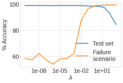
(a) MNIST

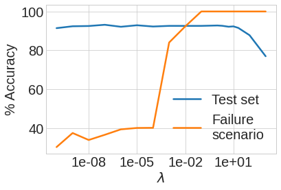
(b) SVHN

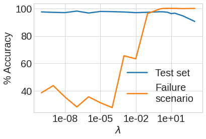
(c) German Signs

Figure 5: The tradeoff between test set and misclassification region accuracy running correction. We assess both test set accuracy and accuracy on the test misclassification region data finetuning over a range of $\lambda$’s and plot the trade off. There is an optimal $\lambda$ for each classifier where test set and misclassification region accuracy are both high. This result confirms that the correction step in Defuse adequately balances both generalization and accuracy on the misclassification regions .

4.2 Illustrative misclassification region examples

We demonstrate Defuse’s potential to identify critical model bugs. We review misclassification regions from three datasets we consider. Defuse returns $19$ misclassification regions for MNIST, $6$ for SVHN, and $8$ for German signs. We provide samples from three misclassification regions for each dataset in figure 3. The misclassification regions include numerous mislabeled examples of similar style. For example, in MNIST, the misclassification region in the upper left-hand corner of figure 3 includes a similar style of incorrectly predicted $4$’s. The misclassification regions generally include “corner case” images. These images are challenging to classify and thus highly insightful from a debugging perspective. For instance, the misclassified $6$’s are relatively thin, making them appear like $1$’s in some cases. There are similar trends in SVHN and German Signs. In SVHN, the model misclassifies particular types of $5$’s and $8$’s. The same is true in German signs, where the model predicts styles of $50$km/h and $30$km/h signs incorrectly. We provide additional samples from other misclassification regions in appendix D. These results demonstrate Defuse uncovers significant and insightful model bugs.

4.3 Novely of the errors

We expect Defuse to find novel model misclassifications beyond those revealed by the available data. Thus, it is critical to evaluate whether the errors produced by Defuse are the same as those already in the training data. We compare the similarity of the errors proposed by Defuse (the misclassification region data) and the misclassified training data. We perform this analysis on MNIST. We choose $10$ images from the misclassification regions and find the nearest neighbor in the misclassified training data according to $\ell_{2}$ distance. We provide the results in figure 6. We see that the data in the misclassification regions reveal different types of errors than the training set.

Interestingly, though some of the images are quite similar, they are predicted differently by the model. This result indicates the misclassification regions reveal new model failures. These results demonstrate Defuse can be used to reveal novel sources of model error.

Misclassified Training Set
Misclassification Region

Figure 6: Assessing the novelty of errors in misclassification regions. We compare samples from the misclassification regions with the nearest neighbors in the misclassified training set data. We see that the misclassification regions reveal novel sources of model error not found in the misclassified training data.

4.4 Correcting misclassification regions

After running correction, classifier accuracy should improve on the misclassification region data indicating we have corrected the bugs discovered in earlier steps. Also, the classifier accuracy on the test set should stay at a similar level or improve, indicating that the model generalization according to the test set is still strong. We show that this is the case using Defuse. We assess accuracy on both the misclassification region test data and the original test set after performing correction. We compare Defuse against finetuning only on the unrestricted adversarial examples labeled by annotators. We expect this baseline to be reasonable because related works that focus on robustness to classic adversarial attacks demonstrate the effectiveness of tuning directly on the adversarial examples [(Zhang et al. 2019)]. We finetune on the unrestricted adversarial examples sweeping over a range of different $\lambda$’s and taking the best model as described in section 4.1. We use this baseline for MNIST and SVHN but not German Signs because we do not have ground truth labels for unrestricted adversarial examples.

We provide an overview of the models before finetuning, finetuning with the unrestricted adversarial examples, and using Defuse in figure 4. Defuse scores highly on the misclassification region data after correction compared to before finetuning. There is only a marginal improvement in the baseline. These results indicate Defuse corrects the faulty model performance on the misclassification regions. Also, these results show the clustering step in Defuse is critical to its success. We see this because finetuning on the unrestricted adversarial examples performs worse than finetuning on the misclassification regions. Last, there are minor effects on test set performance during finetuning, demonstrating Defuse does not harm generalization according to the test set.

Further, we plot the relationship between test set accuracy and misclassification region test accuracy in figure 5 varying over $\lambda$. There is an appropriate $\lambda$ for each model where test set accuracy and accuracy on the misclassification regions are both high. Overall, these results indicate the correction step in Defuse is highly effective at correcting the errors discovered during identification and distillation.

4.5 Annotator Agreement

Because we rely on annotators to provide the ground truth labels for the unrestricted adversarial examples, we investigate the agreement between the annotators during labeling. The annotators should agree on the labels for the unrestricted adversarial examples. Agreement indicates we have high confidence our evaluation is based on accurately labeled data. We evaluate the annotator agreement by assessing the percent of annotators that voted for the majority label prediction for a single instance. This metric will be high when the annotators agree and low when only a few annotators constitute the majority vote. Further, we calculate the annotator agreement for every annotated instance. We provide the annotator agreement on MNIST and SVHN in figure 7 broken down into misclassification region data, non-misclassification region data, and their combination.

Interestingly, the misclassification region data has slightly lower annotator agreement indicating these tend to be more ambiguous examples. Further, there is lower agreement on SVHN than MNIST, likely because this data is more complex. All in all, there is generally high annotator agreement across all the data.

Dataset	M.R.	Non-M.R.	Combined
MNIST	$78.9.3\pm 5.4$	$87.2\pm 3.2$	$85.2\pm 0.1$
SVHN	$66.6\pm 8.4$	$83.2\pm 4.1$	$82.1\pm 1.3$

Figure 7: Annotator agreement on the unrestricted adversarial examples. We plot the mean and standard error of the percent of annotators that voted for the majority label in an unresricted adversarial example across all the annotated examples. We break this down into the misclassification region (M.R.) and non-misclassification region (Non-M.R.) unrestricted adversarial examples and the combination between the two. The annotators are generally in agreement though less so for the misclassification region data, indicating these tend to be more ambiguous examples.

5 Related Work

A number of related approaches for improving classifier performance use data created from generative models — mostly generative adversarial networks (GANs) [(Sandfort et al. 2019; Milz, Rudiger, and Suss 2018; Antoniou, Storkey, and Edwards 2017)]. These methods use GANs to generate instances from classes that are underrepresented in the training data to improve generalization performance. Additional methods use generative models for semi-supervised learning [(Kingma et al. 2014; Varma et al. 2016; Kumar, Sattigeri, and Fletcher 2017; Dumoulin et al. 2016)]. Though these methods are similar in nature to the correction step of our work, a key difference is Defuse focuses on summarizing and presenting high level model failures. Also, [(Varma et al. 2017)] provide a system to debug data generated from a GAN when the training set may be inaccurate. Though similar, we ultimately use a generative model to debug a classifier and do not focus on the generative model itself. Last, similar to [(Song et al. 2018), (Zhao, Dua, and Singh 2018)], [(Booth et al. 2021)] provide a method to generate highly confident misclassified instances.

One aspect of our work looks at improving performance on unrestricted adversarial examples. Thus, there are similarities between our work and methods that improve robustness to adversarial attacks. Similar to Defuse, several techniques demonstrate that tuning on additional data helps improve classic adversarial robustness. (Carmon et al. 2019) demonstrate robustness is improved with the addition of unlabeled data during training. Also, (Zhang, Zhu, and Wright 2018) show directly training on the adversarial examples improves robustness. (Raghunathan et al. 2020) characterize a trade-off between robustness and accuracy in perturbation based data augmentations during adversarial training. Because we train with on manifold data created by generative models, there is not so much of a trade-off between robustness and accuracy. We find that we can achieve high performance on the unrestricted adversarial examples with minimal change to test accuracy. Though related, our work demonstrates that robustness to naturally occurring adversarial examples show different robustness dynamics than classic adversarial examples.

Related to debugging models, [(Kang et al. 2018)] focus on model assertions that flag failures during production. Also, [(Zhang, Zhu, and Wright 2018)] investigate debugging the training set for incorrectly labeled instances. We focus on preemptively identifying model bugs and do not focus on incorrectly labeled test set instances. Additionally, [(Ribeiro et al. 2020)] propose a set of behavioral testing tools that help model designers find bugs in NLP models. This technique requires a high level of supervision and thus might not be appropraite in some settings. Last, [(Odena et al. 2019)] provide a technique to debug neural networks through perturbing data inputs with various types of noise. By leveraging unrestricted adversarial examples, we distill high level patterns in critical and naturally occurring model bugs. This technique requires minimal human supervision while presenting important types of model errors to designers.

6 Conclusion

In this paper, we present Defuse: a method that generates and aggregates unrestricted adversarial examples to debug classifiers. Though previous works discuss unrestricted adversarial examples, we harness such examples to debug classifiers. We accomplish this task by identifying misclassification regions: regions in the latent space of a VAE with many unrestricted adversarial examples. On various data sets, we find that samples from misclassification regions are useful in many ways. First, misclassification regions are informative for understanding the ways specific models fail. Second, the generative aspect of misclassification regions is beneficial for correcting misclassification regions. Our experimental results show that these misclassification regions include critical model issues for classifiers with real world impacts (i.e. traffic sign classification) and verify our results using ground truth annotator labels. We demonstrate that Defuse successfully resolves these issues. A potential direction for future research is to explore directly optimizing for the misclassification regions instead of using unrestricted adversarial examples. Another direction worth exploring is to evaluate the success of Defuse applied to large, state of the art generative models.

Appendix A Defuse Psuedo Code

In algorithm 3, $\texttt{Correct}(\cdot)$ and $\texttt{Label}(\cdot)$ are the steps where the annotator decides if the scenario warrants correction and the annotator label for the misclassification region.

Algorithm 2 Identification

1:  Identify: $f,p,q,x,y,a,b$

2:  $\psi:=\{\}$

3:  $\mu,\sigma:=q_{\phi}(x)$

4:  for $i\in\{1,...,Q\}$ do

5:     $\epsilon:=[\textrm{Beta}(a,b)_{1},$

6:             $...,\textrm{Beta}(a,b)_{M}]$

7:     $x_{decoded}:=p_{\theta}(\mu+\epsilon)$

8:     if $y\neq f(x_{decoded})$ then

9:        $\psi:=\psi\cup x_{decoded}$

10:     end if

11:  end for

12:  Return $\psi$

Algorithm 3 Labeling

  Label Scenarios $Q,\Lambda,p,q,\tau$

  $D_{f}:=\{\}$

  for $(\mu,\sigma,\pi)\in\Lambda$ do

     $X_{d}:=\{\}$

     for $i\in\{1,..,Q\}$ do

        $X_{d}:=X_{d}\cup q_{\psi}(\mathcal{N}(\mu,\tau\cdot\sigma))$

     end for

     if Correct$(X_{d})$ then

        $D_{f}:=D_{f}\cup\{X_{d},\textrm{{Label}}(X_{d})\}$

     end if

  end for

  Return $\bigcup D_{f}$

Appendix B Training details

B.1 GMM details

In all experiments, we use the implementation of Gaussian mixture model with dirichlet process prior from [(Pedregosa et al. 2011)]. We run our experiments with the default parameters and full component covariance.

B.2 MNIST details

Model details

We train a CNN on the MNIST data set using the architecture in figure 8. We used the Adadelta optimizer with the learning rate set to $1$. We trained for $5$ epochs with a batch size of $64$.

Architecture
4x4 conv., 64 ReLU stride 2
4x4 conv., 64 ReLU stride 2
4x4 conv., 64 ReLU stride 2
4x4 conv., 64 ReLU stride 2
Fully connected 256, ReLU
Fully connected 256, ReLU
Fully connected 10 $\times$ 2

Figure 8: MNIST CNN Architecture

$\beta$-VAE training details

We train a $\beta$-VAE on MNIST using the architectures in figure 9 and 10. We set $\beta$ to $4$. We trained for $800$ epochs using the Adam optimizer with a learning rate of $0.001$, a minibatch size of $2048$, and $\beta$ set to $0.4$. We also applied a linear annealing schedule on the KL-Divergence for $500$ optimization steps. We set $z$ to have $10$ dimensions.

Architecture
4x4 conv., 32 ReLU stride 2
4x4 conv., 32 ReLU stride 2
4x4 conv., 32 ReLU stride 2
Fully connected 256, ReLU
Fully connected 256, ReLU
Fully connected 15 $\times$ 2

Figure 9: MNIST data set encoder architecture.

Architecture
Fully connected 256, ReLU
Fully connected 256, ReLU
Fully connected 256, ReLU
4x4 transpose conv., 32 ReLU stride 2
4x4 transpose conv., 32 ReLU stride 2
4x4 transpose conv., 32 ReLU stride 2
4x4 transpose conv., 32 Sigmoid stride 2

Figure 10: MNIST data set decoder architecture.

Identification

We performed identification with $Q$ set to $500$. We set $a$ and $b$ both to $50$. We ran identification over the entire training set. Last, we limited the max allowable size of $\psi$ to $100$.

Distillation

We ran the distillation step setting $K$, the upper bound on the number of mixtures, to $100$. We fixed $\epsilon$ to $0.01$ and discarded clusters with mixing proportions less than this value. This left $44$ possible scenarios. We set $\tau$ to $0.5$ during review. We used Amazon Sagemaker Ground Truth to determine misclassification regions and labels. The labeling procedure is described in section 4.1. This produced $19$ misclassification regions.

Correction

We sampled $256$ images from each of the misclassification regions for both finetuning and testing. We finetuned with minibatch size of $256$, the Adam optimizer, and learning rate set to $0.001$. We swept over a range of correction regularization $\lambda$’s consisting of $[1e-10,1e-9,1e-8,1e-7,1e-6,1e-5,1e-4,1e-3,1e-2,1e-1,1,2,5,10,20,100,1000]$ and finetuned for $3$ epochs on each.

B.3 German Signs Dataset Details

Dataset

The data consists of $26640$ training images and $12630$ testing images consisting of 43 different types of traffic signs. We randomly split the testing data in half to produce $6315$ testing and validation images. Additionally, we resize the images to $128\textrm{x}128$ pixels.

Classifier $f$

We fine-tuned the ResNet18 model for $20$ epochs using Adam with the cross entropy loss, learning rate of $0.001$, batch size of $256$ on the training data set, and assessed the validation accuracy at the end of each epoch. We saved the model with the highest validation accuracy.

$\beta$-VAE training details

We trained for $800$ epochs using the Adam optimizer with a learning rate of $0.001$, a minibatch size of $2048$, and $\beta$ set to $4$. We also applied a linear annealing schedule on the KL-Divergence for $500$ optimization steps. We set $z$ to have $15$ dimensions.

Architecture
4x4 conv., 64 ReLU stride 2
4x4 conv., 64 ReLU stride 2
4x4 conv., 64 ReLU stride 2
4x4 conv., 64 ReLU stride 2
Fully connected 256, ReLU
Fully connected 256, ReLU
Fully connected 15 $\times$ 2

Figure 11: German signs data set encoder architecture.

Architecture
Fully connected 256, ReLU
Fully connected 256, ReLU
Fully connected 256, ReLU
4x4 transpose conv., 64 ReLU stride 2
4x4 transpose conv., 64 ReLU stride 2
4x4 transpose conv., 64 ReLU stride 2
4x4 transpose conv., 64 ReLU stride 2
4x4 transpose conv., 64 Sigmoid stride 2

Figure 12: German signs data set decoder architecture.

Identification

We performed identification with $Q$ set to $100$. We set $a$ and $b$ both to $75$.

Distillation

We ran the distillation step setting $K$ to $100$. We fixed $\epsilon$ to $0.01$ and discarded clusters with mixing proportions less than this value. This left $38$ possible scenarios. We set $\tau$ to $0.01$ during review. We determined $8$ of these scenarios were particularly concerning.

Correction

We finetuned with minibatch size of $256$, the Adam optimizer, and learning rate set to $0.001$. We swept over a range of correction regularization $\lambda$’s consisting of $[1e-10,1e-9,1e-8,1e-7,1e-6,1e-5,1e-4,1e-3,1e-2,1e-1,1,2,5,10,20,100,1000]$ and finetuned for $5$ epochs on each.

B.4 SVHN details

Dataset

The data set consists of $73257$ training and $26032$ testing images. We also randomly split the testing data to create a validation data set. Thus, the final validation and testing set correspond to $13016$ images each.

Classifier $f$

We fine tuned for $10$ epochs using the Adam optimizer, learning rate set to $0.001$, and a batch size of $2048$. We chose the model which scored the best validation accuracy when measured at the end of each epoch.

$\beta$-VAE training details

We trained the $\beta$-VAE for $400$ epochs using the Adam optimizer, learning rate $0.001$, and minibatch size of $2048$. We set $\beta$ to $4$ and applied a linear annealing schedule on the Kl-Divergence for $5000$ optimization steps. We set $z$ to have $10$ dimensions.

Architecture
4x4 conv., 64 ReLU stride 2
4x4 conv., 64 ReLU stride 2
4x4 conv., 64 ReLU stride 2
Fully connected 256, ReLU
Fully connected 256, ReLU
Fully connected 10 $\times$ 2

Figure 13: SVHN data set encoder architecture.

Architecture
Fully connected 256, ReLU
Fully connected 256, ReLU
Fully connected 256, ReLU
4x4 transpose conv., 64 ReLU stride 2
4x4 transpose conv., 64 ReLU stride 2
4x4 transpose conv., 64 ReLU stride 2
4x4 transpose conv., 64 Sigmoid stride 2

Figure 14: SVHN data set decoder architecture.

Identification

We set $Q$ to $100$. We also set the maximum size of $\psi$ to $10$. We set $a$ and $b$ to $75$.

Distillation

We set $K$ to $100$. We fixed $\epsilon$ to $0.01$. The distillation step identified $32$ plausible misclassification regions. The annotators deemed $6$ of these to be misclassification regions. We set $\tau$ to $0.01$ during review.

Correction

We set the minibatch size of $2048$, the Adam optimizer, and learning rate set to $0.001$. We considered a range of $\lambda$’s: $[1e-10,1e-9,1e-8,1e-7,1e-6,1e-5,1e-4,1e-3,1e-2,1e-1,1,2,5,10,20,100,1000]$. We finetuned for $5$ epochs.

B.5 t-SNE example details

We run t-SNE on $10,000$ examples from the training data and $516$ unrestricted adversarial examples setting perplexity to $30$. For the sake of clarity, we do not include outliers from the unrestricted adversarial examples. Namely, we only include unrestricted adversarial examples with $>1\%$ probabilitdefuse-iclr clusters.

Appendix C Annotator interface

We provide a screenshot of the annotator interface in figure 15.

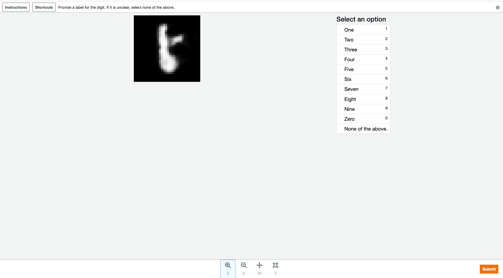
Figure 15: Annotation interface.

Appendix D Additional experimental results

D.1 Additional samples from MNIST misclassification regions

We provide additional examples from $10$ randomly selected (no cherry picking) MNIST misclassification regions. We include the annotator consensus label for each misclassification region.

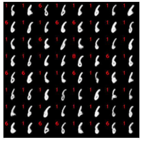
Figure 16: Annotator label $6$.

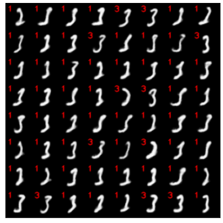
Figure 17: Annotator label $3$.

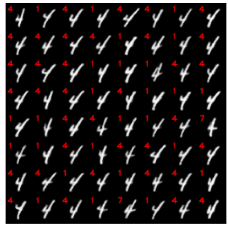
Figure 18: Annotator label $4$.

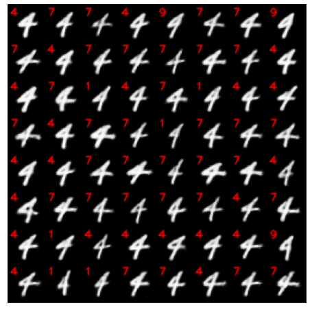
Figure 19: Annotator label $4$.

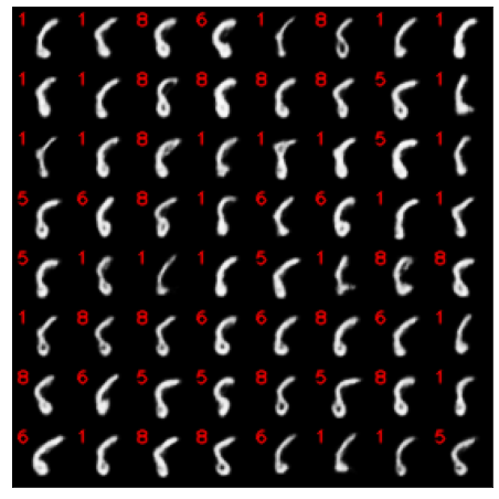
Figure 20: Annotator label $6$.

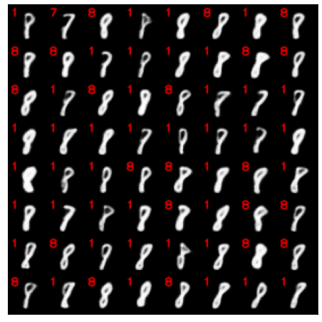
Figure 21: Annotator label $8$.

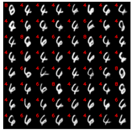
Figure 22: Annotator label $6$.

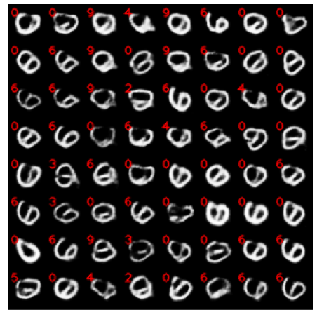
Figure 23: Annotator label $0$.

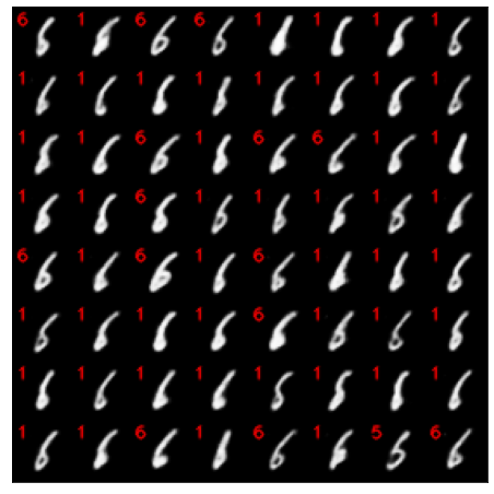
Figure 24: Annotator label $6$.

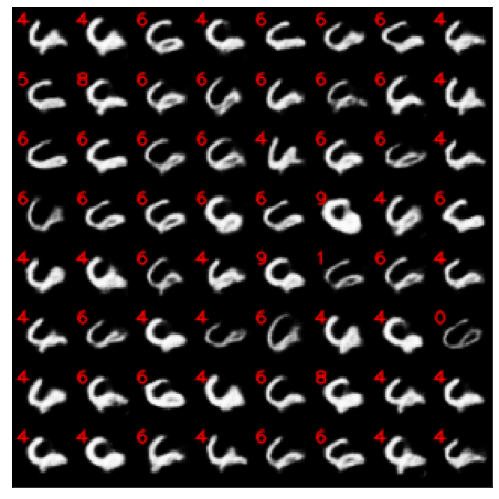
Figure 25: Annotator label $6$.

D.2 Additional samples from German signs misclassification regions

We provide samples from all of the German signs misclassification regions. We provide the names of the class labels in figure 26. For each misclassification region, we indicate our assigned class label in the caption and the classifier predictions in the upper right hand corner of the image.

ClassId	SignName
0	Speed limit (20km/h)
1	Speed limit (30km/h)
2	Speed limit (50km/h)
3	Speed limit (60km/h)
4	Speed limit (70km/h)
5	Speed limit (80km/h)
6	End of speed limit (80km/h)
7	Speed limit (100km/h)
8	Speed limit (120km/h)
9	No passing
10	No passing for vehicles over 3.5 metric tons
11	Right-of-way at the next intersection
12	Priority road
13	Yield
14	Stop
15	No vehicles
16	Vehicles over 3.5 metric tons prohibited
17	No entry
18	General caution
19	Dangerous curve to the left
20	Dangerous curve to the right
21	Double curve
22	Bumpy road
23	Slippery road
24	Road narrows on the right
25	Road work
26	Traffic signals
27	Pedestrians
28	Children crossing
29	Bicycles crossing
30	Beware of ice/snow
31	Wild animals crossing
32	End of all speed and passing limits
33	Turn right ahead
34	Turn left ahead
35	Ahead only
36	Go straight or right
37	Go straight or left
38	Keep right
39	Keep left
40	Roundabout mandatory
41	End of no passing
42	End of no passing by vehicles over 3.5 metric tons

Figure 26: German signs class labels.

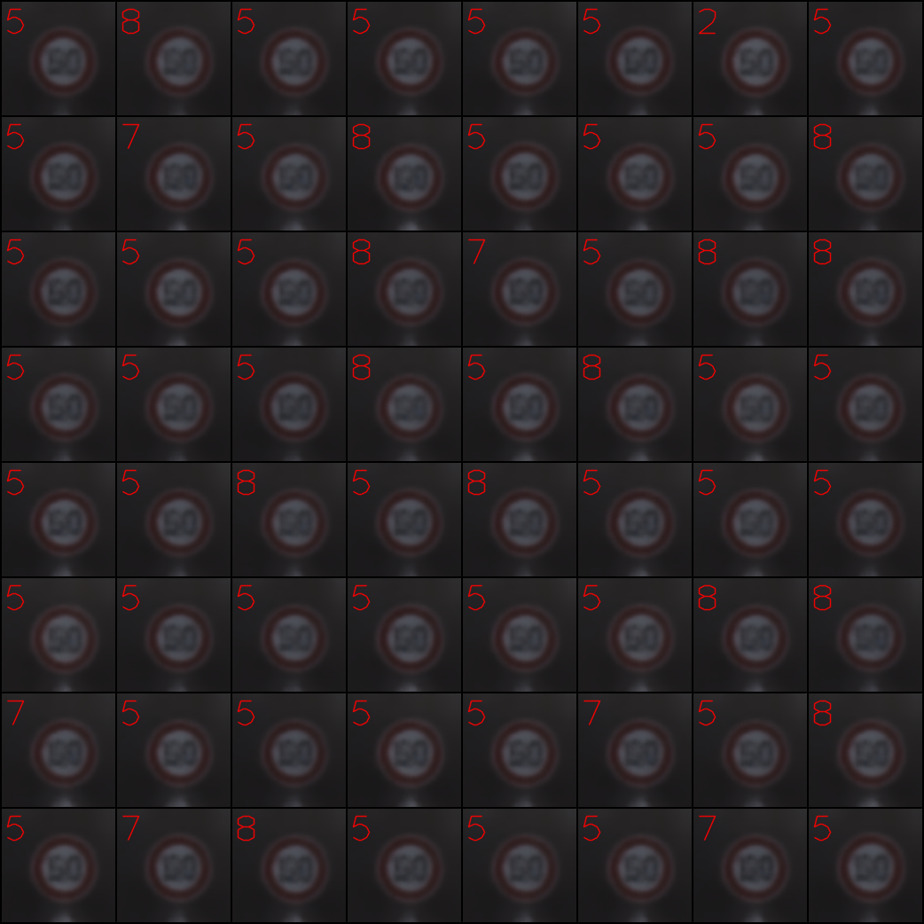
Figure 27: Annotator label $7$.

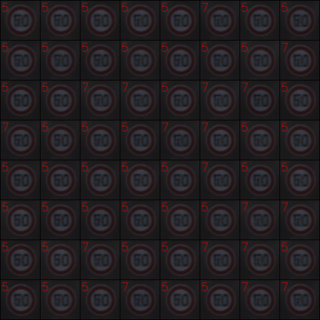
Figure 28: Annotator label $2$.

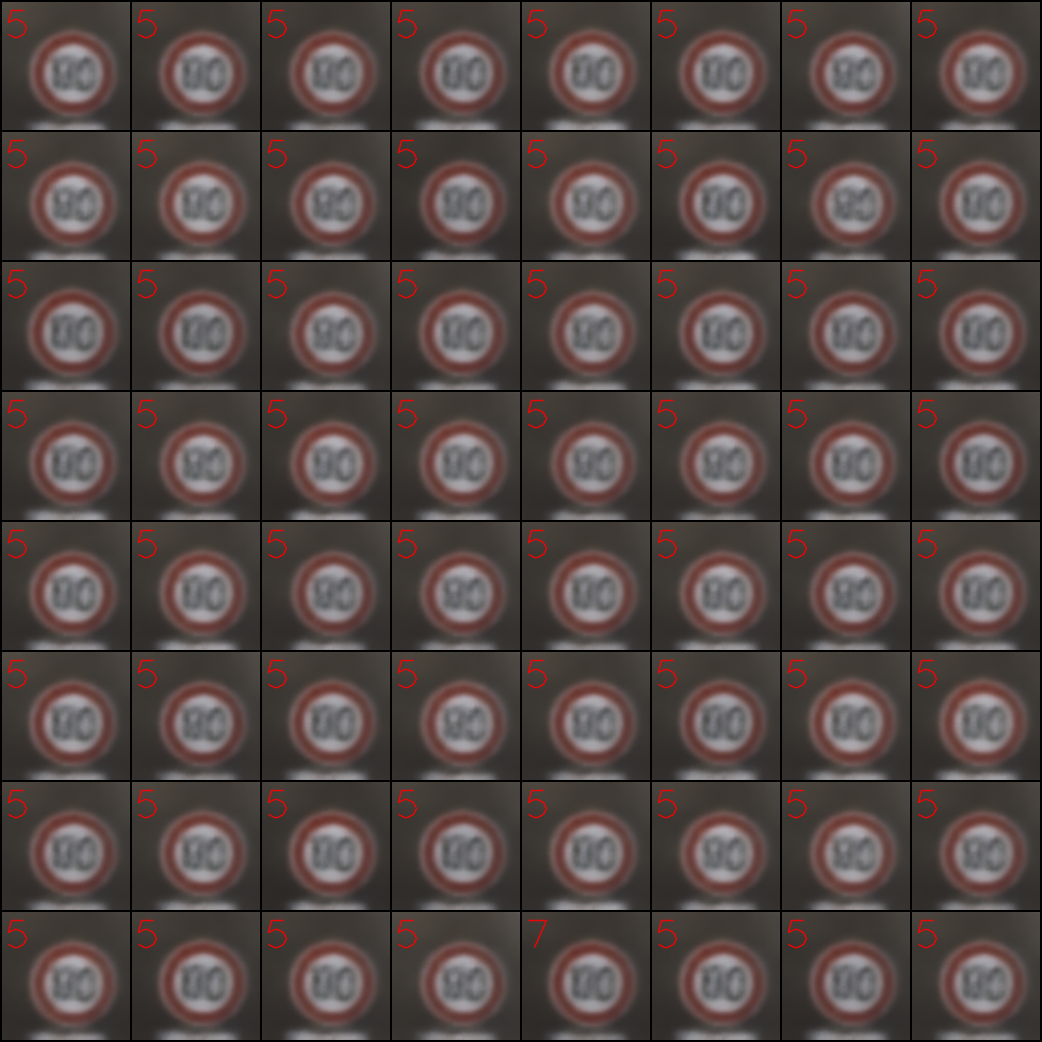
Figure 29: Annotator label $7$.

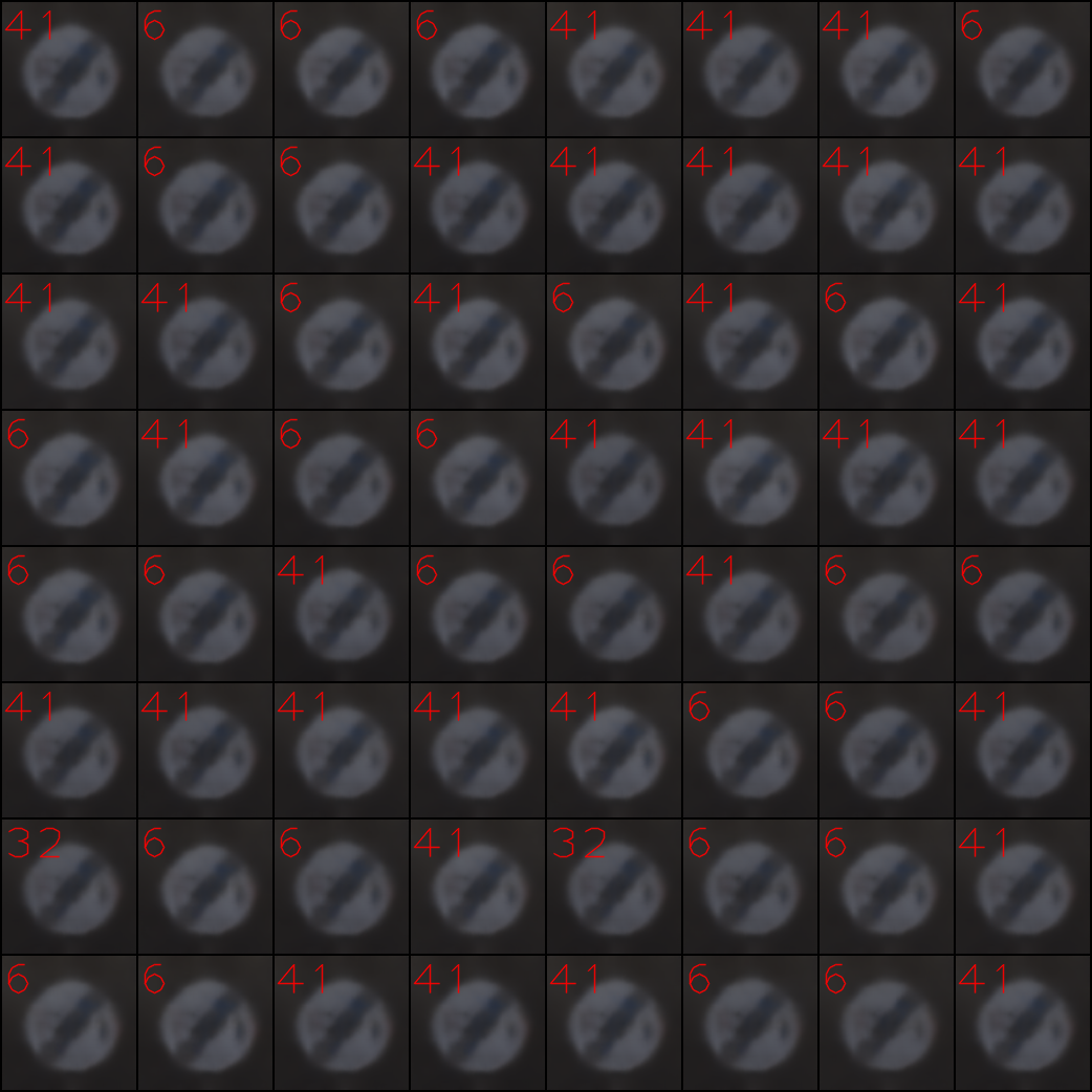
Figure 30: Annotator label $41$.

Figure 31: Annotator label $1$.

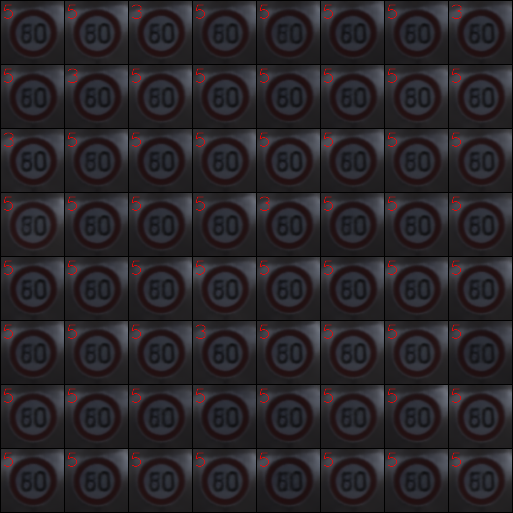
Figure 32: Annotator label $2$.

Figure 33: Annotator label $2$.

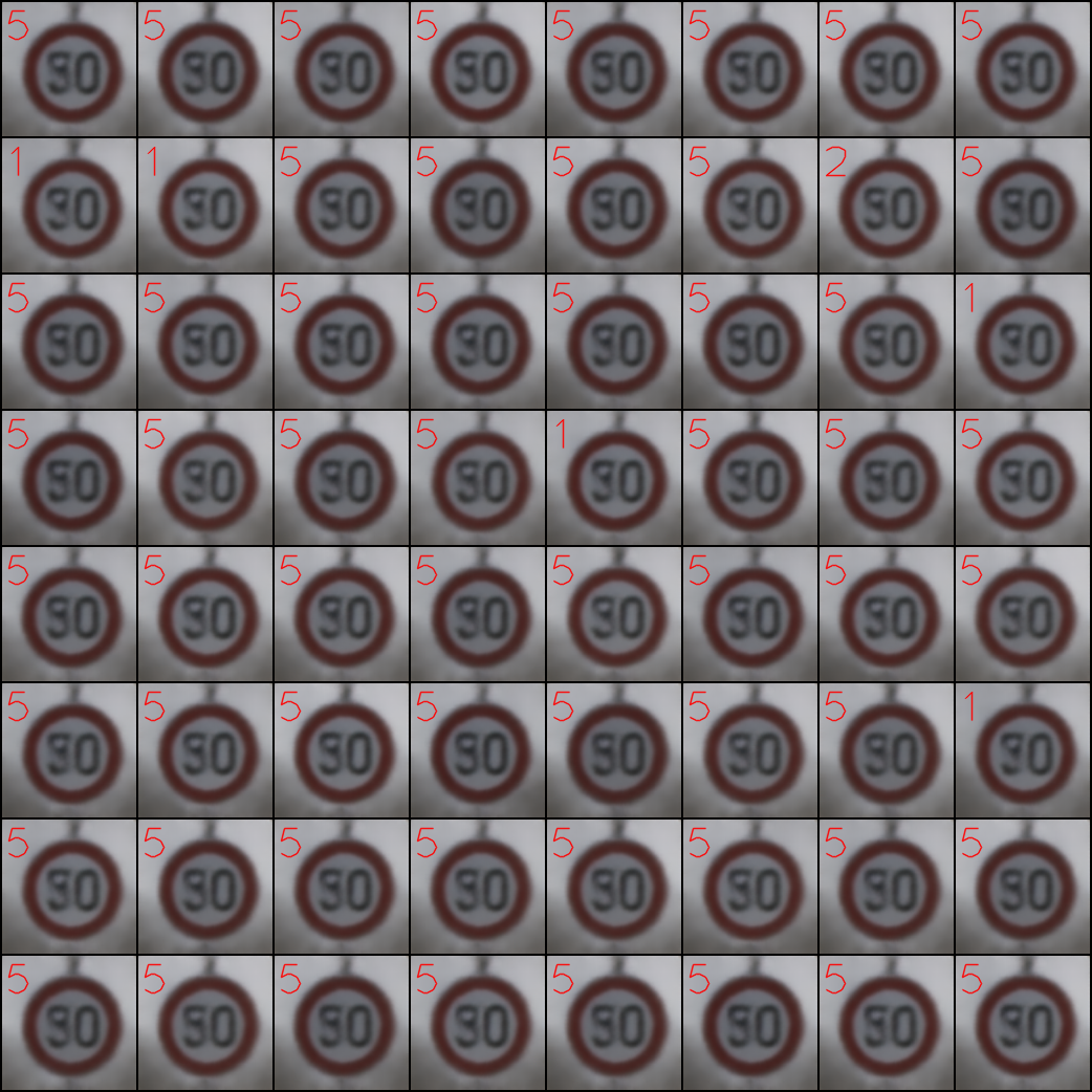
Figure 34: Annotator label $1$.

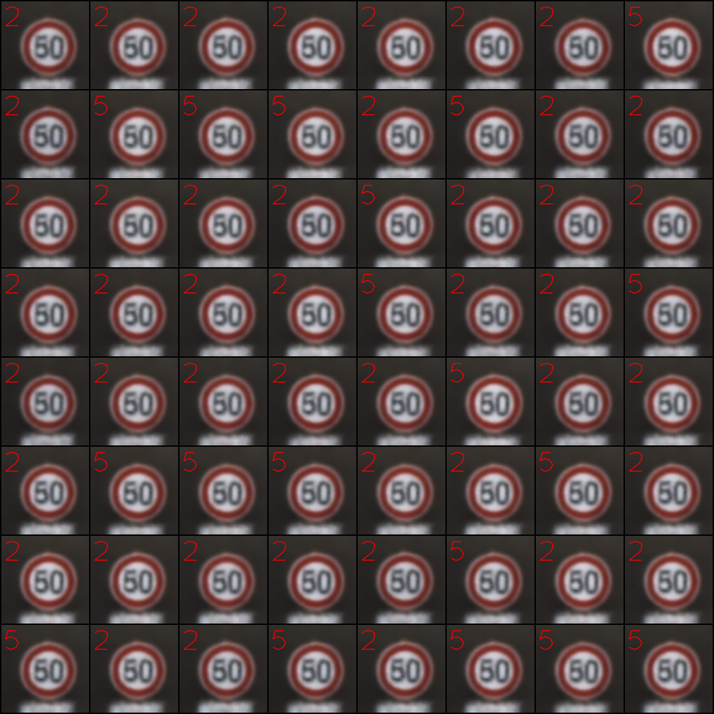
Figure 35: Annotator label $2$.

D.3 Additional samples from SVHN misclassification regions

We provide additional samples from each of the SVHN misclassification regions. The digit in the upper left hand corner is the classifier predicted label. The caption includes the Ground Truth worker labels.

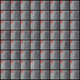
Figure 36: Annotator label $1$.

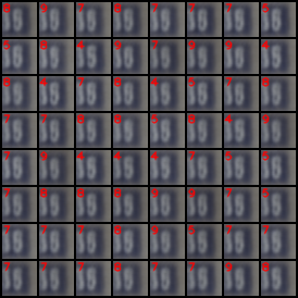
Figure 37: Annotator label $5$.

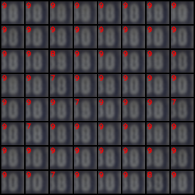
Figure 38: Annotator label $8$.

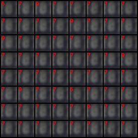
Figure 39: Annotator label $0$.

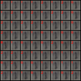
Figure 40: Annotator label $3$.

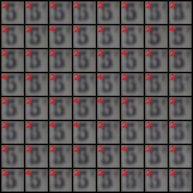
Figure 41: Annotator label $5$.

References

- Antoniou, Storkey, and Edwards (2017) Antoniou, A.; Storkey, A.; and Edwards, H. 2017. Data Augmentation Generative Adversarial Networks. International Conference on Artificial Neural Networks and Machine Learning .
- Bishop (2006) Bishop, C. M. 2006. Pattern Recognition and Machine Learning (Information Science and Statistics). Berlin, Heidelberg: Springer-Verlag. ISBN 0387310738.
- Booth et al. (2021) Booth, S.; Zhou, Y.; Shah, A.; and Shah, J. 2021. Bayes-TrEx: Model Transparency by Example. In AAAI.
- Carmon et al. (2019) Carmon, Y.; Raghunathan, A.; Schmidt, L.; Liang, P.; and Duchi, J. 2019. Unlabeled Data Improves Adversarial Robustness. In Advances in Neural Information Processing Systems (NeurIPS).
- Dumoulin et al. (2016) Dumoulin, V.; Belghazi, I.; Poole, B.; Mastropietro, O.; Lamb, A.; Arjovsky, M.; and Courville, A. 2016. Adversarially Learned Inference. ICLR .
- Engstrom et al. (2020) Engstrom, L.; Ilyas, A.; Santurkar, S.; Tsipras, D.; Steinhardt, J.; and Madry, A. 2020. Identifying Statistical Bias in Dataset Replication. ICML .
- Feldman et al. (2015) Feldman, M.; Friedler, S. A.; Moeller, J.; Scheidegger, C.; and Venkatasubramanian, S. 2015. Certifying and Removing Disparate Impact. In Proceedings of the 21th ACM SIGKDD International Conference on Knowledge Discovery and Data Mining, KDD ’15, 259–268. New York, NY, USA: Association for Computing Machinery. ISBN 9781450336642. doi:10.1145/2783258.2783311. URL https://doi.org/10.1145/2783258.2783311.
- Gardner et al. (2020) Gardner, M.; Artzi, Y.; Basmov, V.; Berant, J.; Bogin, B.; Chen, S.; Dasigi, P.; Dua, D.; Elazar, Y.; Gottumukkala, A.; Gupta, N.; Hajishirzi, H.; Ilharco, G.; Khashabi, D.; Lin, K.; Liu, J.; Liu, N. F.; Mulcaire, P.; Ning, Q.; Singh, S.; Smith, N. A.; Subramanian, S.; Tsarfaty, R.; Wallace, E.; Zhang, A.; and Zhou, B. 2020. Evaluating Models’ Local Decision Boundaries via Contrast Sets. In Findings of the Association for Computational Linguistics: EMNLP 2020, 1307–1323. Online: Association for Computational Linguistics. doi:10.18653/v1/2020.findings-emnlp.117. URL https://www.aclweb.org/anthology/2020.findings-emnlp.117.
- He et al. (2016) He, K.; Zhang, X.; Ren, S.; and Sun, J. 2016. Deep Residual Learning for Image Recognition. 2016 IEEE Conference on Computer Vision and Pattern Recognition (CVPR) 770–778.
- Higgins et al. (2017) Higgins, I.; Matthey, L.; Pal, A.; Burgess, C.; Glorot, X.; Botvinick, M. M.; Mohamed, S.; and Lerchner, A. 2017. -VAE: Learning Basic Visual Concepts with a Constrained Variational Framework. In ICLR.
- Ji, Smyth, and Steyvers (2020) Ji, D.; Smyth, P.; and Steyvers, M. 2020. Can I Trust My Fairness Metric? Assessing Fairness with Unlabeled Data and Bayesian Inference. In Advances in Neural Information Processing Systems.
- Kang et al. (2018) Kang, D.; Raghavan, D.; Bailis, P.; and Zaharia, M. 2018. Model Assertions for Debugging Machine Learning. Debugging Machine Learning Models .
- Kingma et al. (2014) Kingma, D. P.; Mohamed, S.; Jimenez Rezende, D.; and Welling, M. 2014. Semi-supervised Learning with Deep Generative Models. In Ghahramani, Z.; Welling, M.; Cortes, C.; Lawrence, N. D.; and Weinberger, K. Q., eds., Advances in Neural Information Processing Systems 27, 3581–3589. Curran Associates, Inc.
- Kumar, Sattigeri, and Fletcher (2017) Kumar, A.; Sattigeri, P.; and Fletcher, T. 2017. Semi-supervised Learning with GANs: Manifold Invariance with Improved Inference. In Guyon, I.; Luxburg, U. V.; Bengio, S.; Wallach, H.; Fergus, R.; Vishwanathan, S.; and Garnett, R., eds., Advances in Neural Information Processing Systems 30, 5534–5544. Curran Associates, Inc.
- LeCun, Cortes, and Burges (2010) LeCun, Y.; Cortes, C.; and Burges, C. 2010. MNIST handwritten digit database. ATT Labs [Online]. Available: http://yann.lecun.com/exdb/mnist 2.
- Lundberg and Lee (2017) Lundberg, S. M.; and Lee, S.-I. 2017. A Unified Approach to Interpreting Model Predictions. In Guyon, I.; Luxburg, U. V.; Bengio, S.; Wallach, H.; Fergus, R.; Vishwanathan, S.; and Garnett, R., eds., Advances in Neural Information Processing Systems 30, 4765–4774. Curran Associates, Inc. URL http://papers.nips.cc/paper/7062-a-unified-approach-to-interpreting-model-predictions.pdf.
- Milz, Rudiger, and Suss (2018) Milz, S.; Rudiger, T.; and Suss, S. 2018. Aerial GANeration: Towards Realistic Data Augmentation Using Conditional GANs. In Proceedings of the European Conference on Computer Vision (ECCV) Workshops.
- Netzer et al. (2011) Netzer, Y.; Wang, T.; Coates, A.; Bissacco, A.; Wu, B.; and Ng, A. Y. 2011. Reading Digits in Natural Images with Unsupervised Feature Learning. NIPS Workshop on Deep Learning and Unsupervised Feature Learning .
- Odena et al. (2019) Odena, A.; Olsson, C.; Andersen, D.; and Goodfellow, I. 2019. TensorFuzz: Debugging Neural Networks with Coverage-Guided Fuzzing. volume 97 of Proceedings of Machine Learning Research, 4901–4911. Long Beach, California, USA: PMLR. URL http://proceedings.mlr.press/v97/odena19a.html.
- Paszke et al. (2019) Paszke, A.; Gross, S.; Chintala, S.; Chanan, G.; Yang, E.; DeVito, Z.; Lin, Z.; Desmaison, A.; Antiga, L.; and Lerer, A. 2019. MNIST Example Pytorch URL https://github.com/pytorch/examples.
- Patel et al. (2008) Patel, K.; Fogarty, J.; Landay, J. A.; and Harrison, B. 2008. Investigating Statistical Machine Learning as a Tool for Software Development. In Proceedings of the SIGCHI Conference on Human Factors in Computing Systems, CHI ’08, 667–676. New York, NY, USA: Association for Computing Machinery. ISBN 9781605580111. doi:10.1145/1357054.1357160. URL https://doi.org/10.1145/1357054.1357160.
- Pedregosa et al. (2011) Pedregosa, F.; Varoquaux, G.; Gramfort, A.; Michel, V.; Thirion, B.; Grisel, O.; Blondel, M.; Prettenhofer, P.; Weiss, R.; Dubourg, V.; Vanderplas, J.; Passos, A.; Cournapeau, D.; Brucher, M.; Perrot, M.; and Duchesnay, E. 2011. Scikit-learn: Machine Learning in Python. Journal of Machine Learning Research 12: 2825–2830.
- Raghunathan et al. (2020) Raghunathan, A.; Xie, S. M.; Yang, F.; Duchi, J.; and Liang, P. 2020. Understanding and Mitigating the Tradeoff between Robustness and Accuracy. In III, H. D.; and Singh, A., eds., Proceedings of the 37th International Conference on Machine Learning, volume 119 of Proceedings of Machine Learning Research, 7909–7919. PMLR. URL http://proceedings.mlr.press/v119/raghunathan20a.html.
- Rajpurkar et al. (2016) Rajpurkar, P.; Zhang, J.; Lopyrev, K.; and Liang, P. 2016. SQuAD: 100,000+ Questions for Machine Comprehension of Text. In Proceedings of the 2016 Conference on Empirical Methods in Natural Language Processing, 2383–2392. Austin, Texas: Association for Computational Linguistics. doi:10.18653/v1/D16-1264. URL https://www.aclweb.org/anthology/D16-1264.
- Recht et al. (2019) Recht, B.; Roelofs, R.; Schmidt, L.; and Shankar, V. 2019. Do ImageNet Classifiers Generalize to ImageNet? volume 97 of Proceedings of Machine Learning Research, 5389–5400. Long Beach, California, USA: PMLR. URL http://proceedings.mlr.press/v97/recht19a.html.
- Ribeiro, Singh, and Guestrin (2016) Ribeiro, M. T.; Singh, S.; and Guestrin, C. 2016. “Why should I trust you?” Explaining the predictions of any classifier. In Proceedings of the 22nd ACM SIGKDD international conference on knowledge discovery and data mining, 1135–1144.
- Ribeiro et al. (2020) Ribeiro, M. T.; Wu, T.; Guestrin, C.; and Singh, S. 2020. Beyond Accuracy: Behavioral Testing of NLP Models with CheckList. In Proceedings of the 58th Annual Meeting of the Association for Computational Linguistics, 4902–4912. Online: Association for Computational Linguistics. doi:10.18653/v1/2020.acl-main.442. URL https://www.aclweb.org/anthology/2020.acl-main.442.
- Russakovsky et al. (2015) Russakovsky, O.; Deng, J.; Su, H.; Krause, J.; Satheesh, S.; Ma, S.; Huang, Z.; Karpathy, A.; Khosla, A.; Bernstein, M.; Berg, A. C.; and Fei-Fei, L. 2015. ImageNet Large Scale Visual Recognition Challenge. International Journal of Computer Vision (IJCV) 115(3): 211–252. doi:10.1007/s11263-015-0816-y.
- Sandfort et al. (2019) Sandfort, V.; Yan, K.; Pickhardt, P. J.; and Summers, R. M. 2019. Data augmentation using generative adversarial networks (CycleGAN) to improve generalizability in CT segmentation tasks. Scientific Reports 9(1): 16884. ISSN 2045-2322. doi:10.1038/s41598-019-52737-x. URL https://doi.org/10.1038/s41598-019-52737-x.
- Slack et al. (2020) Slack, D.; Hilgard, S.; Singh, S.; and Lakkaraju, H. 2020. How Much Should I Trust You? Modeling Uncertainty of Black Box Explanations. AIES .
- Song et al. (2018) Song, Y.; Shu, R.; Kushman, N.; and Ermon, S. 2018. Constructing Unrestricted Adversarial Examples with Generative Models. In Bengio, S.; Wallach, H.; Larochelle, H.; Grauman, K.; Cesa-Bianchi, N.; and Garnett, R., eds., Advances in Neural Information Processing Systems 31, 8312–8323. Curran Associates, Inc.
- Stallkamp et al. (2011) Stallkamp, J.; Schlipsing, M.; Salmen, J.; and Igel, C. 2011. The German Traffic Sign Recognition Benchmark: A multi-class classification competition. In IEEE International Joint Conference on Neural Networks, 1453–1460.
- Sudderth (2006) Sudderth, E. B. 2006. Graphical Models for Visual Object Recognition and Tracking. PhD Thesis, MIT .
- Varma et al. (2016) Varma, P.; He, B.; Iter, D.; Xu, P.; Yu, R.; Sa, C. D.; and Ré, C. 2016. Socratic Learning: Augmenting Generative Models to Incorporate Latent Subsets in Training Data. arXiv: Learning .
- Varma et al. (2017) Varma, P.; Iter, D.; De Sa, C.; and Ré, C. 2017. Flipper: A Systematic Approach to Debugging Training Sets. In Proceedings of the 2nd Workshop on Human-In-the-Loop Data Analytics, HILDA’17. New York, NY, USA: Association for Computing Machinery. ISBN 9781450350297. doi:10.1145/3077257.3077263. URL https://doi.org/10.1145/3077257.3077263.
- Wu et al. (2019) Wu, T.; Ribeiro, M. T.; Heer, J.; and Weld, D. 2019. Errudite: Scalable, Reproducible, and Testable Error Analysis. In Proceedings of the 57th Annual Meeting of the Association for Computational Linguistics, 747–763. Florence, Italy: Association for Computational Linguistics. doi:10.18653/v1/P19-1073. URL https://www.aclweb.org/anthology/P19-1073.
- Zhang et al. (2019) Zhang, H.; Yu, Y.; Jiao, J.; Xing, E.; Ghaoui, L. E.; and Jordan, M. 2019. Theoretically Principled Trade-off between Robustness and Accuracy. volume 97 of Proceedings of Machine Learning Research, 7472–7482. Long Beach, California, USA: PMLR. URL http://proceedings.mlr.press/v97/zhang19p.html.
- Zhang, Zhu, and Wright (2018) Zhang, X.; Zhu, X.; and Wright, S. J. 2018. Training Set Debugging Using Trusted Items. In AAAI.
- Zhao, Dua, and Singh (2018) Zhao, Z.; Dua, D.; and Singh, S. 2018. Generating Natural Adversarial Examples. In International Conference on Learning Representations (ICLR).