Discovery and Characterization of a Rare Magnetic Hybrid $\beta$ Cephei Slowly Pulsating B-type Star in an Eclipsing Binary in the Young Open Cluster NGC 6193

Abstract

As many as 10% of OB-type stars have global magnetic fields, which is surprising given their internal structure is radiative near the surface. A direct probe of internal structure is pulsations, and some OB-type stars exhibit pressure modes ($\beta$ Cep pulsators) or gravity modes (slowly pulsating B-type stars; SPBs); a few rare cases of hybrid $\beta$ Cep/SPBs occupy a narrow instability strip in the H-R diagram. The most precise fundamental properties of stars are obtained from eclipsing binaries (EBs), and those in clusters with known ages and metallicities provide the most stringent constraints on theory. Here we report the discovery that HD 149834 in the $\sim$5 Myr cluster NGC 6193 is an EB comprising a hybrid $\beta$ Cep/SPB pulsator and a highly irradiated low-mass companion. We determine the masses, radii, and temperatures of both stars; the $\sim$9.7 M_⊙ primary resides in the instability strip where hybrid pulsations are theoretically predicted. The presence of both SPB and $\beta$ Cep pulsations indicates that the system has a near-solar metallicity, and is in the second half of the main-sequence lifetime. The radius of the $\sim$1.2 M_⊙ companion is consistent with theoretical pre-main-sequence isochrones at 5 Myr, but its temperature is much higher than expected, perhaps due to irradiation by the primary. The radius of the primary is larger than expected, unless its metallicity is super-solar. Finally, the light curve shows residual modulation consistent with the rotation of the primary, and Chandra observations reveal a flare, both of which suggest the presence of starspots and thus magnetism on the primary.

1 Introduction

Stellar clusters and associations offer the opportunity to test and refine theories of stellar structure and evolution. Given their common distance, chemical composition, and assumed common age, clusters act as laboratories to calibrate models and physical mechanisms that must be able to simultaneously explain the observed characteristics of all cluster members. Individual stars which exhibit some form of variability, such as rotational modulation, wind variability, stellar pulsations, and/or eclipses offer an additional opportunity to derive more precise stellar information once modelled. Thus, the identification of stars which exhibit one or more forms of variability is important for the advancement of the theory of stellar structure and evolution.

OB type stars are observed to have high projected rotational velocities and are expected to rotate quickly at birth (Huang & Gies, 2006a; Daflon et al., 2007; Garmany et al., 2015). Some 20% of B stars are observed to exhibit emission in their line profiles and are classed as Be stars (Rivinius et al., 2013), a phenomenon which is associated with near-critical rotation (Porter & Rivinius, 2003), non-radial pulsations (Semaan et al., 2018), and/or binarity (Bodensteiner et al., 2020). In the absence of the transient Be phenomenon, B stars are expected to only show rotational modulation in the event that surface features are introduced by magnetic fields or chemical inhomogeneities. However, only some 10% of OB stars are observed to have global magnetic fields, making this phenomenon rare and difficult to explain theoretically (Wade et al., 2019). The incidence of stars with a detected global surface magnetic field in close binaries ($P_{orb}<10$ d) is even smaller ($<2$%; Alecian et al., 2015; Neiner et al., 2015), although chemically peculiar stars such as HgMn stars are observed to have a very high binary fraction, despite null magnetic detections (Takeda et al., 2019). Alternatively, gyrosynchrotron emission has been detected in several OB binaries, implying a magnetic field (Gagné et al., 2011).

There is a wide variety of observed pulsational variability on the upper main-sequence. OB stars are observed to exhibit either pressure (p) modes as $\beta$ Cep pulsators, or gravity (g) mode pulsations as slowly pulsating B-type stars (SPBs) driven by the $\kappa$-mechanism associated with the Fe-group opacity bump (Moskalik & Dziembowski, 1992; Dziembowski & Pamiatnykh, 1993; Pamyatnykh, 1999). Additionally, late O to early B type stars are observed to exhibit both p and g mode pulsations simultaneously as hybrid pulsators, such as $\gamma$ Peg (Handler, 2009). Theoretical instability strips for OB stars are highly sensitive to rotation, metallicity, and opacity tables (Salmon et al., 2012; Moravveji, 2016; Szewczuk & Daszyńska-Daszkiewicz, 2017), and often have trouble reproducing the total range over which pulsations are observed. With the advent of space missions, OB pulsators are being observed with an unprecedented duty-cycle, revealing an even larger diversity of pulsators that theoretical instability strips struggle to explain (Pedersen et al., 2019; Balona & Ozuyar, 2020; Burssens et al., 2020; Labadie-Bartz et al., 2020). Even in the absence of detailed modelling, the presence of pulsations in OB stars reveals a nearly Solar metallicity in order to excite modes via the $\kappa$-mechanism.

Adding to the diversity of variability, massive OB stars are also host to internal gravity waves (IGWs), which are generated by the turbulent motions at the boundary of the convective core and the radiative envelope. Such waves are theoretically predicted by simulations to produce observable photometric variability (Rogers et al., 2013; Edelmann et al., 2019) at low frequencies. The observed low-frequency excess in a large sample of CoRoT, Kepler, and TESS targets has been interpreted as being caused by IGWs (Blomme et al., 2011; Bowman et al., 2019, 2020). As the presence of IGWs is not predicted or yet observed to be dependent on metallicity, it offers an explanation for the stochastic variability often observed in massive stars that cannot be explained by sub-surface convection (Cantiello et al., 2009; Bowman et al., 2019).

The most precise estimates of stellar parameters are obtained via eclipsing binary star systems, which can produce estimates on stellar masses and radii to the percent level (Torres et al., 2010). When compared against grids of stellar models or isochrones, the age, core-mass, and other internal properties can be inferred to high precision, providing excellent evolutionary diagnostics.

Similarly, clusters can be fit with such isochrones in order to determine the age or turn-off mass of the cluster. However, clusters have been observed to exhibit features such as split main-sequences, extended main-sequence turn-offs (eMSTO), and complex chemical profiles which challenge the assumption that clusters are constituted of a single population of stars. Studies have demonstrated, however, that blue stragglers, and other split main-sequences can in part be explained by a single population, some percentage of which has undergone binary interactions, diverting stars from an otherwise apparently single star evolutionary trajectory (Beasor et al., 2019). Additionally, rapid rotation and its effects have been invoked to explain the extended main-sequence turn-off phenomenon through either photometric color changes caused by the von Zeipel effect and/or enhanced chemical mixing induced by rotational shears (Bastian et al., 2016; Dupree et al., 2017; Kamann et al., 2018; Marino et al., 2018). Alternatively, it has been shown the eMSTO phenomenon can be explained at least in part by a single population of stars with varying overshooting and envelope mixing efficiencies (Yang & Tian, 2017; Johnston et al., 2019).

However, there is not a single mechanism which can explain the diversity of observations of young massive clusters (Bastian & Lardo, 2017). Instead, many questions still remain about whether the process of star formation in clusters is a rapid process that occurs via fragmentation within two times the free fall timescale of the cluster, or if it is instead a longer process that potentially spans millions of years (Getman et al., 2014). Recently, observations have revealed that stars in the cores of young clusters are younger than stars in the halo, suggesting an outside-in formation scenario (Getman et al., 2014). Further corroboration of this scenario can be sought through the modelling of clusters which have individual stars that exhibit multiple forms of variability. To this end, clusters with several young, massive, pulsating or rotationally variable stars in eclipsing binaries offer the best means of scrutinising formation scenarios with multiple independent constraints.

In this paper, we characterise the B2V + K/MV binary HD 149834 containing an SPB / $\beta$ Cep pulsating primary. Using archival radial velocities and photometry combined with new space-based photometry from the Transiting Exoplanet Survey Satellite (TESS, Ricker et al., 2015) we perform eclipse and spectral energy distribution modelling of the system and investigate the residuals for asteroseismic and rotational signatures. Furthermore, we use the parallax and space motions from Gaia DR2 (Lindegren et al., 2018; Luri et al., 2018) to investigate the membership probability of this system. Finally, we discuss this system in an evolutionary context and conclude in Sections 5 and 6.

2 The HD 149834 Binary System: Age, Cluster Membership, and Distance Considerations

HD 149834 was identified as a single-lined spectroscopic binary (SB) by Arnal et al. (1988) in their study of likely members of the young cluster NGC 6193. More recently, HD 149834 is listed among the $\sim$550 stars considered by Cantat-Gaudin et al. (2018) as probable members of NGC 6193 (defined as having a probability of membership of 0.5 or above), based on Gaia DR2 parallaxes and proper motions. However, HD 149834 itself just barely satisfies their membership criteria, having a probability of 0.5. The Gaia color-magnitude diagram (CMD) of these stars (Figure 1) suggests an age of a few Myr, consistent with previous estimates in the literature, whereas the position of HD 149834 in the CMD is more consistent with an older age of $\sim$30 Myr.

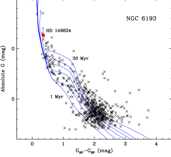
Figure 1: CMD of the parent cluster. The oldest of the MIST isochrones shown (1, 2, 3, 5, 10, 30 Myr) is the one that comes closest to the location of HD 149834.

As we will show in Section 4.2, the radial velocities reported by Arnal et al. (1988), refit by us along with the TESS photometry, yield a systemic velocity of $-{34.7\pm 1.8~{}{\rm km\thinspace s^{-1}}}$, which agrees well with the average for NGC 6193 of $-34.4\pm 2.0~{}{\rm km\thinspace s^{-1}}$ from all 18 stars observed by those authors, or $-33.2\pm 1.1~{}{\rm km\thinspace s^{-1}}$ from just the six non-variable stars in Arnal et al. (1988). This lends additional confidence that it is a true member.

At a distance of $\sim$1 kpc, the NGC 6193 cluster is part of the larger Ara OB1a association, which has other clusters also reportedly associated with it. In particular, two other clusters have been recognized as members of this association in the literature: NGC 6167, which is estimated to be 20–30 Myr (Baume et al., 2011) but at a significantly greater distance according to Gaia DR2 ($\sim$1400 pc), and NGC 6204, which has a similar distance to NGC 6193 but is estimated to be even older at $\sim$60 Myr (Kounkel et al., 2020). Accordingly, Baume et al. (2011) suggested a sequential star-formation scenario for Ara OB1 in which NGC 6167 triggered the formation of NGC 6193. But with the advent of Gaia DR2 it is now more clear that these clusters’ characteristic proper motions are also very different relative to one another, raising doubts as to whether all three clusters are in fact actually related, and in any case presents a clear case for HD 149834 being much more likely to be associated with NGC 6193 (see Fig. 2).

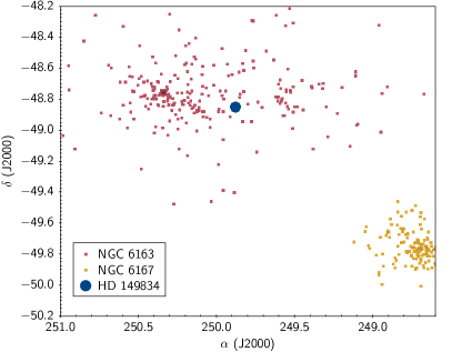
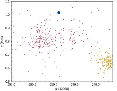
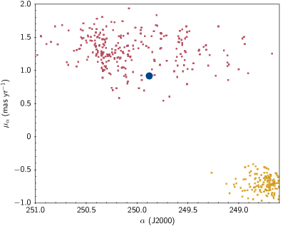
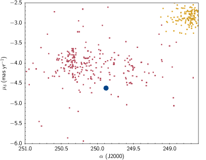
Figure 2: Astrometric and kinematic assessment of membership in NGC 6193 using the catalog from Kounkel et al. (2020).

The recent detailed analysis of stellar structures in the local Milky Way by McBride et al. (submitted) provides a more granular assessment of individual stellar ages within the region. That analysis finds that while the core of the NGC 6193 cluster has a most likely age of a few Myr, the cluster also appears to possess a “halo” of somewhat older stars, with ages of 10–15 Myr. HD 149834 appears in position and kinematics to be most likely associated with this somewhat older “halo” of NGC 6193 (see Figs. 2, 3), which could help to resolve the age tension in the CMD noted above (Figure 1).

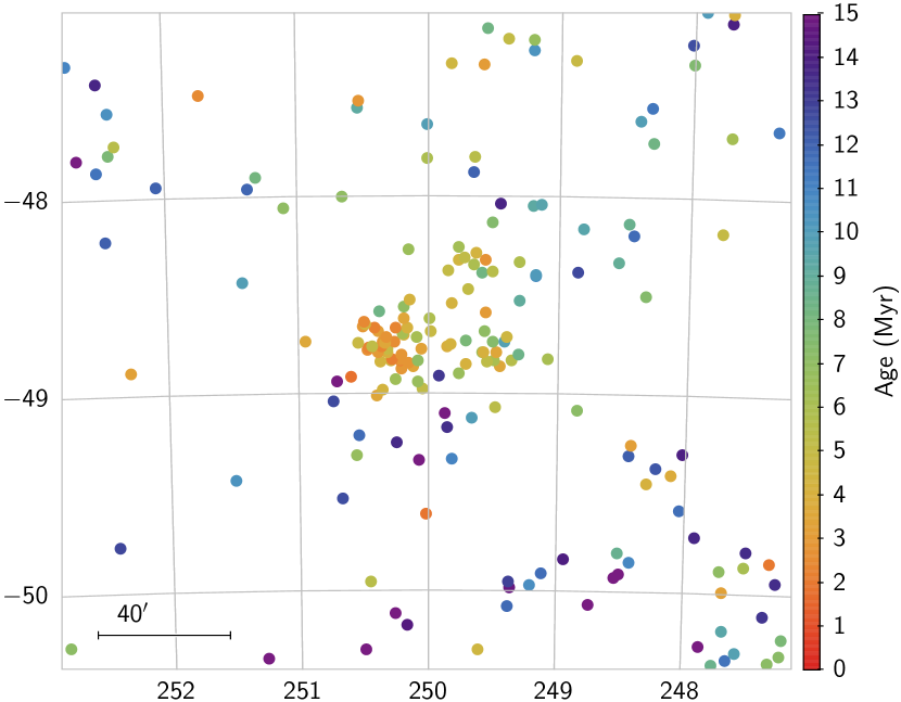
Figure 3: Map of pre-main sequence stars in the direction of NGC 6163, color coded by their estimated age, from McBride et al. (submitted).

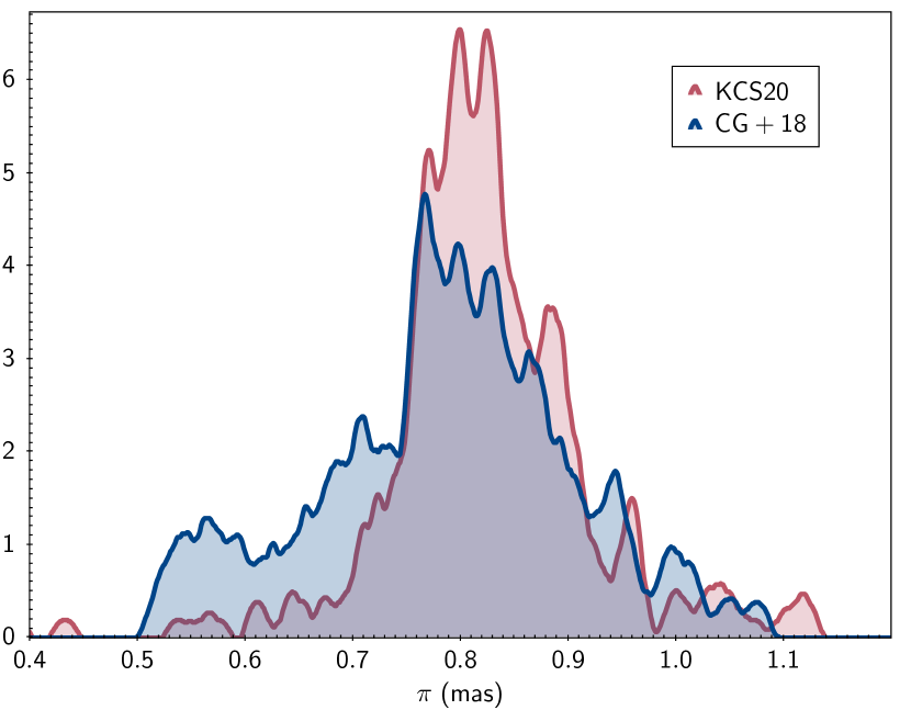
Figure 4: Distribution of parallaxes for NGC 6163 cluster, using the membership from Kounkel et al. (2020) and Cantat-Gaudin et al. (2018).

Regarding distance, even with the benefit of Gaia DR2 parallaxes the distance to NGC 6193 is somewhat uncertain due to the small parallax ($\sim$1 mas) and therefore the dependence on the choice of prior. As shown in Figure 4, the average Gaia distance to the cluster depends explicitly on which stellar members are used, how the averaging is done, and what systematics are taken into account. This leads to a choice of three distance estimates currently available: $1055\pm 70$ pc using the membership from Kounkel et al. (2020), $1302\pm 108$ pc using the Kounkel et al. (2020) algorithm on the membership from Cantat-Gaudin et al. (2018), or $1190\pm 145$ pc using the Cantat-Gaudin et al. (2018) estimate.

The Kounkel et al. (2020) analysis gives a roughly symmetric distribution that is quasi-normal and therefore lends itself to a simple $\sigma/\sqrt{N}$ estimate of the uncertainty on the mean based on a Gaussian approximation. In that case, the mean parallax for NGC 6193 is $0.835\pm 0.009$ mas. As HD 149834 is a likely member, and as the Gaia parallax measure for the star itself is significantly more uncertain, we adopt this mean cluster parallax as our estimator for the distance to HD 149834.

3 TESS Light Curve of HD 149834

TESS observed HD 149834 in its 30-min full-frame image (FFI) mode over 27 d in Sector 12, showing HD 149834 clearly to be an eclipsing binary (EB) with a primary eclipse depth of 1.4% and a secondary eclipse depth of 0.3% that could be partial or total (Figure 5). The $\sim$4.5 d orbital period is consistent with the one from the spectroscopic orbital fit by Arnal et al. (1988). The pixel mask used to extract the light curve from the TESS FFIs is shown in Figure 6.

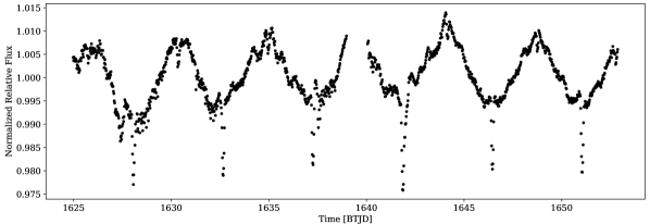
Figure 5: Raw extracted TESS FFI light curve.

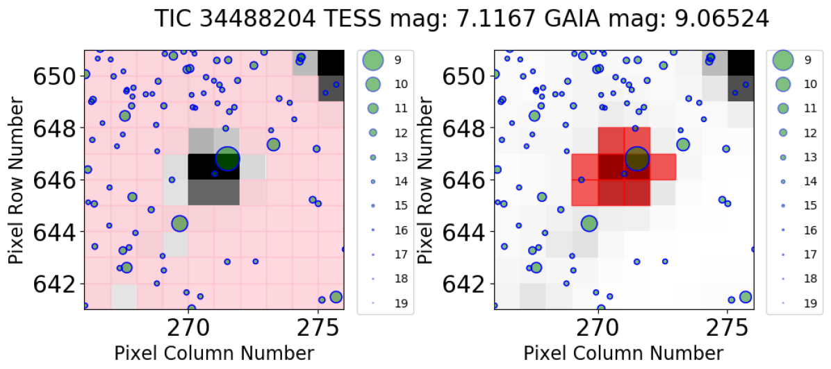
Figure 6: Cutouts of Full Frame Images from TESS Sector 12, centered on HD 149834. Nearby stars from the Gaia catalog are displayed as small circles where the size varies with Gaia magnitudes. In the left panel, the pink color represents the pixel mask to measure the background flux. In the right panel, the red color represents the pixel mask used to extract photometry from the target star.

Unfortunately there is no flux contamination estimate provided by the TESS Input Catalog (TIC; Stassun et al., 2019) because this star was not included in the TESS Candidate Target List (CTL; Stassun et al., 2019). There is one other relatively bright star in Gaia DR2, a $G=12.8$ mag star that is 38” away. That source is $\sim$3.8 mag fainter and only 1 or 2 pixels away, so its light is surely included in the extracted light curve, contributing $\sim$3%. All of the other stars that could be contributing light are fainter than $G=17$, but there are enough of them that together they add up to another $\sim$1%. We conclude that the total dilution of the HD 149834 light curve by extrinsic sources is $\approx$4%.

The light curve also exhibits out-of-eclipse variations that include a combination of instrumental systematics and true source modulations. It is important to preserve the intrinsic source modulations as they arise from reflection effects and therefore provide important constraints on the physical model solution (see Section 4). We therefore opted to detrend the light curve manually, in the following way: Data points were selected by eye near the middle of each ascending and descending branch, and they were fitted with a 5th-order polynomial. This polynomial was divided into the raw fluxes. We then ran a preliminary light curve model (see Section 4.2) and noticed that the residuals still showed systematics that were a relatively smooth function of time, particularly at the ends of the data set, most likely because the polynomial fit is not able to perform optimally at the ends of the light curve. We therefore fit a spline function to remove just the low-frequency variations in the residuals, and divided this fit into the normalized data from the previous step. This is the final photometry that we will use below in Section 4.2.

4 Analysis and Results

4.1 Spectral Energy Distribution: Initial Constraints on Stellar Properties

In order to obtain initial estimates of the component effective temperatures ($T_{\rm eff}$) and radii ($R$), we performed a multi-component fit to the combined-light, broadband spectral energy distribution (SED) of the HD 149834 system, starting with the $T_{\rm eff}$ and $R$ estimates for the primary star from the spectroscopic study of Huang & Gies (2006a). The resulting $T_{\rm eff}$ and $R$ were iteratively updated based on the joint light-curve and radial-velocity model (Section 4.2) until a final satisfactory SED fit was produced.

As shown in Figure 7 (black curve), the SED from 0.3 $\mu$m to 10 $\mu$m can be very well fit by a single component with $T_{\rm eff}=21467\pm 246$ K, $\log g=3.95\pm 0.15$, and [Fe/H]$\,\approx\,$0 as reported from a previous spectroscopic analysis in the literature (Huang & Gies, 2006b), with a best-fit extinction of $A_{V}=1.4\pm 0.1$ (consistent with other determinations of the reddening of this cluster; e.g., Rangwal et al., 2017).

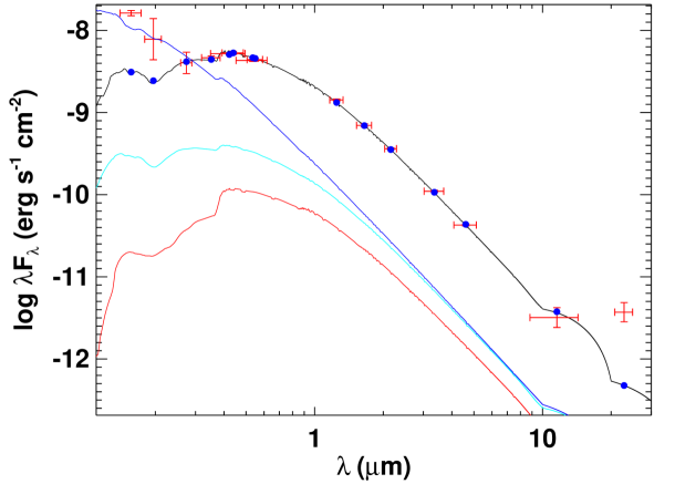
Figure 7: Multi-component fit to the combined-light SED of HD 149834. Observed fluxes are represented as red symbols (horizontal error bars represent filter widths); blue symbols are the corresponding model fluxes. The black curve is a single-source fit using spectroscopic $T_{\rm eff}=21500$ K, [Fe/H]=0, and best-fit $A_{V}=1.4$. Other curves are attempts to represent the secondary in different ways; the only acceptable choice given the observational constraints on the flux ratio is the red curve with $T_{\rm eff}=$ 13 000 K and same $A_{V}$ as above; see the text.

Interestingly, there is an apparent excess in the UV. In principle this could be due to activity on the low-mass companion star; young low-mass stars have ubiquitous UV excess even after they stop accreting. Alternatively, the UV excess could suggest an additional hot source in the system. However, adding a second component cannot reproduce that excess if the same $A_{V}$ is applied. For example, adopting the secondary star’s radius determined from the light curve analysis (Sec. 4.2), we can reproduce the UV excess with a secondary $T_{\rm eff}=25\,000$ K (the dark blue curve in Fig. 7), however this requires zero extinction. Reddening it by the same $A_{V}$ as above yields the light blue curve, which predicts gives a flux ratio in the TESS band of 6.9%, much too large for the $\sim$2.5% flux ratio that is required by the light curve analysis (Section 4.2).

Therefore the UV excess is not easily explained, and we note also evidence for an excess at 20 $\mu$m. We are able to reproduce the $\sim$2.5% flux ratio in the TESS band with the same $A_{V}$ applied if we instead adopt $T_{\rm eff}=$13 000 K (red curve in Fig. 7). Such a faint companion would require extraordinarily strong intrinsic UV emission to produce the observed UV excess, some 5 orders of magnitude over photospheric (see Fig. 7). Thus the origin of the UV emission, if real, remains unclear (but see Sec. 4.4 regarding observed X-ray emission in the system).

Most importantly, the SED analysis provides robust initial constraints on the properties of the stars that we can utilize in the full solution below (Sec. 4.2). Adopting the parallax estimated in Sec. 2 and correcting for the 0.029 mas systematic offset of the Gaia DR2 parallaxes reported by the Gaia mission, we obtain via the bolometric flux from the SED fit an estimate for the primary star radius: $R_{1}=4.96\pm 0.13$ R_⊙. This radius, together with the spectroscopic $\log g$, then gives an estimate for the primary mass of $M_{1}=8.1\pm 1.3$ M_⊙.

4.2 TESS Light Curve Analysis: Detailed Determination of Stellar Properties

We used the detrended TESS photometry described in Section 3, along with its internal uncertainties, to perform a light curve analysis of HD 149834 using the eb code of Irwin et al. (2011), which is based on the Nelson-Davis-Etzel binary model (Etzel, 1981; Popper & Etzel, 1981) underlying the popular EBOP program by those authors. This model is adequate for well-detached systems such as HD 149834, having nearly spherical stars. The main adjustable parameters we considered are the orbit period ($P$), a reference epoch of primary eclipse ($T_{0}$, which in this code is strictly the time of inferior conjunction), the central surface brightness ratio in the TESS bandpass ($J\equiv J_{2}/J_{1}$), the brightness level at the first quadrature ($m_{0}$), the sum of the relative radii normalized by the semimajor axis ($r_{1}+r_{2}$), the cosine of the inclination angle ($\cos i$), and the eccentricity parameters $e\cos\omega$ and $e\sin\omega$, with $e$ being the eccentricity and $\omega$ the longitude of periastron. The radius ratio ($k\equiv r_{2}/r_{1}$), normally also an adjusted parameter in light curve solutions, was instead derived at each iteration of our analysis based on other information, as we explain below. In order to account for the flux contamination in the TESS aperture described in Sec. 3, we also solved for the third light parameter $\ell_{3}$, defined such that $\ell_{1}+\ell_{2}+\ell_{3}=1$, in which $\ell_{1}$ and $\ell_{2}$ for this normalization are taken to be the light at first quadrature.

A linear limb-darkening law was adopted for this work, with coefficients for solar metallicity taken from the tabulation by Claret (2017) for the TESS band, interpolated to the temperatures and surface gravities of the stars based on our final analysis. The same source was used for the gravity darkening coefficients. Due to the large difference in temperature between the components indicated earlier, there is a strong reflection effect in the light curve caused by the energy from the primary being re-radiated toward the observer by the cooler secondary star, with a strength controlled by the reflection coefficient of the secondary, $\eta_{2}$ (Etzel, 1981). We therefore solved for this additional parameter, while leaving the corresponding coefficient for the primary set to zero, as its impact is negligible. We accounted for the finite time of integration of the TESS photometry by oversampling the model light curve and then integrating over the 30-minute duration of each cadence prior to the comparison with the observations (see Gilliland et al., 2010; Kipping, 2010).

In addition to the photometry, we incorporated the radial velocities of Arnal et al. (1988) directly into the analysis together with their reported uncertainties, solving for the velocity semiamplitude of the primary star ($K_{1}$) and the center-of-mass velocity of the system ($\gamma$). The use of these older data extends the time base significantly to nearly 35 years, thereby improving the period determination.

The solution was carried out within a Markov chain Monte Carlo (MCMC) framework using the emcee code of Foreman-Mackey et al. (2013), with 100 walkers of length 15,000 each, after discarding the burn-in. We adopted uniform priors over suitable ranges for most parameters mentioned above, and a log-uniform prior for $\eta_{2}$. The prior for $\ell_{3}$ was assumed to be Gaussian, with a mean value of 4% as derived in Section 3, and a standard deviation of 1%. Convergence of the chains was checked visually, requiring also a Gelman-Rubin statistic of 1.05 or smaller for each parameter (Gelman & Rubin, 1992). The relative weighting between the photometry and the radial velocities was handled by including additional adjustable parameters $f_{\rm phot}$ and $f_{\rm RV}$ to rescale the observational errors. These multiplicative scale factors were solved for self-consistently and simultaneously with the other orbital quantities (see Gregory, 2005), adopting log-uniform priors for both.

As we only have radial velocities for the primary star, an estimate of the mass $M_{1}$ of that component is required before we can derive the absolute the mass and radius of the secondary. The spectroscopic study of Huang & Gies (2006b) reported an estimate of the surface gravity for the primary of $\log g_{1}=3.955\pm 0.023$, although they considered 0.15 dex to be a more realistic estimate of the uncertainty. We adopt this more conservative error here. The $\log g$ value together with the radius estimate $R_{1}$ for that star from our SED fit above yields the necessary information to infer $M_{1}$. In order to propagate the uncertainties more accurately to the radius and mass of the secondary, we chose to add $\log g_{1}$ and $R_{1}$ as adjustable parameters in our solution, constrained by Gaussian priors given by the measured values and corresponding errors of those two quantities. At each iteration we then solved for the mass and radius of the secondary, which immediately provides the radius ratio $k\equiv r_{2}/r_{1}=R_{2}/R_{1}$ needed to model the light curve.

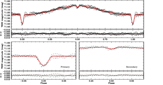
Figure 8: Final detrended TESS photometry with our model fit shown in red.

The results of our analysis for HD 149834 are presented in Table 1, in which we report the mode of the posterior distribution for each parameter. Posterior distributions of the derived quantities listed in the bottom section of the table were constructed directly from the MCMC chains of the adjustable parameters involved. Our adopted lightcurve model along with the TESS observations are seen in Figure 8, with residuals shown at the bottom of each panel.

Table 1: Results From our MCMC Analysis of HD 149834

Parameter	Value	Prior
$P$ (days)	$4.595701^{+0.000035}_{-0.000038}$	[4, 5]
$T_{0}$ (HJD$-$2,400,000)	$58641.8547^{+0.0010}_{-0.0011}$	[58641, 58642]
$J$	$0.21^{+0.23}_{-0.11}$	[0.0, 1.0]
$r_{1}+r_{2}$	$0.249^{+0.014}_{-0.016}$	[0.01, 0.60]
$\cos i$	$0.224^{+0.015}_{-0.017}$	[0, 1]
$e\cos\omega$	$-0.0009^{+0.0014}_{-0.0017}$	[$-$1, 1]
$e\sin\omega$	$-0.037^{+0.012}_{-0.014}$	[$-$1, 1]
$m_{0}$ (mag)	$7.12210^{+0.00014}_{-0.00020}$	[7.0, 7.5]
$\eta_{2}$	$0.00777^{+0.00012}_{-0.00011}$	[$-15$, $-1$]
$\ell_{3}$	$0.0399^{+0.0103}_{-0.0095}$	$G(0.04,0.01)$
$\gamma$ (km s-1)	$-34.7^{+1.7}_{-1.8}$	[$-50$, $-20$]
$K_{1}$ (km s-1)	$22.5^{+1.9}_{-2.2}$	[10, 50]
$f_{\rm phot}$	$8.54^{+0.19}_{-0.15}$	[$-5$, 5]
$f_{\rm RV}$	$2.17^{+0.57}_{-0.26}$	[$-5$, 5]
$R_{1}$ ($R_{\sun}$)	$4.96^{+0.12}_{-0.14}$	$G(4.96,0.13)$
$\log g_{1}$ (cgs)	$4.040^{+0.034}_{-0.029}$	$G(3.955,0.15)$
Derived quantities
$r_{1}$	$0.1940^{+0.0035}_{-0.0054}$	$\cdots$
$r_{2}$	$0.0468^{+0.0231}_{-0.0065}$	$\cdots$
$k\equiv r_{2}/r_{1}$	$0.235^{+0.129}_{-0.026}$	$\cdots$
$i$ (degrees)	$77.07^{+1.02}_{-0.86}$	$\cdots$
$e$	$0.037^{+0.012}_{-0.014}$	$\cdots$
$\omega$ (degrees)	$91.0^{+3.7}_{-1.8}$	$\cdots$
$K_{2}$ (km s-1)	$251.6^{+11.0}_{-7.4}$	$\cdots$
$M_{1}$ ($M_{\sun}$)	$9.71^{+1.22}_{-0.81}$	$\cdots$
$M_{2}$ ($M_{\sun}$)	$0.858^{+0.123}_{-0.096}$	$\cdots$
$q\equiv M_{2}/M_{1}$	$0.0874^{+0.0093}_{-0.0079}$	$\cdots$
$R_{2}$ ($R_{\sun}$)	$1.16^{+0.64}_{-0.13}$	$\cdots$
$\log g_{2}$ (cgs)	$4.11^{+0.23}_{-0.24}$	$\cdots$
$a$ ($R_{\sun}$)	$25.57^{+0.97}_{-0.76}$	$\cdots$

Note. — The values listed correspond to the mode of the respective posterior distributions, and the uncertainties represent the 68.3% credible intervals. All priors are uniform over the specified ranges, except those for $\eta_{2}$, $f_{\rm phot}$, and $f_{\rm RV}$, which are log-uniform, and the priors for $R_{1}$, $\log g_{1}$, and $\ell_{3}$, which are Gaussian with mean and standard deviations as indicated by the notation $G({\rm mean},\sigma)$.

Due to the reflection effect the light ratio between the components of HD 149834 changes by a factor of about 1.9 as a function of orbital phase. This is illustrated in Figure 9. Our model radial-velocity curve with the observations of Arnal et al. (1988) is shown in Figure 10, indicating a center-of-mass velocity consistent with membership in NGC 6193, as mentioned earlier.

Figure 9: Light ratio between the secondary and primary components of HD 149834 as a function of orbital phase, showing the significant changes due to the reflection effect.

Figure 10: Radial velocity measurements of Arnal et al. (1988) along with our model fit. Residuals are displayed at the bottom.

4.3 HR Diagram: Evolutionary Analysis

Figure 11 depicts the two components of the HD 149834 system in the mass-radius and $T_{\rm eff}$-radius planes, compared to the PARSEC model isochrones. In the mass-radius plane, the secondary appears roughly as expected for the nominal cluster age of 5 Myr, whereas the primary appears too large for that age; it appears slightly evolved with an inferred age of $\sim$20 Myr.

In the $T_{\rm eff}$-radius plane, both components can be reasonably well fit by the 20 Myr isochrone (note the very large uncertainty on the secondary $T_{\rm eff}$ due to the large uncertainty on $J$ from the light curve analysis). However, this is misleading because the secondary’s measured mass of $\sim$0.86 M_⊙ should place it at a much cooler $T_{\rm eff}$.

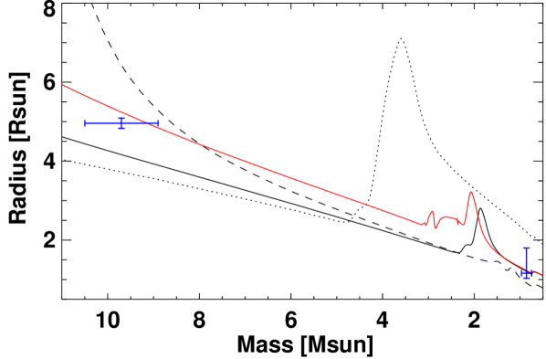
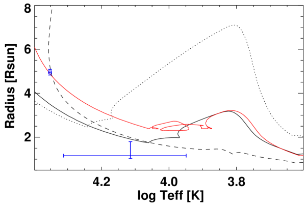
Figure 11: Mass-radius (top) and $T_{\rm eff}$-radius (bottom) representations of the HD 149834 primary and secondary (blue error bars). Black curves are PARSEC isochrones at solar metallicity for ages of 1 Myr (dotted), 5 Myr (solid), and 20 Myr (dashed). Red curves are the same but for [M/H] = $+$0.7 at the nominal cluster age of 5 Myr.

It is possible to explain both stars in the mass-radius diagram at about 5 Myr with a super-solar metallicity; however the required metallicity is quite high at +0.7 (red curve). Unfortunately, there is no reliable literature estimate of the metallicity for HD 149834. Nonetheless, given all of the available evidence, we prefer this solution as both stars are then most consistent with the nominal age of the NGC 6193 cluster, and the anomalously high $T_{\rm eff}=13\,000^{+7500}_{-4000}$ K for the secondary attributed to its extremely high irradiation from the primary.

4.4 Chandra X-ray Light Curve: Activity

Wolk et al. (2008) observed HD 149834 (Source 174 in their study) using Chandra for $\sim 25$ hours, starting at UT 2:37 on 2004 October 25. They identified HD 149834 as a flare source using Bayesian blocks (Scargle, 1998) with variability detected at 95% significance; its light curve is plotted in Figure 12. Based on the ephemeris we determine in Section 4.2 (see Table 1), the Chandra observations span orbital phases 0.57–0.80, with a formal uncertainty of less than 0.01. However, the possibility of multiple period aliases makes the uncertainty likely larger.

Taken at face value, the ephemeris suggests that the observed flare occurs near phase 0.75, when HD 149834 B is accelerating towards us. In any case, along with the UV excess seen in the SED (Sec. 4.1 and Fig. 7), this flare may be a signature of activity from HD 149834. An actual detection of the secondary eclipse in the X-ray light curve would have implicated HD 149834 B as the source.

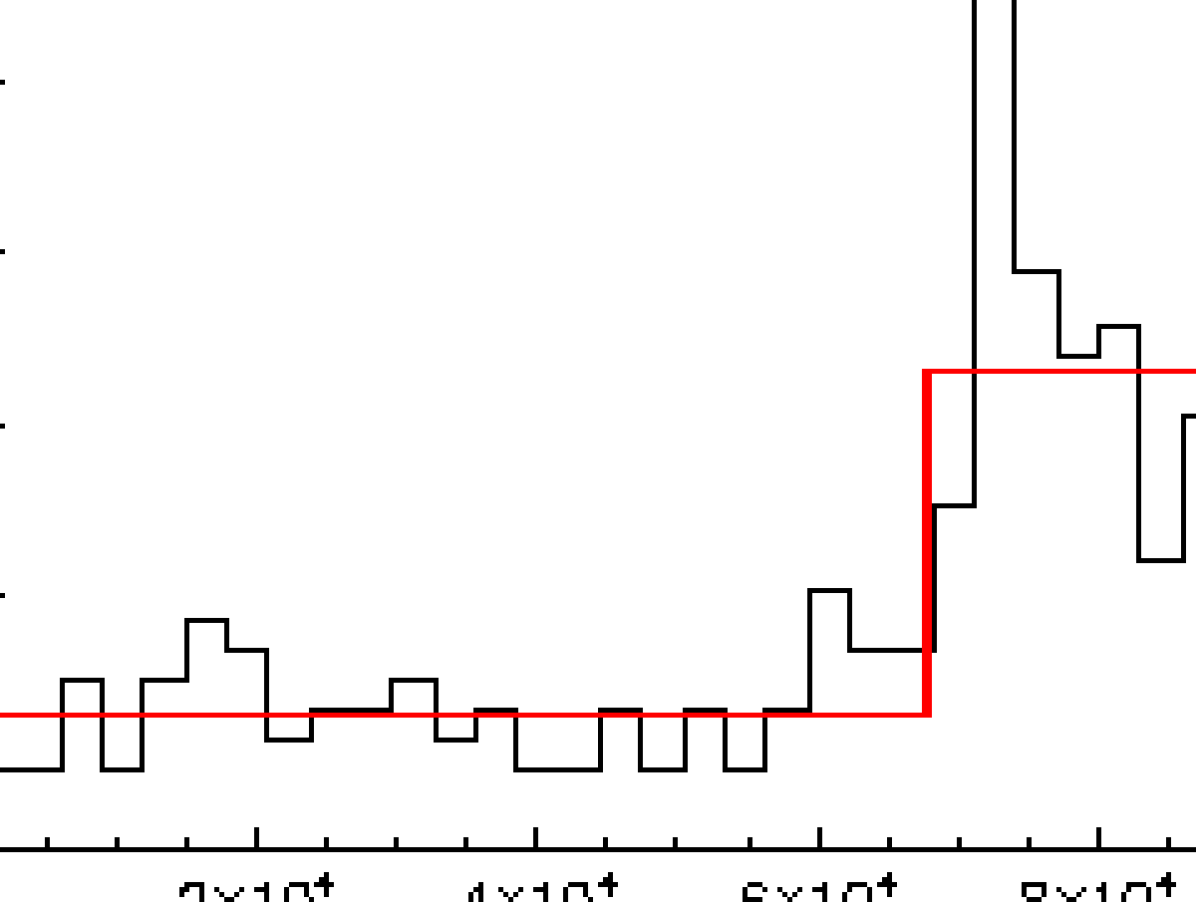
Figure 12: Chandra X-ray light curve (black) and Bayesian block (red) for HD 149834 (S. Wolk, private communication).

4.5 TESS Residuals: Pulsations and Rotation

Following the subtraction of the best fit model determined in Section 4.2, we investigate the residuals to determine if any remaining signal is present. By comparing the residuals (black) with the background (grey) in Fig. 13, we see that the variation induced by the Earth-shine events is still present, despite the detrending. This event occurs twice, separated by approximately 16 days.

We subjected the residuals to an iterative pre-whitening analysis using the pythia python package wherein we calculate a Lomb-Scargle periodogram of the residuals, identify the frequency with the highest amplitude, and fit a sinusoid to the data to determine the optimal frequency, amplitude, and phase of that signal. The optimized signal is then subtracted, and the signal-to-noise ratio (S/N) of signal is computed by dividing the amplitude of the optimized sinusoid by the average noise level of the periodogram of the residuals after subtraction of the identified signal within a window of 3 d^-1. This process is repeated until an extracted peak is found to have S/N $<$ 3.5 At the end of this process, we simultaneously fit all frequencies, amplitudes, and phases to the original data, and re-calculate the S/N according to the new residuals. We retain all independent frequencies with S/N $>$ 4 (Breger et al., 1993). Following Breger et al. (1999) and considering the average uncertainty of the extracted frequencies, we retain any combination frequency with S/N $>$ 3.3.

Following Degroote et al. (2009), after extraction we filter for close frequencies defined as $\delta f\leq 2.5f_{\rm R}$, and keep the frequency which has the higher amplitude. Here, the Rayleigh frequency, $f_{\rm R}\approx 0.036$ d^-1 is the inverse of the time-base of the TESS lightcurve. We identify 8 frequencies, listed in Table 2, two of which are combination frequencies or orbital harmonics, within the frequency uncertainties. The full Lomb-Scargle periodogram of the binary subtracted residuals is shown in Fig. 14, where 4 and 3.3 times the average noise level are depicted by the dashed-dotted and dotted grey lines, respectively. Furthermore, we identify $f_{7}$ as matching both the 34th orbital harmonic. The residuals after binary subtraction and optimised sinusoid model comprised of the frequencies in Table 2 are shown in Fig. 13 in black and red, respectively.

Additionally, we note that the mass of the primary is within the range of stars that are expected to exhibit internal gravity waves (IGWs) excited at the boundary of the convective core. Both 2D and 3D hydrodynamical simulations demonstrate that IGWs observationally manifest as a low-frequency excess and/or as resonantly excited g modes in photometry (Rogers et al., 2013; Bowman et al., 2019; Lecoanet et al., 2019; Edelmann et al., 2019; Horst et al., 2020). Given the observed low-frequency excess in the periodogram of the residuals of HD 149834, we fit periodogram according to Blomme et al. (2011); Bowman et al. (2019), with:

$$\alpha_{\nu}=\frac{\alpha_{0}}{1+\left(\nu/\nu_{\rm char}\right)^{\gamma}}+W,$$ (1)

to determine the parameters of the background profile. Here, $\alpha_{0}$ and $W$ are the amplitude at $\nu=0$ and the white noise, respectively. $\gamma$ controls the slope of the profile, and $\nu_{\rm char}$ is the characteristic frequency, at which the profile has half of its initial value. We find that the low-frequency excess is best described with $W=28.6~{}\mu$mag, $\alpha_{0}=78.8~{}\mu$mag, $\gamma=2.34$, and $\nu_{\rm char}=3.32$ d^-1. The best fit profile is plotted in red in Fig. 14.

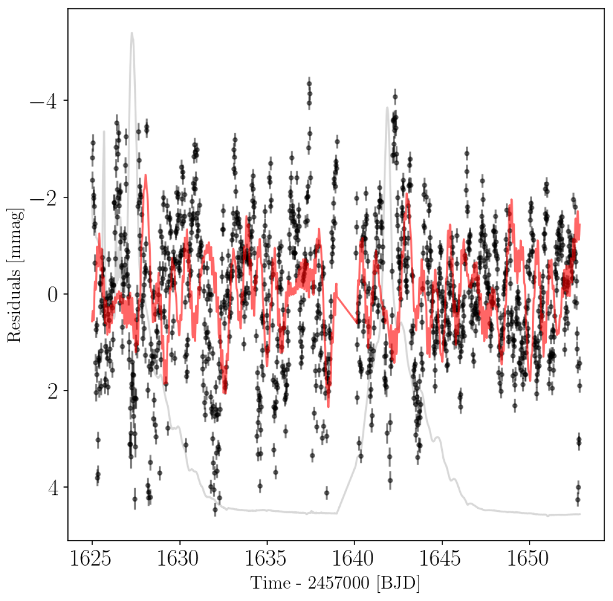
Figure 13: Residuals (black) and pulsation model (red) including all significant frequencies listed in Table 2. Re-scaled background lightcurve in grey.

	Frequency	Amplitude	SNR	Comment
	d-1	mmag
$f_{1}$	$0.329\pm 0.0171$	$0.56\pm 0.00$	5.3
$f_{2}$	$0.527\pm 0.0216$	$0.44\pm 0.00$	4.3
$f_{3}$	$0.618\pm 0.0282$	$0.34\pm 0.00$	3.3	$f_{6}-f_{4}$
$f_{4}$	$0.806\pm 0.0235$	$0.41\pm 0.00$	4.0
$f_{5}$	$1.201\pm 0.0158$	$0.60\pm 0.00$	6.2
$f_{6}$	$1.390\pm 0.0276$	$0.35\pm 0.00$	4.0
$f_{7}$	$7.373\pm 0.0662$	$0.14\pm 0.00$	3.5	$34f_{\rm orb}$
$f_{8}$	$7.969\pm 0.0459$	$0.21\pm 0.00$	5.2

Table 2: Extracted and filtered frequencies from iterative pre-whitening analysis.

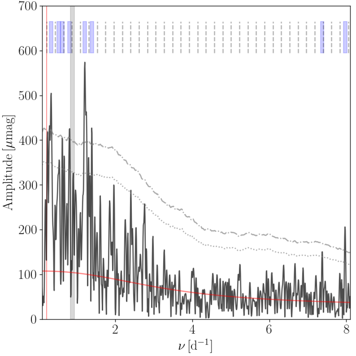
Figure 14: Lomb-Scargle periodogram of the residuals after subtraction of the binary model. Grey dash-dotted and grey dotted lines indicate the a factor 3.5 and 3 times the noise level, respectively. Grey vertical region denotes the rotational period calculated using the values in Table 1. Vertical blue regions denote the extracted frequencies and their uncertainties, and vertical dashed grey lines denote orbital harmonics. Red profile is the red-noise profile fit to the periodogram of the residuals after iterative prewhitening.

5 Discussion

5.1 Cluster membership and age considerations

The kinematics, distance, and age of HD 149834 are consistent with it being a member of NGC 6193. The mass of the primary makes it one of the most massive members of this cluster. HD 149834 A is at the mass limit where a star is predicted to produce a supernova at the end of its life, depending on the rotational and internal chemical mixing history of the star. Notably, HD 149834 is not the most massive system in NGC 6193. There are two massive multiple systems, HD 150135 (a binary; Sota et al., 2014) and HD 150136 (a triple; Mahy et al., 2012; Sana et al., 2012; Mahy et al., 2018), both of which are confirmed luminous X-ray sources (Skinner et al., 2005). Using a combination of radial velocities (Arnal et al., 1988; Mahy et al., 2012; Sana et al., 2013; Cox et al., 2017), photometry, and long time-base interferometry (Sanchez-Bermudez et al., 2013; Le Bouquin et al., 2017), Mahy et al. (2018) found HD 150136 to be comprised of a $\sim 42.8+29.5$ M_⊙ close inner binary and $\sim 15.5$ M_⊙ wide tertiary. Furthermore, they determine a common age of the components to be 0–2 Myr, which is about half the nominal age estimate of the cluster.

As mentioned in Section 4.3, there is some tension between the metallicity and age of HD 149834, which may be explained either by the anomalously hot secondary or by the system being a member of the cluster halo, which is estimated to be slightly older than the cluster core. This, however, puts more contention between the age estimates of HD 150136 and HD 149834. Alternatively, such an age gradient between halo and core members of the same cluster has been observed in other young clusters and is evidence for outside-in star formation scenarios (Getman et al., 2014).

5.2 Coherent and stochastic oscillations in HD 149834 A

Of the 8 extracted signals, 6 are independent and 2 are low-order linear combination frequencies or harmonics. The extracted frequencies occur in two distinct frequency regimes. The single independent high frequency we extracted is consistent with the expected frequency range for p mode pulsations in $\beta$ Cep stars. Those lower frequency peaks we extracted occur in a frequency regime that is consistent with rotational modulation, low-frequency instrumental noise, low-order heat-driven p and g modes, as well as IGWs and pulsation modes resonantly excited by IGWs. The 9.7 M_⊙ primary is situated in the mass range where both g and p mode pulsations are theoretically expected to be excited (Walczak et al., 2015; Moravveji, 2016; Szewczuk & Daszyńska-Daszkiewicz, 2017).

Furthermore, the values we determined for $\gamma$ and $\nu_{\rm char}$ are consistent with the values expected for IGWs in massive stars as determined from simulations (Edelmann et al., 2019; Horst et al., 2020) as well as a large sample of OB type stars observed by Kepler, CoRoT, and TESS (Bowman et al., 2020). While subsurface convection has been proposed to generate similar signals (Cantiello et al., 2009; Lecoanet et al., 2019), it is expected to produce low-frequency profiles with significantly different values of $\gamma$, i.e., $\gamma\geq 3.5$ (Couston et al., 2018), than those expected to be produced by IGWs, i.e., $1\leq\gamma\leq 3.5$ (Edelmann et al., 2019). To this end, we find that the low-frequency power excess observed in the TESS data of HD 149834 to be consistent with the presence of IGWs in the massive primary.

There is much debate concerning the theoretical instability strips of SPB and $\beta$ Cep pulsators. Several studies have demonstrated that the edges of the instability strips can change drastically depending on the choice of metallicity (Daszyńska-Daszkiewicz et al., 2013), opacity table (Salmon et al., 2012; Walczak et al., 2015; Moravveji, 2016), and rotation rate (Szewczuk & Daszyńska-Daszkiewicz, 2017). One of the most important implications of this is that these stars require a sufficiently high (nearly solar) metallicity in order to excite pulsations via the $\kappa$-mechanism. Furthermore, Southworth et al. (2020) have demonstrated that in addition to the canonical heat-driven pulsations present in $\beta$ Cep star, B-type stars in binaries can also host tidally perturbed oscillations. However, we note that due to the low amplitudes expected in such pulsations, we are not likely to observe them with the current data set. To further complicate this picture, both 2D and 3D simulations have demonstrated that IGWs can resonantly excite p and g modes (Edelmann et al., 2019; Ratnasingam et al., 2020). With the current frequency resolution, however, we are not able to distinguish between coherently driven modes excited via the $\kappa$-mechanism and modes resonantly excited via IGWs.

The evolutionary status of the primary is consistent with the instability regions of both low-order $\beta$ Cep type p and g modes, as well as high-order SPB like g mode pulsations. (Godart et al., 2017). Depending on the choice of metallicity, opacity enhancement, and / or rotation rate, p mode pulsations are only predicted toward the middle to latter half of the main-sequence. Based on the evolutionary stage of the primary, the detection of p modes is consistent with low overtone non-radial p modes. Additionally, both p and g modes are expected to be shifted to higher frequencies in the presence of rapid rotation, making the observed g and p mode pulsations consistent with low-overtone non-radial oscillations.

Burssens et al. (2020) recently reported on the detection of SPB, $\beta$ Cep, and hybrid pulsators observed in the TESS 2 minute cadence data. Of the 98 stars in their sample, only 9 are eclipsing binaries, and only three are hybrid pulsators. Interestingly, none of the EBs are observed to host hybrid pulsating stars. To date, there are only a handful of hybrid SPB / $\beta$ Cep stars known in binary systems (see e.g., Degroote et al., 2012; González et al., 2019) and a handful of either SPB or $\beta$ Cep pulsators in systems that are eclipsing, (see e.g., Freyhammer et al., 2005; Tkachenko et al., 2014; Jerzykiewicz et al., 2015). While there are several known $\beta$ Cep or SPB pulsating stars in clusters (Balona & Shobbrook, 1983; Handler et al., 2007; Saesen et al., 2013; Moździerski et al., 2019), no hybrid pulsating SPB/$\beta$ Cep stars in EBs have been identified in clusters to date. Although, this is likely a consequence of data quality and duty cycle, rather than a physical deficiency.

5.3 Rotational signal

In addition to the pulsational variability, any rotational modulation is also expected to occur in the low-frequency regime. To test this, we consider two scenarios: i) rotation synchronous with the orbital period, i.e. $f_{\rm rot}=0.21759\pm 0.00001$ d^-1 and ii) rotation consistent with the projected rotational velocity measured by Huang & Gies (2006b), $v\sin i=216\pm 11$ km s^-1, i.e. $f_{\rm rot}=0.88\pm 0.05$ d^-1, using the values for $R_{1}$ and $i$ from Table 1. Both of these values are plotted in Fig. 14, with the rotation rate derived assuming synchronous rotation in red and the rotation frequency derived from Huang & Gies (2006b) in grey. There is no significant signal remaining in the residuals at the orbital frequency. However, $f_{4}$ in Table 2 agrees with the derived rotation rate from Huang & Gies (2006b), within $2\sigma$. Assuming $f_{\rm rot}=0.88\pm 0.05$ d^-1, we find $v/v_{crit}=44\pm 4$%, using the values from Table 1. The rotation velocity of the primary is consistent with the observed distribution of projected rotational velocities of B-stars in clusters (Garmany et al., 2015).

The potential identification of a photometric signal associated with the rotation rate raises further questions. Given the stably stratified radiative envelope predicted in a typical 9.7 M_⊙ star, star-spots are not expected. Instead, if a surface inhomogeneity is observed, it could be caused by a strong magnetic field that induces surface chemical peculiarity (Alecian et al., 2015; David-Uraz et al., 2019).

An alternative mechanism for inducing photometric variability that coincides with the rotation period is rotationally modulated clumpy winds, as has been observed by Aerts et al. (2018). To frame the context of HD 149834, only about $\sim 10$% of OB stars are observed to have a detectable surface magnetic field. Furthermore, whereas non-magnetic chemically peculiar late B-type stars such as HgMn stars are observed to have a high binary incidence (Takeda et al., 2019), higher mass magnetic stars in close binaries are far less common (Alecian et al., 2015). However, the classification of the primary as magnetic or chemically peculiar requires high signal-to-noise spectra and spectro-polarimetric observations, which are beyond the scope of this paper.

6 Summary and Conclusions

In this work, we presented a detailed analysis of the extreme mass ratio eclipsing binary HD 149834. According to distance and kinematic measurements, the system is a likely member of the young open cluster NGC 6193, situated roughly 1 kpc away. Using archival radial velocity and SED measurements combined with recent TESS photometry, we provide mass and radius estimates for the components of HD 149834, revealing the primary to be a $\sim$9.7$~{}M_{\odot}$ star. Isochrone fitting demonstrates that the age of the system is compatible with independent age estimates for the cluster as well, corroborating its membership. However, we do note an age gradient between the most massive cluster members in the core and HD 149834, which is consistent with an outside-in star formation scenario. Investigation of the TESS lightcurve residuals after removal of the binary signal reveals intrinsic variability consistent with p and g mode oscillations, as well as IGWS. This makes HD 149834 a rare moderately rotating hybrid SPB / $\beta$ Cep pulsating star with IGWs, in an eclipsing binary belonging to an open cluster.

The formation of the HD 149834 system—and that of B-type main-sequence primaries with short-period ($P<10$ d) extreme mass ratio ($q<0.2$) secondaries in general—may require the secondary to form at a large separation and to subsequently migrate inward. Moe & Di Stefano (2015) discuss a few plausible pathways, including early tidal capture, Kozai cycles plus tidal friction, and fine-tuned accretion conditions in the circumbinary disk. The eventual evolution and mass transfer that is expected to occur once the primary evolves off the main sequence could turn the system into a low-mass X-ray binary, and may also eventually yield a Type Ia supernova (Kiel & Hurley, 2006; Ruiter et al., 2011).

The detection of stochastic IGWs and coherent pulsations in the primary is consistent with both observations of early B type stars and theoretical predictions of pulsation modes in such stars. This system presents a unique opportunity to calibrate cluster evolution and star formation models given the independent mass and age estimates of the most massive members of the cluster. Additionally, the presence of hybrid SPB / $\beta$ Cep pulsations in HD 149834 provides an independent constraint on the age and metallicity of the system. The overlap in theoretical instability strips for p and g mode pulsations in 9.7 M_⊙ stars only occurs in the latter half of the main-sequence. Unfortunately, given the frequency resolution provided by one sector of TESS observations, we could not search for period spacing patterns, which would allow detailed analysis of the internal stellar structure as has been achieved for g mode pulsating stars observed by Kepler (Moravveji et al., 2015; Szewczuk & Daszyńska-Daszkiewicz, 2018). Future modelling of NGC 6193 should then consider all of the constraints available in order to better discriminate between potential models.

The identification of systems like HD 149834 is becoming increasingly possible given the photometric coverage and cadence provided by TESS. Indeed as TESS collects more data of open clusters, more systems like HD 149834 should be sought out, given the given the opportunities they provide for understanding stellar evolution.

References

- Aerts et al. (2018) Aerts, C., Bowman, D. M., Símon-Díaz, S., et al. 2018, MNRAS, 476, 1234, doi: 10.1093/mnras/sty308
- Alecian et al. (2015) Alecian, E., Neiner, C., Wade, G. A., et al. 2015, in New Windows on Massive Stars, ed. G. Meynet, C. Georgy, J. Groh, & P. Stee, Vol. 307, 330–335, doi: 10.1017/S1743921314007030
- Arnal et al. (1988) Arnal, M., Morrell, N., Garcia, B., & Levato, H. 1988, PASP, 100, 1076, doi: 10.1086/132273
- Balona & Ozuyar (2020) Balona, L. A., & Ozuyar, D. 2020, MNRAS, 493, 5871, doi: 10.1093/mnras/staa670
- Balona & Shobbrook (1983) Balona, L. A., & Shobbrook, R. R. 1983, MNRAS, 205, 309, doi: 10.1093/mnras/205.2.309
- Bastian & Lardo (2017) Bastian, N., & Lardo, C. 2017, ArXiv e-prints, arXiv:1712.01286. https://arxiv.org/abs/1712.01286
- Bastian et al. (2016) Bastian, N., Niederhofer, F., Kozhurina-Platais, V., et al. 2016, MNRAS, 460, L20, doi: 10.1093/mnrasl/slw067
- Baume et al. (2011) Baume, G., Carraro, G., Comeron, F., & de Elía, G. C. 2011, A&A, 531, A73
- Beasor et al. (2019) Beasor, E. R., Davies, B., Smith, N., & Bastian, N. 2019, MNRAS, 486, 266, doi: 10.1093/mnras/stz732
- Blomme et al. (2011) Blomme, R., Mahy, L., Catala, C., et al. 2011, A&A, 533, A4, doi: 10.1051/0004-6361/201116949
- Bodensteiner et al. (2020) Bodensteiner, J., Shenar, T., & Sana, H. 2020, A&A, 641, A42, doi: 10.1051/0004-6361/202037640
- Bowman et al. (2020) Bowman, D. M., Burssens, S., Simón-Díaz, S., et al. 2020, A&A, 640, A36, doi: 10.1051/0004-6361/202038224
- Bowman et al. (2019) Bowman, D. M., Burssens, S., Pedersen, M. G., et al. 2019, Nature Astronomy, 3, 760, doi: 10.1038/s41550-019-0768-1
- Breger et al. (1993) Breger, M., Stich, J., Garrido, R., et al. 1993, A&A, 271, 482
- Breger et al. (1999) Breger, M., Handler, G., Garrido, R., et al. 1999, A&A, 349, 225
- Burssens et al. (2020) Burssens, S., Simón-Díaz, S., Bowman, D. M., et al. 2020, A&A, 639, A81, doi: 10.1051/0004-6361/202037700
- Cantat-Gaudin et al. (2018) Cantat-Gaudin, T., Jordi, C., Vallenari, A., et al. 2018, A&A, 618, A93, doi: 10.1051/0004-6361/201833476
- Cantiello et al. (2009) Cantiello, M., Langer, N., Brott, I., et al. 2009, A&A, 499, 279, doi: 10.1051/0004-6361/200911643
- Claret (2017) Claret, A. 2017, A&A, 600, A30, doi: 10.1051/0004-6361/201629705
- Couston et al. (2018) Couston, L.-A., Lecoanet, D., Favier, B., & Le Bars, M. 2018, Phys. Rev. Lett., 120, 244505, doi: 10.1103/PhysRevLett.120.244505
- Cox et al. (2017) Cox, N. L. J., Cami, J., Farhang, A., et al. 2017, A&A, 606, A76, doi: 10.1051/0004-6361/201730912
- Daflon et al. (2007) Daflon, S., Cunha, K., de Araújo, F. X., Wolff, S., & Przybilla, N. 2007, AJ, 134, 1570, doi: 10.1086/521707
- Daszyńska-Daszkiewicz et al. (2013) Daszyńska-Daszkiewicz, J., Szewczuk, W., & Walczak, P. 2013, MNRAS, 431, 3396, doi: 10.1093/mnras/stt418
- David-Uraz et al. (2019) David-Uraz, A., Neiner, C., Sikora, J., et al. 2019, MNRAS, 487, 304, doi: 10.1093/mnras/stz1181
- Degroote et al. (2009) Degroote, P., Briquet, M., Catala, C., et al. 2009, A&A, 506, 111, doi: 10.1051/0004-6361/200911782
- Degroote et al. (2012) Degroote, P., Aerts, C., Michel, E., et al. 2012, A&A, 542, A88, doi: 10.1051/0004-6361/201118548
- Dupree et al. (2017) Dupree, A. K., Dotter, A., Johnson, C. I., et al. 2017, ApJ, 846, L1, doi: 10.3847/2041-8213/aa85dd
- Dziembowski & Pamiatnykh (1993) Dziembowski, W. A., & Pamiatnykh, A. A. 1993, MNRAS, 262, 204, doi: 10.1093/mnras/262.1.204
- Edelmann et al. (2019) Edelmann, P. V. F., Ratnasingam, R. P., Pedersen, M. G., et al. 2019, ApJ, 876, 4, doi: 10.3847/1538-4357/ab12df
- Etzel (1981) Etzel, P. B. 1981, in Photometric and Spectroscopic Binary Systems, ed. E. B. Carling & Z. Kopal (Dordrecht: Springer Netherlands), 111–120
- Foreman-Mackey et al. (2013) Foreman-Mackey, D., Hogg, D. W., Lang, D., & Goodman, J. 2013, PASP, 125, 306, doi: 10.1086/670067
- Freyhammer et al. (2005) Freyhammer, L. M., Hensberge, H., Sterken, C., et al. 2005, A&A, 429, 631, doi: 10.1051/0004-6361:20041527
- Gagné et al. (2011) Gagné, M., Fehon, G., Savoy, M. R., et al. 2011, ApJS, 194, 5, doi: 10.1088/0067-0049/194/1/5
- Garmany et al. (2015) Garmany, C. D., Glaspey, J. W., Bragança, G. A., et al. 2015, AJ, 150, 41, doi: 10.1088/0004-6256/150/2/41
- Gelman & Rubin (1992) Gelman, A., & Rubin, D. B. 1992, Statistical Science, 7, 457, doi: 10.1214/ss/1177011136
- Getman et al. (2014) Getman, K. V., Feigelson, E. D., & Kuhn, M. A. 2014, ApJ, 787, 109, doi: 10.1088/0004-637X/787/2/109
- Gilliland et al. (2010) Gilliland, R. L., Jenkins, J. M., Borucki, W. J., et al. 2010, ApJ, 713, L160, doi: 10.1088/2041-8205/713/2/L160
- Godart et al. (2017) Godart, M., Simón-Díaz, S., Herrero, A., et al. 2017, A&A, 597, A23, doi: 10.1051/0004-6361/201628856
- González et al. (2019) González, J. F., Briquet, M., Przybilla, N., et al. 2019, A&A, 626, A94, doi: 10.1051/0004-6361/201935177
- Gregory (2005) Gregory, P. C. 2005, ApJ, 631, 1198, doi: 10.1086/432594
- Handler (2009) Handler, G. 2009, MNRAS, 398, 1339, doi: 10.1111/j.1365-2966.2009.15005.x
- Handler et al. (2007) Handler, G., Tuvikene, T., Lorenz, D., et al. 2007, Communications in Asteroseismology, 150, 193, doi: 10.1553/cia150s193
- Horst et al. (2020) Horst, L., Edelmann, P. V. F., Andrássy, R., et al. 2020, A&A, 641, A18, doi: 10.1051/0004-6361/202037531
- Huang & Gies (2006a) Huang, W., & Gies, D. R. 2006a, ApJ, 648, 580, doi: 10.1086/505782
- Huang & Gies (2006b) —. 2006b, ApJ, 648, 591, doi: 10.1086/505783
- Irwin et al. (2011) Irwin, J. M., Quinn, S. N., Berta, Z. K., et al. 2011, ApJ, 742, 123, doi: 10.1088/0004-637X/742/2/123
- Jerzykiewicz et al. (2015) Jerzykiewicz, M., Handler, G., Daszyńska-Daszkiewicz, J., et al. 2015, MNRAS, 454, 724, doi: 10.1093/mnras/stv1958
- Johnston et al. (2019) Johnston, C., Aerts, C., Pedersen, M. G., & Bastian, N. 2019, A&A, 632, A74, doi: 10.1051/0004-6361/201936549
- Kamann et al. (2018) Kamann, S., Bastian, N., Husser, T. O., et al. 2018, MNRAS, 480, 1689, doi: 10.1093/mnras/sty1958
- Kiel & Hurley (2006) Kiel, P. D., & Hurley, J. R. 2006, MNRAS, 369, 1152, doi: 10.1111/j.1365-2966.2006.10400.x
- Kipping (2010) Kipping, D. M. 2010, MNRAS, 408, 1758, doi: 10.1111/j.1365-2966.2010.17242.x
- Kounkel et al. (2020) Kounkel, M., Covey, K., & Stassun, K. G. 2020, arXiv e-prints, arXiv:2004.07261. https://arxiv.org/abs/2004.07261
- Labadie-Bartz et al. (2020) Labadie-Bartz, J., Handler, G., Pepper, J., et al. 2020, AJ, 160, 32, doi: 10.3847/1538-3881/ab952c
- Le Bouquin et al. (2017) Le Bouquin, J. B., Sana, H., Gosset, E., et al. 2017, A&A, 601, A34, doi: 10.1051/0004-6361/201629260
- Lecoanet et al. (2019) Lecoanet, D., Cantiello, M., Quataert, E., et al. 2019, ApJ, 886, L15, doi: 10.3847/2041-8213/ab5446
- Lindegren et al. (2018) Lindegren, L., Hernández, J., Bombrun, A., et al. 2018, A&A, 616, A2, doi: 10.1051/0004-6361/201832727
- Luri et al. (2018) Luri, X., Brown, A. G. A., Sarro, L. M., et al. 2018, A&A, 616, A9, doi: 10.1051/0004-6361/201832964
- Mahy et al. (2012) Mahy, L., Gosset, E., Sana, H., et al. 2012, A&A, 540, A97, doi: 10.1051/0004-6361/201118199
- Mahy et al. (2018) Mahy, L., Gosset, E., Manfroid, J., et al. 2018, A&A, 616, A75, doi: 10.1051/0004-6361/201832810
- Marino et al. (2018) Marino, A. F., Przybilla, N., Milone, A. P., et al. 2018, AJ, 156, 116, doi: 10.3847/1538-3881/aad3cd
- Moe & Di Stefano (2015) Moe, M., & Di Stefano, R. 2015, ApJ, 801, 113, doi: 10.1088/0004-637X/801/2/113
- Moravveji (2016) Moravveji, E. 2016, MNRAS, 455, L67, doi: 10.1093/mnrasl/slv142
- Moravveji et al. (2015) Moravveji, E., Aerts, C., Pápics, P. I., Triana, S. A., & Vandoren, B. 2015, A&A, 580, A27, doi: 10.1051/0004-6361/201425290
- Moskalik & Dziembowski (1992) Moskalik, P., & Dziembowski, W. A. 1992, A&A, 256, L5
- Moździerski et al. (2019) Moździerski, D., Pigulski, A., Kołaczkowski, Z., et al. 2019, A&A, 632, A95, doi: 10.1051/0004-6361/201936418
- Neiner et al. (2015) Neiner, C., Mathis, S., Alecian, E., et al. 2015, in Polarimetry, ed. K. N. Nagendra, S. Bagnulo, R. Centeno, & M. Jesús Martínez González, Vol. 305, 61–66, doi: 10.1017/S1743921315004524
- Pamyatnykh (1999) Pamyatnykh, A. A. 1999, Acta Astron., 49, 119
- Pedersen et al. (2019) Pedersen, M. G., Chowdhury, S., Johnston, C., et al. 2019, ApJ, 872, L9, doi: 10.3847/2041-8213/ab01e1
- Popper & Etzel (1981) Popper, D. M., & Etzel, P. B. 1981, AJ, 86, 102, doi: 10.1086/112862
- Porter & Rivinius (2003) Porter, J. M., & Rivinius, T. 2003, PASP, 115, 1153, doi: 10.1086/378307
- Rangwal et al. (2017) Rangwal, G., Yadav, R. K. S., Durgapal, A. K., & Bisht, D. 2017, PASA, 34, e068, doi: 10.1017/pasa.2017.64
- Ratnasingam et al. (2020) Ratnasingam, R. P., Edelmann, P. V. F., & Rogers, T. M. 2020, MNRAS, 497, 4231, doi: 10.1093/mnras/staa2296
- Ricker et al. (2015) Ricker, G. R., Winn, J. N., Vanderspek, R., et al. 2015, Journal of Astronomical Telescopes, Instruments, and Systems, 1, 014003, doi: 10.1117/1.JATIS.1.1.014003
- Rivinius et al. (2013) Rivinius, T., Carciofi, A. C., & Martayan, C. 2013, A&A Rev., 21, 69, doi: 10.1007/s00159-013-0069-0
- Rogers et al. (2013) Rogers, T. M., Lin, D. N. C., McElwaine, J. N., & Lau, H. H. B. 2013, ApJ, 772, 21, doi: 10.1088/0004-637X/772/1/21
- Ruiter et al. (2011) Ruiter, A. J., Belczynski, K., Sim, S. A., et al. 2011, MNRAS, 417, 408, doi: 10.1111/j.1365-2966.2011.19276.x
- Saesen et al. (2013) Saesen, S., Briquet, M., Aerts, C., Miglio, A., & Carrier, F. 2013, AJ, 146, 102, doi: 10.1088/0004-6256/146/4/102
- Salmon et al. (2012) Salmon, S., Montalbán, J., Morel, T., et al. 2012, MNRAS, 422, 3460, doi: 10.1111/j.1365-2966.2012.20857.x
- Sana et al. (2013) Sana, H., Le Bouquin, J. B., Mahy, L., et al. 2013, A&A, 553, A131, doi: 10.1051/0004-6361/201321189
- Sana et al. (2012) Sana, H., de Mink, S. E., de Koter, A., et al. 2012, Science, 337, 444, doi: 10.1126/science.1223344
- Sanchez-Bermudez et al. (2013) Sanchez-Bermudez, J., Schödel, R., Alberdi, A., et al. 2013, A&A, 554, L4, doi: 10.1051/0004-6361/201321649
- Scargle (1998) Scargle, J. D. 1998, ApJ, 504, 405, doi: 10.1086/306064
- Semaan et al. (2018) Semaan, T., Hubert, A. M., Zorec, J., et al. 2018, A&A, 613, A70, doi: 10.1051/0004-6361/201629243
- Skinner et al. (2005) Skinner, S. L., Zhekov, S. A., Palla, F., & Barbosa, C. L. D. R. 2005, MNRAS, 361, 191, doi: 10.1111/j.1365-2966.2005.09154.x
- Sota et al. (2014) Sota, A., Maíz Apellániz, J., Morrell, N. I., et al. 2014, ApJS, 211, 10, doi: 10.1088/0067-0049/211/1/10
- Southworth et al. (2020) Southworth, J., Bowman, D. M., Tkachenko, A., & Pavlovski, K. 2020, MNRAS, 497, L19, doi: 10.1093/mnrasl/slaa091
- Stassun et al. (2019) Stassun, K. G., Oelkers, R. J., Paegert, M., et al. 2019, AJ, 158, 138, doi: 10.3847/1538-3881/ab3467
- Szewczuk & Daszyńska-Daszkiewicz (2017) Szewczuk, W., & Daszyńska-Daszkiewicz, J. 2017, MNRAS, 469, 13, doi: 10.1093/mnras/stx738
- Szewczuk & Daszyńska-Daszkiewicz (2018) —. 2018, MNRAS, 478, 2243, doi: 10.1093/mnras/sty1126
- Takeda et al. (2019) Takeda, Y., Han, I., Kang, D.-I., Lee, B.-C., & Kim, K.-M. 2019, MNRAS, 485, 1067, doi: 10.1093/mnras/stz449
- Tkachenko et al. (2014) Tkachenko, A., Degroote, P., Aerts, C., et al. 2014, MNRAS, 438, 3093, doi: 10.1093/mnras/stt2421
- Torres et al. (2010) Torres, G., Andersen, J., & Giménez, A. 2010, ARA&A, 18, 67, doi: 10.1007/s00159-009-0025-1
- Wade et al. (2019) Wade, G. A., Smoker, J. V., Evans, C. J., et al. 2019, MNRAS, 483, 2581, doi: 10.1093/mnras/sty3304
- Walczak et al. (2015) Walczak, P., Fontes, C. J., Colgan, J., Kilcrease, D. P., & Guzik, J. A. 2015, A&A, 580, L9, doi: 10.1051/0004-6361/201526824
- Wolk et al. (2008) Wolk, S. J., Spitzbart, B. D., Bourke, T. L., et al. 2008, AJ, 135, 693, doi: 10.1088/0004-6256/135/2/693
- Yang & Tian (2017) Yang, W., & Tian, Z. 2017, ApJ, 836, 102, doi: 10.3847/1538-4357/aa5b9d