A Geometric Nonlinear Stochastic Filter for Simultaneous Localization and Mapping

Abstract

Simultaneous Localization and Mapping (SLAM) is one of the key robotics tasks as it tackles simultaneous mapping of the unknown environment defined by multiple landmark positions and localization of the unknown pose (i.e., attitude and position) of the robot in three-dimensional (3D) space. The true SLAM problem is modeled on the Lie group of $\mathbb{SLAM}_{n}\left(3\right)$, and its true dynamics rely on angular and translational velocities. This paper proposes a novel geometric nonlinear stochastic estimator algorithm for SLAM on $\mathbb{SLAM}_{n}\left(3\right)$ that precisely mimics the nonlinear motion dynamics of the true SLAM problem. Unlike existing solutions, the proposed stochastic filter takes into account unknown constant bias and noise attached to the velocity measurements. The proposed nonlinear stochastic estimator on manifold is guaranteed to produce good results provided with the measurements of angular velocities, translational velocities, landmarks, and inertial measurement unit (IMU). Simulation and experimental results reflect the ability of the proposed filter to successfully estimate the six-degrees-of-freedom (6 DoF) robot’s pose and landmark positions.

I Introduction

Robotics applications are experiencing a surge in demand for navigation solutions suitable for partially or completely unknown robot pose in three-dimensional (3D) space (i.e., attitude and position) within an unknown environment. Robot’s pose is comprised of two elements: robot’s orientation, also known as attitude, and robot’s position. Estimating map of the environment given robot’s pose constitutes a mapping problem popular within computer science and robotics communities [1]. On the other hand, recovering robot’s pose within a known environment is referred to as pose estimation problem long-established and well-detailed among robotics and control community [2, 3]. When neither the robot’s pose nor the map of the environment are known, the problem is termed Simultaneous Localization and Mapping (SLAM). SLAM concurrently maps the environment and localizes the robot with respect to the map. Unreliability of absolute positioning systems, such as global positioning systems, in occluded environments makes SLAM indispensable for a number of applications, such as terrain mapping, multipurpose household robots, mine exploration, locating missing terrestrial objects, reef monitoring, surveillance, and others. Thus, for over a decade, SLAM and SLAM-related applications have been a fundamental and widely-explored problem [4, 5, 6, 7, 8, 9, 10, 11].

The SLAM problem is traditionally addressed employing the measurements available in the body-frame of a moving robot. Due to the fact that measurements are contaminated with uncertain elements, SLAM estimation requires a robust filter. The problem of SLAM estimation is conventionally tackled using Gaussian filters or nonlinear deterministic filters. Over ten years ago, several Gaussian filters for SLAM tailored specifically to the task of estimating the robot state and the surrounding landmarks were proposed. Gaussian solutions include MonoSLAM using real-time single camera [10], FastSLAM using scalable approach [12], incremental SLAM [13], unscented Kalman filter (UKF) [14], particle filter [11], invariant EKF [15], in addition to others. These solutions account for uncertainties and rely on probabilistic framework. SLAM problem presents a number of open challenges, namely consistency [16], computational cost and solution complexity [17], as well as landmarks in motion. Other significant challenges that hinder SLAM estimation process are as follows: 1) complexity of simultaneous localization and mapping further complicated by 3D motion of the robot, 2) duality of the problem that requires simultaneous pose and map estimation, and most importantly 3) high nonlinearity of the SLAM problem. To address nonlinearity, it is important to note that true motion dynamics of SLAM are composed of robot’s pose dynamics and landmark dynamics. Firstly, the highly nonlinear pose dynamics of a robot traveling in 3D space are modeled on the Lie group of the special Euclidean group $\mathbb{SE}\left(3\right)$. Secondly, robot’s attitude is an essential part of the landmark dynamics, and therefore the attitude is described according to the Special Orthogonal Group $\mathbb{SO}\left(3\right)$. Thereby, the key to successfully SLAM estimation lies in utilizing filter design that captures the true nonlinear structure of the problem.

Novel nonlinear attitude and pose filters evolved on $\mathbb{SO}\left(3\right)$ [18, 19, 20, 21] and on $\mathbb{SE}\left(3\right)$ [2, 3, 22] enabled the development of nonlinear filters for SLAM. The fact that nonlinear attitude and pose filters mimic the true attitude and pose dynamics, served as a motivation for adopting the Lie group of $\mathbb{SE}\left(3\right)$ in application to the SLAM problem [23]. A dual nonlinear filter comprised of a nonlinear filter for robot’s pose estimation and a Kalman filter for landmark observation was proposed [24]. However, nonlinear nature of the true SLAM problem was not yet completely captured by the work in [24]. As a result, nonlinear filters for SLAM that use measurements of landmarks and group velocity vectors directly were developed [7, 8, 25]. The work in [7, 8, 25, 26] considered unknown constant bias inherent in the group velocity vector measurements.

To this end, two major challenges must be considered during the design process of a nonlinear filter for SLAM: 1) the SLAM problem is modeled on the Lie group of $\mathbb{SLAM}_{n}\left(3\right)$ which is highly nonlinear; and 2) the true SLAM kinematics rely on a group of velocities, namely angular velocity, translational velocity, and velocities of landmarks expressed relative to the body-frame. As such, successful estimation can be attained by designing a nonlinear filter that relies on the previously mentioned group of velocities which are normally corrupted with unknown noise as well as unknown constant bias components. Moreover, noise components are distinguished by random behavior, and it is well recognized that noise can negatively impact the output performance [27, 18, 22]. To the best of the author knowledge, SLAM estimation problem has been neither addressed nor solved in stochastic sense. As a result, it is important to take into account any noise and/or bias components present in the measurement process. Having this in mind and given the following set of available measurements: group velocity vector, $n$ landmarks and an inertial measurement unit (IMU), this paper introduces a novel nonlinear stochastic filter for SLAM that has the structure of nonlinear deterministic filters adapting it to the stochastic sense. The main contributions of this paper are listed below:

1. A geometric nonlinear stochastic filter for SLAM developed directly on the Lie group of $\mathbb{SLAM}_{n}\left(3\right)$ which exactly follows the nonlinear structure of the true SLAM problem is proposed.

2. The proposed nonlinear stochastic filter accounts for unknown constant bias and random noise attached to the group velocity measurements, unlike [7, 8].

3. The closed loop error signals of the Lyapunov candidate function are shown to be semi-globally uniformly ultimately bounded (SGUUB) in mean square.

4. The proposed stochastic filter involves gain mapping that takes into account cross coupling between the innovation of pose and landmarks.

The rest of the paper is structured in the following manner: Section II contains an overview of the preliminaries as well as introduces mathematical notation, the Lie group of $\mathbb{SO}\left(3\right)$, $\mathbb{SE}\left(3\right)$, and $\mathbb{SLAM}_{n}\left(3\right)$. Section III describes the SLAM problem, true motion kinematics and formulates the SLAM problem in a stochastic sense. Section IV outlines a common structure of nonlinear deterministic filter for SLAM on $\mathbb{SLAM}_{n}\left(3\right)$ and then proposes a nonlinear stochastic filter design on $\mathbb{SLAM}_{n}\left(3\right)$. Section V shows the effectiveness of the proposed stochastic filter. Finally, Section VI concludes the work.

II Math Notation and $\mathbb{SLAM}_{n}\left(3\right)$ Preliminaries

Throughout this paper two frames of reference are used: $\left\{\mathcal{I}\right\}$ is a fixed inertial frame and $\left\{\mathcal{B}\right\}$ is a moving body-frame of a robot. $\mathbb{R}$, $\mathbb{R}_{+}$, and $\mathbb{R}^{p\times q}$ denote sets of real numbers, nonnegative real numbers, and a real space of dimension $p$-by-$q$, respectively. $\mathbf{I}_{n}$ represents an identity matrix with dimension $n$, $\underline{\mathbf{0}}_{n}$ represents a vector comprised of zeros, and $\left\|y\right\|=\sqrt{y^{\top}y}$ represents Euclidean norm for $y\in\mathbb{R}^{n}$. $\mathbb{P}\left\{\cdot\right\}$, $\mathbb{E}\left[\cdot\right]$, and ${\rm exp}\left(\cdot\right)$ denote probability, an expected value, and an exponential of a component, respectively. $\mathcal{C}^{n}$ stands for a set of functions characterized by continuous $n$th partial derivatives. $\mathcal{K}_{\infty}$ represents a set of functions whose elements are continuous and strictly increasing. The Special Orthogonal Group $\mathbb{SO}\left(3\right)$ is expressed as

$$\mathbb{SO}\left(3\right)=\left\{\left.R\in\mathbb{R}^{3\times 3}\right|RR^{\top}=R^{\top}R=\mathbf{I}_{3}\text{, }{\rm det}\left(R\right)=+1\right\}$$

with ${\rm det\left(\cdot\right)}$ referring to a determinant of a matrix, and $R\in\mathbb{SO}\left(3\right)$ being rigid-body’s orientation described in $\left\{\mathcal{B}\right\}$, also known as attitude. The Special Euclidean Group $\mathbb{SE}\left(3\right)$ is represented by

$$\mathbb{SE}\left(3\right)=\left\{\left.\boldsymbol{T}=\left[\begin{array}[]{cc}R&P\\ \underline{\mathbf{0}}_{3}^{\top}&1\end{array}\right]\in\mathbb{R}^{4\times 4}\right|R\in\mathbb{SO}\left(3\right),P\in\mathbb{R}^{3}\right\}$$

with $P\in\mathbb{R}^{3}$ being rigid-body’s position and $R\in\mathbb{SO}\left(3\right)$ its orientation. $\boldsymbol{T}$ is used to express the rigid-body’s pose in 3D space and it is often referred to as a homogeneous transformation matrix:

$$\boldsymbol{T}=\left[\begin{array}[]{cc}R&P\\ \underline{\mathbf{0}}_{3}^{\top}&1\end{array}\right]\in\mathbb{SE}\left(3\right)$$ (1)

where $\underline{\mathbf{0}}_{3}$ denotes a zero column vector. $\mathfrak{so}\left(3\right)$ represents the Lie-algebra associated with $\mathbb{SO}\left(3\right)$ with

$$\mathfrak{so}\left(3\right)=\left\{\left.\left[h\right]_{\times}\in\mathbb{R}^{3\times 3}\right|\left[h\right]_{\times}^{\top}=-\left[h\right]_{\times},h\in\mathbb{R}^{3}\right\}$$ (2)

such that $\left[h\right]_{\times}$ stands for a skew symmetric matrix. The related map of (2) $\left[\cdot\right]_{\times}:\mathbb{R}^{3}\rightarrow\mathfrak{so}\left(3\right)$ is

$$\left[h\right]_{\times}=\left[\begin{array}[]{ccc}0&-h_{3}&h_{2}\\ h_{3}&0&-h_{1}\\ -h_{2}&h_{1}&0\end{array}\right]\in\mathfrak{so}\left(3\right),\hskip 10.00002pth=\left[\begin{array}[]{c}h_{1}\\ h_{2}\\ h_{3}\end{array}\right]$$

and $\left[y\right]_{\times}h=y\times h$ where $\times$ represents a cross product for $h,y\in\mathbb{R}^{3}$. $\mathfrak{se}\left(3\right)$ is the Lie-algebra associated with $\mathbb{SE}\left(3\right)$ defined as

$$\mathfrak{se}\left(3\right)=\left\{\left[U\right]_{\wedge}\in\mathbb{R}^{4\times 4}\left|\exists\Omega,V\in\mathbb{R}^{3}:\left[U\right]_{\wedge}=\left[\begin{array}[]{cc}\left[\Omega\right]_{\times}&V\\ \underline{\mathbf{0}}_{3}^{\top}&0\end{array}\right]\right.\right\}$$

with $\left[\cdot\right]_{\wedge}$ being a wedge operator. The related wedge map $\left[\cdot\right]_{\wedge}:\mathbb{R}^{6}\rightarrow\mathfrak{se}\left(3\right)$ is defined by

$$\left[U\right]_{\wedge}=\left[\begin{array}[]{cc}\left[\Omega\right]_{\times}&V\\ \underline{\mathbf{0}}_{3}^{\top}&0\end{array}\right]\in\mathfrak{se}\left(3\right),\hskip 10.00002ptU=\left[\begin{array}[]{c}\Omega\\ V\end{array}\right]\in\mathbb{R}^{6}$$ (3)

The inverse mapping of $\left[\cdot\right]_{\times}$ is given by $\mathbf{vex}:\mathfrak{so}\left(3\right)\rightarrow\mathbb{R}^{3}$ such that

$$\mathbf{vex}\left(\left[h\right]_{\times}\right)=h,\hskip 10.00002pt\forall h\in\mathbb{R}^{3}$$ (4)

Consider $\boldsymbol{\mathcal{P}}_{a}$ to be an anti-symmetric projection on $\mathfrak{so}\left(3\right)$

$$\boldsymbol{\mathcal{P}}_{a}\left(H\right)=\frac{1}{2}\left(H-H^{\top}\right)\in\mathfrak{so}\left(3\right),\hskip 10.00002pt\forall H\in\mathbb{R}^{3\times 3}$$ (5)

Let $\boldsymbol{\Upsilon}\left(\cdot\right)$ denote a composition mapping of $\boldsymbol{\Upsilon}=\mathbf{vex}\circ\boldsymbol{\mathcal{P}}_{a}$ where

$$\boldsymbol{\Upsilon}\left(H\right)=\mathbf{vex}\left(\boldsymbol{\mathcal{P}}_{a}\left(H\right)\right)\in\mathbb{R}^{3},\hskip 10.00002pt\forall H\in\mathbb{R}^{3\times 3}$$ (6)

Define $\left\|R\right\|_{{\rm I}}$ as a normalized Euclidean distance of $R\in\mathbb{SO}\left(3\right)$ with

$$\left\|R\right\|_{{\rm I}}=\frac{1}{4}{\rm Tr}\left\{\mathbf{I}_{3}-R\right\}\in\left[0,1\right]$$ (7)

Define $\overset{\circ}{\mathcal{M}}$ and $\overline{\mathcal{M}}$ as submanifolds of $\mathbb{R}^{4}$

$$\overset{\circ}{\mathcal{M}} =\left\{\left.\overset{\circ}{x}=\left[\begin{array}[]{cc}x^{\top}&0\end{array}\right]^{\top}\in\mathbb{R}^{4}\right|x\in\mathbb{R}^{3}\right\}$$

$$\overline{\mathcal{M}} =\left\{\left.\overline{x}=\left[\begin{array}[]{cc}x^{\top}&1\end{array}\right]^{\top}\in\mathbb{R}^{4}\right|x\in\mathbb{R}^{3}\right\}$$

Let $\mathbb{SLAM}_{n}\left(3\right)=\mathbb{SE}\left(3\right)\times\overline{\mathcal{M}}^{n}$ be a Lie group

$$\mathbb{SLAM}_{n}\left(3\right)=\left\{X=\left(\boldsymbol{T},\overline{{\rm p}}\right)\left|\boldsymbol{T}\in\mathbb{SE}\left(3\right),\overline{{\rm p}}\in\overline{\mathcal{M}}^{n}\right.\right\}$$ (8)

with $\overline{{\rm p}}=\left[\overline{{\rm p}}_{1},\overline{{\rm p}}_{2},\ldots,\overline{{\rm p}}_{n}\right]\in\overline{\mathcal{M}}^{n}$ and $\overline{\mathcal{M}}^{n}=\overline{\mathcal{M}}\times\overline{\mathcal{M}}\times\cdots\times\overline{\mathcal{M}}$. $\mathfrak{slam}_{n}\left(3\right)=\mathfrak{se}\left(3\right)\times\overset{\circ}{\mathcal{M}}^{n}$ denotes a tangent space at the identity element of $X=\left(\boldsymbol{T},\overline{{\rm p}}\right)\in\mathbb{SLAM}_{n}\left(3\right)$ represented as

$$\mathfrak{slam}_{n}\left(3\right)=\left\{\mathcal{Y}=\left(\left[U\right]_{\wedge},\overset{\circ}{{\rm v}}\right)\left|\left[U\right]_{\wedge}\in\mathfrak{se}\left(3\right),\overset{\circ}{{\rm v}}\in\overset{\circ}{\mathcal{M}}^{n}\right.\right\}$$ (9)

with $\overset{\circ}{{\rm v}}=\left[\overset{\circ}{{\rm v}}_{1},\overset{\circ}{{\rm v}}_{2},\ldots,\overset{\circ}{{\rm v}}_{n}\right]\in\overset{\circ}{\mathcal{M}}^{n}$ and $\overset{\circ}{\mathcal{M}}^{n}=\overset{\circ}{\mathcal{M}}\times\overset{\circ}{\mathcal{M}}\times\cdots\times\overset{\circ}{\mathcal{M}}$. The following identities will be utilized in filter derivations:

$$\left[Ra\right]_{\times}= R\left[a\right]_{\times}R^{\top},\hskip 10.00002pta\in{\rm\mathbb{R}}^{3},R\in\mathbb{SO}\left(3\right)$$ (10)

$$\left[b\times a\right]_{\times}= ab^{\top}-ba^{\top},\hskip 10.00002pta,b\in{\rm\mathbb{R}}^{3}$$ (11)

$$\left[a\right]_{\times}^{2}= -||a||^{2}\mathbf{I}_{3}+aa^{\top},\hskip 10.00002pta\in{\rm\mathbb{R}}^{3}$$ (12)

$$M\left[a\right]_{\times}+\left[a\right]_{\times}M= {\rm Tr}\left\{M\right\}\left[a\right]_{\times}-\left[Ma\right]_{\times},$$

$$\hskip 40.00006pta\in{\rm\mathbb{R}}^{3},M\in\mathbb{R}^{3\times 3}$$ (13)

$${\rm Tr}\left\{\left[a\right]_{\times}M\right\}= 0,\hskip 10.00002pta\in{\rm\mathbb{R}}^{3},M=M^{\top}\in\mathbb{R}^{3\times 3}$$ (14)

$${\rm Tr}\left\{M\left[a\right]_{\times}\right\}= {\rm Tr}\left\{\boldsymbol{\mathcal{P}}_{a}\left(M\right)\left[a\right]_{\times}\right\}=-2\mathbf{vex}\left(\boldsymbol{\mathcal{P}}_{a}\left(M\right)\right)^{\top}a,$$

$$\hskip 40.00006pta\in{\rm\mathbb{R}}^{3},M\in\mathbb{R}^{3\times 3}$$ (15)

III SLAM Formulation in Stochastic Sense

The rigid-body’s (vehicle’s) attitude $R\in\mathbb{SO}\left(3\right)$, a vital part of the robot’s pose $\boldsymbol{T}\in\mathbb{SE}\left(3\right)$, is expressed in the body-frame $R\in\left\{\mathcal{B}\right\}$, while its translation $P\in\mathbb{R}^{3}$ is expressed in the inertial-frame $P\in\left\{\mathcal{I}\right\}$. Let the map include $n$ landmarks where ${\rm p}_{i}$ denotes location of the $i$th landmark defined in the inertial-frame ${\rm p}_{i}\in\left\{\mathcal{I}\right\}$ for all $i=1,2,\ldots,n$. SLAM problem considers the following two elements to be completely unknown: 1) pose of the moving robot, and 2) landmarks within the environment $\overline{{\rm p}}=\left[\overline{{\rm p}}_{1},\overline{{\rm p}}_{2},\ldots,\overline{{\rm p}}_{n}\right]\in\overline{\mathcal{M}}^{n}$. Accordingly, SLAM estimation problem given a set of measurements incorporates two tasks executed concurrently: 1) estimation of the robot’s pose with respect to the environment landmarks, and 2) estimation of landmark positions within the map. Figure 1 illustrates the SLAM estimation problem.

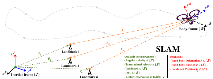
Figure 1: SLAM estimation problem.

III-A SLAM Kinematics and Measurements

Let $X=\left(\boldsymbol{T},\overline{{\rm p}}\right)\in\mathbb{SLAM}_{n}\left(3\right)$ denote the true configuration of the SLAM problem with $\boldsymbol{T}\in\mathbb{SE}\left(3\right)$ as in (1) and $\overline{{\rm p}}=\left[\overline{{\rm p}}_{1},\overline{{\rm p}}_{2},\ldots,\overline{{\rm p}}_{n}\right]\in\overline{\mathcal{M}}^{n}$. Notice that $X$ is unknown. A group of measurements is available in $\left\{\mathcal{B}\right\}$ and can be employed for SLAM estimation, namely 1) body-frame measurements associated with attitude determination, 2) landmark measurements, and 3) group velocity measurements. Assume that there are $n_{R}$ body-frame vectors suitable for attitude determination and available for measurement defined by [18, 19]

$$\overset{\circ}{a}_{j}=\boldsymbol{T}^{-1}\overset{\circ}{r}_{j}+\overset{\circ}{b}_{j}^{a}+\overset{\circ}{n}_{j}^{a}\in\overset{\circ}{\mathcal{M}},\hskip 10.00002ptj=1,2,\ldots,n_{R}$$

or equivalently

$$a_{j}=R^{\top}r_{j}+b_{j}^{a}+n_{j}^{a}\in\mathbb{R}^{3}$$ (16)

where $r_{j}$ denotes known inertial-frame vector, $b_{j}^{a}$ denotes unknown constant bias, and $n_{j}^{a}$ stands for unknown random noise of the $j$th measurement. Note that the inverse of $\boldsymbol{T}$ is $\boldsymbol{T}^{-1}=\left[\begin{array}[]{cc}R^{\top}&-R^{\top}P\\ \underline{\mathbf{0}}_{3}^{\top}&1\end{array}\right]\in\mathbb{SE}\left(3\right)$. The measurements in (16) exemplify a low cost IMU. It is a common practice to normalize $r_{j}$ and $a_{j}$ in (16) as follows

$$\upsilon_{j}^{r}=\frac{r_{j}}{\left\|r_{j}\right\|},\hskip 10.00002pt\upsilon_{j}^{a}=\frac{a_{j}}{\left\|a_{j}\right\|}$$ (17)

The normalized values in (17) will be part of the subsequent estimation. Consider combining the normalized vectors into two distinct sets as follows

$$\begin{cases}\upsilon^{r}&=\left[\upsilon_{1}^{r},\upsilon_{2}^{r},\ldots,\upsilon_{n_{R}}^{r}\right]\in\left\{\mathcal{I}\right\}\\ \upsilon^{a}&=\left[\upsilon_{1}^{a},\upsilon_{2}^{a},\ldots,\upsilon_{n_{R}}^{a}\right]\in\left\{\mathcal{B}\right\}\end{cases}$$ (18)

Remark 1.

Rigid-body’s attitude can be established provided that at least three non-collinear vectors in $\left\{\mathcal{B}\right\}$ along with their observations in $\left\{\mathcal{I}\right\}$ are obtainable at each time sample. In case of $n_{R}=2$, the third measurement in $\left\{\mathcal{B}\right\}$ and its observation in $\left\{\mathcal{I}\right\}$ is to be calculated via the cross product $\upsilon_{3}^{a}=\upsilon_{1}^{a}\times\upsilon_{2}^{a}$ and $\upsilon_{3}^{r}=\upsilon_{1}^{r}\times\upsilon_{2}^{r}$, respectively ensuring that the two sets in (17) are with rank 3.

Assume that $n$ landmarks are available for measurement in the body-frame via, for example, low-cost inertial vision units. The $i$th measurement is as follows [22, 2]:

$$\overline{y}_{i}=\boldsymbol{T}^{-1}\overline{{\rm p}}_{i}+\overset{\circ}{b}_{i}^{y}+\overset{\circ}{n}_{i}^{y}\in\overline{\mathcal{M}},\hskip 10.00002pt\forall i=1,2,\ldots,n$$

or equivalently

$$y_{i}=R^{\top}\left({\rm p}_{i}-P\right)+b_{i}^{y}+n_{i}^{y}\in\mathbb{R}^{3}$$ (19)

with $R$, $P$, and ${\rm p}_{i}$ representing the true attitude and position of the robot, and landmark position, respectively, while $b_{i}^{y}$ and $n_{i}^{y}$ stand for unknown constant bias and random noise, respectively, for all $y_{i},b_{i}^{y},n_{i}^{y}\in\left\{\mathcal{B}\right\}$.

Assumption 1.

A minimum of three landmarks available for measurement is necessary to define a plane $\overline{y}=\left[\overline{y}_{1},\overline{y}_{2},\ldots,\overline{y}_{n}\right]\in\overline{\mathcal{M}}^{n}$.

Consider $\mathcal{Y}=\left(\left[U\right]_{\wedge},\overset{\circ}{{\rm v}}\right)\in\mathfrak{slam}_{n}\left(3\right)$ to be the true group velocity which is bounded and continuous with $\overset{\circ}{{\rm v}}=\left[\overset{\circ}{{\rm v}}_{1},\overset{\circ}{{\rm v}}_{2},\ldots,\overset{\circ}{{\rm v}}_{n}\right]\in\overset{\circ}{\mathcal{M}}^{n}$. Note that $\mathcal{Y}$ is given through sensor measurements. Hence, the true motion dynamics of the vehicle’s pose and $n$-landmarks are

$$\begin{cases}\dot{\boldsymbol{T}}&=\boldsymbol{T}\left[U\right]_{\wedge}\\ \dot{{\rm p}}_{i}&=R{\rm v}_{i},\hskip 10.00002pt\forall i=1,2,\ldots,n\end{cases}$$ (20)

The dynamics in (20) can be expressed as

$$\begin{cases}\dot{R}&=R\left[\Omega\right]_{\times}\\ \dot{P}&=RV\\ \dot{{\rm p}}_{i}&=R{\rm v}_{i},\hskip 10.00002pt\forall i=1,2,\ldots,n\end{cases}$$

with $U=\left[\Omega^{\top},V^{\top}\right]^{\top}\in\mathbb{R}^{6}$ referring to the group velocity vector of the rigid-body where $\Omega\in\mathbb{R}^{3}$ is the true angular velocity and $V\in\mathbb{R}^{3}$ is the true translational velocity. ${\rm v}_{i}\in\mathbb{R}^{3}$ defines the $i$th linear velocity of the landmark in the moving-frame for all $\Omega,V,{\rm v}_{i}\in\left\{\mathcal{B}\right\}$. The measurements of angular and translational velocity are defined as

$$\begin{cases}\Omega_{m}&=\Omega+b_{\Omega}+n_{\Omega}\in\mathbb{R}^{3}\\ V_{m}&=V+b_{V}+n_{V}\in\mathbb{R}^{3}\end{cases}$$ (21)

where $b_{\Omega}$ and $b_{V}$ denote unknown constant bias, and $n_{\Omega}$ and $n_{V}$ denote unknown random noise. Define the group of velocity measurements, bias, and noise as $U_{m}=\left[\Omega_{m}^{\top},V_{m}^{\top}\right]^{\top}$, $b_{U}=\left[b_{\Omega}^{\top},b_{V}^{\top}\right]^{\top}$, and $n_{U}=\left[n_{\Omega}^{\top},n_{V}^{\top}\right]^{\top}$, respectively, for all $U_{m},b_{U},n_{U}\in\mathbb{R}^{6}$. This work concerns exclusively fixed landmark environments, thereby $\dot{{\rm p}}_{i}=\underline{\mathbf{0}}_{3}$ and ${\rm v}_{i}=\underline{\mathbf{0}}_{3}$ $\forall i=1,2,\ldots,n$.

III-B SLAM Kinematics in Stochastic Sense

Recall the expression of group velocity measurements in (21). Since derivative of a Gaussian process results a Gaussian process, the SLAM dynamics in (20) can be rewritten with respect to Brownian motion process vector $d\beta_{U}/dt\in\mathbb{R}^{6}$ [28, 29]. Assume $\left\{n_{U},t\geq t_{0}\right\}$ to be a vector representation of the independent Brownian motion process

$$n_{U}=\mathcal{Q}_{U}\frac{d\beta_{U}}{dt}\in\mathbb{R}^{6}$$ (22)

where $\mathcal{Q}_{U}\in\mathbb{R}^{6\times 6}$ denotes an unknown nonzero nonnegative time-variant diagonal matrix whose elements are bounded. The related covariance of the noise $n_{U}$ can be expressed as $\mathcal{Q}_{U}^{2}=\mathcal{Q}_{U}\mathcal{Q}_{U}^{\top}$. The following properties characterize the Brownian motion process [30, 29, 31, 22, 32]:

$$\mathbb{P}\left\{\beta_{U}\left(0\right)=0\right\}=1,\hskip 10.00002pt\mathbb{E}\left[d\beta_{U}/dt\right]=0,\hskip 10.00002pt\mathbb{E}\left[\beta_{U}\right]=0$$

In view of (20), (21), and (22), SLAM dynamics could be represented by a stochastic differential equation

$$\begin{cases}d\boldsymbol{T}&=\boldsymbol{T}\left[U_{m}-b_{U}\right]_{\wedge}dt-\boldsymbol{T}\left[\mathcal{Q}_{U}d\beta_{U}\right]_{\wedge}\\ d{\rm p}_{i}&=R{\rm v}_{i}dt,\hskip 10.00002pt\forall i=1,2,\ldots,n\end{cases}$$ (23)

Or equivalently

$$\begin{cases}dR&=R\left[\Omega_{m}-b_{\Omega}\right]_{\times}dt-R\left[\mathcal{Q}_{\Omega}d\beta_{\Omega}\right]_{\times}\\ dP&=R\left(V_{m}-b_{V}\right)dt-R\mathcal{Q}_{V}d\beta_{V}\\ d{\rm p}_{i}&=R{\rm v}_{i}dt,\hskip 10.00002pt\forall i=1,2,\ldots,n\end{cases}$$

where $U=U_{m}-b_{U}-n_{U}$ is considered. Given unknown bias $b_{U}$ and unknown time-variant covariance matrix $\mathcal{Q}_{U}$, with the aim of achieving adaptive stabilization, define $\sigma$ as the upper bound of $\mathcal{Q}_{U}^{2}$

$$\sigma=\left[\begin{array}[]{c}{\rm max}\left\{\mathcal{Q}_{\Omega\left(1,1\right)}^{2},\mathcal{Q}_{V\left(1,1\right)}^{2}\right\}\\ {\rm max}\left\{\mathcal{Q}_{\Omega\left(2,2\right)}^{2},\mathcal{Q}_{V\left(2,2\right)}^{2}\right\}\\ {\rm max}\left\{\mathcal{Q}_{\Omega\left(3,3\right)}^{2},\mathcal{Q}_{V\left(3,3\right)}^{2}\right\}\end{array}\right]\in\mathbb{R}^{3}$$ (24)

with ${\rm max}\left\{\cdot\right\}$ being maximum value of the corresponding elements.

Assumption 2.

(Uniform boundedness of $b_{U}$ and $\sigma$) Consider $b_{U}$ and $\sigma$ to belong to a known compact set $\varLambda_{U}$ with $b_{U},\sigma\in\varLambda_{U}\subset\mathbb{R}^{3}$, such that $b_{U}$ and $\sigma$ are upper bounded by a constant $\varPi$ where $||\varLambda_{U}||\leq\overline{\varLambda}<\infty$.

III-C Error Criteria

Define the pose estimate as

$$\hat{\boldsymbol{T}}=\left[\begin{array}[]{cc}\hat{R}&\hat{P}\\ \underline{\mathbf{0}}_{3}^{\top}&1\end{array}\right]\in\mathbb{SE}\left(3\right)$$

with $\hat{R}$ being the estimate of $R$, and $\hat{P}$ being the estimate of $P$ in (1). Define $\overline{\hat{y}}_{i}=\hat{\boldsymbol{T}}^{-1}\overline{\hat{{\rm p}}}_{i}$ where $\hat{{\rm p}}_{i}$ is the $i$th landmark estimate of ${\rm p}_{i}$. Let the pose error (true relative to estimated) be

$$\tilde{\boldsymbol{T}}=\hat{\boldsymbol{T}}\boldsymbol{T}^{-1} =\left[\begin{array}[]{cc}\hat{R}&\hat{P}\\ \underline{\mathbf{0}}_{3}^{\top}&1\end{array}\right]\left[\begin{array}[]{cc}R^{\top}&-R^{\top}P\\ \underline{\mathbf{0}}_{3}^{\top}&1\end{array}\right]$$ (29)

$$=\left[\begin{array}[]{cc}\tilde{R}&\tilde{P}\\ \underline{\mathbf{0}}_{3}^{\top}&1\end{array}\right]$$ (32)

with $\tilde{R}=\hat{R}R^{\top}$ being the error in orientation and $\tilde{P}=\hat{P}-\tilde{R}P$ being the error in position of the rigid-body. Pose estimation aims to asymptotically drive $\tilde{\boldsymbol{T}}\rightarrow\mathbf{I}_{4}$ in order to achieve this goal $\tilde{R}\rightarrow\mathbf{I}_{3}$ and $\tilde{P}\rightarrow\underline{\mathbf{0}}_{3}$. Let the landmark position error (true relative to estimated) be

$$\overset{\circ}{e}_{i}=\overline{\hat{{\rm p}}}_{i}-\tilde{\boldsymbol{T}}\,\overline{{\rm p}}_{i},\hskip 10.00002pt\forall i=1,2,\ldots,n$$ (33)

such that $\overset{\circ}{e}_{i}=\left[e_{i}^{\top},0\right]^{\top}\in\overset{\circ}{\mathcal{M}}$ and $\overline{\hat{{\rm p}}}_{i}=\left[\hat{{\rm p}}_{i}^{\top},1\right]^{\top}\in\overline{\mathcal{M}}$. Note that $\overset{\circ}{e}_{i}=\overline{\hat{{\rm p}}}_{i}-\hat{\boldsymbol{T}}\boldsymbol{T}^{-1}\,\overline{{\rm p}}_{i}$, and therefore from (19) one has

$$\overset{\circ}{e}_{i}=\overline{\hat{{\rm p}}}_{i}-\hat{\boldsymbol{T}}\,\overline{y}_{i},\hskip 10.00002pt\forall i=1,2,\ldots,n$$ (34)

which leads to

$$\overset{\circ}{e}_{i} =\left[\begin{array}[]{c}\hat{{\rm p}}_{i}\\ 1\end{array}\right]-\left[\begin{array}[]{cc}\hat{R}&\hat{P}\\ \underline{\mathbf{0}}_{3}^{\top}&1\end{array}\right]\left[\begin{array}[]{c}R^{\top}\left({\rm p}_{i}-P\right)\\ 1\end{array}\right]$$ (41)

$$=\left[\begin{array}[]{c}\tilde{{\rm p}}_{i}-\tilde{P}\\ 0\end{array}\right]\in\overset{\circ}{\mathcal{M}}$$ (44)

with $\tilde{{\rm p}}_{i}=\hat{{\rm p}}_{i}-\tilde{R}{\rm p}_{i}$ and $\tilde{P}=\hat{P}-\tilde{R}P$. Considering the fact that the last row of the matrix in (44) is a zero, define the stochastic differential equation of the error above as

$$de_{i}= \mathcal{F}_{i}dt+\mathcal{G}_{i}\mathcal{Q}_{U}d\beta_{U},\hskip 10.00002pt\forall i=1,2,\ldots,n$$ (45)

where the stochastic dynamics in (45) are to be obtained in the stochastic filter. Taking in consideration the group velocity in (21) with $\hat{b}_{U}=\left[\hat{b}_{\Omega}^{\top},\hat{b}_{V}^{\top}\right]^{\top}$ being the unknown bias estimate of $b_{U}$, define the bias error as

$$\begin{cases}\tilde{b}_{\Omega}&=b_{\Omega}-\hat{b}_{\Omega}\\ \tilde{b}_{V}&=b_{V}-\hat{b}_{V}\end{cases}$$ (46)

where $\tilde{b}_{U}=b_{U}-\hat{b}_{U}=\left[\tilde{b}_{\Omega}^{\top},\tilde{b}_{V}^{\top}\right]^{\top}\in\mathbb{R}^{6}$. Also, consider $\hat{\sigma}$ to be the estimate of $\sigma$ in (24). Define the error between $\hat{\sigma}$ and $\sigma$ as follows

$$\tilde{\sigma}=\sigma-\hat{\sigma}$$ (47)

The subsequent Definitions and Lemmas are applicable in the derivation process of the nonlinear stochastic estimator for SLAM.

Definition 1.

Let $\mathcal{U}_{s}$ be a non-attractive forward invariant unstable subset of $\mathbb{SO}\left(3\right)$

$$\mathcal{U}_{s}=\left\{\left.\tilde{R}\left(0\right)\in\mathbb{SO}\left(3\right)\right|{\rm Tr}\{\tilde{R}(0)\}=-1\right\}$$ (48)

The only three possible scenarios for $\tilde{R}\left(0\right)\in\mathcal{U}_{s}$ are: $\tilde{R}\left(0\right)={\rm diag}(1,-1,-1)$, $\tilde{R}\left(0\right)={\rm diag}(-1,1,-1)$, and $\tilde{R}\left(0\right)={\rm diag}(-1,-1,1)$.

Lemma 1.

Define $\tilde{R}\in\mathbb{SO}\left(3\right)$, $M=M^{\top}\in\mathbb{R}^{3\times 3}$ such that ${\rm rank}\left\{M\right\}=3$ and ${\rm Tr}\left\{M\right\}=3$. Define $\breve{\mathbf{M}}={\rm Tr}\left\{M\right\}\mathbf{I}_{3}-M$ with $\underline{\lambda}=\underline{\lambda}(\breve{\mathbf{M}})$ being the minimum singular value of $\breve{\mathbf{M}}$. Thereby, the following holds:

$$||\tilde{R}M||_{{\rm I}} \leq\frac{2}{\underline{\lambda}}\frac{||\mathbf{vex}\left(\boldsymbol{\mathcal{P}}_{a}(\tilde{R}M)\right)||^{2}}{1+{\rm Tr}\{\tilde{R}MM^{-1}\}}$$ (49)

Proof. See Lemma 1 [19].

Definition 2.

Consider the stochastic differential system in (45), and let $\boldsymbol{{\rm V}}\left(e_{1},\ldots,e_{n}\right)$ be a twice differentiable function $\boldsymbol{{\rm V}}\left(e_{1},\ldots,e_{n}\right)\in\mathcal{C}^{2}$. The differential operator $\mathcal{L}\boldsymbol{{\rm V}}\left(e_{1},\ldots,e_{n}\right)$ is expressed as below

$$\mathcal{L}\boldsymbol{{\rm V}}\left(e_{1},\ldots,e_{n}\right)=\sum_{i=1}^{n}\left(\boldsymbol{{\rm V}}_{e_{i}}^{\top}\mathcal{F}_{i}+\frac{1}{2}{\rm Tr}\left\{\mathcal{G}_{i}\mathcal{Q}_{U}^{2}\mathcal{G}_{i}^{\top}\boldsymbol{{\rm V}}_{e_{i}e_{i}}\right\}\right)$$

such that $\boldsymbol{{\rm V}}_{e_{i}}=\partial\boldsymbol{{\rm V}}/\partial e_{i}$, and $\boldsymbol{{\rm V}}_{e_{i}e_{i}}=\partial^{2}\boldsymbol{{\rm V}}/\partial e_{i}^{2}$ $\forall i=1,2,\ldots,n$.

Definition 3.

[18, 22, 33] Consider the stochastic differential system in (45) with trajectory $e_{i}$ being SGUUB if for a given compact set $\Sigma\in\mathbb{R}^{4}$ and any $e_{i}\left(t_{0}\right)$, there exists a positive constant $\kappa>0$, and a time constant $\tau=\tau\left(\kappa,e_{i}\left(t_{0}\right)\right)$ with $\mathbb{E}\left[\left\|e_{i}\left(t_{0}\right)\right\|\right]<\kappa,\forall t>t_{0}+\tau$.

Lemma 2.

[31] Consider the stochastic dynamics in (45) to be assigned with a potential function $\boldsymbol{{\rm V}}\in\mathcal{C}^{2}$ where $\boldsymbol{{\rm V}}:\mathbb{R}^{3}\rightarrow\mathbb{R}_{+}$. Suppose there exist class $\mathcal{K}_{\infty}$ functions $\bar{\alpha}_{1}\left(\cdot\right)$ and $\bar{\alpha}_{2}\left(\cdot\right)$, constants $\eta_{1}>0$ and $\eta_{2}\geq 0$ such that

$$\bar{\alpha}_{1}\left(e_{1},\ldots,e_{n}\right)\leq\boldsymbol{{\rm V}}\left(e_{1},\ldots,e_{n}\right)\leq\bar{\alpha}_{2}\left(e_{1},\ldots,e_{n}\right)$$ (50)

$$\mathcal{L}\boldsymbol{{\rm V}}\left(e_{1},\ldots,e_{n}\right)= \sum_{i=1}^{n}\left(\boldsymbol{{\rm V}}_{e_{i}}^{\top}\mathcal{F}_{i}+\frac{1}{2}{\rm Tr}\left\{\mathcal{G}_{i}\mathcal{Q}_{U}^{2}\mathcal{G}_{i}^{\top}\boldsymbol{{\rm V}}_{e_{i}e_{i}}\right\}\right)$$

$$\leq -\eta_{1}\boldsymbol{{\rm V}}\left(e_{1},\ldots,e_{n}\right)+\eta_{2}$$ (51)

then for $e_{i}\in\mathbb{R}^{4}$, there is almost a unique strong solution on $\left[0,\infty\right)$ for the stochastic dynamics in (45). Moreover, the solution $e_{i}$ is bounded in probability where

$$\mathbb{E}\left[\boldsymbol{{\rm V}}\left(e_{1},\ldots,e_{n}\right)\right]\leq\boldsymbol{{\rm V}}\left(e_{1}\left(0\right),\ldots,e_{n}\left(0\right)\right){\rm exp}\left(-\eta_{1}t\right)+\frac{\eta_{2}}{\eta_{1}}$$ (52)

In addition, if the inequality in (52) is met, $e_{i}$ in (45) is SGUUB in the mean square.

The existence of a unique solution and proof of Lemma 2 can be found in [31].

Lemma 3.

(Young’s inequality) Let $a\in\mathbb{R}^{n}$ and $b\in\mathbb{R}^{n}$. Define $c_{1}>1$ and $c_{2}>1$ such that $\left(c_{1}-1\right)\left(c_{2}-1\right)=1$, and $\varrho>0$ as a small constant. Consequently, the following holds:

$$a^{\top}b \leq\left(1/c_{1}\right)\varrho^{c_{1}}\left\|a\right\|^{c_{1}}+\left(1/c_{2}\right)\varrho^{-c_{2}}\left\|b\right\|^{c_{2}}$$ (53)

Prior to moving forward, it is important to recall that the true SLAM dynamics in (20) 1) are nonlinear and 2) are posed on the Lie group of $\mathbb{SLAM}_{n}\left(3\right)=\mathbb{SE}\left(3\right)\times\overline{\mathcal{M}}^{n}$ where $X=\left(\boldsymbol{T},\overline{{\rm p}}\right)\in\mathbb{SLAM}_{n}\left(3\right)$. Additionally, the tangent space of $\mathbb{SLAM}_{n}\left(3\right)$ is $\mathfrak{slam}_{n}\left(3\right)=\mathfrak{se}\left(3\right)\times\overset{\circ}{\mathcal{M}}^{n}$ such that and $\mathcal{Y}=\left(\left[U\right]_{\wedge},\overset{\circ}{{\rm v}}\right)\in\mathfrak{slam}_{n}\left(3\right)$. With the aim of proposing a robust stochastic filter able to produce good results, the proposed filter design should imitate the true nonlinearity of the SLAM problem and should be modeled on the Lie group of $\mathbb{SLAM}_{n}\left(3\right)$ with the tangent space $\mathfrak{slam}_{n}\left(3\right)$. Complying with the above-mentioned requirements, the structure of the stochastic filter is $\hat{X}=\left(\hat{\boldsymbol{T}},\overline{\hat{{\rm p}}}\right)\in\mathbb{SLAM}_{n}\left(3\right)$ and $\hat{\mathcal{Y}}=\left([\hat{U}]_{\wedge},\overset{\circ}{\hat{{\rm v}}}\right)\in\mathfrak{slam}_{n}\left(3\right)$ with $\hat{\boldsymbol{T}}\in\mathbb{SE}\left(3\right)$ and $\overline{\hat{{\rm p}}}=\left[\overline{\hat{{\rm p}}}_{1},\ldots,\overline{\hat{{\rm p}}}_{n}\right]\in\overline{\mathcal{M}}^{n}$ being pose estimates and landmark positions, respectively, and $\hat{U}\in\mathfrak{se}\left(3\right)$ and $\overset{\circ}{\hat{{\rm v}}}=\left[\overset{\circ}{\hat{{\rm v}}}_{1},\ldots,\overset{\circ}{\hat{{\rm v}}}_{n}\right]\in\overset{\circ}{\mathcal{M}}^{n}$ being velocities to be designed in the following Section. It is worth noting that $\overset{\circ}{\hat{{\rm v}}}_{i}=\left[\hat{{\rm v}}_{i}^{\top},0\right]\in\overset{\circ}{\mathcal{M}}$ and $\overline{\hat{{\rm p}}}_{i}=\left[\hat{{\rm p}}_{i}^{\top},1\right]^{\top}\in\overline{\mathcal{M}}$ for all $i=1,2,\ldots,n$ and $\hat{{\rm v}}_{i},\hat{{\rm p}}_{i}\in\mathbb{R}^{3}$.

IV Nonlinear Stochastic Filter Design

The SLAM nonlinear stochastic filter design is proposed in this Section. With the aim of defining the concept of the nonlinear SLAM filtering and paving the way for the novel nonlinear stochastic filter solution presented in the second subsection, the first subsection introduces a nonlinear deterministic filter that operates based only on the surrounding landmark measurements which is similar in the structure to [7, 8]. In contrast to the deterministic filter, the novel nonlinear stochastic SLAM filter relies on measurements collected by a low-cost IMU and measurements of the landmarks. The first simple filter will provide a benchmark for the proposed stochastic solution.

IV-A Nonlinear Deterministic Filter Design without IMU

Consider the nonlinear filter design for SLAM:

$$\dot{\hat{\boldsymbol{T}}} =\hat{\boldsymbol{T}}\left[U_{m}-\hat{b}_{U}-W_{U}\right]_{\wedge}$$ (54)

$$\dot{{\rm\hat{p}}}_{i} =-k_{p}e_{i},\hskip 10.00002pti=1,2,\ldots,n$$ (55)

$$\dot{\hat{b}}_{U} =-\sum_{i=1}^{n}\frac{\Gamma}{\alpha_{i}}\left[\begin{array}[]{c}\left[y_{i}\right]_{\times}\hat{R}^{\top}\\ \hat{R}^{\top}\end{array}\right]e_{i}$$ (58)

$$W_{U} =-\sum_{i=1}^{n}\frac{k_{w}}{\alpha_{i}}\left[\begin{array}[]{c}\left[y_{i}\right]_{\times}\hat{R}^{\top}\\ \hat{R}^{\top}\end{array}\right]e_{i}$$ (61)

with $k_{w}$, $k_{p}$, $\Gamma$, and $\alpha_{i}$ being positive constants, $e_{i}$ being as given in (34) for all $i=1,2,\cdots,n$, $W_{U}=\left[W_{\Omega}^{\top},W_{V}^{\top}\right]^{\top}\in\mathbb{R}^{6}$ being a correction factor, and $\hat{b}_{U}=\left[\hat{b}_{\Omega}^{\top},\hat{b}_{V}^{\top}\right]^{\top}\in\mathbb{R}^{6}$ being the estimate of $b_{U}$.

Theorem 1.

Consider the true motion of SLAM dynamics to be $\dot{X}=\left(\dot{\boldsymbol{T}},\dot{\overline{{\rm p}}}\right)$ as in (20), the output to be landmark measurements ($\overline{y}_{i}=\boldsymbol{T}^{-1}\overline{{\rm p}}_{i}$) for all $i=1,2,\ldots,n$ and the velocity measurements in (20) to be attached only with constant bias where $U_{m}=U+b_{U}$ and $n_{U}=0$. Let Assumption 1 hold true and the deterministic filter be as in (54), (55), (58), and (61) combined with the measurements of $U_{m}$ and $\overline{y}_{i}$. Set the design parameters $k_{w}$, $k_{p}$, $\Gamma$, and $\alpha_{i}$ as positive scalars for all $i=1,2,\ldots,n$. Also, consider the set

$$\mathcal{S}= \left\{\left(e_{1},e_{2},\ldots,e_{n}\right)\in\mathbb{R}^{3}\times\mathbb{R}^{3}\times\cdots\times\mathbb{R}^{3}\right|$$

$$\hskip 90.00014pte_{i}=\underline{\mathbf{0}}_{3}\forall i=1,2,\ldots n\}$$ (62)

Then 1) the error $e_{i}$ in (33) is exponentially regulated to the set $\mathcal{S}$, 2) $\tilde{\boldsymbol{T}}$ remains bounded and 3) given constants $R_{c}\in\mathbb{SO}\left(3\right)$ and $P_{c}\in\mathbb{R}^{3}$ one has $\tilde{R}\rightarrow R_{c}$ and $\tilde{P}\rightarrow P_{c}$ as $t\rightarrow\infty$.

Proof.

Since $\boldsymbol{\dot{T}}^{-1}=-\boldsymbol{T}^{-1}\boldsymbol{\dot{T}}\boldsymbol{T}^{-1}$, one obtains the error dynamics of $\tilde{\boldsymbol{T}}$ defined in (32) as follows

$$\dot{\tilde{\boldsymbol{T}}} =\dot{\hat{\boldsymbol{T}}}\boldsymbol{T}^{-1}+\hat{\boldsymbol{T}}\dot{\boldsymbol{T}}^{-1}$$

$$=\hat{\boldsymbol{T}}\left[U+\tilde{b}_{U}-W_{U}\right]_{\wedge}\boldsymbol{T}^{-1}-\hat{\boldsymbol{T}}\left[U\right]_{\wedge}\boldsymbol{T}^{-1}$$

$$=\hat{\boldsymbol{T}}\left[\tilde{b}_{U}-W_{U}\right]_{\wedge}\hat{\boldsymbol{T}}^{-1}\tilde{\boldsymbol{T}}$$ (63)

Thereby, the error dynamics of $\overset{\circ}{e}_{i}$ in (33) are

$$\overset{\circ}{\dot{e}}_{i} =\overset{\circ}{\dot{\hat{{\rm p}}}}_{i}-\dot{\tilde{\boldsymbol{T}}}\,\overline{{\rm p}}_{i}-\tilde{\boldsymbol{T}}\,\dot{\overline{{\rm p}}}_{i}$$

$$=\overset{\circ}{\dot{\hat{{\rm p}}}}_{i}-\hat{\boldsymbol{T}}\left[\tilde{b}_{U}-W_{U}\right]_{\wedge}\hat{\boldsymbol{T}}^{-1}\tilde{\boldsymbol{T}}\,\overline{{\rm p}}_{i}$$ (64)

From (63), one finds

$$\hat{\boldsymbol{T}}\left[\tilde{b}_{U}\right]_{\wedge}\hat{\boldsymbol{T}}^{-1} =\left[\begin{array}[]{cc}\hat{R}&\hat{P}\\ \underline{\mathbf{0}}_{3}^{\top}&1\end{array}\right]\left[\begin{array}[]{cc}\left[\tilde{b}_{\Omega}\right]_{\times}&\tilde{b}_{V}\\ \underline{\mathbf{0}}&0\end{array}\right]\left[\begin{array}[]{cc}\hat{R}^{\top}&-\hat{R}^{\top}\hat{P}\\ \underline{\mathbf{0}}_{3}^{\top}&1\end{array}\right]$$ (71)

$$=\left[\begin{array}[]{cc}\hat{R}\left[\tilde{b}_{\Omega}\right]_{\times}\hat{R}^{\top}&\hat{R}\tilde{b}_{V}-\hat{R}\left[\tilde{b}_{\Omega}\right]_{\times}\hat{R}^{\top}\hat{P}\\ \underline{\mathbf{0}}_{3}^{\top}&0\end{array}\right]$$ (74)

$$=\left[\begin{array}[]{c}\hat{R}\tilde{b}_{\Omega}\\ \hat{R}\tilde{b}_{V}+\left[\hat{P}\right]_{\times}\hat{R}\tilde{b}_{\Omega}\end{array}\right]_{\wedge}\in\mathfrak{se}\left(3\right)$$ (77)

where $\left[R\tilde{b}_{\Omega}\right]_{\times}=R\left[\tilde{b}_{\Omega}\right]_{\times}R^{\top}$ as defined in (10). Recalling the definition of wedge operator in (3), one finds that (77) becomes

$$\hat{\boldsymbol{T}}\left[\tilde{b}_{U}\right]_{\wedge}\hat{\boldsymbol{T}}^{-1}=\left[\left[\begin{array}[]{cc}\hat{R}&0_{3\times 3}\\ \left[\hat{P}\right]_{\times}\hat{R}&\hat{R}\end{array}\right]\tilde{b}_{U}\right]_{\wedge}$$ (78)

According to (78) and (64), one has

$$\hat{\boldsymbol{T}}\left[\tilde{b}_{U}\right]_{\wedge}\hat{\boldsymbol{T}}^{-1}\tilde{\boldsymbol{T}}\,\overline{{\rm p}}_{i} =\left[\left[\begin{array}[]{cc}\hat{R}&0_{3\times 3}\\ \left[\hat{P}\right]_{\times}\hat{R}&\hat{R}\end{array}\right]\tilde{b}_{U}\right]_{\wedge}\left[\begin{array}[]{c}\hat{R}y_{i}+\hat{P}\\ 1\end{array}\right]$$ (83)

$$=\left[\begin{array}[]{c}-\left[\hat{R}y_{i}\right]_{\times}\hat{R}\tilde{b}_{\Omega}+\hat{R}\tilde{b}_{V}\\ 0\end{array}\right]$$ (86)

$$=\left[\begin{array}[]{cc}-\hat{R}\left[y_{i}\right]_{\times}&\hat{R}\\ \underline{\mathbf{0}}_{3}^{\top}&\underline{\mathbf{0}}_{3}^{\top}\end{array}\right]\tilde{b}_{U}$$ (89)

In view of (64) and (89), one can rewrite (64) as

$$\overset{\circ}{\dot{e}}_{i} =\overset{\circ}{\dot{\hat{{\rm p}}}}_{i}-\left[\begin{array}[]{cc}-\hat{R}\left[y_{i}\right]_{\times}&\hat{R}\\ \underline{\mathbf{0}}_{3}^{\top}&\underline{\mathbf{0}}_{3}^{\top}\end{array}\right]\left(\tilde{b}_{U}-W_{U}\right)$$ (92)

The last row in (92) are zeros, thereby, one obtains

$$\dot{e}_{i} =\dot{\hat{{\rm p}}}_{i}-\left[\begin{array}[]{cc}-\hat{R}\left[y_{i}\right]_{\times}&\hat{R}\end{array}\right]\left(\tilde{b}_{U}-W_{U}\right)$$ (94)

Consider the candidate Lyapunov function $\boldsymbol{{\rm V}}=\boldsymbol{{\rm V}}\left(e_{1},\ldots,e_{n},\tilde{b}_{U}\right)$

$$\boldsymbol{{\rm V}}=\sum_{i=1}^{n}\frac{1}{2\alpha_{i}}e_{i}^{\top}e_{i}+\frac{1}{2}\tilde{b}_{U}^{\top}\Gamma^{-1}\tilde{b}_{U}$$ (95)

The time derivative of (95) is

$$\dot{\boldsymbol{{\rm V}}}= \sum_{i=1}^{n}\frac{1}{\alpha_{i}}e_{i}^{\top}\dot{e}_{i}-\tilde{b}_{U}^{\top}\Gamma^{-1}\dot{\hat{b}}_{U}$$

$$= \sum_{i=1}^{n}\frac{1}{\alpha_{i}}e_{i}^{\top}\dot{\hat{{\rm p}}}_{i}-\sum_{i=1}^{n}\frac{1}{\alpha_{i}}e_{i}^{\top}\left[\begin{array}[]{cc}-\hat{R}\left[y_{i}\right]_{\times}&\hat{R}\end{array}\right]\left(\tilde{b}_{U}-W_{U}\right)$$ (97)

$$-\tilde{b}_{U}^{\top}\Gamma^{-1}\dot{\hat{b}}_{U}$$ (98)

Replacing $W_{U}$, $\dot{\hat{b}}_{U}$ and $\dot{\hat{{\rm p}}}_{i}$ with their expressions in (55), (58) and (61), respectively, one obtains

$$\dot{\boldsymbol{{\rm V}}}= -\sum_{i=1}^{n}\frac{k_{p}}{\alpha_{i}}\left\|e_{i}\right\|^{2}-k_{w}\left\|\sum_{i=1}^{n}\frac{e_{i}}{\alpha_{i}}\right\|^{2}$$

$$-k_{w}\left\|\sum_{i=1}^{n}\left[y_{i}\right]_{\times}\hat{R}^{\top}\frac{e_{i}}{\alpha_{i}}\right\|^{2}$$ (99)

Based on (99) the time derivative of $\boldsymbol{{\rm V}}$ is negative definite where $\dot{\boldsymbol{{\rm V}}}$ equals to zero at $e_{i}=\underline{\mathbf{0}}_{3}$. The result in (99) affirms that $e_{i}$ is exponentially regulated to the set $\mathcal{S}$ given in (62). Based on Barbalat Lemma, $\dot{\boldsymbol{{\rm V}}}$ is negative, continuous and approaches the origin implying that $\tilde{\boldsymbol{T}}$, $\tilde{b}_{U}$, and $\ddot{e}_{i}$ stay bounded. Also, the expression in (44) demonstrates that if $e_{i}\rightarrow\underline{\mathbf{0}}_{3}$, then $\tilde{{\rm p}}_{i}-\tilde{P}\rightarrow\underline{\mathbf{0}}_{3}$, and accordingly by (33) one has $\overline{\hat{{\rm p}}}_{i}-\tilde{\boldsymbol{T}}\,\overline{{\rm p}}_{i}\rightarrow\underline{\mathbf{0}}_{4}$. As such, $\tilde{\boldsymbol{T}}$ is upper bounded with $\tilde{R}\rightarrow R_{c}$ and $\tilde{P}\rightarrow P_{c}$ as $t\rightarrow\infty$ which completes the proof.∎

IV-B Nonlinear Stochastic Filter Design with IMU

The nonlinear deterministic filter design in Subsection IV-A allows $e_{i}=\tilde{{\rm p}}_{i}-\tilde{P}\rightarrow\underline{\mathbf{0}}_{3}$ exponentially where $\tilde{P}=\hat{P}-\tilde{R}P$ and $\tilde{{\rm p}}_{i}=\hat{{\rm p}}_{i}-\tilde{R}{\rm p}_{i}$. However, $\tilde{R}\rightarrow R_{c}$ and $\tilde{P}\rightarrow P_{c}$ as $t\rightarrow\infty$ such that $R_{c}\in\mathbb{SO}\left(3\right)$ and $P_{c}\in\mathbb{R}^{3}$ are constants. Hence, for the case when $R\left(0\right)$ and $P\left(0\right)$ are not precisely known, the error in $\tilde{R}$, $\tilde{P}$, and $\tilde{{\rm p}}_{i}$ will become remarkably large, resulting in highly inaccurate pose and landmark estimates. Additionally, the nonlinear deterministic filter considers the group velocity vector measurements associated with the SLAM dynamics in (23) to be noise free $n_{U}=0$. Failing to incorporate the impact of noise may significantly undermine the effectiveness of the estimation process and destabilize the overall closed loop dynamics. This behavior is exemplified by the previously proposed solutions, for example [7, 8].

Remark 2.

Define $R_{c}\in\mathbb{SO}\left(3\right)$ and $P_{c}\in\mathbb{R}^{3}$ as constants. It has been definitively proven that SLAM problem is not observable [34], therefore, the best achievable solution is for $\tilde{R}\rightarrow R_{c}$, $\tilde{P}\rightarrow P_{c}$, and $\hat{{\rm p}}_{i}\rightarrow\hat{P}+\tilde{R}{\rm p}_{i}-\tilde{R}P$ as $t\rightarrow\infty$.

Based on the above discussion, the objective of this subsection is to propose a nonlinear stochastic filter design for SLAM that is able to produce good performance through velocity, IMU, and landmark measurements regardless the initial value of pose and landmarks were accurately known or not. Considering the body-frame measurements and the associated normalization in (16) and (17), define

$$M=M^{\top}=\sum_{j=1}^{n_{{\rm R}}}s_{j}\upsilon_{j}^{r}\left(\upsilon_{j}^{r}\right)^{\top},\hskip 10.00002pt\forall j=1,2,\ldots n_{{\rm R}}$$ (100)

with $s_{j}\geq 0$ being a constant gain associated with the confidence level of the $j$th sensor measurements. Notice that $M$ in (100) is symmetric. Based on Remark 1, the availability of a minimum two non-collinear body-frame measurements along with their inertial-frame observations is assumed ($n_{{\rm R}}\geq 2$) which can be satisfied by a low-cost IMU module. For $n_{{\rm R}}=2$, the third measurement and its observations are calculated using cross product $\upsilon_{3}^{a}=\upsilon_{1}^{a}\times\upsilon_{2}^{a}$ and $\upsilon_{3}^{r}=\upsilon_{1}^{r}\times\upsilon_{2}^{r}$. As such, ${\rm rank}\left(M\right)=3$. Defining the eigenvalues of $M$ as $\lambda\left(M\right)=\left\{\lambda_{1},\lambda_{2},\lambda_{3}\right\}$, one has $\lambda_{1},\lambda_{2},\lambda_{3}>0$. Let $\breve{\mathbf{M}}={\rm Tr}\left\{M\right\}\mathbf{I}_{3}-M$, given that ${\rm rank}\left(M\right)=3$. Hence, ${\rm rank}(\breve{\mathbf{M}})=3$ as well allowing to conclude that ([35] page. 553):

1. $\breve{\mathbf{M}}$ is positive-definite.

2. $\breve{\mathbf{M}}$ has the following eigenvalues: $\lambda(\breve{\mathbf{M}})=\left\{\lambda_{1}+\lambda_{2},\lambda_{2}+\lambda_{3},\lambda_{3}+\lambda_{1}\right\}$ with $\underline{\lambda}(\breve{\mathbf{M}})>0$ being the minimum eigenvalue.

In all of the following discussions it is assumed that ${\rm rank}\left(M\right)=3$. Additionally, for $j=1,2,\ldots,n_{{\rm R}}$ it is selected that $\sum_{j=1}^{n_{{\rm R}}}s_{j}=3$ signifying that ${\rm Tr}\left\{M\right\}=3$.

With the aim of proposing a stochastic filter design reliant on a set of measurements, let us reintroduce the necessary variables in vectorial terms. From (16) and (17), as the true normalized value of the $j$th body-frame vector is $\upsilon_{j}^{a}=R^{\top}\upsilon_{j}^{r}$, let

$$\hat{\upsilon}_{j}^{a}=\hat{R}^{\top}\upsilon_{j}^{r},\hskip 10.00002pt\forall j=1,2,\ldots n_{{\rm R}}$$ (101)

Define the pose error analogously to (32) where $\tilde{R}=\hat{R}R^{\top}$. Based on the identities in (10) and (11), one has

$$\left[\hat{R}\sum_{j=1}^{n_{{\rm R}}}\frac{s_{j}}{2}\hat{\upsilon}_{j}^{a}\times\upsilon_{j}^{a}\right]_{\times} =\hat{R}\sum_{j=1}^{n_{{\rm R}}}\frac{s_{j}}{2}\left(\upsilon_{j}^{a}\left(\hat{\upsilon}_{j}^{a}\right)^{\top}-\hat{\upsilon}_{j}^{a}\left(\upsilon_{j}^{a}\right)^{\top}\right)\hat{R}^{\top}$$

$$=\frac{1}{2}\hat{R}R^{\top}M-\frac{1}{2}MR\hat{R}^{\top}$$

$$=\boldsymbol{\mathcal{P}}_{a}(\tilde{R}M)$$

This means

$$\boldsymbol{\Upsilon}(\tilde{R}M)=\mathbf{vex}(\boldsymbol{\mathcal{P}}_{a}(\tilde{R}M))=\hat{R}\sum_{j=1}^{n_{{\rm R}}}\left(\frac{s_{j}}{2}\hat{\upsilon}_{j}^{a}\times\upsilon_{j}^{a}\right)$$ (102)

Accordingly, $\tilde{R}M$ is equivalent to

$$\tilde{R}M=\hat{R}\sum_{j=1}^{n_{{\rm R}}}\left(s_{j}\upsilon_{j}^{a}\left(\upsilon_{j}^{r}\right)^{\top}\right)$$ (103)

Recall that ${\rm Tr}\left\{M\right\}=3$. From the definition in (7), one has

$$E_{\tilde{R}}=||\tilde{R}M||_{{\rm I}} =\frac{1}{4}{\rm Tr}\left\{(\mathbf{I}_{3}-\tilde{R})M\right\}$$

$$=\frac{1}{4}{\rm Tr}\left\{\mathbf{I}_{3}-\hat{R}\sum_{j=1}^{n_{{\rm R}}}\left(s_{j}\upsilon_{j}^{a}\left(\upsilon_{j}^{r}\right)^{\top}\right)\right\}$$

$$=\frac{1}{4}\sum_{j=1}^{n_{{\rm R}}}\left(1-s_{j}\left(\hat{\upsilon}_{j}^{a}\right)^{\top}\upsilon_{j}^{a}\right)$$ (104)

Also, note that

$$1-\left\|\tilde{R}\right\|_{{\rm I}} =1-\frac{1}{4}{\rm Tr}\left\{\mathbf{I}_{3}-\tilde{R}\right\}$$

$$=1-\frac{3}{4}+\frac{1}{4}{\rm Tr}\{\tilde{R}\}$$

$$=\frac{1}{4}\left(1+{\rm Tr}\{\tilde{R}\}\right)$$ (105)

One may rewrite the above results (105) as

$$1-||\tilde{R}||_{{\rm I}} =\frac{1}{4}\left(1+{\rm Tr}\{\tilde{R}MM^{-1}\}\right)$$ (106)

In view of (100), (103) and (106), one obtains

$$\pi(\tilde{R},M)={\rm Tr}\left\{\tilde{R}MM^{-1}\right\}$$

$$\hskip 3.00003pt={\rm Tr}\left\{\left(\sum_{j=1}^{n_{{\rm R}}}s_{j}\upsilon_{j}^{a}\left(\upsilon_{j}^{r}\right)^{\top}\right)\left(\sum_{j=1}^{n_{{\rm R}}}s_{j}\hat{\upsilon}_{j}^{a}\left(\upsilon_{j}^{r}\right)^{\top}\right)^{-1}\right\}$$ (107)

To this end, in the filter design it is considered that $\breve{\mathbf{M}}={\rm Tr}\left\{M\right\}\mathbf{I}_{3}-M$, $E_{\tilde{R}}=||\tilde{R}M||_{{\rm I}}$, $\pi(\tilde{R},M)$, $\boldsymbol{\Upsilon}(\tilde{R}M)$, and $e_{i}$ are given relative to vector measurements as in (100), (104), (107), (102), and (34), respectively, for all $i=1,2,\cdots,n$. Consider the following nonlinear stochastic filter:

$$\dot{\hat{\boldsymbol{T}}}= \hat{\boldsymbol{T}}\left[U_{m}-\hat{b}_{U}-W_{U}\right]_{\wedge}$$ (108)

$$\dot{{\rm\hat{p}}}_{i}= -\frac{k_{2}}{\varrho}e_{i}+\hat{R}\left[y_{i}\right]_{\times}W_{\Omega},\hskip 10.00002pti=1,2,\ldots,n$$ (109)

$$\dot{\hat{b}}_{U}= \sum_{i=1}^{n}\frac{\Gamma}{\alpha_{i}}\left[\begin{array}[]{cc}\frac{\alpha_{i}}{2}\tau_{b}\hat{R}^{\top}&-\left[y_{i}\right]_{\times}\hat{R}^{\top}\\ 0_{3\times 3}&-\hat{R}^{\top}\end{array}\right]\left[\begin{array}[]{c}\boldsymbol{\Upsilon}(\tilde{R}M)\\ \left\|e_{i}\right\|^{2}e_{i}\end{array}\right]$$ (114)

$$-k_{b}\Gamma\hat{b}_{U}$$ (115)

$$\dot{\hat{\sigma}}= \frac{\Gamma_{\sigma}}{8}\tau_{\sigma}{\rm diag}\left(\hat{R}^{\top}\boldsymbol{\Upsilon}(\tilde{R}M)\right)\hat{R}^{\top}\boldsymbol{\Upsilon}(\tilde{R}M)-k_{\sigma}\Gamma_{\sigma}\hat{\sigma}$$ (116)

$$W_{U}= \sum_{i=1}^{n}\frac{1}{\alpha_{i}}\left[\begin{array}[]{c}\alpha_{i}\left(\frac{k_{1}}{\tau_{w}}\mathbf{I}_{3}+\frac{1}{4}\frac{E_{\tilde{R}}+2}{E_{\tilde{R}}+1}{\rm diag}\left(\hat{\sigma}\right)\right)\hat{R}^{\top}\boldsymbol{\Upsilon}(\tilde{R}M)\\ -k_{3}\hat{R}^{\top}\left\|e_{i}\right\|^{2}e_{i}\end{array}\right]$$ (119)

where $\tau_{b}=\left(E_{\tilde{R}}+1\right)\exp\left(E_{\tilde{R}}\right)$, $\tau_{\sigma}=\left(E_{\tilde{R}}+2\right)\exp\left(E_{\tilde{R}}\right)$, $\tau_{w}=\underline{\lambda}(\breve{\mathbf{M}})\left(1+\pi(\tilde{R},M)\right)$, $W_{U}=\left[W_{\Omega}^{\top},W_{V}^{\top}\right]^{\top}\in\mathbb{R}^{6}$ is a correction factor, and $\hat{b}_{U}=\left[\hat{b}_{\Omega}^{\top},\hat{b}_{V}^{\top}\right]^{\top}\in\mathbb{R}^{6}$ is the estimate of $b_{U}$. $k_{1}$, $k_{2}$, $k_{3}$, $\Gamma_{\sigma}$, $\Gamma=\left[\begin{array}[]{cc}\Gamma_{1}&0_{3\times 3}\\ 0_{3\times 3}&\Gamma_{2}\end{array}\right]$, and $\alpha_{i}$ are positive constants.

Theorem 2.

Consider combining the stochastic SLAM dynamics $\dot{X}=\left(\dot{\boldsymbol{T}},\dot{\overline{{\rm p}}}\right)$ in (23) with landmark measurements (output $\overline{y}_{i}=\boldsymbol{T}^{-1}\overline{{\rm p}}_{i}$) for all $i=1,2,\ldots,n$, inertial measurement units $\upsilon_{j}^{a}=R^{\top}\upsilon_{j}^{r}$ for all $j=1,2,\ldots n_{{\rm R}}$, and velocity measurements ($U_{m}=U+b_{U}+n_{U}$) where $n_{U}\neq 0$. Let Assumptions 1 and 2 hold, and let the filter design be as in (108), (109), (115), (116), and (119). Consider the design parameters $k_{2}>9/4$, $k_{b}$, $k_{\sigma}$, $k_{1}$, $k_{3}$, $\Gamma$, $\Gamma_{\sigma}$, and $\alpha_{i}$ to be positive constants and $\varrho$ to be sufficiently small. Consider the following set:

$$\mathcal{S}= \left\{\left(\tilde{R},e_{1},e_{2},\ldots,e_{n}\right)\in\mathbb{SO}\left(3\right)\times\mathbb{R}^{3}\times\mathbb{R}^{3}\times\cdots\times\mathbb{R}^{3}\right|$$

$$\hskip 90.00014pt\tilde{R}=\mathbf{I}_{3},e_{i}=\underline{\mathbf{0}}_{3}\forall i=1,2,\ldots n\}$$ (120)

Then, 1) all the closed loop error signals are SGUUB in mean square, and 2) the error $\left(\tilde{R},e_{1},e_{2},\ldots,e_{n}\right)$ converges to the close neighborhood of $\mathcal{S}$ in probability for $\tilde{R}\left(0\right)\notin\mathcal{U}_{s}$.

Proof.

Due to the fact that $\dot{\hat{\boldsymbol{T}}}$ in (108) is identical to (54), and in view of the pose error dynamics in (63) one has

$$de_{i}= \left(\dot{\hat{{\rm p}}}_{i}-\left[\begin{array}[]{cc}-\hat{R}\left[y_{i}\right]_{\times}&\hat{R}\end{array}\right]\left(\tilde{b}_{U}-W_{U}\right)\right)dt$$ (122)

$$-\left[\begin{array}[]{cc}-\hat{R}\left[y_{i}\right]_{\times}&\hat{R}\end{array}\right]\mathcal{Q}_{U}d\beta_{U}$$ (124)

$$= \mathcal{F}_{i}dt+\mathcal{G}_{i}\mathcal{Q}_{U}d\beta_{U}$$ (125)

where $\mathcal{F}_{i}=\dot{\hat{{\rm p}}}_{i}-\left[\begin{array}[]{cc}-\hat{R}\left[y_{i}\right]_{\times}&\hat{R}\end{array}\right]\left(\tilde{b}_{U}-W_{U}\right)$ and $\mathcal{G}_{i}=-\left[\begin{array}[]{cc}-\hat{R}\left[y_{i}\right]_{\times}&\hat{R}\end{array}\right]$. Also, the attitude error dynamics are

$$\dot{\tilde{R}} =\dot{\hat{R}}R^{\top}+\hat{R}\dot{R}^{\top}$$

$$=\hat{R}\left[\tilde{b}_{\Omega}-W_{\Omega}\right]_{\times}R^{\top}+\hat{R}\left[\mathcal{Q}_{\Omega}\frac{d\beta_{\Omega}}{dt}\right]_{\times}R^{\top}$$

$$d\tilde{R} =\left[\hat{R}(\tilde{b}_{\Omega}-W_{\Omega})\right]_{\times}\tilde{R}dt+\left[\hat{R}\mathcal{Q}_{\Omega}d\beta_{\Omega}\right]_{\times}\tilde{R}$$ (126)

Recall the definition in (7) where $E_{\tilde{R}}=||\tilde{R}M||_{{\rm I}}=\frac{1}{4}{\rm Tr}\left\{(\mathbf{I}_{3}-\tilde{R})M\right\}$. Thereby, after considering the identity in (15) one finds

$$dE_{\tilde{R}}= -\frac{1}{4}{\rm Tr}\left\{\left[\hat{R}(\tilde{b}_{\Omega}-W_{\Omega})\right]_{\times}\tilde{R}M\right\}dt$$

$$-\frac{1}{4}{\rm Tr}\left\{\left[\hat{R}\mathcal{Q}_{\Omega}d\beta_{\Omega}\right]_{\times}\tilde{R}M\right\}$$

$$= -\frac{1}{4}{\rm Tr}\left\{\tilde{R}M\boldsymbol{\mathcal{P}}_{a}\left(\left[\hat{R}(\tilde{b}_{\Omega}-W_{\Omega})\right]_{\times}\right)\right\}dt$$

$$-\frac{1}{4}{\rm Tr}\left\{\tilde{R}M\boldsymbol{\mathcal{P}}_{a}\left(\left[\hat{R}\mathcal{Q}_{\Omega}d\beta_{\Omega}\right]_{\times}\right)\right\}$$

$$= \frac{1}{2}\mathbf{vex}\left(\boldsymbol{\mathcal{P}}_{a}(\tilde{R}M)\right)^{\top}\hat{R}(\tilde{b}_{\Omega}-W_{\Omega})dt$$

$$+\frac{1}{2}\mathbf{vex}\left(\boldsymbol{\mathcal{P}}_{a}(\tilde{R}M)\right)^{\top}\hat{R}\mathcal{Q}_{\Omega}d\beta_{\Omega}$$

$$= fdt+g\mathcal{Q}_{\Omega}d\beta_{\Omega}$$ (127)

where $f=\frac{1}{2}\mathbf{vex}\left(\boldsymbol{\mathcal{P}}_{a}(\tilde{R}M)\right)^{\top}\hat{R}(\tilde{b}_{\Omega}-W_{\Omega})$ and $g=\frac{1}{2}\mathbf{vex}\left(\boldsymbol{\mathcal{P}}_{a}(\tilde{R}M)\right)^{\top}\hat{R}$. It should be noted that $\dot{M}=0_{3\times 3}$ according to the definition in (100). Since $E_{\tilde{R}}=||\tilde{R}M||_{{\rm I}}$ is greater than zero for all $||\tilde{R}M||_{{\rm I}}\neq 0$ or equivalently $\tilde{R}\neq\mathbf{I}_{3}$ and $E_{\tilde{R}}=0$ only at $\tilde{R}=\mathbf{I}_{3}$, consider the candidate Lyapunov function $\boldsymbol{{\rm V}}=\boldsymbol{{\rm V}}\left(E_{\tilde{R}},e_{1},\ldots,e_{n},\tilde{b}_{U},\tilde{\sigma}\right)$

$$\boldsymbol{{\rm V}}=\sum_{i=1}^{n}\frac{1}{4\alpha_{i}}\left\|e_{i}\right\|^{4}+E_{\tilde{R}}\exp\left(E_{\tilde{R}}\right)+\frac{1}{2}\tilde{b}_{U}^{\top}\Gamma^{-1}\tilde{b}_{U}+\frac{1}{2}\tilde{\sigma}^{\top}\Gamma_{\sigma}^{-1}\tilde{\sigma}$$ (128)

The first and the second partial derivatives of (128) with respect to $E_{\tilde{R}}$ and $e_{i}$ are

$$\begin{cases}\boldsymbol{{\rm V}}_{E_{\tilde{R}}}=\partial\boldsymbol{{\rm V}}/\partial E_{\tilde{R}}&=\left(E_{\tilde{R}}+1\right)\exp\left(E_{\tilde{R}}\right)\\ \boldsymbol{{\rm V}}_{E_{\tilde{R}}E_{\tilde{R}}}=\partial^{2}\boldsymbol{{\rm V}}/\partial E_{\tilde{R}}^{2}&=\left(E_{\tilde{R}}+2\right)\exp\left(E_{\tilde{R}}\right)\end{cases}$$ (129)

$$\begin{cases}\boldsymbol{{\rm V}}_{e_{i}}=&\partial\boldsymbol{{\rm V}}/\partial e_{i}=\left\|e_{i}\right\|^{2}e_{i}\\ \boldsymbol{{\rm V}}_{e_{i}e_{i}}=&\partial^{2}\boldsymbol{{\rm V}}/\partial e_{i}^{2}=\left\|e_{i}\right\|^{2}\mathbf{I}_{3}+2e_{i}e_{i}^{\top}\end{cases}$$ (130)

From (129) and (130), the differential operator $\mathcal{L}\boldsymbol{{\rm V}}$ in Definition 2 can be expressed as

$$\mathcal{L}\boldsymbol{{\rm V}}= \sum_{i=1}^{n}\left(\boldsymbol{{\rm V}}_{e_{i}}^{\top}\mathcal{F}_{i}+\frac{1}{2}{\rm Tr}\left\{\mathcal{G}_{i}\mathcal{Q}_{U}^{2}\mathcal{G}_{i}^{\top}\boldsymbol{{\rm V}}_{e_{i}e_{i}}\right\}\right)+\boldsymbol{{\rm V}}_{E_{\tilde{R}}}^{\top}f$$

$$+\frac{1}{2}{\rm Tr}\left\{g\mathcal{Q}_{\Omega}^{2}g^{\top}\boldsymbol{{\rm V}}_{E_{\tilde{R}}E_{\tilde{R}}}\right\}-\tilde{b}_{U}^{\top}\Gamma^{-1}\dot{\hat{b}}_{U}-\tilde{\sigma}^{\top}\Gamma_{\sigma}^{-1}\dot{\hat{\sigma}}$$

$$= \sum_{i=1}^{n}\frac{1}{\alpha_{i}}\left\|e_{i}\right\|^{2}e_{i}^{\top}\left(\dot{\hat{{\rm p}}}_{i}-\left[\begin{array}[]{cc}-\hat{R}\left[y_{i}\right]_{\times}&\hat{R}\end{array}\right]\left(\tilde{b}_{U}-W_{U}\right)\right)$$ (132)

$$+\frac{1}{2}{\rm Tr}\left\{\sum_{i=1}^{n}\frac{1}{\alpha_{i}^{2}}\left[\begin{array}[]{cc}-\hat{R}\left[y_{i}\right]_{\times}&\hat{R}\end{array}\right]\mathcal{Q}_{U}^{2}\left[\begin{array}[]{cc}-\hat{R}\left[y_{i}\right]_{\times}&\hat{R}\end{array}\right]^{\top}\left(\left\|e_{i}\right\|^{2}\mathbf{I}_{3}+2e_{i}e_{i}^{\top}\right)\right\}$$ (135)

$$+\frac{1}{2}\tau_{b}\left[\begin{array}[]{cc}\boldsymbol{\Upsilon}(\tilde{R}M)^{\top}\hat{R}&\underline{\mathbf{0}}_{3}^{\top}\end{array}\right]\left(\tilde{b}_{U}-W_{U}\right)+\frac{1}{8}\tau_{\sigma}\boldsymbol{\Upsilon}(\tilde{R}M)^{\top}\hat{R}\mathcal{Q}_{\Omega}^{2}\hat{R}^{\top}\boldsymbol{\Upsilon}(\tilde{R}M)$$ (137)

$$-\tilde{b}_{U}^{\top}\Gamma^{-1}\dot{\hat{b}}_{U}-\tilde{\sigma}\Gamma_{\sigma}^{-1}\dot{\hat{\sigma}}$$ (138)

where $\tau_{b}=\left(E_{\tilde{R}}+1\right)\exp\left(E_{\tilde{R}}\right)$ and $\tau_{\sigma}=\left(E_{\tilde{R}}+2\right)\exp\left(E_{\tilde{R}}\right)$ with both $\tau_{b}$ and $\tau_{\sigma}$ being positive for all $t\geq 0$. One can easily find that

$${\rm Tr}\left\{\left\|e_{i}\right\|^{2}\mathbf{I}_{3}+2e_{i}e_{i}^{\top}\right\} \leq{\rm Tr}\left\{3\left\|e_{i}\right\|^{2}\mathbf{I}_{3}\right\}$$

$$\leq 9\left\|e_{i}\right\|^{2}$$

Based on the result above and by the virtue of Young’s inequality in Lemma 3, one finds

$$\frac{9}{2}{\rm Tr}\left\{\sum_{i=1}^{n}\frac{1}{\alpha_{i}^{2}}\left[\begin{array}[]{cc}-\hat{R}\left[y_{i}\right]_{\times}&\hat{R}\end{array}\right]\mathcal{Q}_{U}^{2}\left[\begin{array}[]{cc}-\hat{R}\left[y_{i}\right]_{\times}&\hat{R}\end{array}\right]^{\top}\right\}\left\|e_{i}\right\|^{2}\leq$$ (141)

$$\hskip 50.00008pt\leq\sum_{i=1}^{n}\frac{9}{4\alpha_{i}^{2}\varrho}\left\|e_{i}\right\|^{4}+\sum_{i=1}^{n}\frac{9\varrho}{4\alpha_{i}^{2}}{\rm Tr}\left\{\hat{R}\left(\left[y_{i}\right]_{\times}^{\top}{\rm diag}\left(\sigma\right)\left[y_{i}\right]_{\times}+{\rm diag}\left(\sigma\right)\right)\hat{R}^{\top}\right\}^{2}$$ (142)

Note that $\sigma$ is the upper bound of $\mathcal{Q}_{U}^{2}$. Due to the fact that $\hat{R}\in\mathbb{SO}\left(3\right)$ which is orthogonal, for any $M\in\mathbb{R}^{3}$ one has ${\rm Tr}\left\{\hat{R}M\hat{R}^{\top}\right\}={\rm Tr}\left\{M\right\}$. Also, let $\mathbf{y_{i}}$ be the upper bound of $y_{i}$. As such, define

$$c_{2}=\sum_{i=1}^{n}\frac{9\varrho}{4\alpha_{i}^{2}}{\rm Tr}\left\{-\left[\mathbf{y_{i}}\right]_{\times}{\rm diag}\left(\sigma\right)\left[\mathbf{y_{i}}\right]_{\times}+{\rm diag}\left(\sigma\right)\right\}^{2}$$ (143)

From (142) and (143), one may express (138) in inequality form as

$$\mathcal{L}\boldsymbol{{\rm V}}\leq \sum_{i=1}^{n}\frac{1}{\alpha_{i}}\left\|e_{i}\right\|^{2}e_{i}^{\top}\dot{\hat{{\rm p}}}_{i}+\sum_{i=1}^{n}\frac{1}{\alpha_{i}}\left[\begin{array}[]{c}\boldsymbol{\Upsilon}(\tilde{R}M)\\ \left\|e_{i}\right\|^{2}e_{i}\end{array}\right]^{\top}\left[\begin{array}[]{c|c}\frac{\alpha_{i}}{2}\tau_{b}\hat{R}&0_{3\times 3}\\ \hline\cr\hat{R}\left[y_{i}\right]_{\times}&-\hat{R}\end{array}\right]\left(\tilde{b}_{U}-W_{U}\right)$$ (148)

$$+\frac{1}{8}\tau_{\sigma}\boldsymbol{\Upsilon}\left(\tilde{R}M\right)^{\top}\hat{R}\left[\hat{R}^{\top}\boldsymbol{\Upsilon}\left(\tilde{R}M\right)\right]_{{\rm D}}\sigma+\sum_{i=1}^{n}\frac{9}{4\alpha_{i}^{2}\varrho}\left\|e_{i}\right\|^{4}+c_{2}$$

$$-\tilde{b}_{U}^{\top}\Gamma_{b}^{-1}\dot{\hat{b}}_{U}-\tilde{\sigma}^{\top}\Gamma_{\sigma}^{-1}\dot{\hat{\sigma}}$$ (149)

Directly substituting $W_{U}$, $\dot{\hat{b}}_{U}$, $\dot{\hat{\sigma}}$ and $\dot{\hat{{\rm p}}}_{i}$ with the definitions in (109), (115), (116), and (119), respectively, one shows

$$\mathcal{L}\boldsymbol{{\rm V}}\leq -\sum_{i=1}^{n}\frac{k_{2}\alpha_{i}-9/4}{\varrho\alpha_{i}^{2}}\left\|e_{i}\right\|^{4}-k_{3}\left\|\sum_{i=1}^{n}\frac{\left\|e_{i}\right\|^{2}}{\alpha_{i}}\hat{R}e_{i}\right\|^{2}-\frac{k_{1}\tau_{b}}{2\tau_{w}}\left\|\boldsymbol{\Upsilon}\left(\tilde{R}M\right)\right\|^{2}+k_{b}\tilde{b}_{U}^{\top}\hat{b}_{U}$$

$$+k_{\sigma}\tilde{\sigma}^{\top}\hat{\sigma}+c_{2}$$ (150)

As a result of (49) in Lemma 1, one has

$$\frac{2}{\tau_{w}}||\boldsymbol{\Upsilon}\left(\tilde{R}M\right)||^{2}=\frac{2}{\tau_{w}}\left\|\boldsymbol{\Upsilon}\left(\tilde{R}M\right)\right\|^{2}\geq\left\|\tilde{R}M\right\|_{{\rm I}}$$ (151)

where $E_{\tilde{R}}=||\tilde{R}M||_{{\rm I}}$ and $\tau_{w}=\underline{\lambda}(\breve{\mathbf{M}})\left(1+\pi(\tilde{R},M)\right)=\underline{\lambda}(\breve{\mathbf{M}})\left(1+{\rm Tr}\left\{\tilde{R}MM^{-1}\right\}\right)$. Also

$$k_{b}\tilde{b}_{U}^{\top}b_{U} \leq\frac{k_{b}}{2}\left\|b_{U}\right\|^{2}+\frac{k_{b}}{2}\left\|\tilde{b}_{U}\right\|^{2}$$

$$k_{\sigma}\tilde{\sigma}^{\top}\sigma \leq\frac{k_{\sigma}}{2}\left\|\sigma\right\|^{2}+\frac{k_{\sigma}}{2}\left\|\tilde{\sigma}\right\|^{2}$$

According to the above result and (151), one can rewrite (150) as

$$\mathcal{L}\boldsymbol{{\rm V}}\leq -\sum_{i=1}^{n}\frac{k_{2}\alpha_{i}-9/4}{\varrho\alpha_{i}^{2}}\left\|e_{i}\right\|^{4}-k_{3}\left\|\sum_{i=1}^{n}\frac{\left\|e_{i}\right\|^{2}}{\alpha_{i}}\hat{R}e_{i}\right\|^{2}-\frac{k_{1}}{4}\left(E_{\tilde{R}}+1\right)\exp\left(E_{\tilde{R}}\right)E_{\tilde{R}}$$

$$-\frac{k_{b}}{2}\left\|\tilde{b}_{U}\right\|^{2}-\frac{k_{\sigma}}{2}\left\|\tilde{\sigma}\right\|^{2}+\frac{k_{b}}{2}\left\|b_{U}\right\|^{2}+\frac{k_{\sigma}}{2}\left\|\sigma\right\|^{2}+c_{2}$$ (152)

Define

$$\tau_{i}= \frac{k_{2}\alpha_{i}-9/4}{\varrho\alpha_{i}^{2}},\hskip 10.00002pt\forall i=1,2,\ldots,n$$

$$\eta_{2}= \frac{k_{b}}{2}\left\|b_{U}\right\|^{2}+\frac{k_{\sigma}}{2}\left\|\sigma\right\|^{2}+c_{2}$$

Also, let

$$\mathcal{H} =\left[\begin{array}[]{c|c}\begin{array}[]{ccc}\tau_{1}\mathbf{I}_{4}&\cdots&0_{4\times 4}\\ \vdots&\ddots&\vdots\\ 0_{4\times 4}&\cdots&\tau_{n}\mathbf{I}_{4}\end{array}&0_{4n\times 10}\\ \hline\cr 0_{10\times 4n}&\begin{array}[]{ccc}\frac{k_{1}}{4}&0_{1\times 6}&0_{1\times 3}\\ 0_{6\times 1}&\frac{1}{2}k_{b}\Gamma&0_{6\times 3}\\ 0_{3\times 1}&0_{3\times 6}&\frac{1}{2}k_{\sigma}\Gamma_{\sigma}\end{array}\end{array}\right]$$

$$\tilde{Y} =\left[\begin{array}[]{c|c}\begin{array}[]{ccc}\frac{1}{4\alpha_{1}}\mathbf{I}_{4}&\cdots&0_{4\times 4}\\ \vdots&\ddots&\vdots\\ 0_{4\times 4}&\cdots&\frac{1}{4\alpha_{n}}\mathbf{I}_{4}\end{array}&0_{4n\times 10}\\ \hline\cr 0_{10\times 4n}&\begin{array}[]{ccc}1&0_{1\times 6}&0_{1\times 3}\\ 0_{6\times 1}&\frac{1}{2}\Gamma^{-1}&0_{6\times 3}\\ 0_{3\times 1}&0_{3\times 6}&\frac{1}{2}\Gamma_{\sigma}^{-1}\end{array}\end{array}\right]^{1/2}\left[\begin{array}[]{c}\frac{\left\|e_{1}\right\|}{2\sqrt{\alpha_{1}}}e_{1}\\ \vdots\\ \frac{\left\|e_{n}\right\|}{2\sqrt{\alpha_{n}}}e_{n}\\ \begin{array}[]{c}\sqrt{E_{\tilde{R}}\exp\left(E_{\tilde{R}}\right)}\\ \tilde{b}_{U}\\ \tilde{\sigma}\end{array}\end{array}\right]$$

Therefore, the differential operator in (152) becomes

$$\mathcal{L}\boldsymbol{{\rm V}}\leq-\underline{\lambda}\left(\mathcal{H}\right)\boldsymbol{{\rm V}}+\eta_{2}$$ (153)

where $\underline{\lambda}\left(\cdot\right)$ represents the minimum eigenvalue of a matrix. Based on (153), one finds

$$\frac{d\left(\mathbb{E}\left[\boldsymbol{{\rm V}}\right]\right)}{dt}=\mathbb{E}\left[\mathcal{L}\boldsymbol{{\rm V}}\right]\leq-\underline{\lambda}\left(\mathcal{H}\right)\mathbb{E}\left[\boldsymbol{{\rm V}}\right]+\eta_{2}$$ (154)

Let $c=\mathbb{E}\left[\boldsymbol{{\rm V}}\left(t\right)\right]$; hence $\frac{d\left(\mathbb{E}\left[\boldsymbol{{\rm V}}\right]\right)}{dt}\leq 0$ for $\underline{\lambda}\left(\mathcal{H}\right)>\frac{\eta_{2}}{c}$. As such, $\boldsymbol{{\rm V}}\leq c$ is an invariant set and for $\mathbb{E}\left[\boldsymbol{{\rm V}}\left(0\right)\right]\leq c$ there is $\mathbb{E}\left[\boldsymbol{{\rm V}}\left(t\right)\right]\leq c\forall t>0$. In view of Lemma 2, the inequality in (154) holds for $\boldsymbol{{\rm V}}\left(0\right)\leq c$ and for all $t>0$ such that

$$0\leq\mathbb{E}\left[\boldsymbol{{\rm V}}\left(t\right)\right]\leq\boldsymbol{{\rm V}}\left(0\right){\rm exp}\left(-\underline{\lambda}\left(\mathcal{H}\right)t\right)+\frac{\eta_{2}}{\underline{\lambda}\left(\mathcal{H}\right)},\,\forall t\geq 0$$ (155)

Hence, $\mathbb{E}\left[V\left(t\right)\right]$ is eventually bounded by $\eta_{2}/\underline{\lambda}\left(\mathcal{H}\right)$ in turn implying $\tilde{Y}$ is SGUUB in the mean square. Therefore, the result in (152) guarantees that $e_{i}$ as well as $\tilde{R}$ are regulated to the neighborhood of the set $\mathcal{S}$ defined in (120) for all $i=1,2,\ldots,n$ and $\tilde{R}\left(0\right)\notin\mathcal{U}_{s}$. In addition, $\tilde{P}\rightarrow P_{c}$ as $t\rightarrow\infty$. This completes the proof.∎

Algorithm 1 details the implementation stages of the nonlinear stochastic filter for SLAM defined in in (108), (109), (115), (116), and (119).

Algorithm 1 Implementation steps of the nonlinear stochastic filter for SLAM

Initialization:

1. Set $\hat{R}\left(0\right)\in\mathbb{SO}\left(3\right)$ and $\hat{P}\left(0\right)\in\mathbb{R}^{3}$. Instead, establish $\hat{R}\left(0\right)\in\mathbb{SO}\left(3\right)$ using any method of attitude determination, see [36]

2. Set ${\rm\hat{p}}_{i}\left(0\right)\in\mathbb{R}^{3}$ for all $i=1,2,\ldots,n$

3. Set $\hat{b}_{\Omega}\left(0\right),,\hat{b}_{V}\left(0\right),\hat{\sigma}\left(0\right)\in\mathbb{R}^{3}$

4. Select $k_{w}$, $k_{w2}$, $k_{p}$, $\Gamma$, $\Gamma_{\sigma}$, $\varrho$, $k_{b}$, $k_{\sigma}$, and $\alpha_{i}$ as positive constants

while (1) do

1. for $j=1:n_{{\rm R}}$

2. Measurements and observations as in (16)

3. $\upsilon_{j}^{r}=\frac{r_{j}}{\left\|r_{j}\right\|},\upsilon_{j}^{a}=\frac{a_{j}}{\left\|a_{j}\right\|}$ as in (17)

4. $\hat{\upsilon}_{j}^{a}=\hat{R}^{\top}\upsilon_{j}^{r}$ as in (101)

5. end for

6. $M=\sum_{j=1}^{n_{{\rm R}}}s_{j}\upsilon_{j}^{r}\left(\upsilon_{j}^{r}\right)^{\top}$ as in (100) with $\breve{\mathbf{M}}={\rm Tr}\left\{M\right\}\mathbf{I}_{3}-M$

7. $\boldsymbol{\Upsilon}=\hat{R}\sum_{j=1}^{n_{{\rm R}}}\left(\frac{s_{j}}{2}\hat{\upsilon}_{j}^{a}\times\upsilon_{j}^{a}\right)$ as in (102)

8. $\pi={\rm Tr}\left\{\left(\sum_{j=1}^{n_{{\rm R}}}s_{j}\upsilon_{j}^{a}\left(\upsilon_{j}^{r}\right)^{\top}\right)\left(\sum_{j=1}^{n_{{\rm R}}}s_{j}\hat{\upsilon}_{j}^{a}\left(\upsilon_{j}^{r}\right)^{\top}\right)^{-1}\right\}$ as in (107)

9. for $i=1:n$

10. $e_{i}=\hat{{\rm p}}_{i}-\hat{R}y_{i}-\hat{P}$ as in (34)

11. end for

12. $W_{\Omega}=\left(\frac{k_{1}}{\tau_{w}}\mathbf{I}_{3}+\frac{1}{4}\frac{E_{\tilde{R}}+2}{E_{\tilde{R}}+1}{\rm diag}\left(\hat{\sigma}\right)\right)\hat{R}^{\top}\boldsymbol{\Upsilon}$, with $\tau_{R}=\underline{\lambda}(\breve{\mathbf{M}})\times(1+\pi)$

13. $W_{V}=-\sum_{i=1}^{n}\frac{k_{3}}{\alpha_{i}}\left\|e_{i}\right\|^{2}\hat{R}^{\top}e_{i}$

14. $\dot{\hat{R}}=\hat{R}\left[\Omega_{m}-\hat{b}_{\Omega}-W_{\Omega}\right]_{\times}$

15. $\dot{\hat{P}}=\hat{R}\left(V_{m}-\hat{b}_{V}-W_{V}\right)$

16. for $i=1:n$

17. $\dot{{\rm\hat{p}}}_{i}=-\frac{k_{2}}{\varrho}e_{i}+\hat{R}\left[y_{i}\right]_{\times}W_{\Omega}$

18. end for

19. $\dot{\hat{b}}_{\Omega}=\frac{\Gamma_{1}}{2}\tau_{b}\hat{R}^{\top}\boldsymbol{\Upsilon}-\sum_{i=1}^{n}\frac{\Gamma_{1}}{\alpha_{i}}\left\|e_{i}\right\|^{2}\left[y_{i}\right]_{\times}\hat{R}^{\top}e_{i}-k_{b}\Gamma_{1}\hat{b}_{\Omega}$

20. $\dot{\hat{b}}_{V}=-\sum_{i=1}^{n}\frac{\Gamma_{2}}{\alpha_{i}}\left\|e_{i}\right\|^{2}\hat{R}^{\top}e_{i}-k_{b}\Gamma_{2}\hat{b}_{V}$

21. $\dot{\hat{\sigma}}=\frac{\Gamma_{\sigma}}{8}\tau_{\sigma}{\rm diag}\left(\hat{R}^{\top}\boldsymbol{\Upsilon}\right)\hat{R}^{\top}\boldsymbol{\Upsilon}-k_{\sigma}\Gamma_{\sigma}\hat{\sigma}$

end while

V Numerical Results

V-A Simulation

This section demonstrates the robustness of the proposed stochastic estimator for SLAM on $\mathbb{SLAM}_{n}\left(3\right)$ Lie group. Consider the true angular and translational velocities of the vehicle in 3D space to be $\Omega=[0,0,0.3]^{\top}({\rm rad/sec})$ and $V=[2.5,0,0]^{\top}({\rm m/sec})$, respectively. Also, let its true initial pose be

$$R\left(0\right)=\mathbf{I}_{3},\hskip 10.00002ptP\left(0\right)=[0,0,3]^{\top}$$

Let four landmarks be fixed with respect to $\left\{\mathcal{I}\right\}$ within the unknown environment and positioned at ${\rm p}_{1}=[6,0,0]^{\top}$, ${\rm p}_{2}=[-6,0,0]^{\top}$, ${\rm p}_{3}=[0,6,0]^{\top}$, and ${\rm p}_{4}=[0,-6,0]^{\top}$. Let angular and translational velocities be corrupted by unknown constant bias $b_{U}=\left[b_{\Omega}^{\top},b_{V}^{\top}\right]^{\top}$ with $b_{\Omega}=[0.1,-0.1,-0.1]^{\top}({\rm rad/sec})$ and $b_{V}=[0.08,0.07,-0.06]^{\top}({\rm m/sec})$, respectively. Additionally, assume that the group velocity vector is altered by unknown noise $n_{U}=\left[n_{\Omega}^{\top},n_{V}^{\top}\right]^{\top}$ with $n_{\Omega}=\mathcal{N}\left(0,0.2\right)({\rm rad/sec})$ and $n_{V}=\mathcal{N}\left(0,0.2\right)({\rm m/sec})$. It should be noted that abbreviation $n_{\Omega}=\mathcal{N}\left(0,0.2\right)$ indicates that the random noise vector $n_{\Omega}$ is normally distributed around a zero mean with a standard deviation of $0.2$. Consider two non-collinear inertial-frame observations equal to $r_{1}=\left[-1,1,1.1\right]^{\top}$ and $r_{2}=\left[0,0,1.3\right]^{\top}$ where the associated body-frame measurements are defined as in (16). As was indicated by Remarks 1, the third observation and measurement can be calculated using a cross product of the two available observations. To account for large error in initialization, the initial estimate of attitude and position are set as

$$\hat{R}\left(0\right) =\left[\begin{array}[]{ccc}0.8090&-0.5878&0\\ 0.5878&0.8090&0\\ 0&0&1\end{array}\right],\hskip 10.00002pt\hat{P}\left(0\right)=[0,0,0]^{\top}$$

The four landmark estimates are initiated at positions: $\hat{{\rm p}}_{1}\left(0\right)=\hat{{\rm p}}_{2}\left(0\right)=\hat{{\rm p}}_{3}\left(0\right)=\hat{{\rm p}}_{4}\left(0\right)=[0,0,0]^{\top}$. The design parameters are selected as $\alpha_{i}=0.05$, $\Gamma_{1}=3\mathbf{I}_{3}$, $\Gamma_{2}=10000\mathbf{I}_{3}$, $\Gamma_{\sigma}=10$, $k_{1}=10$, $k_{2}=10$, $k_{3}=10$, $k_{\sigma}=0.02$, and $\varrho=0.5$ while the initial values of bias and covariance estimates are $\hat{b}_{U}\left(0\right)=\underline{\mathbf{0}}_{6}$ and $\hat{\sigma}\left(0\right)=\underline{\mathbf{0}}_{3}$, respectively, for all $i=1,2,3,4$. Also, select $k_{b}=10^{-13}$ as a very small constant.

Figure 3 highlights the contrast between the true and measured values of angular and translational velocities. The evolution of estimate trajectories output by the proposed SLAM nonlinear stochastic filter is depicted in Figure 3. As demonstrated by Figure 3, despite large initialization error, the robot’s position converged smoothly and continuously from the zero point of origin to the true trajectory of travel arriving at the desired terminal point. Analogously, landmark estimates, initiated at the origin, rapidly diverged to their true locations.

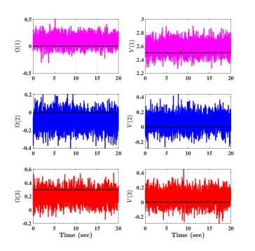
Figure 2: Angular and translational velocities: measured plotted in colored solid-line vs true plotted in black center-line.

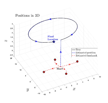
Figure 3: Output performance of the proposed nonlinear stochastic filter for SLAM described in Subsection IV-B and detailed in Algorithm 1 plotted against the true robot’s position and landmark locations in 3D space. The true robot trajectory is plotted in black solid-line with the black circle marking its terminal point. The black circles also mark the true fixed landmarks. Estimation of the robot’s position is plotted as a blue center-line initiating at the origin and converging to its final location marked with a blue star $\star$. Landmark estimation trajectories depicted as red dashed-lines initiate at $(0,0,0)$ and diverge to their final positions marked with red stars $\star$.

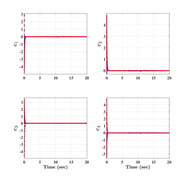
Figure 4: Error trajectories utilized in the Lyapunov function candidate. The proposed nonlinear stochastic estimator for SLAM with IMU outlined in Subsection IV-B is depicted in blue against the deterministic nonlinear estimator for SLAM presented in Subsection IV-A depicted in red.

The asymptotic convergence of the error trajectories of $e_{i}$ achieved by the nonlinear filter for SLAM with IMU (stochastic) and without IMU (deterministic) is demonstrated in Figure 4 for all $i=1,2,3,4$. Consider the error defined as $||\tilde{R}||_{{\rm I}}=\frac{1}{4}{\rm Tr}\{\mathbf{I}_{3}-\tilde{R}\}$ where $\tilde{R}=\hat{R}R^{\top}$, $\tilde{P}=\hat{P}-\tilde{R}P$, and $\tilde{{\rm p}}_{i}=\hat{{\rm p}}_{i}-\tilde{R}{\rm p}_{i}$. It is apparent that $e_{i}=\tilde{{\rm p}}_{i}-\tilde{P}$ does not necessarily result in $||\tilde{R}||_{{\rm I}}\rightarrow 0$, $\tilde{P}\rightarrow 0$, and $\tilde{{\rm p}}_{i}\rightarrow 0$. When designing a SLAM filter, convergence of $\tilde{R}$,$\tilde{P}$, and $\tilde{{\rm p}}_{i}$ to a constant does not constitute the ultimate goal. The true objective is to drive $||\tilde{R}||_{{\rm I}}\rightarrow 0$, $||P-\hat{P}||\rightarrow 0$, and $||{\rm p}_{i}-{\rm\hat{p}}_{i}||\rightarrow 0$. As such, Figure 5 benchmarks the output performance of the proposed stochastic estimator for SLAM with IMU highlighting its superiority over the deterministic solution without IMU. Actually, IMU facilitates achieving $\tilde{R}\rightarrow\mathbf{I}_{3}$ which in turn leads to $||\tilde{R}||_{{\rm I}}\rightarrow 0$ as $t\rightarrow\infty$ significantly reducing error values of $||P-\hat{P}||$ and $||{\rm p}_{i}-{\rm\hat{p}}_{i}||$. This indeed is true as $\tilde{P}=\hat{P}-\tilde{R}P$, and $\tilde{{\rm p}}_{i}=\hat{{\rm p}}_{i}-\tilde{R}{\rm p}_{i}$ causing $\tilde{R}$ to strongly influence the values of $\tilde{P}$ and $\tilde{{\rm p}}_{i}$. Figure 5 reveals the robustness of the proposed stochastic estimator for SLAM using IMU. Figure 5 illustrating its strong convergence as well as tracking capabilities. In contrast, as can be clearly seen in Figure 5, the deterministic nonlinear estimator without IMU shows unreasonable performance in agreement with [7, 8]. It should be noted that presence of the residual error is unavoidable for $||P-\hat{P}||$ and $||{\rm p}_{i}-{\rm\hat{p}}_{i}||$ for the proposed stochastic filter illustrated by Figure 6. Nonetheless, the nonlinear stochastic filter proposed in Subsection IV-B outperforms the nonlinear deterministic filter presented in Subsection IV-A in terms of the convergence rate of $||\tilde{R}||_{{\rm I}}$ and $||P-\hat{P}||$ by a wide margin.

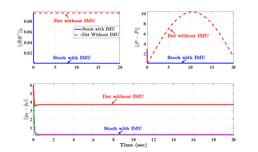
Figure 5: Output performance of $||\hat{R}R^{\top}||_{{\rm I}}$, $||P-\hat{P}||$ and $||{\rm p}_{i}-{\rm\hat{p}}_{i}||$ for all $i=1,2,3,4$. All colors other than red represent the proposed nonlinear stochastic filter based on velocity, landmark, and IMU measurements, while red represents the nonlinear filter based only on velocity and landmark measurements. Det and Stoch abbreviate deterministic and stochastic filters, respectively.

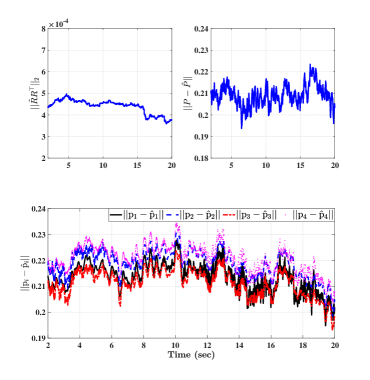
Figure 6: Steady-state values of $||\hat{R}R^{\top}||_{{\rm I}}$, $||P-\hat{P}||$ and $||{\rm p}_{i}-{\rm\hat{p}}_{i}||$ for all $i=1,2,3,4$ of the proposed nonlinear stochastic filter for SLAM.

V-B Experimental Validation

To further validate the proposed nonlinear stochastic estimator for SLAM, the algorithm has been tested on a real-world EuRoc dataset [37]. The data set includes 1) the true orientation and position trajectory of the unmanned aerial vehicle, 2) IMU data, and 3) stereo images. Due to the fact that the dataset does not include landmark information, four landmarks fixed with respect to $\left\{\mathcal{I}\right\}$ have been positioned at ${\rm p}_{1}=[3,0,0]^{\top}$, ${\rm p}_{2}=[-3,0,0]^{\top}$, ${\rm p}_{3}=[0,3,0]^{\top}$, and ${\rm p}_{4}=[0,-3,0]^{\top}$. The four landmark estimates are initiated at the following positions: $\hat{{\rm p}}_{1}\left(0\right)=\hat{{\rm p}}_{2}\left(0\right)=\hat{{\rm p}}_{3}\left(0\right)=\hat{{\rm p}}_{4}\left(0\right)=[0,0,0]^{\top}$. In spite of the large initialization error, Figure 7 demonstrates smooth and continuous convergence of the robot’s position from the origin to the true trajectory successfully arriving to the desired destination. Likewise, Figure 7 shows the convergence of the estimated landmarks from the origin to true locations.

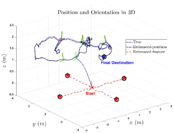
Figure 7: Experimental results using dataset Vicon Room 2 01.

VI Conclusion

To truly capture the nonlinear structure of the motion dynamics of Simultaneous Localization and Mapping (SLAM), a nonlinear stochastic filter for SLAM on the Lie group of $\mathbb{SLAM}_{n}\left(3\right)$ is proposed. The proposed stochastic filter takes into account the unknown constant bias and random noise corrupting the velocity measurements. The proposed filter directly incorporates angular and translational velocity, landmark, and IMU measurements. The closed loop error signals have been shown to be semi-globally uniformly ultimately bounded (SGUUB) in mean square. Numerical results conclusively prove filter’s ability to localize the unknown robot’s pose and simultaneously map the unknown environment.

AUTHOR INFORMATION

Hashim A. Hashim (Member, IEEE) is an Assistant Professor with the Department of Engineering and Applied Science, Thompson Rivers University, Kamloops, British Columbia, Canada. He received the B.Sc. degree in Mechatronics, Department of Mechanical Engineering from Helwan University, Cairo, Egypt, the M.Sc. in Systems and Control Engineering, Department of Systems Engineering from King Fahd University of Petroleum & Minerals, Dhahran, Saudi Arabia, and the Ph.D. in Robotics and Control, Department of Electrical and Computer Engineering at Western University, Ontario, Canada.
His current research interests include stochastic and deterministic attitude and pose filters, Guidance, navigation and control, simultaneous localization and mapping, control of multi-agent systems, and optimization techniques.

References

• [1] S. Thrun et al., “Robotic mapping: A survey,” Exploring artificial intelligence in the new millennium, vol. 1, no. 1-35, p. 1, 2002.
• [2] H. A. Hashim, L. J. Brown, and K. McIsaac, “Nonlinear pose filters on the special euclidean group SE(3) with guaranteed transient and steady-state performance,” IEEE Transactions on Systems, Man, and Cybernetics: Systems, vol. PP, no. PP, pp. 1–14, 2019.
• [3] D. E. Zlotnik and J. R. Forbes, “Higher order nonlinear complementary filtering on lie groups,” IEEE Transactions on Automatic Control, vol. 64, no. 5, pp. 1772–1783, 2018.
• [4] J. Guo, Y. He, X. Qi, G. Wu, Y. Hu, B. Li, and J. Zhang, “Real-time measurement and estimation of the 3d geometry and motion parameters for spatially unknown moving targets,” Aerospace Science and Technology, vol. 97, p. 105619, 2020.
• [5] H. Durrant-Whyte and T. Bailey, “Simultaneous localization and mapping: part i,” IEEE robotics & automation magazine, vol. 13, no. 2, pp. 99–110, 2006.
• [6] V. Sazdovski, A. Kitanov, and I. Petrovic, “Implicit observation model for vision aided inertial navigation of aerial vehicles using single camera vector observations,” Aerospace science and technology, vol. 40, pp. 33–46, 2015.
• [7] H. A. Hashim, “Guaranteed performance nonlinear observer for simultaneous localization and mapping,” IEEE Control Systems Letters, vol. 5, no. 1, pp. 91–96, 2021.
• [8] D. E. Zlotnik and J. R. Forbes, “Gradient-based observer for simultaneous localization and mapping,” IEEE Transactions on Automatic Control, vol. 63, no. 12, pp. 4338–4344, 2018.
• [9] M. Li and B. Xu, “Autonomous orbit and attitude determination for earth satellites using images of regular-shaped ground objects,” Aerospace Science and Technology, vol. 80, pp. 192–202, 2018.
• [10] M. J. Milford and G. F. Wyeth, “Mapping a suburb with a single camera using a biologically inspired slam system,” IEEE Transactions on Robotics, vol. 24, no. 5, pp. 1038–1053, 2008.
• [11] R. Sim, P. Elinas, and J. J. Little, “A study of the rao-blackwellised particle filter for efficient and accurate vision-based slam,” International Journal of Computer Vision, vol. 74, no. 3, pp. 303–318, 2007.
• [12] E. Eade and T. Drummond, “Scalable monocular slam,” in 2006 IEEE Computer Society Conference on Computer Vision and Pattern Recognition (CVPR’06), vol. 1.   IEEE, 2006, pp. 469–476.
• [13] M. Kaess, H. Johannsson, R. Roberts, V. Ila, J. Leonard, and F. Dellaert, “isam2: Incremental smoothing and mapping with fluid relinearization and incremental variable reordering,” in 2011 IEEE International Conference on Robotics and Automation.   IEEE, 2011, pp. 3281–3288.
• [14] G. P. Huang, A. I. Mourikis, and S. I. Roumeliotis, “A quadratic-complexity observability-constrained unscented kalman filter for slam,” IEEE Transactions on Robotics, vol. 29, no. 5, pp. 1226–1243, 2013.
• [15] M. Barczyk, S. Bonnabel, J.-E. Deschaud, and F. Goulette, “Experimental implementation of an invariant extended kalman filter-based scan matching slam,” in 2014 American Control Conference.   IEEE, 2014, pp. 4121–4126.
• [16] G. Dissanayake, S. Huang, Z. Wang, and R. Ranasinghe, “A review of recent developments in simultaneous localization and mapping,” in 2011 6th International Conference on Industrial and Information Systems.   IEEE, 2011, pp. 477–482.
• [17] C. Cadena, L. Carlone, H. Carrillo, Y. Latif, D. Scaramuzza, J. Neira, I. Reid, and J. J. Leonard, “Past, present, and future of simultaneous localization and mapping: Toward the robust-perception age,” IEEE Transactions on robotics, vol. 32, no. 6, pp. 1309–1332, 2016.
• [18] H. A. Hashim, L. J. Brown, and K. McIsaac, “Nonlinear stochastic attitude filters on the special orthogonal group 3: Ito and stratonovich,” IEEE Transactions on Systems, Man, and Cybernetics: Systems, vol. 49, no. 9, pp. 1853–1865, 2019.
• [19] H. A. Hashim, “Systematic convergence of nonlinear stochastic estimators on the special orthogonal group SO(3),” International Journal of Robust and Nonlinear Control, vol. 30, no. 10, pp. 3848–3870, 2020.
• [20] K. J. Jensen, “Generalized nonlinear complementary attitude filter,” Journal of Guidance, Control, and Dynamics, vol. 34, no. 5, pp. 1588–1593, 2011.
• [21] M. Zamani, J. Trumpf, and R. Mahony, “Minimum-energy filtering for attitude estimation,” IEEE Transactions on Automatic Control, vol. 58, no. 11, pp. 2917–2921, 2013.
• [22] H. A. Hashim and F. L. Lewis, “Nonlinear stochastic estimators on the special euclidean group SE(3) using uncertain imu and vision measurements,” IEEE Transactions on Systems, Man, and Cybernetics: Systems, vol. PP, no. PP, pp. 1–14, 2020.
• [23] H. Strasdat, “Local accuracy and global consistency for efficient visual slam,” Ph.D. dissertation, Department of Computing, Imperial College London, 2012.
• [24] T. A. Johansen and E. Brekke, “Globally exponentially stable kalman filtering for slam with ahrs,” in 2016 19th International Conference on Information Fusion (FUSION).   IEEE, 2016, pp. 909–916.
• [25] H. A. Hashim and A. E. E. Eltoukhy, “Landmark and imu data fusion: Systematic convergence geometric nonlinear observer for slam and velocity bias,” IEEE Transactions on Intelligent Transportation Systems, vol. PP, no. PP, pp. 1–10, 2020.
• [26] ——, “Nonlinear filter for simultaneous localization and mapping on a matrix lie group using imu and feature measurements,” IEEE Transactions on Systems, Man, and Cybernetics: Systems, vol. PP, no. PP, pp. 1–12, 2021.
• [27] V. Stojanovic, S. He, and B. Zhang, “State and parameter joint estimation of linear stochastic systems in presence of faults and non-gaussian noises,” International Journal of Robust and Nonlinear Control, vol. 30, no. 16, pp. 6683–6700, 2020.
• [28] R. Khasminskii, Stochastic stability of differential equations.   Rockville, MD: S & N International, 1980.
• [29] A. H. Jazwinski, Stochastic processes and filtering theory.   Courier Corporation, 2007.
• [30] K. Ito and K. M. Rao, Lectures on stochastic processes.   Tata institute of fundamental research, 1984, vol. 24.
• [31] H. Deng, M. Krstic, and R. J. Williams, “Stabilization of stochastic nonlinear systems driven by noise of unknown covariance,” IEEE Transactions on Automatic Control, vol. 46, no. 8, pp. 1237–1253, 2001.
• [32] S. Tong, Y. Li, Y. Li, and Y. Liu, “Observer-based adaptive fuzzy backstepping control for a class of stochastic nonlinear strict-feedback systems,” IEEE Transactions on Systems, Man, and Cybernetics, Part B (Cybernetics), vol. 41, no. 6, pp. 1693–1704, 2011.
• [33] H.-B. Ji and H.-S. Xi, “Adaptive output-feedback tracking of stochastic nonlinear systems,” IEEE Transactions on Automatic Control, vol. 51, no. 2, pp. 355–360, 2006.
• [34] K. W. Lee, W. S. Wijesoma, and J. I. Guzman, “On the observability and observability analysis of slam,” in 2006 IEEE/RSJ International Conference on Intelligent Robots and Systems.   IEEE, 2006, pp. 3569–3574.
• [35] F. Bullo and A. D. Lewis, Geometric control of mechanical systems: modeling, analysis, and design for simple mechanical control systems.   Springer Science & Business Media, 2004, vol. 49.
• [36] H. A. Hashim, “Attitude determination and estimation using vector observations: Review, challenges and comparative results,” arXiv preprint arXiv:2001.03787, 2020.
• [37] M. Burri, J. Nikolic, P. Gohl, T. Schneider, J. Rehder, S. Omari, M. W. Achtelik, and R. Siegwart, “The euroc micro aerial vehicle datasets,” The International Journal of Robotics Research, vol. 35, no. 10, pp. 1157–1163, 2016.