Role of $B_{c}^{+}\to B_{s,d}^{(*)}\,\bar{\ell}\,\nu_{\ell}$ in the Standard Model and in the search for BSM signals

Abstract

The decays $B_{c}^{+}\to B_{a}\bar{\ell}\nu_{\ell}$ and $B_{c}^{+}\to B_{a}^{*}(\to B_{a}\gamma)\bar{\ell}\nu_{\ell}$, with $a=s,d$ and $\ell=e,\mu$, are studied in the Standard Model (SM) and in the extension based on the low-energy Hamiltonian comprising the full set of dimension-$6$ semileptonic $c\to s,d$ operators with left-handed neutrinos. Tests of $\mu/e$ universality are investigated using such modes. The heavy quark spin symmetry is applied to relate the relevant hadronic matrix elements and to exploit lattice QCD results on $B_{c}$ form factors. Optimized observables are selected, and the pattern of their correlations is studied to identify the effects of the various operators in the extended low-energy Hamiltonian.

I Introduction

The $B_{c}$ meson, first observed by the CDF Collaboration [1], is interesting since it has the structure of the heavy quarkonium but it decays weakly. Therefore, this meson is well suited to study both quarkonium and weak interaction features within the same hadronic system. As for weak interactions, in addition to the purely leptonic mode which proceeds through the weak annihilation of the constituent quarks, the $B_{c}$ decays occur through the transitions of both the charm and beauty quark. The decays induced by the charm transition represent the dominant contribution to the full width despite the smaller available phase-space [2, 3, 4, 5]. In our study we focus on the exclusive semileptonic modes $B^{+}_{c}\to B_{s,d}\bar{\ell}\nu_{\ell}$ and $B^{+}_{c}\to B^{*}_{s,d}\bar{\ell}\nu_{\ell}$ induced at the quark level by $c\to(s,d)\bar{\ell}\nu_{\ell}$, with $\ell=e,\mu$ (the tauonic mode is phase-space forbidden). There are various reasons for such a choice.

The first one is the possibility of exploiting the heavy quark spin symmetry [6], which allows us to relate the observables in the modes with final pseudoscalar and vector meson, as well as the different observables in the vector channel. The relatively small phase-space justifies the extrapolation to the full kinematical range of the spin symmetry relations, that strictly hold close to the zero-recoil point where the produced meson is at rest in the $B_{c}$ rest frame [7]. Invoking the heavy quark spin symmetry the relevant hadronic matrix elements can be expressed in terms of two independent functions, that can be derived from the $B_{c}\to B_{s}$ and $B_{c}\to B_{d}$ form factors (FF) precisely determined by lattice QCD [8].

The second reason is the possibility to scrutinize the sensitivity of such processes to beyond the Standard Model (BSM) effects of the kind emerging in $B$ decays, where hints of violation of lepton flavour universality (LFU) are found . The measurement of ${\cal B}(B_{c}\to J/\psi\bar{\tau}\nu_{\tau})$ is also important in this regard [11]. Such effects can be analyzed in an effective theory framework extending the low-energy SM Hamiltonian that governs the $c\to(s,d)\bar{\ell}\nu_{\ell}$ transitions with the inclusion of the full set of semileptonic dimension-$6$ operators with lepton flavour dependent Wilson coefficients. The impact of the new operators on the experimental $B_{c}$ observables can be assessed. The $D$ and $D_{s}$ semileptonic decay modes have been recently studied in this context, and the Wilson coefficients of the new operators in the extended Hamiltonian have been constrained using the available experimental data [12, 13, 14, 15, 16]. The study of the sensitivity of this class of $B_{c}$ decays to extensions of the Standard Model (the New Physics - NP) is timely, as these channels are accessible at the present facilities. The hadronic matrix elements of the new operators can also be given in terms of the same independent functions entering in the SM ones, invoking the heavy quark spin symmetry. Since the produced $B_{s}^{*}$ and $B_{d}^{*}$ mesons decay radiatively, we shall provide the expressions of the fully differential $B_{c}^{+}\to B_{s,d}^{*}(\to B_{s,d}\,\gamma)\bar{\ell}\nu_{\ell}$ decay distribution for the extended low-energy Hamiltonian: such general expressions can also be used for different processes.

In Sec. II we introduce the effective semileptonic Hamiltonian comprising the full set of dimension-6 operators with left-handed neutrinos, that generalizes the SM low-energy Hamiltonian. In Sec. III we provide the decay distributions of $B_{c}\to B_{s,d}\bar{\ell}\nu_{\ell}$ and $B_{c}\to B^{*}_{s,d}(\to B_{s,d}\gamma)\bar{\ell}\nu_{\ell}$ obtained from the extended Hamiltonian. In Sec. IV we discuss the heavy quark spin symmetry relations connecting the SM and NP operator matrix elements. Sec. V contains the numerical analysis in SM and a discussion of the effects of the new operators on the $B_{c}$ decay observables. The summary and the outlook are presented in the last section. The appendices contain the relations among the hadronic form factors obtained by the heavy quark spin symmetry (Appendix A), and the coefficient functions of the full angular distribution of the four-body radiative modes $B_{c}\to B^{*}_{s,d}(\to B_{s,d}\,\gamma)\bar{\ell}\nu_{\ell}$ (Appendix B).

II Effective $c\to s,d$ semileptonic Hamiltonian

We consider the low-energy Hamiltonian comprising the full set of dimension-$6$ semileptonic $Q\to q$ operators with left-handed neutrinos:

$$H_{\rm eff}^{Q\to q\bar{\ell}\nu}=\frac{G_{F}}{\sqrt{2}}V_{CKM}$$

$$\quad\quad\Big{[}(1+\epsilon_{V}^{\ell})\left({\bar{q}}\gamma_{\mu}(1-\gamma_{5})Q\right)\left(\bar{\nu}_{\ell}(1+\gamma_{5})\gamma^{\mu}\ell\right)$$

$$\quad\quad+\epsilon_{R}^{\ell}\left({\bar{q}}\gamma_{\mu}(1+\gamma_{5})Q\right)\left(\bar{\nu}_{\ell}(1+\gamma_{5})\gamma^{\mu}\ell\right)$$

$$\quad\quad+\epsilon_{S}^{\ell}\,({\bar{q}}Q)\left({\bar{\nu}_{\ell}}(1+\gamma_{5})\ell\right)$$ (1)

$$\quad\quad+\epsilon_{P}^{\ell}\,\left({\bar{q}}\gamma_{5}Q\right)\left({\bar{\nu}_{\ell}}(1+\gamma_{5})\ell\right)$$

$$\quad\quad+\epsilon_{T}^{\ell}\,\left({\bar{q}}(1+\gamma_{5})\sigma_{\mu\nu}Q\right)\,\left({\bar{\nu}_{\ell}}(1+\gamma_{5})\sigma^{\mu\nu}\ell\right)\Big{]},$$

with $Q=c$, and $q$ either the $s$ or the $d$ quark. $V_{CKM}$ is the Cabibbo-Kobayashi-Maskawa (CKM) matrix element $V_{cs}$ or $V_{cd}$. In addition to the SM operator ${\cal O}_{SM}=4(\bar{q}_{L}\gamma^{\mu}Q_{L})\left({\bar{\nu}_{\ell L}}\gamma_{\mu}\ell_{L}\right)$ and to the operators ${\cal O}_{S}=\left({\bar{q}}Q\right)\left({\bar{\nu}_{\ell}}(1+\gamma_{5})\ell\right)$, ${\cal O}_{P}=\left({\bar{q}}\gamma_{5}Q\right)\left({\bar{\nu}_{\ell}}(1+\gamma_{5})\ell\right)$ and ${\cal O}_{T}=\left({\bar{q}}(1+\gamma_{5})\sigma_{\mu\nu}Q\right)\left({\bar{\nu}_{\ell}}(1+\gamma_{5})\sigma^{\mu\nu}\ell\right)$, the operator ${\cal O}_{R}=4(\bar{q}_{R}\gamma^{\mu}Q_{R})\left({\bar{\nu}_{\ell L}}\gamma_{\mu}\ell_{L}\right)$ is included in Eq. (1). It is worth remarking that in the Standard Model Effective Field Theory the only dimension-$6$ operator with the right-handed quark current is nonlinear in the Higgs field [17, 18, 19], and its role has been the subject of several discussions [20, 21, 22, 23, 24, 19]. The complex coefficients $\epsilon^{\ell}_{V,R,S,P,T}$ in the low-energy Hamiltonian (1) are lepton-flavour dependent.

Generalized Hamiltonians as in Eq. (1) have been studied for $b\to c$ transitions in connection with the anomalies in semileptonic $B\to D^{(*)}\tau\nu_{\tau}$ decays, obtaining information on the various operators [25, 26, 27, 28, 29, 30, 31, 32]. Modes induced by the $b\to u$ induced transition have also been analyzed in such an effective theory approach [33]. For both classes of $b$-quark transitions, suitable observables testing the Standard Model and challenging LFU have been identified. Observables in baryon decays, in particular in inclusive modes, have also been studied [34]. Here we focus on the $B_{c}$ decays governed by the Hamiltonian (1), to study the SM phenomenology and to assess the sensitivity of such channels to deviations from the SM.

III Modes $B_{c}\to P\,\bar{\ell}\nu_{\ell}$ and $B_{c}\to V(\to P\gamma)\,\bar{\ell}\nu_{\ell}$

The $q^{2}$ distribution of the $B_{c}\to P\bar{\ell}\nu_{\ell}$ decay, with $P$ a pseudoscalar meson, governed by the low-energy Hamiltonian (1) reads:

$$\frac{d\Gamma(B_{c}\to P\bar{\ell}{\nu}_{\ell})}{dq^{2}}=$$

$$\frac{G_{F}^{2}|V_{CKM}|^{2}\lambda^{1/2}}{128\,m_{B_{c}}^{3}\pi^{3}q^{2}}\left(1-\frac{m_{\ell}^{2}}{q^{2}}\right)^{2}$$

$$\Bigg{\{}\left|m_{\ell}(1+\epsilon_{V}^{\ell}+\epsilon_{R}^{\ell})+\frac{q^{2}\epsilon_{S}^{\ell}}{m_{Q}-m_{q}}\right|^{2}(m_{B_{c}}^{2}-m_{P}^{2})^{2}f_{0}^{2}(q^{2})$$

$$+\lambda\Bigg{[}\frac{1}{3}\left|m_{\ell}(1+\epsilon_{V}^{\ell}+\epsilon_{R}^{\ell})f_{+}(q^{2})+\frac{4q^{2}}{m_{B_{c}}+m_{P}}\epsilon_{T}^{\ell}f_{T}(q^{2})\right|^{2}$$

$$+\frac{2q^{2}}{3}\left|(1+\epsilon_{V}^{\ell}+\epsilon_{R}^{\ell})f_{+}(q^{2})+4\frac{m_{\ell}}{m_{B_{c}}+m_{P}}\epsilon_{T}^{\ell}f_{T}(q^{2})\right|^{2}\Bigg{]}\Bigg{\}}.$$

(2)

$G_{F}$ is the Fermi constant, $q^{2}$ the squared momentum transferred to the lepton pair and $\lambda=\lambda(m_{B_{c}}^{2},m_{P}^{2},q^{2})$ is the triangular function. The form factors $f_{+}$, $f_{0}$ and $f_{T}$ are defined in Appendix A. The SM expression is recovered setting to zero all couplings $\epsilon_{i}^{\ell}$.

In the case of a final vector meson $V$ decaying to $P\gamma$, namely $B^{*}_{s,d}$, the four-body kinematics of $B_{c}\to V(\to P\gamma)\,\bar{\ell}\nu_{\ell}$ is shown in Fig. 1.

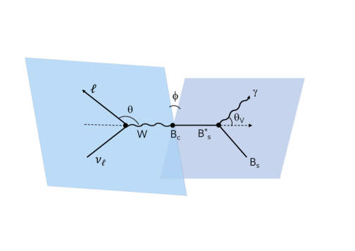
Figure 1: Kinematics of the $B_{c}\to B_{s}^{*}(B_{s}\gamma)\bar{\ell}\nu_{\ell}$ decay.

The fully differential decay width is expressed in terms of $q^{2}$ and of the angles $\theta_{V}$, $\theta$ and $\phi$ defined in the figure:

$$\frac{d^{4}\Gamma(B_{c}\to V(\to P\gamma)\bar{\ell}\nu_{\ell})}{dq^{2}\,d\cos\theta_{V}\,d\cos\theta\,d\phi}={\cal N_{\gamma}}|{\vec{p}}_{V}|\left(1-\frac{m_{\ell}^{2}}{q^{2}}\right)^{2}$$

$$\quad\quad\Big{\{}I_{1s}\,\sin^{2}\theta_{V}+I_{1c}\,(3+\cos 2\theta_{V})$$

$$\quad\quad+(I_{2s}\,\sin^{2}\theta_{V}+I_{2c}\,(3+\cos 2\theta_{V}))\cos 2\theta$$

$$\quad\quad+I_{3}\,\sin^{2}\theta_{V}\sin^{2}\theta\cos 2\phi+I_{4}\sin 2\theta_{V}\sin 2\theta\cos\phi$$

$$\quad\quad+I_{5}\,\sin 2\theta_{V}\sin\theta\cos\phi$$ (3)

$$\quad\quad+(I_{6s}\,\sin^{2}\theta_{V}+I_{6c}\,(3+\cos 2\theta_{V}))\cos\theta$$

$$\quad\quad+I_{7}\sin 2\theta_{V}\sin\theta\sin\phi+I_{8}\sin 2\theta_{V}\sin 2\theta\sin\phi$$

$$\quad\quad+I_{9}\,\sin^{2}\theta_{V}\sin^{2}\theta\sin 2\phi\Big{\}},$$

with $|{\vec{p}}_{V}|=\sqrt{\lambda(m_{B_{c}}^{2},m_{V}^{2},q^{2})}/2m_{B_{c}}$. The distribution (3) is obtained in the narrow width approximation for the meson $V$, and the factor ${\cal N}_{\gamma}=\displaystyle{\frac{3G_{F}^{2}|V_{CKM}|^{2}{\cal B}(V\to P\gamma)}{128(2\pi)^{4}m_{B_{c}}^{2}}}$ comprises the $V\to P\gamma$ branching fraction. The angular coefficient functions $I_{i}(q^{2})$ encode the dynamics and the SM and of NP described by the Hamiltonian (1). We provide them for the full set of operators, generalizing the results obtained in [30] for the tensor operator:

$$I_{i} = |1+\epsilon_{V}|^{2}\,I_{i}^{SM}+|\epsilon_{R}|^{2}I_{i}^{NP,R}+|\epsilon_{P}|^{2}I_{i}^{NP,P}\hskip 28.45274pt$$

$$+ |\epsilon_{T}|^{2}I_{i}^{NP,T}+2\,{\rm Re}\left[\epsilon_{R}(1+\epsilon_{V}^{*})\right]I_{i}^{INT,R}$$

$$+ 2\,{\rm Re}\left[\epsilon_{P}(1+\epsilon_{V}^{*})\right]I_{i}^{INT,P}$$

$$+ 2\,{\rm Re}\left[\epsilon_{T}(1+\epsilon_{V}^{*})\right]I_{i}^{INT,T}$$

$$+ 2\,{\rm Re}\left[\epsilon_{R}\epsilon_{T}^{*}\right]I_{i}^{INT,RT}+2\,{\rm Re}\left[\epsilon_{P}\epsilon_{T}^{*}\right]I_{i}^{INT,PT}$$

$$+ 2\,{\rm Re}\left[\epsilon_{P}\epsilon_{R}^{*}\right]I_{i}^{INT,PR}$$

for $i=1,\dots 6$,

$$I_{7} = 2\,{\rm Im}\left[\epsilon_{R}(1+\epsilon_{V}^{*})\right]I_{7}^{INT,R}$$

$$+ 2\,{\rm Im}\left[\epsilon_{P}(1+\epsilon_{V}^{*})\right]I_{7}^{INT,P}$$

$$+ 2\,{\rm Im}\left[\epsilon_{T}(1+\epsilon_{V}^{*})\right]I_{7}^{INT,T}$$

$$+ 2\,{\rm Im}\left[\epsilon_{R}\epsilon_{T}^{*}\right]I_{7}^{INT,RT}+2\,{\rm Im}\left[\epsilon_{P}\epsilon_{T}^{*}\right]I_{7}^{INT,PT}\quad\quad$$

$$+ 2\,{\rm Im}\left[\epsilon_{P}\epsilon_{R}^{*}\right]I_{7}^{INT,PR},$$

and

$$I_{i}=2\,{\rm Im}\left[\epsilon_{R}(1+\epsilon_{V}^{*})\right]I_{i}^{INT,R}$$ (6)

for $i=8,\,9$. In SM the angular coefficient functions are given in terms of the helicity amplitudes

$$H_{0} = \frac{1}{{2m_{V}(m_{B_{c}}+m_{V})\sqrt{q^{2}}}}$$ (7)

$$\Big{(}(m_{B_{c}}+m_{V})^{2}(m_{B_{c}}^{2}-m_{V}^{2}-q^{2})A_{1}(q^{2})$$

$$- \lambda(m_{B_{c}}^{2},\,m_{V}^{2},\,q^{2})A_{2}(q^{2})\Big{)}$$

$$H_{\pm} = \frac{(m_{B_{c}}+m_{V})^{2}A_{1}(q^{2})\mp\sqrt{\lambda(m_{B_{c}}^{2},\,m_{V}^{2},\,q^{2})}V(q^{2})}{m_{B_{c}}+m_{V}}$$

$$H_{t} = -\frac{\sqrt{\lambda(m_{B_{c}}^{2},\,m_{V}^{2},\,q^{2})}}{\sqrt{q^{2}}}\,A_{0}(q^{2}).\,\,\,$$

For the NP operators the following amplitudes are also introduced:

$$H_{\pm}^{NP} = \frac{1}{\sqrt{q^{2}}}\Big{\{}\Big{(}m_{B_{c}}^{2}-m_{V}^{2}\pm\sqrt{\lambda(m_{B_{c}}^{2},m_{V}^{2},q^{2})}\Big{)}(T_{1}+T_{2})$$

$$+ q^{2}(T_{1}-T_{2})\Big{\}}$$

$$H_{L}^{NP} = 4\Big{\{}\frac{\lambda(m_{B_{c}}^{2},m_{V}^{2},q^{2})}{m_{V}(m_{B_{c}}+m_{V})^{2}}\,T_{0}+2\frac{m_{B_{c}}^{2}+m_{V}^{2}-q^{2}}{m_{V}}T_{1}$$ (8)

$$+ 4m_{V}T_{2}\Big{\}}.$$

The form factors $V$, $A_{i}$ and $T_{i}$ are defined in Appendix A. The coefficient functions in Eqs. (III), (III) and (6), expressed in terms of the amplitudes (7) and (8), are collected in Appendix B. With such expressions the various observables can be computed by suitable integrations of the distribution in Eq. (3).

IV Heavy quark spin symmetry and relations among form factors

In the infinite heavy quark mass limit $m_{Q}\gg\Lambda_{\rm QCD}$ the QCD Lagrangian exhibits a heavy quark (HQ) spin symmetry, with the decoupling of the heavy quark spin from gluons [35]. This produces the decoupling of the spins of the heavy quarks in $B_{c}$: the spin-spin interaction vanishes in this limit. Important consequences of the HQ spin symmetry are the relations among the form factors parametrizing the weak current matrix elements of $B_{c}$ and mesons comprising a single heavy quark ($B_{s}^{(*)},B_{d}^{(*)},D^{(*)},\dots$) or two heavy quarks ($\eta_{c},J/\psi,\psi(2S),\dots$) [6].

In the semileptonic $B_{c}\to B_{a}^{(*)}$ ($a=s,d$) decays induced by the $c\to s,d$ transition, since $m_{c}\ll m_{b}$ the energy released to the final hadronic system is much smaller than $m_{b}$. The $b$ quark remains almost unaffected, so that the final meson keeps the same $B_{c}$ four-velocity $v$. Denoting the initial and final meson four-momenta as $p=m_{B_{c}}v$ and $p^{\prime}=m_{B_{a}}v^{\prime}=m_{B_{a}}v+k$ , with $k$ a small residual momentum, the four-momentum transferred to the leptons is $q=p-p^{\prime}=(m_{B_{c}}-m_{B_{a}})v-k$, with $v\cdot k={\cal O}(1/m_{b})$.

The relations stemming from the HQ spin symmetry can be worked out using the trace formalism [36]. The heavy pseudoscalar and vector mesons are collected in doublets, the two components of which represent states differing only for the orientation of the heavy quark spins. The $B_{c}^{+}$ and $B_{c}^{*+}$ doublet comprising the heavy $c$ and $\bar{b}$ quarks is described by the effective fields

$$H^{c\bar{b}}=\frac{1+\not\!v\,}{2}\left[B_{c}^{*\mu}\gamma_{\mu}-B_{c}\gamma_{5}\right]\frac{1-\not\!v\,}{2}.$$ (9)

The $B_{a}$ and $B_{a}^{*}$ doublet ($a$ an $SU(3)_{F}$ index) with the single heavy antiquark $\bar{b}$ is described by the effective fields

$$H^{\bar{b}}=\left[B_{a}^{*\mu}\gamma_{\mu}-B_{a}\gamma_{5}\right]\frac{1-\not\!v\,}{2}.$$ (10)

$B$ and $B^{*}$ are operators that include a factor $\sqrt{m_{B}}$ and $\sqrt{m_{B}^{*}}$ and have dimension $3/2$. The equations ${\not\!v\,}H^{c\bar{b}}=H^{c\bar{b}}$, $\ H^{c\bar{b}}{\not\!v\,}=-H^{c\bar{b}}$, ${\not\!v\,}H^{\bar{b}}=H^{\bar{b}}$, $\ H^{\bar{b}}{\not\!v\,}=-H^{\bar{b}}$ are satisfied. Under the heavy quark spin transformations and light quark $SU(3)_{F}$ transformations the doublets transform as

$$H^{c\bar{b}}\to S_{c}H^{c\bar{b}}S^{\dagger}_{b}$$

$$H^{\bar{b}}_{a}\to(UH^{\bar{b}})_{a}S^{\dagger}_{b}.$$ (11)

The matrix elements of the quark current ${\bar{q}}\Gamma Q$ between $B_{c}$ and $B_{a}^{(*)}$, with $\Gamma$ a generic product of Dirac matrices, can be written as

$$\langle B_{a}^{(*)}(v,k)|{\bar{q}}\Gamma Q|{B_{c}}(v)\rangle=$$

$$-\sqrt{m_{B_{c}}m_{B_{a}}}\,{\rm Tr}\left[\overline{H}_{a}^{(\bar{b})}\Omega_{a}(v,a_{0}k)\Gamma H^{(c\bar{b})}\right],$$ (12)

with $\overline{H}_{a}=\gamma^{0}H_{a}^{\dagger}\gamma^{0}$ and are invariant under rotations of the $\bar{b}$ spin. The most general matrix depending on $v$ and $k$ is

$$\Omega_{a}(v,a_{0}k)=\Omega_{1a}+\not\!k\,a_{0}\Omega_{2a}.$$ (13)

It involves two dimensionless nonperturbative functions, the form factors $\Omega_{1a}$ and $\Omega_{2a}$. The dimensionful parameter $a_{0}$ can be identified with the length scale of the process, typically the Bohr radius of the mesons. At odds with the weak matrix elements of mesons comprising a single heavy quark, that are expressed in terms of a single universal function (the Isgur-Wise function [37, 38]) normalized to 1 at the zero-recoil point $v\cdot v^{\prime}=1$ due to the heavy quark flavour symmetry, no normalization is fixed for $\Omega_{1}$ and $\Omega_{2}$. Such form factors encode the QCD dynamics and must be determined by nonperturbative methods.

The SM matrix elements relevant for $B_{c}^{+}\to B_{a}\ell^{+}{\nu}_{\ell}$ involve the form factors $f_{+}^{B_{c}\to P_{a}}$ and $f_{0}^{B_{c}\to P_{a}}$ defined in (A.1). On the other hand, four form factors are needed in SM for each $B_{c}\to B_{a}^{*}\ell{\bar{\nu}}_{\ell}$ mode, $V^{B_{c}\to V_{a}}$ and $A_{1,2,0}^{B_{c}\to V_{a}}$ defined in (A.2). They parametrize the hadronic matrix elements of the SM operator in the low-energy Hamiltonian (1). The matrix elements of the operators with a scalar and pseudoscalar quark current in Eq. (1) do not involve new form factors: the scalar operator contributes only to $B_{c}\to B_{a}\ell{\bar{\nu}}_{\ell}$ and its hadronic matrix element is given in terms of $f_{0}^{B_{c}\to B_{a}}$ and of the masses of the quarks involved in the transitions. The pseudoscalar operator contributes only to $B_{c}\to B_{a}^{*}\ell{\bar{\nu}}_{\ell}$ and its matrix element can be expressed in terms of $A_{0}^{B_{c}\to B_{a}^{*}}$ and the quark masses (Appendix A). The matrix elements of the tensor operator in (1) require the form factors $f_{T}^{B_{c}\to B_{a}}$ for $B_{c}^{+}\to B_{a}\ell^{+}{\nu}_{\ell}$ and $T_{1,2,0}^{B_{c}\to B_{a}^{*}}$ for $B_{c}^{+}\to B_{a}^{*}\ell^{+}{\nu}_{\ell}$ defined in Appendix A.

Exploiting the HQ spin symmetry all the form factors $f_{+},\,f_{0},\,f_{T}$ and $V,A_{i},T_{i}$ can be given in terms of the functions $\Omega_{1,2}$ in (13). Such relations can be inverted to express $\Omega_{1}$ and $\Omega_{2}$ in terms of $f_{+}$ and $f_{0}$, Eq. (LABEL:eq:om12), and can be used once such functions are determined in a nonperturbative way. All relations are in Appendix A. The result is that $f_{+}$ and $f_{0}$, accompanied with the relations from the HQ spin symmetry, provide enough information to study the full phenomenology of the $B_{c}\to B^{(*)}_{a}$ semileptonic modes in SM and beyond.

The relations among the form factors are valid close to the zero-recoil point, at maximum momentum squared transferred to the lepton pair $q^{2}_{max}=(m_{B_{c}}-m_{B_{a}^{(*)}})^{2}$. However, since the phase space for $B_{c}\to B_{a}^{(*)}$ is small, such relations can be extrapolated to the full kinematical $q^{2}$ range. The assumption can be checked once other form factors are available, by a comparison with the expressions in the heavy quark limit.

V Numerical analysis

We describe several observables in $B_{c}^{+}\to B_{s,d}\ell^{+}\nu_{\ell}$ and $B_{c}^{+}\to B_{s,d}^{*}(\to B_{s,d}\gamma)\ell^{+}\nu_{\ell}$ in the Standard Model. We also study their sensitivity to the BSM operators in the low-energy Hamiltonian.

For the hadronic matrix elements of the various operators in Eq. (1) we exploit the HQ spin symmetry and express all form factors in terms of the universal functions $\Omega_{1s(d)}$ and $\Omega_{2s(d)}$ using the relations in Appendix A. $\Omega_{1s(d)}$ and $\Omega_{2s(d)}$ are determined from the form factors $f_{+,0}^{B_{c}\to B_{s}}$ and $f_{+,0}^{B_{c}\to B_{d}}$ computed by lattice QCD in Ref. [8]. In such computation the form factors are evaluated in the full $q^{2}$ range, by a chain fit of the results obtained by a non-relativistic QCD treatment of the $b$ quark and by using the highly improved staggered quark method. The variable $t=q^{2}$, with kinematical bound $m_{\ell}^{2}\leq t\leq t_{-}=(m_{B_{c}}-m_{B_{s(d)}})^{2}$, is mapped into the variable $z(t)=\frac{\sqrt{t_{+}-t}-\sqrt{t}_{+}}{\sqrt{t_{+}-t}+\sqrt{t}_{+}}$ with $t_{+}=(m_{B_{c}}+m_{B_{s(d)}})^{2}$ chosen to be larger than the lowest threshold for hadron production in the $t$ channel, the $DK$ and $D\pi$ threshold. To optimize the calculation, a rescaled variable $z_{p}(t)=z(t)/z(M^{2}_{res})$ is defined, with $M_{res}$ a suitably chosen mass parameter. Each form factor $f(t)$ is expressed (in the continuum limit of the lattice discretization) as a truncated power series of $z_{p}$:

$$f(t)=P(t)\sum_{n}^{N}A_{n}z_{p}(t)^{n}\,\,,$$ (14)

with $P(t)$ a function chosen to describe the main computed $t$-dependence. As a result, each form factor is determined by the set of coefficients $A_{n}$ together with their errors and error correlation matrices. The functions $\Omega_{1}(y)$ and $a_{0}\Omega_{2}(y)$ obtained for the $c\to s$ and $c\to d$ transitions are depicted in Fig. 2 together with their uncertainties. They are expressed in terms of the variable $y=\displaystyle\frac{p\cdot p^{\prime}}{m_{B_{c}}m_{B_{a}}}=\frac{m_{B_{c}}^{2}+m_{B_{a}}^{2}-q^{2}}{2m_{B_{c}}m_{B_{a}}}$ in the range $[1,y_{max}]$, with $y_{max}$ corresponding to $q^{2}_{min}=m_{\ell}^{2}$. The numerical values of the other parameters, taken from the Particle Data Group [39], are listed in Table 1.

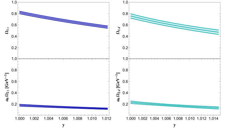
Figure 2: Universal functions $\Omega_{1}(y)$ (top) and $a_{0}\Omega_{2}(y)$ (bottom panels) obtained using Eq. (LABEL:eq:om12) and the form factors $f_{+}$ and $f_{0}$ computed in Ref. [8] for $B_{c}\to B_{s}$ (left) and $B_{c}\to B_{d}$ matrix elements (right panels), with $\displaystyle y=\frac{p\cdot p^{\prime}}{m_{B_{c}}m_{B_{a}}}$.

Table 1: Parameters, from Ref. [39].

$m_{B_{c}}$	$6274.9\pm 0.8$ MeV
$\tau_{B_{c}}$	$(0.510\pm 0.009)\times 10^{-12}$ s
$m_{B_{s}}$	$5366.88\pm 0.14$ MeV
$m_{B_{s}^{*}}$	$5415.8\pm 1.5$ MeV
${\cal B}(B_{s}^{*}\to B_{s}\gamma)$	1
$m_{B_{d}}$	$5279.63\pm 0.20$ MeV
$m_{B_{d}^{*}}$	$5324.7\pm 0.21$ MeV
${\cal B}(B_{d}^{*}\to B_{d}\gamma)$	1
$|V_{cs}|$	$0.987\pm 0.011$
$|V_{cd}|$	$0.221\pm 0.004$
$m_{d}^{\overline{MS}}(2\,GeV)$	$4.67^{+0.48}_{-0.17}$ MeV
$m_{s}^{\overline{MS}}(2\,GeV)$	$93^{+11}_{-5}$ MeV
$m_{c}$	$1.67\pm 0.07$ GeV

The analysis of the sensitivity to the BSM operators in Eq. (1) requires a set of input values for the coefficients $\epsilon_{i}^{\ell}$. There are experimental constraints, in particular from the purely leptonic $D_{s}$ and $D^{+}$ decay widths, from the semileptonic $D^{0(+)}$ decays to $K^{-(0)},K^{*-(0)}$ and $\pi^{-(0)},\rho^{-(0)}$, and from the semileptonic $D_{s}\to\phi$ transitions [12, 13, 15, 16]. Ranges of values have been determined upon the assumption that all $\epsilon_{i}^{\ell}$ are real [16]: $\epsilon_{V}^{\mu}=(1.65\pm 2.02)\times 10^{-2}$, $\epsilon_{R}^{\mu}=(-1.35\pm 2.02)\times 10^{-2}$, $\epsilon_{S}^{\mu}=(-1.0\pm 2.0)\times 10^{-2}$, $\epsilon_{P}^{\mu}=(0.9\pm 1.4)\times 10^{-3}$ and $\epsilon_{T}^{\mu}=(1.2\pm 1.8)\times 10^{-2}$ for the $c\to s$ transition, and $\epsilon_{V}^{\mu}=(5.0\pm 2.1)\times 10^{-2}$, $\epsilon_{R}^{\mu}=(2.0\pm 2.0)\times 10^{-2}$, $\epsilon_{S}^{\mu}=(-9.0\pm 7.0)\times 10^{-2}$, $\epsilon_{P}^{\mu}=(-2.6\pm 1.3)\times 10^{-3}$ and $\epsilon_{T}^{\mu}=(-2.0\pm 1.4)\times 10^{-1}$ for the $c\to d$ transition. Interestingly, the allowed range for $\epsilon_{T}^{\mu}$ in the $c\to d$ transition is wide. We vary the couplings in these intervals with the purpose of describing the effects of the various NP operators. Assuming a hierarchy in LFU violation, all couplings for the electron operators $\epsilon^{e}_{V,R,S,P,T}$ are kept to zero, hence such modes are only described in SM.

V.1 $B_{c}\to B_{s}\ell^{-}\bar{\nu}_{\ell}$ and $B_{c}\to B_{s}^{*}(\to B_{s}\gamma)\ell^{-}\bar{\nu}_{\ell}$

The semileptonic $B_{c}$ decays induced by the $c\to s$ transition are expected to constitute the largest fraction of semileptonic modes [7, 40, 41, 42, 43, 44, 45, 46, 47, 48, 49, 50]. The prediction in SM

$${\cal B}(B_{c}^{+}\to B_{s}\,\mu^{+}\nu_{\mu})=0.0125\,(4)\,\left(\frac{|V_{cs}|}{0.987}\right)^{2}\,\,$$ (15)

follows from the use of form factors in [8]. The quoted error refers only to the form factor uncertainties, the errors from the CKM matrix element and from the $B_{c}$ lifetime in Table 1 can be simply added, the error from the mass parameters is small. For the electron mode the result is:

$${\cal B}(B_{c}^{+}\to B_{s}\,e^{+}\nu_{e})=0.0131\,(4)\,\left(\frac{|V_{cs}|}{0.987}\right)^{2}.$$ (16)

In the case of $\mu$ we describe below how the branching fraction changes due to the NP operators, studying also the correlation with other observables. We notice that the $q^{2}$ spectrum in Fig. 3 is modified with respect to the Standard Model when the additional operators in (1) are considered. The SM prediction including the FF uncertainty is enlarged if the NP operators are considered, varying the couplings $\epsilon_{i}^{\mu}$ in their quoted ranges. However, the shape of the spectrum is unchanged.

For $B_{c}^{+}\to B_{a}^{*}\mu^{+}\nu_{\mu}$ ($a=s,d$), the SM helicity amplitudes (7) can be expressed in terms of $\Omega_{1a}$ and $\Omega_{2a}$:

$$H_{0} = \sqrt{\frac{m_{B_{c}}}{m_{B_{a}^{*}}}}\frac{(m_{B_{c}}^{2}-m_{B_{a}^{*}}^{2}-q^{2})}{\sqrt{q^{2}}}\Omega_{1a}$$

$$+ \frac{\lambda(m_{B_{c}}^{2},m_{B_{a}^{*}}^{2},q^{2})}{2\sqrt{m_{B_{c}}m_{B_{a}^{*}}q^{2}}}\,a_{0}\Omega_{2a}$$

$$H_{\pm} = \sqrt{\frac{m_{B_{a}^{*}}}{m_{B_{c}}}}\bigg{(}2m_{B_{c}}\Omega_{1a}$$ (17)

$$\mp \lambda^{1/2}(m_{B_{c}}^{2},m_{B_{a}^{*}}^{2},q^{2})\,a_{0}\Omega_{2a}\bigg{)}$$

$$H_{t} = -\frac{\lambda^{1/2}(m_{B_{c}}^{2},m_{B_{a}^{*}}^{2},q^{2})}{2\sqrt{m_{B_{c}}m_{B_{a}^{*}}q^{2}}}\bigg{(}2m_{B_{c}}\Omega_{1a}$$

$$+ (m_{B_{c}}^{2}-m_{B_{a}^{*}}^{2}+q^{2})\,a_{0}\Omega_{2a}\bigg{)},$$

while the NP amplitudes (8) read:

$$H_{\pm}^{NP} = 2\,\sqrt{\frac{m_{B^{*}_{a}}}{m_{B_{c}}q^{2}}}$$

$$\bigg{[} \bigg{(}m_{B_{c}}^{2}-m_{B^{*}_{a}}^{2}+q^{2}\pm\sqrt{\lambda(m_{B_{c}}^{2},m_{B^{*}_{a}}^{2},q^{2})}\bigg{)}\,\Omega_{1}$$

$$+ \bigg{(}(m_{B_{c}}+m_{B^{*}_{a}})\,\big{(}(m_{B_{c}}-m_{B^{*}_{a}})^{2}-q^{2}\big{)}$$

$$\pm (m_{B_{c}}-m_{B^{*}_{a}})\,\sqrt{\lambda(m_{B_{c}}^{2},m_{B^{*}_{a}}^{2},q^{2})}\bigg{)}\,a_{0}\,\Omega_{2}\bigg{]}$$

$$H_{L}^{NP} = \frac{16}{\sqrt{m_{B_{c}}m_{B^{*}_{a}}}}\,\bigg{[}(m_{B_{c}}^{2}+m_{B^{*}_{a}}^{2}-q^{2})\,\Omega_{1}$$

$$- m_{B^{*}_{a}}\,\big{(}(m_{B_{c}}-m_{B^{*}_{a}})^{2}-q^{2}\big{)}\,a_{0}\,\Omega_{2}\bigg{]}\;.$$

For $a=s$ the SM predictions

$${\cal B}(B_{c}^{+}\to B_{s}^{*}\,\mu^{+}\nu_{\mu}) = \,0.030\,(1)\,\,\left(\frac{|V_{cs}|}{0.987}\right)^{2}$$

$${\cal B}(B_{c}^{+}\to B_{s}^{*}\,e^{+}\nu_{e}) = \,0.032\,(1)\,\,\left(\frac{|V_{cs}|}{0.987}\right)^{2}$$ (19)

include only the error on the form factors. For $\mu$ channel, the $q^{2}$ distribution in Fig. 3 is affected by a small FF uncertainty. In the NP extension the tensor operator has a visible effect on the spectrum. Moreover, the spectra of longitudinally and transversely polarized $B_{s}^{*}$ in Fig. 4 show that NP mainly affects the longitudinal $B^{*}_{s}$ polarization in the small $q^{2}$ region. The ratio $\displaystyle F_{T}=\frac{\Gamma_{T}}{\Gamma_{L}+\Gamma_{T}}$, with $\Gamma_{T,L}$ the decay widths to transversely and longitudinally polarized $B_{s}^{*}$, is predicted in the SM: $F_{T}=0.413\pm 0.004$, and remains smaller than $1/2$ when the NP operators are included, with the main effect due to the $T$ operator, as shown in Fig. 5.

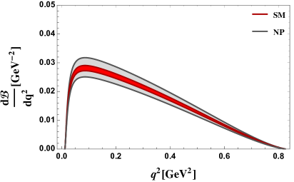
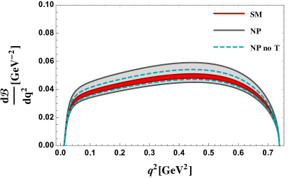
Figure 3: $q^{2}$ spectrum of the modes $B_{c}^{+}\to B_{s}\mu^{+}\nu_{\mu}$ (top) and $B_{c}^{+}\to B_{s}^{*}\mu^{+}\nu_{\mu}$ (bottom). The Standard Model result (red SM band) includes the uncertainty on the form factors. The result for the full Hamiltonian Eq. (1) is obtained varying the effective couplings in the quoted ranges (gray NP band). For $B_{c}^{+}\to B_{s}^{*}\mu^{+}\nu_{\mu}$ the spectrum obtained omitting the tensor operator $T$ is also displayed (dashed cyan lines).

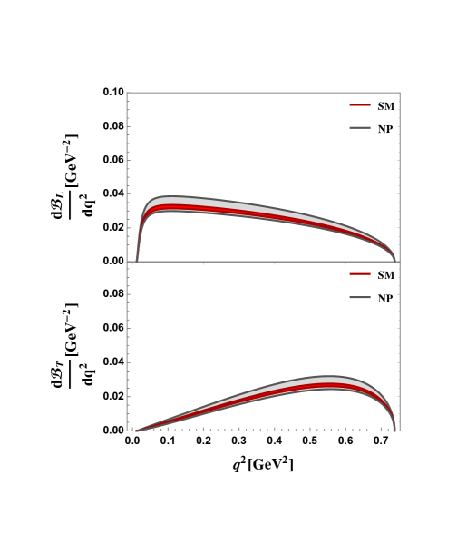
Figure 4: $q^{2}$ distribution for longitudinally (top) and transversely polarized $B_{s}^{*}$ meson (bottom) in $B_{c}^{+}\to B_{s}^{*}\mu^{+}\nu_{\mu}$. The color codes are the same as in Fig. 3.

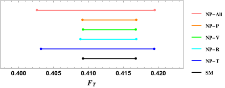
Figure 5: Fraction of transversely polarized $B_{s}^{*}$. The lines correspond to SM, to the NP operators in Eq. (1) separately considered, and to the full set of NP operators.

The $q^{2}$-dependent forward-backward (FB) lepton asymmetry

$${\cal A_{FB}}(q^{2})=\left({\displaystyle{\frac{d\Gamma}{dq^{2}}}}\right)^{-1}\times$$ (20)

$$\left[\int_{0}^{1}\,d\cos\,\theta\,\displaystyle{\frac{d^{2}\Gamma}{dq^{2}d\cos\,\theta}}-\int_{-1}^{0}\,d\cos\,\theta\,\displaystyle{\frac{d^{2}\Gamma}{dq^{2}d\cos\,\theta}}\right]\,\,\,$$

is affected by a small uncertainty in the SM (Fig. 6). The asymmetry has a zero precisely determined at $q_{0}^{2}\simeq 0.1905\,(5)$ GeV². This observable is particular sensitive to the tensor operator: indeed, as shown in Fig. 6, excluding this operator the asymmetry in NP practically coincides with SM. When all the operators in the extended Hamiltonian are considered the position of the zero is in the range $q_{0}^{2}\in[0.149,\,0.208]$ GeV².

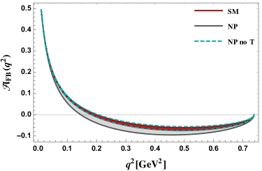
Figure 6: $q^{2}$-dependent forward-backward lepton asymmetry in $B_{c}^{+}\to B_{s}^{*}\mu^{+}\nu_{\mu}$. The red band corresponds to SM, the gray band to the full Hamiltonian (1). The region obtained excluding the tensor operator $T$ is indicated by the dashed cyan lines.

The effects of the new operators can also be observed in the coefficients $c_{0,1,2}$ defined in the expression [51, 52]

$$\frac{d{\cal B}(B_{c}^{+}\to B_{s}^{*}\,\mu^{+}\nu_{\mu})}{dq^{2}d\cos\theta}=c_{0}+c_{1}\cos\theta+c_{2}\cos^{2}\theta\,\,,$$ (21)

as shown in Fig. 7.

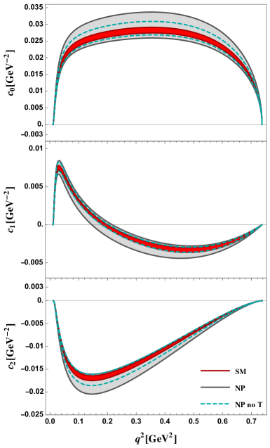
Figure 7: Coefficients $c_{0,1,2}$ in Eq. (21) for $B_{c}\to B^{*}_{s}\mu^{+}\nu_{\mu}$. The color codes are the same as in Fig. 6.

Interesting information is encoded in the correlations between the various observables in the decay modes to the pseudoscalar and vector meson. We analyze them in turn, neglecting the common FF uncertainties, considering the SM, each NP operator and all operators together. Since the scalar and pseudoscalar operators have a minor impact on the results, we do not discuss them individually.

Figure 8: Correlation between the branching fractions ${\cal B}(B_{c}^{+}\to B_{s}\mu^{+}\nu_{\mu}$) and ${\cal B}(B_{c}^{+}\to B_{s}^{*}\mu^{+}\nu_{\mu}$) in SM (black dot) and for the NP operators in Eq. (1). The regions labeled $VR$, $V$, $R$ and $T$ are obtained varying separately the coefficients of the corresponding operators in their quoted ranges. The NP-All region refers to the full set of operators in (1).

Fig. 8 shows the correlation between the branching fractions of the pseudoscalar and vector modes ${\cal B}(B_{c}^{+}\to B_{s}\,\mu^{+}\nu_{\mu})$ and ${\cal B}(B_{c}^{+}\to B_{s}^{*}\,\mu^{+}\nu_{\mu})$. The SM point corresponds to the central values in Eqs. (15) and (19). When all NP operators are considered the enlarged (pink) region is obtained. Anticorrelation between the branching fractions is found when the $R$ operator is considered. Increasing $\epsilon_{V}^{\mu}$ produces a positive correlation between the two observables. The tensor operator $T$ can allow a reduction of ${\cal B}(B_{c}^{+}\to B_{s}^{*}\,\mu^{+}\nu_{\mu})$ with respect to SM. Structured patterns are found in the correlations of the branching fractions ${\cal B}(B_{c}^{+}\to B_{s}\,\mu^{+}\nu_{\mu})$ and ${\cal B}(B_{c}^{+}\to B_{s}^{*}\,\mu^{+}\nu_{\mu})$ with the integrated FB lepton asymmetry in the $B^{*}_{s}$ mode

$$A_{FB}=\int_{q^{2}_{min}}^{q^{2}_{max}}dq^{2}\,{\cal A_{FB}}(q^{2})\,,$$ (22)

as shown in Fig. 9. Varying the $R$ and $V$ coefficients produces anticorrelations in case of the $B_{s}$ channel, same sign correlation in case of $B_{s}^{*}$. The tensor operator results in a mild anticorrelation in the $B_{s}^{*}$ case. The combined analysis of all observables can allow to isolate the signature of the different NP operators.

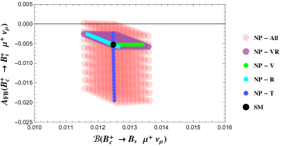
Figure 9: Correlations between the integrated forward-backward lepton asymmetry $A_{FB}$ in $B_{c}^{+}\to B_{s}^{*}\mu^{+}\nu_{\mu}$, defined in Eq. (22), with ${\cal B}(B_{c}^{+}\to B_{s}\,\mu^{+}\nu_{\mu})$ (top) and ${\cal B}(B_{c}^{+}\to B_{s}^{*}\mu^{+}\nu_{\mu})$ (bottom panel). The color codes are the same as in Fig. 8.

V.2 $B_{c}^{+}\to B_{d}\ell^{+}\nu_{\ell}$ and $B_{c}^{+}\to B_{d}^{*}(\to B_{d}\gamma)\ell^{+}\nu_{\ell}$

The $c\to d$ semileptonic $B_{c}$ modes also give access to relevant information. The SM expectations

$${\cal B}(B_{c}^{+}\to B_{d}\,\mu^{+}\nu_{\mu}) = 8.3\,(5)\times 10^{-4}\,\left(\frac{|V_{cd}|}{0.221}\right)^{2}$$

$${\cal B}(B_{c}^{+}\to B_{d}\,e^{+}\nu_{e}) = 8.7\,(5)\times 10^{-4}\,\left(\frac{|V_{cd}|}{0.221}\right)^{2}\,\,\,\,\,\,\,\,\,\,$$ (23)

derive from the form factors in [8]. The quoted errors are only due to the FF uncertainty. The corresponding predictions for $B_{c}^{+}\to B_{d}^{*}\,\bar{\ell}\nu_{\ell}$ in SM are

$${\cal B}(B_{c}^{+}\to B_{d}^{*}\,\mu^{+}\nu_{\mu}) = 20\,(1)\times 10^{-4}\,\left(\frac{|V_{cd}|}{0.221}\right)^{2}$$

$${\cal B}(B_{c}^{+}\to B_{d}^{*}\,e^{+}\nu_{e}) = 21\,(1)\times 10^{-4}\,\left(\frac{|V_{cd}|}{0.221}\right)^{2}.\,\,\,\,\,\,\,\,\,$$ (24)

For the $\mu$ channel, the impact of the NP operators in the decay distributions is shown in Fig. 10. The spectra in SM are affected by a small FF uncertainty. Including the NP operators sizably enlarges the spectrum of the pseudoscalar mode. The forward-backward asymmetry Eq. (20) for the pseudoscalar mode shows deviations from the SM expectation mainly due to the tensor operator, Fig. 11.

Large effects are allowed in $B_{c}^{+}\to B_{d}^{*}(\to B_{d}\gamma)\ell^{+}\nu_{\ell}$: this is due to the contribution of the tensor operator, that overwhelms the other ones if the coefficient $\epsilon_{T}^{\mu}$ is varied in the parameter space bound in [16] using $D$ meson decays.

The distributions of longitudinally and transversely polarized $B_{d}^{*}$, Fig. 12, show that the tensor operator can sizably affect the transverse distribution. In SM the integrated width to longitudinal $B^{*}_{d}$ is larger than to the transverse one, as shown in Fig. 13. The tensor operator can reverse such a hierachy.

Also the $q^{2}$-dependent forward-backward lepton asymmetry shows this effect, as seen in Fig. 14. The inclusion of the tensor operator produces a zero for the ${\cal A_{FB}}$ distribution in the range $q_{0}^{2}\in[0.27\,{\rm GeV}^{2},\,q^{2}_{max}]$, while in the SM $q_{0}^{2}=0.188(1)$ GeV² is expected. The position of the zero of ${\cal A_{FB}}(q^{2})$ has a remarkable discriminating power of NP operators. The effects of the new operators on the coefficients defined in (21) are shown in Fig. 15.

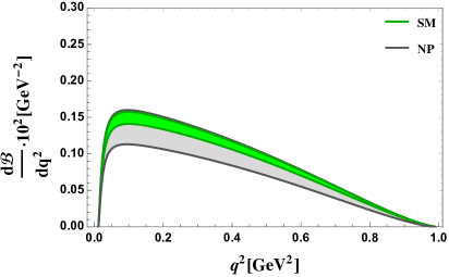
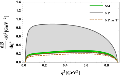
Figure 10: $q^{2}$ spectrum of the modes $B_{c}^{+}\to B_{d}\,\mu^{+}\nu_{\mu}$ (top) and $B_{c}^{+}\to B_{d}^{*}\,\mu^{+}\nu_{\mu}$ (bottom). The Standard Model results (green SM band) include the uncertainty on the form factors. The spectra for the full Hamiltonian in Eq. (1) are obtained varying the effective couplings in their quoted ranges (gray NP band). For $B_{c}^{+}\to B_{d}^{*}\,\mu^{+}\nu_{\mu}$ the spectrum obtained omitting the tensor operator $T$ is also shown (dashed orange lines).

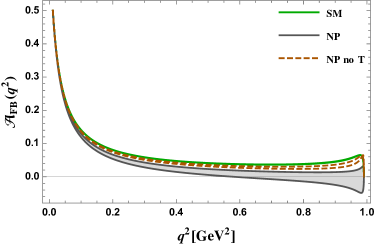
Figure 11: $q^{2}$-dependent forward-backward lepton asymmetry in $B_{c}^{+}\to B_{d}\,\mu^{+}\nu_{\mu}$. The green line corresponds to SM, the gray band is obtained for the Hamiltonian (1). The dashed orange lines are obtained excluding the tensor operator $T$.

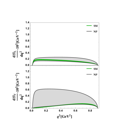
Figure 12: $q^{2}$ distribution of longitudinally (top) and transversely polarized $B_{d}^{*}$ (bottom) in $B_{c}^{+}\to B_{d}^{*}\,\mu^{+}\nu_{\mu}$. The color codes are as in Fig. 10.

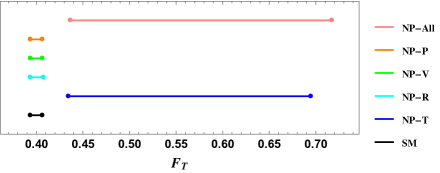
Figure 13: Fraction of transversely polarized $B_{d}^{*}$. The lines correspond to the SM, to the NP operators in Eq. (1) separately considered, and to the full set of NP operators.

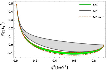
Figure 14: $q^{2}$-dependent forward-backward lepton asymmetry in $B_{c}^{+}\to B_{d}^{*}\,\mu^{+}\nu_{\mu}$. The green band corresponds to SM, the gray one is obtained for the Hamiltonian (1). The region obtained excluding the tensor operator $T$ (dashed orange lines) is also displayed.

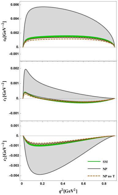
Figure 15: Coefficients $c_{0,1,2}$ in Eq. (21) for $B_{c}\to B^{*}_{d}\mu^{+}\nu_{\mu}$. The color codes are as in Fig. 14.

The correlation plots in Figs. 16 and 17 give access to other information. The branching factions ${\cal B}(B_{c}^{+}\to B_{d}^{*}\,\mu^{+}\nu_{\mu})$ and ${\cal B}(B_{c}^{+}\to B_{d}\,\mu^{+}\nu_{\mu})$ are sizably affected by the NP contributions. The $R$ operator anti-correlates the decay widths of the pseudoscalar and vector modes, while the $V$ contribution results in a positive correlation. In particular, ${\cal B}(B_{c}^{+}\to B_{d}^{*}\,\mu^{+}\nu_{\mu})$ increases with respect to SM if $R$ is included, and decreases considering only $V$. However, the main effect is due to the tensor operator that strongly enhances ${\cal B}(B_{c}^{+}\to B_{d}\,\mu^{+}\nu_{\mu})$ if its coefficient is varied in the range quoted in [16]. Such a macroscopic effect on the one hand requires to further scrutinize the bounds from the $D$ meson decays, on the other hand shows the relevance of the $B_{c}$ modes in the search of BSM signals. This is confirmed by the correlations between the integrated forward-backward lepton asymmetry $A_{FB}$ and the branching fractions of the pseudoscalar and vector modes. As shown in Fig. 17, the integrated $A_{FB}$, that in SM is predicted to be negative, is anti-correlated with ${\cal B}(B_{c}^{+}\to B_{d}\,\mu^{+}\nu_{\mu})$ mainly due to the tensor operator. $A_{FB}$ can become positive in the allowed range for the coefficient of such an operator, an interesting experimental signature. On the other hand, $A_{FB}$ and ${\cal B}(B_{c}^{+}\to B_{d}^{*}\,\mu^{+}\nu_{\mu})$ are positively correlated, and the enhancement of the branching fraction closely follows the enhancement of $A_{FB}$ obtained varying the coefficient of the tensor operator.

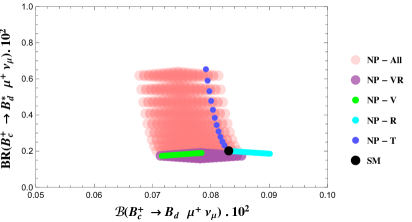
Figure 16: Correlation between the branching fractions ${\cal B}(B_{c}^{+}\to B_{d}\mu^{+}\nu_{\mu}$) and ${\cal B}(B_{c}^{+}\to B_{d}^{*}\mu^{+}\nu_{\mu}$) in SM (black dot) and considering the NP operators in Eq. (1). The regions labeled $VR$, $V$, $R$ and $T$ are obtained varying separately the coefficients of the corresponding operators in their quoted ranges. The NP-All region refers to the full set of operators in (1).

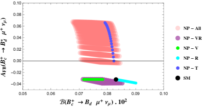
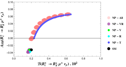
Figure 17: Correlations between the integrated forward-backward lepton asymmetry $A_{FB}$ in $B_{c}^{+}\to B_{d}^{*}\mu^{+}\nu_{\mu}$, defined in Eq. (22), with ${\cal B}(B_{c}^{+}\to B_{d}\,\mu^{+}\nu_{\mu})$ (top) and ${\cal B}(B_{c}^{+}\to B_{d}^{*}\mu^{+}\nu_{\mu})$ (bottom panel). The color codes are the same as in Fig. 16.

VI Conclusions

The semileptonic $B_{c}$ decays induced by the $c\to s,d$ transitions play an interesting role in SM and in the search of BSM effects analogous to the ones emerging in $B$ decays. The heavy quark spin symmetry has allowed to analyze the full phenomenology of such decays using two nonperturbative form factors obtained by lattice QCD. The assessment of the role of the symmetry-breaking terms requires additional nonperturbative information, namely some other form factor in few points of the kinematical range. We have studied several significant observables in these decay modes, together with the effects and their correlations of the SM extension involving dimension-6 operators and left-handed neutrinos.

On the basis of the available information on semileptonic $D$ decays we have found that sizable deviations from SM are allowed in $B_{c}^{+}\to B_{d}^{*}\,\mu^{+}\nu_{\mu}$. Of particular interest are the correlations of the effects of the NP operators in the various observables, that can be used to pin-down the single contributions. For example, the branching fractions of the pseudoscalar and vector modes are positively or negatively correlated if the $R$ or $V$ contributions are considered. Other correlations involve the integrated FB lepton asymmetry, in particular the effect of the tensor operator in the $B_{c}^{+}\to B_{d}^{*}\,\mu^{+}\nu_{\mu}$ mode correlated to the branching fraction. The position of the zero in the FB lepton distribution, as well as the fraction of longitudinally vs transversely polarized final vector mesons constitute other observables worth to measure.

VII Acknowledgements

We thank D. Bečirević, F. Jaffredo, A. Peñuelas and O. Sumensari for communications about Ref. [16]. This study has been carried out within the INFN project (Iniziativa Specifica) QFT-HEP.

Appendix A Hadronic matrix elements and form factors in SM and NP

We use the standard parametrization of the hadronic $B_{c}\to P,V$ matrix elements in terms of form factors, with $P$ a pseudoscalar and $V$ a vector meson. The $B_{c}\to P$ matrix elements of the vector $\bar{q}\gamma_{\mu}Q$ current, of the scalar density $\bar{q}Q$, and of the tensor $\bar{q}\sigma_{\mu\nu}Q$ and $\bar{q}\sigma_{\mu\nu}\gamma_{5}Q$ currents are parametrized as:

$$\langle P(p^{\prime})|{\bar{q}}\gamma_{\mu}Q|{B_{c}}(p)\rangle=$$

$$\quad\quad f_{+}^{B_{c}\to P}(q^{2})\Big{(}p_{\mu}+p_{\mu}^{\prime}-\frac{m_{B_{c}}^{2}-m_{P}^{2}}{q^{2}}q_{\mu}\Big{)}$$

$$\quad\quad+\,f_{0}^{B_{c}\to P}(q^{2})\frac{m_{B_{c}}^{2}-m_{P}^{2}}{q^{2}}q_{\mu}\,\,,$$

$$\langle P(p^{\prime})|{\bar{q}}Q|{B_{c}}(p)\rangle=f_{S}^{B_{c}\to P}(q^{2})\,\,,$$ (A.1)

$$\langle P(p^{\prime})|{\bar{q}}\sigma_{\mu\nu}Q|B_{c}(p)\rangle=-i\frac{2f_{T}^{B_{c}\to P}(q^{2})}{m_{B_{c}}+m_{P}}\big{(}p_{\mu}p_{\nu}^{\prime}-p_{\nu}p^{\prime}_{\mu}\big{)}\,\,,$$

$$\langle P(p^{\prime})|{\bar{q}}\sigma_{\mu\nu}\gamma_{5}Q|{B_{c}}(p)\rangle=-\frac{2f_{T}^{B_{c}\to P}(q^{2})}{m_{B_{c}}+m_{P}}\epsilon_{\mu\nu\alpha\beta}\,p^{\alpha}p^{\prime\beta},$$

with $\epsilon^{0123}=+1$. The condition $f_{+}^{B_{c}\to P}(0)=f_{0}^{B_{c}\to P}(0)$ holds. Moreover, one has $f_{S}^{B_{c}\to P}(q^{2})=\displaystyle\frac{m_{B_{c}}^{2}-m_{P}^{2}}{m_{Q}-m_{q}}f_{0}^{B_{c}\to P}(q^{2})$ in terms of the quark masses $m_{Q}$ and $m_{q}$.

The $B_{c}\to V$ matrix elements are parametrized as:

$$\langle V(p^{\prime},\epsilon)|{\bar{q}}\gamma_{\mu}Q|{B_{c}}(p)\rangle=-{2V^{B_{c}\to V}(q^{2})\over m_{B_{c}}+m_{V}}i\epsilon_{\mu\nu\alpha\beta}\epsilon^{*\nu}p^{\alpha}p^{\prime\beta},$$

$$\langle V(p^{\prime},\epsilon)|{\bar{q}}\gamma_{\mu}\gamma_{5}Q|{B_{c}}(p)\rangle=$$

$$(m_{B_{c}}+m_{V})\Big{(}\epsilon^{*}_{\mu}-{(\epsilon^{*}\cdot q)\over q^{2}}q_{\mu}\Big{)}A_{1}^{B_{c}\to V}(q^{2})$$

$$-{(\epsilon^{*}\cdot q)\over m_{B_{c}}+m_{V}}\Big{(}(p+p^{\prime})_{\mu}-{m_{B_{c}}^{2}-m_{V}^{2}\over q^{2}}q_{\mu}\Big{)}A_{2}^{B_{c}\to V}(q^{2})$$

$$+(\epsilon^{*}\cdot q){2m_{V}\over q^{2}}q_{\mu}A_{0}^{B_{c}\to V}(q^{2}),$$

$$\langle V(p^{\prime},\epsilon)|{\bar{q}}\gamma_{5}Q|{B_{c}}(p)\rangle=-\frac{2m_{V}}{m_{Q}+m_{q}}(\epsilon^{*}\cdot q)A_{0}^{B_{c}\to V}(q^{2}),$$

$$\langle V(p^{\prime},\epsilon)|{\bar{q}}\sigma_{\mu\nu}Q|{B_{c}}(p)\rangle=$$

$$\quad\quad T_{0}^{B_{c}\to V}(q^{2}){\epsilon^{*}\cdot q\over(m_{B_{c}}+m_{V})^{2}}\epsilon_{\mu\nu\alpha\beta}p^{\alpha}p^{\prime\beta}$$

$$\quad\quad+T_{1}^{B_{c}\to V}(q^{2})\epsilon_{\mu\nu\alpha\beta}p^{\alpha}\epsilon^{*\beta}$$

$$\quad\quad+T_{2}^{B_{c}\to V}(q^{2})\epsilon_{\mu\nu\alpha\beta}p^{\prime\alpha}\epsilon^{*\beta},$$ (A.2)

$$\langle V(p^{\prime},\epsilon)|{\bar{q}}\sigma_{\mu\nu}\gamma_{5}Q|{B_{c}}(p)\rangle=$$

$$\quad\quad i\,T_{0}^{B_{c}\to V}(q^{2}){\epsilon^{*}\cdot q\over(m_{B_{c}}+m_{V})^{2}}(p_{\mu}p^{\prime}_{\nu}-p_{\nu}p^{\prime}_{\mu})$$

$$\quad\quad+i\,T_{1}^{B_{c}\to V}(q^{2})(p_{\mu}\epsilon_{\nu}^{*}-\epsilon_{\mu}^{*}p_{\nu})$$

$$\quad\quad+i\,T_{2}^{B_{c}\to V}(q^{2})(p^{\prime}_{\mu}\epsilon_{\nu}^{*}-\epsilon_{\mu}^{*}p^{\prime}_{\nu}),$$

with the condition

$$A_{0}^{B_{c}\to V}(0) = \frac{m_{B_{c}}+m_{V}}{2m_{V}}A_{1}^{B_{c}\to V}(0)$$ (A.3)

$$- \frac{m_{B_{c}}-m_{V}}{2m_{V}}A_{2}^{B_{c}\to V}(0).\quad\quad\quad\quad$$

The relations among the form factors and the universal functions $\Omega_{1}(y)$ and $\Omega_{2}(y)$ are obtained using Eq. (12) [6]:

$$\langle P(v,k)|{\bar{q}}\gamma_{\mu}Q|{B_{c}}(v)\rangle=$$

$$\quad\quad 2\sqrt{m_{B_{c}}m_{P}}\Big{(}\Omega_{1}(y)\ v_{\mu}+a_{0}\Omega_{2}(y)\ k_{\mu}\Big{)},$$

$$\langle P(v,k)|{\bar{q}}Q|{B_{c}}(v)\rangle=2\sqrt{m_{B_{c}}m_{P}}\Big{(}\Omega_{1}(y)+a_{0}\Omega_{2}(y)\ v\cdot k\Big{)},$$

$$\langle P(v,k)|{\bar{q}}\sigma_{\mu\nu}Q|{B_{c}}(v)\rangle=$$

$$\quad\quad-2i\sqrt{m_{B_{c}}m_{P}}\ a_{0}\Omega_{2}(y)\Big{(}v_{\mu}k_{\nu}-v_{\nu}k_{\mu}\Big{)},$$ (A.4)

with $P=B_{s,d}$, $p=m_{B_{c}}v$, and $p^{\prime}=m_{P}v+k$,

$$\langle V(v,k,\epsilon)|{\bar{q}}\gamma_{\mu}Q|{B_{c}}(v)\rangle=$$

$$\,\,\,\,\,\,\,2i\sqrt{m_{B_{c}}m_{V}}\ a_{0}\Omega_{2}(y)\ \epsilon_{\mu\nu\alpha\beta}\epsilon^{*\nu}\ k^{\alpha}v^{\beta},$$

$$\langle V(v,k,\epsilon)|{\bar{q}}\gamma_{\mu}\gamma_{5}b|{B_{c}}(v)\rangle=2\sqrt{m_{B_{c}}m_{V}}$$

$$\,\,\,\,\,\,\,\Big{(}\epsilon^{*}_{\mu}\,\left(\Omega_{1}(y)+v\cdot k\ a_{0}\Omega_{2}(y)\right)$$

$$\,\,\,\,\,\,\,-(v_{\mu}-\frac{k_{\mu}}{m_{V}})\epsilon^{*}\cdot k\,a_{0}\Omega_{2}(y)\Big{)},$$

$$\langle V(v,k,\epsilon)|{\bar{q}}\sigma_{\mu\nu}Q|{B_{c}}(v)\rangle=-2\sqrt{m_{B_{c}}m_{V}}$$

$$\Big{(}\epsilon_{\mu\nu\alpha\beta}\epsilon^{*\alpha}v^{\beta}\Omega_{1}(y)+\epsilon_{\mu\nu\alpha\beta}\epsilon^{*\alpha}k^{\beta}a_{0}\Omega_{2}(y)\Big{)},\quad\quad\quad\quad$$ (A.5)

$$\langle V(v,k,\epsilon)|{\bar{q}}\sigma_{\mu\nu}\gamma_{5}Q|{B_{c}}(v)\rangle=2i\sqrt{m_{B_{c}}m_{V}}$$

$$\,\,\,\,\,\,\,\Big{(}\epsilon^{*}_{\nu}(v_{\mu}\Omega_{1}(y)+k_{\mu}a_{0}\Omega_{2}(y))$$

$$\,\,\,\,\,\,\,-\epsilon^{*}_{\mu}(v_{\nu}\Omega_{1}(y)+k_{\nu}a_{0}\Omega_{2}(y))\Big{)},$$

where $V=B^{*}_{s,d}$ and $y=1+\frac{v\cdot k}{m_{P,V}}$. Invoking the HQ spin symmetry and comparing the first equation in (A.1) to the corresponding one in (A.4), the form factors $\Omega_{1}$ and $\Omega_{2}$ are obtained from $f_{+}$ and $f_{0}$:

$$\Omega_{1} = \frac{m_{B_{c}}+m_{P}}{2q^{2}\sqrt{m_{B_{c}}m_{P}}}\Big{(}(m_{B_{c}}-m_{P})^{2}(f_{0}-f_{+})+q^{2}f_{+}\Big{)}$$

$$a_{0}\Omega_{2} = \frac{1}{2q^{2}\sqrt{m_{B_{c}}m_{P}}}\Big{(}(m_{B_{c}}^{2}-m_{P}^{2})(f_{+}-f_{0})+q^{2}f_{+}\Big{)}$$

with $q^{2}=m_{B_{c}}^{2}+m_{P}^{2}-2m_{B_{c}}m_{P}y$. These correspond to the results in Fig. 2. Further comparing (A.1) to (A.4), as well as (A.2) to (A.5), the relations of all form factors in terms of $\Omega_{1,2}$ can be derived. For $B_{c}\to P$ one has:

$$f_{+}^{B_{c}\to P} = \sqrt{\frac{m_{P}}{m_{B_{c}}}}\Big{(}\Omega_{1}+(m_{B_{c}}-m_{P})a_{0}\Omega_{2}\Big{)},$$

$$f_{0}^{B_{c}\to P} = \sqrt{\frac{m_{P}}{m_{B_{c}}}}\frac{1}{m_{B_{c}}^{2}-m_{P}^{2}}\Big{(}(m_{B_{c}}^{2}+q^{2}-m_{P}^{2})\Omega_{1}$$

$$+ (m_{B_{c}}+m_{P})((m_{B_{c}}-m_{P})^{2}-q^{2})a_{0}\Omega_{2}\Big{)},$$

$$f_{T}^{B_{c}\to P} = \sqrt{\frac{m_{P}}{m_{B_{c}}}}(m_{B_{c}}+m_{P})a_{0}\Omega_{2}\,\,.$$ (A.7)

For $B_{c}\to V$ one has:

$$V^{B_{c}\to V}=\sqrt{\frac{m_{V}}{m_{B_{c}}}}(m_{B_{c}}+m_{V})a_{0}\Omega_{2},$$

$$A_{0}^{B_{c}\to V}=$$

$$\quad\quad\frac{1}{2\sqrt{m_{B_{c}}m_{V}}}\Big{(}2m_{B_{c}}\Omega_{1}+(m_{B_{c}}^{2}-m_{V}^{2}+q^{2})a_{0}\Omega_{2}\Big{)},$$

$$A_{1}^{B_{c}\to V}=2\sqrt{m_{B_{c}}m_{V}}\frac{1}{m_{B_{c}}+m_{V}}\Omega_{1},$$

$$A_{2}^{B_{c}\to V}=-\sqrt{\frac{m_{V}}{m_{B_{c}}}}(m_{B_{c}}+m_{V})a_{0}\Omega_{2},$$ (A.8)

$$T_{1}^{B_{c}\to V}=2\sqrt{\frac{m_{V}}{m_{B_{c}}}}\Big{(}\Omega_{1}-m_{V}a_{0}\Omega_{2}\Big{)},$$

$$T_{2}^{B_{c}\to V}=2\sqrt{m_{B_{c}}m_{V}}a_{0}\Omega_{2},$$

$$T_{0}^{B_{c}\to V}=0.$$

Eqs.(A.7)-(A.8) are obtained for $v\cdot k=0$. Only $A_{0,1,2}$ are modified if this condition is not imposed, the other relations remain unaffected.

Appendix B Coefficient functions in the $B_{c}\to V(\to P\gamma)\,\bar{\ell}\nu_{\ell}$ full angular distribution

In Tables 2-6 we collect the functions $I_{i}$ in Eq. (3) for all operators in the Hamiltonian (1), with $H_{\pm},H_{0},H_{t}$ and $H_{\pm}^{NP},H_{L}^{NP}$ defined in Eqs. (7), (8).

Table 2: Angular coefficient functions in the decay distribution Eq. (3) for the Standard Model.

$i$	$I_{i}^{\rm SM}$
$I_{1s}$	$2m_{\ell}^{2}H_{t}^{2}+H_{0}^{2}(m_{\ell}^{2}+q^{2})$
$I_{1c}$	$\frac{1}{8}(H_{+}^{2}+H_{-}^{2})(m_{\ell}^{2}+3q^{2})$
$I_{2s}$	$H_{0}^{2}(m_{\ell}^{2}-q^{2})$
$I_{2c}$	$-\frac{1}{8}(H_{+}^{2}+H_{-}^{2})(m_{\ell}^{2}-q^{2})$
$I_{3}$	$H_{+}H_{-}(q^{2}-m_{\ell}^{2})$
$I_{4}$	$-\frac{1}{2}H_{0}(H_{+}+H_{-})(m_{\ell}^{2}-q^{2})$
$I_{5}$	$H_{t}(H_{+}+H_{-})m_{\ell}^{2}+H_{0}(H_{+}-H_{-})q^{2}$
$I_{6s}$	$-4H_{t}H_{0}m_{\ell}^{2}$
$I_{6c}$	$\frac{1}{2}(H_{+}^{2}-H_{-}^{2})q^{2}$
$I_{7,8,9}$	$0$

Table 3: Angular coefficient functions in NP with the operator ${\cal O}_{R}$ and interference SM-R terms. The functions $I_{i}^{\rm R}$ are obtained from the corresponding SM functions replacing $H_{+}\leftrightarrow H_{-}$.

$i$	$I_{i}^{\rm R}$	$I_{i}^{\rm INT,R}$
$I_{1s}$	$2m_{\ell}^{2}H_{t}^{2}+H_{0}^{2}(m_{\ell}^{2}+q^{2})$	$-2m_{\ell}^{2}H_{t}^{2}-H_{0}^{2}(m_{\ell}^{2}+q^{2})$
$I_{1c}$	$\frac{1}{8}(H_{+}^{2}+H_{-}^{2})(m_{\ell}^{2}+3q^{2})$	$-\frac{1}{4}H_{+}H_{-}(m_{\ell}^{2}+3q^{2})$
$I_{2s}$	$H_{0}^{2}(m_{\ell}^{2}-q^{2})$	$-H_{0}^{2}(m_{\ell}^{2}-q^{2})$
$I_{2c}$	$-\frac{1}{8}(H_{+}^{2}+H_{-}^{2})(m_{\ell}^{2}-q^{2})$	$\frac{1}{4}H_{+}H_{-}(m_{\ell}^{2}-q^{2})$
$I_{3}$	$H_{+}H_{-}(q^{2}-m_{\ell}^{2})$	$\frac{1}{2}(H_{+}^{2}+H_{-}^{2})(m_{\ell}^{2}-q^{2})$
$I_{4}$	$-\frac{1}{2}H_{0}(H_{+}+H_{-})(m_{\ell}^{2}-q^{2})$	$\frac{1}{2}H_{0}(H_{+}+H_{-})(m_{\ell}^{2}-q^{2})$
$I_{5}$	$H_{t}(H_{+}+H_{-})m_{\ell}^{2}$	$-H_{t}(H_{+}+H_{-})m_{\ell}^{2}$
	$-H_{0}(H_{+}-H_{-})q^{2}$
$I_{6s}$	$-4H_{t}H_{0}m_{\ell}^{2}$	$4H_{t}H_{0}m_{\ell}^{2}$
$I_{6c}$	$-\frac{1}{2}(H_{+}^{2}-H_{-}^{2})q^{2}$	0
$I_{7}$	$0$	$-H_{t}(H_{+}-H_{-})m_{\ell}^{2}$
$I_{8}$	$0$	$\frac{1}{2}H_{0}(H_{+}-H_{-})(m_{\ell}^{2}-q^{2})$
$I_{9}$	$0$	$\frac{1}{2}(H_{+}^{2}-H_{-}^{2})(m_{\ell}^{2}-q^{2})$

Table 4: Angular coefficient functions for NP with the pseudoscalar P operator, and interference SM-P terms.

$i$	$I_{i}^{\textsc{NP},P}$	$I_{i}^{\textsc{INT},P}$
$I_{1s}$	$2H_{t}^{2}\frac{q^{4}}{(m_{Q}+m_{q})^{2}}$	$2H_{t}^{2}\frac{m_{\ell}q^{2}}{m_{Q}+m_{q}}$
$I_{1c,2s,2c,6c,3,4,8,9}$	$0$	$0$
$I_{5}$	$0$	$H_{t}(H_{+}+H_{-})\frac{m_{\ell}q^{2}}{2(m_{Q}+m_{q})}$
$I_{6s}$	$0$	$-2H_{t}H_{0}\frac{m_{\ell}q^{2}}{m_{Q}+m_{q}}$
$I_{7}$	$0$	$H_{t}(H_{+}-H_{-})\frac{m_{\ell}q^{2}}{2(m_{Q}+m_{q})}$

Table 5: Angular coefficient functions for NP with the tensor T operator and interference SM-T terms.

$i$	$I_{i}^{\rm NP,T}$	$I_{i}^{\rm INT,T}$
$I_{1s}$	$\frac{1}{16}(H_{L}^{\textsc{NP}})^{2}(m_{\ell}^{2}+q^{2})$	$-\frac{1}{2}H_{L}^{\textsc{NP}}H_{0}m_{\ell}\sqrt{q^{2}}$
$I_{1c}$	$\frac{1}{2}[(H_{+}^{\textsc{NP}})^{2}+(H_{-}^{\textsc{NP}})^{2}](3m_{\ell}^{2}+q^{2})$	$-(H_{+}^{\textsc{NP}}H_{+}+H_{-}^{\textsc{NP}}H_{-})m_{\ell}\sqrt{q^{2}}$
$I_{2s}$	$\frac{1}{16}(H_{L}^{\textsc{NP}})^{2}(q^{2}-m_{\ell}^{2})$	$0$
$I_{2c}$	$\frac{1}{2}[(H_{+}^{\textsc{NP}})^{2}+(H_{-}^{\textsc{NP}})^{2}](m_{\ell}^{2}-q^{2})$	$0$
$I_{3}$	$-4H_{+}^{\textsc{NP}}H_{-}^{\textsc{NP}}(q^{2}-m_{\ell}^{2})$	$0$
$I_{4}$	$-\frac{1}{4}H_{L}^{\textsc{NP}}(H_{+}^{\textsc{NP}}+H_{-}^{\textsc{NP}})(q^{2}-m_{\ell}^{2})$	$0$
$I_{5}$	$\frac{1}{2}H_{L}^{\textsc{NP}}(H_{+}^{\textsc{NP}}-H_{-}^{\textsc{NP}})m_{\ell}^{2}$	$-\frac{1}{8}[H_{L}^{\textsc{NP}}(H_{+}-H_{-})+8H_{+}^{\textsc{NP}}(H_{t}+H_{0})+8H_{-}^{\textsc{NP}}(H_{t}-H_{0})]m_{\ell}\sqrt{q^{2}}$
$I_{6s}$	$0$	$\frac{1}{2}H_{L}^{\textsc{NP}}H_{t}m_{\ell}\sqrt{q^{2}}$
$I_{6c}$	$2[(H_{+}^{\textsc{NP}})^{2}-(H_{-}^{\textsc{NP}})^{2}]m_{\ell}^{2}$	$-(H_{+}^{\textsc{NP}}H_{+}-H_{-}^{\textsc{NP}}H_{-})m_{\ell}\sqrt{q^{2}}$
$I_{7}$	$0$	$-\frac{1}{8}[H_{L}^{\textsc{NP}}(H_{+}+H_{-})-8H_{+}^{\textsc{NP}}(H_{t}+H_{0})+8H_{-}^{\textsc{NP}}(H_{t}-H_{0})]m_{\ell}\sqrt{q^{2}}$
$I_{8,9}$	$0$	$0$

Table 6: P-R, R-T and P-T interference terms in the angular coefficient functions.

$i$	$I_{i}^{\textsc{INT},PR}$	$I_{i}^{\textsc{INT},RT}$	$I_{i}^{INT,PT}$
$I_{1s}$	$-2H_{t}^{2}\frac{m_{\ell}q^{2}}{(m_{b}+m_{q})}$	$\frac{1}{2}H_{0}H_{L}^{\textsc{NP}}m_{\ell}\sqrt{q^{2}}$	$0$
$I_{1c}$	$0$	$(H_{+}^{NP}H_{-}+H_{-}^{NP}H_{+})m_{\ell}\sqrt{q^{2}}$	$0$
$I_{2s,2c,3,4,8,9}$	$0$	$0$	$0$
$I_{5}$	$-H_{t}(H_{+}+H_{-})\frac{m_{\ell}q^{2}}{2(m_{Q}+m_{q})}$	$\frac{1}{8}[H_{L}^{\textsc{NP}}(H_{-}-H_{+})+8H_{+}^{\textsc{NP}}(H_{t}+H_{0})$	$-H_{t}(H_{+}^{NP}+H_{-}^{NP})\frac{(q^{2})^{3/2}}{m_{Q}+m_{q}}$
		$\qquad\qquad+8H_{-}^{\textsc{NP}}(H_{t}-H_{0})]m_{\ell}\sqrt{q^{2}}$
$I_{6s}$	$2H_{t}H_{0}\frac{m_{\ell}q^{2}}{m_{Q}+m_{q}}$	$-\frac{1}{2}H_{t}\,H_{L}^{NP}m_{\ell}\sqrt{q^{2}}$	$H_{t}\,H_{L}^{NP}\frac{(q^{2})^{3/2}}{2(m_{Q}+m_{q})}$
$I_{6c}$	$0$	$(H_{+}^{NP}H_{-}-H_{-}^{NP}H_{+})m_{\ell}\sqrt{q^{2}}$	$0$
$I_{7}$	$H_{t}(H_{+}-H_{-})\frac{m_{\ell}q^{2}}{2(m_{Q}+m_{q})}$	$-\frac{1}{8}[H_{L}^{\textsc{NP}}(H_{-}+H_{+})-8H_{+}^{\textsc{NP}}(H_{t}+H_{0})$	$-H_{t}(H_{+}^{NP}-H_{-}^{NP})\frac{(q^{2})^{3/2}}{m_{Q}+m_{q}}$
		$\qquad\qquad+8H_{-}^{\textsc{NP}}(H_{t}-H_{0})]m_{\ell}\sqrt{q^{2}}$