Towards Certifying Robustness
using Neural Networks with -dist Neurons
Abstract
It is well-known that standard neural networks, even with a high classification accuracy, are vulnerable to small -norm bounded adversarial perturbations. Although many attempts have been made, most previous works either can only provide empirical verification of the defense to a particular attack method, or can only develop a certified guarantee of the model robustness in limited scenarios. In this paper, we seek for a new approach to develop a theoretically principled neural network that inherently resists perturbations. In particular, we design a novel neuron that uses -distance as its basic operation (which we call -dist neuron), and show that any neural network constructed with -dist neurons (called -dist net) is naturally a 1-Lipschitz function with respect to -norm. This directly provides a rigorous guarantee of the certified robustness based on the margin of prediction outputs. We then prove that such networks have enough expressive power to approximate any 1-Lipschitz function with robust generalization guarantee. We further provide a holistic training strategy that can greatly alleviate optimization difficulties. Experimental results show that using -dist nets as basic building blocks, we consistently achieve state-of-the-art performance on commonly used datasets: 93.09% certified accuracy on MNIST (), 35.42% on CIFAR-10 () and 16.31% on TinyImageNet ().
1 Introduction
Modern neural networks are usually sensitive to small, adversarially chosen perturbations to the inputs (Szegedy et al., 2013; Biggio et al., 2013). Given an image that is correctly classified by a neural network, a malicious attacker may find a small adversarial perturbation such that the perturbed image , though visually indistinguishable from the original image, is assigned to a wrong class with high confidence by the network. Such vulnerability creates security concerns in many real-world applications.
Developing a model that can resist small perturbations has been extensively studied in the literature. Adversarial training methods (Szegedy et al., 2013; Goodfellow et al., 2015; Madry et al., 2017; Zhang et al., 2019; Ding et al., 2020) first generate on-the-fly adversarial examples of the inputs, then update model parameters using these perturbed samples together with the original labels. While such approaches can achieve decent empirical robustness, the evaluation is restricted to a particular (class of) attack method, and there are no formal guarantees whether the resulting model is robust against other attacks (Athalye et al., 2018; Tramer et al., 2020; Tjeng et al., 2019).
Another line of algorithms train provably robust models for standard networks by maximizing the certified radius provided by robust certification methods, typically using linear relaxation (Wong & Kolter, 2018; Weng et al., 2018; Mirman et al., 2018; Zhang et al., 2018; Wang et al., 2018; Singh et al., 2018), semidefinite relaxation (Raghunathan et al., 2018; Dvijotham et al., 2020), interval bound relaxation (Mirman et al., 2018; Gowal et al., 2018) or their combinations (Zhang et al., 2020b). However, most of these methods are sophisticated to implement and computationally expensive. Besides these approaches, Cohen et al. (2019a); Salman et al. (2019); Zhai et al. (2020) study the certified guarantee on perturbations for Gaussian smoothed classifiers. However, recent works suggest that such methods are hard to extend to the -perturbation scenario if the input dimension is large.
In this work, we propose a new approach by introducing a novel type of neural network that naturally resists local adversarial attacks, and can be easily certified under perturbation. In particular, we propose a novel neuron called -dist neuron. Unlike the standard neuron design that uses a linear transformation followed by a non-linear activation, the -dist neuron is purely based on computing the -distance between the inputs and the parameters. It is straightforward to see that such a neuron is 1-Lipschitz with respect to -norm, and the neural networks constructed with -dist neurons (called -dist nets) enjoy the same property. Based on such a property, we can efficiently obtain the certified robustness for any -dist net using the margin of the prediction outputs.
Theoretically, we investigate the expressive power of -dist nets and their robust generalization ability. We first prove a Lipschitz-universal approximation theorem which shows that -dist nets can approximate any 1-Lipschitz function (with respect to -norm) arbitrarily well. We then give upper bounds of robust test error, which would be small if the -dist net learns a large margin classifier on the training data. These results demonstrate the excellent expressivity and generalization ability of the -dist net function class.
While -dist nets have nice theoretical guarantees, training such a network is still challenging. For example, the gradient of the parameters for -norm distance is sparse, which makes the optimization difficult. In addition, we find that commonly used tricks and techniques in conventional network training cannot be taken for granted for this fundamentally different architecture. We address these challenges by proposing a holistic strategy for -dist net training. Specifically, we show how to initialize the model parameters, apply proper normalization, design suitable weight decay mechanism, and overcome the sparse gradient problem via smoothed approximated gradients. Using the above methods, training an -dist net is just as easy as training a standard network without any adversarial training, even though the resulting model is already provably robust.
Furthermore, the -dist net has wide adaptability by serving as a robust feature extractor and combining itself with conventional networks for practical applications. After building a simple 2-layer perceptron on top of an -dist net, we show that the model allows fast training and certification, and consistently achieves state-of-the-art certified robustness on a wide range of classification tasks. Concretely, we reach 93.09% certified accuracy on MNIST under perturbation , 79.23% on FashionMNIST under , 35.42% on CIFAR-10 under , and 16.31% on TinyImageNet under . As a comparison, these results outperform the previous best-known results (Xu et al., 2020a), in which they achieve 33.38% certified accuracy on CIFAR-10 dataset, and achieve 15.86% certified accuracy on TinyImageNet using a WideResNet model which is 33 times larger than the -dist net.
Our contributions are summarized as follows:
-
•
We propose a novel neural network using -dist neurons, called -dist net. We show that any -dist net is 1-Lipschitz with respect to -norm, which directly guarantees the certified robustness (Section 3).
-
•
In the theoretical part, we prove that -dist nets can approximate any 1-Lipschitz function with respect to -norm. We also prove that -dist nets have a good robust generalization ability (Section 4).
-
•
In the algorithmic part, we provide a holistic training strategy for -dist nets, including parameter initialization, normalization, weight decay and smoothed approximated gradients (Section 5).
-
•
We show how to combine -dist nets with standard networks and obtain robust models more effectively (Section 6). Experimental results show that we can consistently achieve state-of-the-art certified accuracy on MNIST, Fashion-MNIST, CIFAR-10 and TinyImageNet dataset (Section 7).
-
•
Finally, we provide all the implementation details and codes at https://github.com/zbh2047/L_inf-dist-net.
2 Related Work
Robust Training Approaches.
Adversarial training is the most successful method against adversarial attacks. By adding adversarial examples to the training set on the fly, adversarial training methods (Szegedy et al., 2013; Goodfellow et al., 2015; Madry et al., 2017; Huang et al., 2015; Zhang et al., 2019; Wong et al., 2020; Ding et al., 2020) can significantly improve the robustness of conventional neural networks. However, all the methods above are evaluated according to the empirical robust accuracy against pre-defined adversarial attack algorithms, such as projected gradient decent. These methods cannot guarantee whether the resulting model is also robust against other attacks.
Certified Robustness for Conventional Networks.
Many recent works focus on certifying the robustness of learned neural networks under any attack. These approaches are mainly based on bounding the certified radius layer by layer using some convex relaxation methods (Wong & Kolter, 2018; Wong et al., 2018; Weng et al., 2018; Mirman et al., 2018; Dvijotham et al., 2018b; Zhang et al., 2018; Wang et al., 2018; Singh et al., 2018; Xiao et al., 2019; Balunovic & Vechev, 2020; Raghunathan et al., 2018; Dvijotham et al., 2020). However, such approaches are usually complicated, computationally expensive and have difficulties in applying to deep and large models. To overcome these drawbacks, Mirman et al. (2018); Gowal et al. (2018) considered interval bound propagation (IBP), a special form of convex relaxation which is much simpler and computationally cheaper. However, the produced bound is loose which results in unstable training. Zhang et al. (2020b); Xu et al. (2020a) took a further step to combine IBP with linear relaxation to make the bound tighter, which achieves current state-of-the-art performance. Fundamentally different from all these approaches that target to certify conventional networks, we proposed a novel network that provides robustness guarantee by its nature.
Certified Robustness for Smoothed Classifiers.
Randomized smoothing can provide a (probabilistic) certified robustness guarantee for general models. Lecuyer et al. (2018); Li et al. (2018); Cohen et al. (2019a); Salman et al. (2019); Zhai et al. (2020); Zhang et al. (2020a) showed that if a Gaussian random noise is added to the input, a certified guarantee on small perturbation can be computed for Gaussian smoothed classifiers. However, Yang et al. (2020); Blum et al. (2020); Kumar et al. (2020) showed that randomized smoothing cannot achieve nontrivial certified accuracy against larger than radius for perturbations, where is the input dimension. Therefore it cannot provide meaningful results for a relatively large perturbation due to the curse of dimensionality.
Lipschitz Networks.
Another line of approaches sought to bound the global Lipschitz constant of the neural network. Lipschitz networks can be very useful in certifying adversarial robustness (Tsuzuku et al., 2018), proving generalization bounds (Sokolić et al., 2017), or estimating Wasserstein distance (Arjovsky et al., 2017). Previous works trained Lipschitz ReLU networks by either directly constraining the spectral norm of each weight matrix to be less than one, or optimizing a loss constructed using the global Lipschitz constant which is upper bounded by these spectral norms (Cisse et al., 2017; Yoshida & Miyato, 2017; Gouk et al., 2018; Tsuzuku et al., 2018; Qian & Wegman, 2019). However, as pointed out by Huster et al. (2018) and Anil et al. (2019), such Lipschitz networks lack expressivity to some simple Lipschitz functions and the global Lipschitz bound is not tight. Recently, Anil et al. (2019) proposed a new Lipschitz network that is a Lipschitz-universal approximator. (Li et al., 2019) extended their work to convolutional architectures. However, the robustness performances are still not as good as other certification methods, and none of these methods can provide good certified results for robustness. In this work, we show the proposed -dist net is also a Lipschitz-universal approximator (under -norm), and the Lipschitz -dist net can substantially outperform other Lipschitz networks in term of certified accuracy.
-dist Neurons.
We notice that recently Chen et al. (2020); Xu et al. (2020b) proposed a new network called AdderNet, which leverages -norm operation to build the network for sake of efficient inference. Wang et al. (2019) also considered replacing dot-product neurons by -dist or -dist neurons in order to enhance the model’s non-linearity and expressivity. Although -dist net looks similar to these networks on the surface, they are designed for fundamentally different problems, and in fact -dist neurons (or -dist neurons) can not give any robust guarantee for norm-bounded perturbations (see Appendix C for more discussions).
3 -dist Network and its Robustness Guarantee
3.1 Preliminaries
Consider a standard classification task. Suppose we have an underlying data distribution over pairs of examples and corresponding labels where is the number of classes. Usually is unknown and we can only access a training set in which is i.i.d. drawn from . Let be the classifier of interest that maps any to . We call an adversarial example of to classifier if can correctly classify but assigns a different label to . In real practice, the most commonly used setting is to consider the attack under -bounded -norm constraint, i.e., satisfies , which is also called perturbations.
Our goal is to learn a model from that can resist attacks at over for any small perturbation. It relates to compute the radius of the largest ball centered at in which does not change its prediction. This radius is called the robust radius, which is defined as (Zhai et al., 2020; Zhang et al., 2019):
| (1) |
Unfortunately, exactly computing the robust radius of a classifier induced by a standard deep neural network is very difficult. For example, Katz et al. (2017) showed that calculating such radius for a DNN with ReLU activation is NP-hard. Researchers then seek to derive a tight lower bound of for general . Such lower bound is called certified radius and we denote it as . It follows that for any .
3.2 Networks with -dist Neurons
In this subsection, we propose a novel neuron called the -dist neuron, which is inherently robust with respect to -norm perturbations. Using these neurons as building blocks, we then show how to obtain robust neural networks dubbed -dist nets.
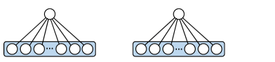
Denote as the input vector to a neuron. A standard neuron processes the input by first projecting to a scalar value using a linear transformation, then applying a non-linear activation function on it, i.e., with and as parameters and function being sigmoid or ReLU activation. Unlike the previous design paradigm, we introduce a new type of neuron using distance as the basic operation, called -dist neuron:
| (2) |
where is the parameter set (see Figure 1 for an illustration). From Eqn. 2 we can see that the -dist neuron is non-linear as it calculates the -distance between input and parameter with a bias term . As a result, there is no need to further apply a non-linear activation function.
Remark 3.1.
Conventional neurons use dot-product to represent the similarity between input and weight . Likewise, -distance is also a similarity measure. Note that -distance is always non-negative, and a smaller -distance indicates a stronger similarity.
Without loss of generality, we study the properties of multi-layer perceptron (MLP) networks constructed using -dist neurons. All theoretical results can be easily extended to other neural network architectures, such as convolutional networks. We use to denote the input vector of an MLP network. An MLP network using -dist neurons can be formally defined as follows.
Definition 3.2.
(-dist Net) Define an layer -dist net as follows. Assume the -th hidden layer contains hidden units. The network takes as input, and the -th unit in the -th hidden layer is computed by
| (3) | |||
where is the output of the -th layer.
For classification tasks, the dimension of the final outputs of an -dist net matches the number of categories, i.e., . Based on Remark 3.1, we use the negative of the final layer to be the outputs of the -dist net , i.e. and define the predictor . Similar to conventional networks, we can apply any standard loss function on the -dist net, such as the cross-entropy loss or hinge loss.
3.3 Lipschitz and Robustness Facts about -dist Nets
In this subsection, we will show that the -dist neurons and the neural networks constructed using them have nice theoretical properties in controlling the robustness of the model. We first show that -dist nets are 1-Lipschitz with respect to -norm, then derive the certified robustness of the model based on such property.
Definition 3.3.
(Lipschitz Function) A function is called -Lipschitz with respect to -norm , if for any , the following holds:
Fact 3.4.
Any -dist net is 1-Lipschitz with respect to -norm, i.e., for any , we have .
Proof.
It’s easy to check that every basic operation is 1-Lipschitz, and therefore the mapping from one layer to the next is 1-Lipschitz. Finally by composition we have for any , . ∎
Remark 3.5.
Fact 3.4 is only true when the basic neuron uses infinity-norm distance. For a network constructed using -dist neurons where (e.g. 2-norm), such network will not be 1-Lipschitz (even with respect to -norm) because the mapping from one layer to the next is not 1-Lipschitz.
Since is 1-Lipschitz with respect to -norm, if the perturbation over is rather small, the change of the output can be bounded and the prediction of the perturbed data will not change as long as , which directly bounds the certified radius.
Fact 3.6.
Given model defined above, and being correctly classified, we define as the difference between the largest and second-largest elements of . Then for any satisfying , we have that . In other words,
| (4) |
Proof.
Since is 1-Lipschitz, each element of can move at most when changes to , therefore the largest element will remain the same. ∎
Using this bound, we can certify the robustness of an -dist net of any size under -norm perturbations with little computational cost (only a forward pass). In contrast, existing certified methods may suffer from either poor scalability (methods based on linear relaxation) or curse of dimensionality (randomized smoothing).
4 Theoretical Properties of -dist Nets
The expressive power of a model family and its generalization are two central topics in machine learning. Since we have shown that -dist nets are 1-Lipschitz with respect to -norm, it’s natural to ask whether -dist nets can approximate any 1-Lipschitz function (with respect to -norm) and whether we can give generalization guarantee on the robust test error based on the Lipschitz property. In this section, we give affirmative answers to both questions. Without loss of generality, we consider binary classification problems and assume the output dimension is 1. All the omitted proofs in this section can be found in Appendix A.
4.1 Lipschitz-Universal Approximation of -dist Nets
It is well-known that the conventional network is a universal approximator, in that it can approximate any continuous function arbitrarily well (Cybenko, 1989). Similarly, in this section we will prove a Lipschitz-universal approximation theorem for -dist nets, formalized in the following:
Theorem 4.1.
For any 1-Lipschitz function (with respect to -norm) on a bounded domain and any , there exists an -dist net with width no more than , such that for all , we have .
We briefly present a proof sketch of Theorem 4.1. The proof has the same structure to Lu et al. (2017), who first proved such universal approximation theorem for width-bounded ReLU networks, by constructing a special network that approximates a target function by the sum of indicator functions of grid points, i.e. where . For -dist nets, such an approach cannot be directly applied as the summation will break the Lipschitz property. We employ a novel “max of pyramids” construction to overcome the issue. The key idea is to approximate the target function using the maximum of many “pyramid-like” basic 1-Lipschitz functions, i.e. . To represent such a function, we first show that the -dist neuron can express the following basic functions: , , and ; Then can be constructed using these functions as building blocks. Finally, we carefully design a computation pattern for a width-bounded -dist net to perform such max-reduction layer by layer.
4.2 Bounding Robust Test Error of -dist Nets
In this subsection, we give a generalization bound for the robust test error of -dist nets. Let be an instance-label couple where and and denote as the distribution of . For a function , we use as the classifier. The -robust test error of a classifier is defined as
Then can be upper bounded by the margin error on training data and the size of the network, as stated in the following theorem:
Theorem 4.2.
Let denote the set of all represented by an -dist net with width and depth . For every , with probability at least over the random drawing of samples, for all and we have that
| (5) | |||
Theorem 4.2 demonstrates that when a large margin classifier is found on training data, and the size of the -dist net is not too large, then with high probability, the model can generalize well in terms of adversarial robustness. Note that our bound does not depend on the input dimension, while previous generalization bounds for the general Lipschitz model class (i.e. Luxburg & Bousquet (2004)) suffer from the curse of dimensionality (Neyshabur et al., 2017).
5 Training -dist Nets
In this section we will focus on how to train an -dist net successfully. Motivated by the theoretical analysis in previous sections, it suffices to find a large margin solution on the training data. Therefore we can simply use the standard multi-class hinge loss to obtain a large training margin, similar to Anil et al. (2019). Since the loss is differentiable almost everywhere, any gradient-based optimization method can be used to train -dist nets.
However, we empirically find that the optimization is challenging and directly training the network usually fails to obtain a good performance. Moreover, conventional wisdom like batch normalization cannot be taken as a grant in the -dist net since it will hurt the model’s robustness. In the following we will dig into the optimization difficulties and provide a holistic training strategy to overcome them.
5.1 Normalization
One important difference between -dist nets and conventional networks is that for conventional networks, the output of a linear layer is unbiased (zero mean in expectation) under random initialization over parameters (Glorot & Bengio, 2010; He et al., 2015), while the output of an -dist neuron is biased (always being non-negative, assuming no bias term). Indeed, for a weight vector initialized using a standard Gaussian distribution, assume a zero input is fed into an -dist net, the expected output of the first layer can be approximated by . The output vector is then fed into subsequent layers, making the outputs in upper layers linearly increase.
Normalization is a useful way to control the scale of the layer’s outputs to a standard range. Batch Normalization (Ioffe & Szegedy, 2015), which shifts and scales feature values in each layer, is shown to be one of the most important components in training deep neural networks. However, if we directly apply batch normalization in -dist nets, the Lipschitz constant will change due to the scaling operation, and the robustness of the model cannot be guaranteed.
Fortunately, we find using the shift operation alone already helps the optimization. Therefore we apply the shift operation in all intermediate layers after calculating the distance. As a result, we remove the bias terms in the corresponding -dist neurons as they are redundant. We do not use normalization in the final layer. Similar to BatchNorm, we use the running mean during inference, which serves as additional bias terms in -dist neurons and does not affect the Lipschitz constant of the model. We do not use affine transformation, which is typically used in BatchNorm.
5.2 Smoothed Approximated Gradients
We find that training an -dist net from scratch is usually inefficient, and the optimization can easily be stuck at some bad solution. One important reason is that the gradients of the -dist operation (i.e., and ) are very sparse which typically contain only one non-zero element. In practice, we observe that there are less than 1% parameters updated in an epoch if we directly train the -dist net using SGD/Adam from random initialization.
To improve the optimization, we relax the -dist neuron by using the -dist neuron for the whole network to get an approximate and non-sparse gradient of the model parameters. During training, we set to be a small value in the beginning and increase it in each iteration until it approaches infinity. For the last few epochs, we set to infinity and train the model to the end. Empirically, using smoothed approximated gradients significantly boosts the performance, as will be shown in Section 7.3.
5.3 Parameter Initialization
We find that there are still optimization difficulties in training deep models using normalization and the smoothed gradient method. In particular, we find that a deeper model performs worse than its shallow counterpart in term of training accuracy (see Appendix E), a phenomenon similar to He et al. (2016). To fix the problem, He et al. (2016) proposed ResNet architecture by modifying the network using identity mapping as skip connections. According to Proposition A.2 (see Appendix A), an -dist layer can also perform identity mapping by assigning proper weights and biases at initialization, and a deeper -dist net then can act as a shallow one by these identity mappings.
Given such findings, we can directly construct identity mappings at initialization. Concretely, for an -dist layer with the same input-output dimension, we first initialize the weights randomly from a standard Gaussian distribution as common, then modify the diagonal elements (i.e. in Definition 3.2) to be a large negative number . Throughout all experiments, we set . We do not need the bias in -dist neurons after applying mean shift normalization, and the running mean automatically makes an identity mapping.
5.4 Weight Decay
Weight decay is a commonly used trick in training deep neural networks. It is equivalent to adding an regularization term to the loss function. However, we empirically found that using weight decay in the -dist net gives inferior performance (see Section 7.3). The problem might be the incompatibility of weight decay ( regularization) with -norm used in -dist nets, as we will explain below.
Conventional networks use dot-product as the basic operation, therefore an -norm constraint on the weight vectors directly controls the scale of the output magnitude. However, it is straightforward to see that the -norm of the weight vector does not correspond to the output scale of the distance operation. A more reasonable choice is to use -norm regularization instead of -norm. In fact, we have , analogous to .
For general -dist neurons during training, we can use -norm regularization analogously. By taking derivative with respect to the weight , we derive the corresponding weight decay formula:
| (6) |
where is the weight decay coefficient. Note that Eqn. 6 reduces to commonly used weight decay if . When , the weight decay tends to take effects only on the element with the largest absolute value.
6 Certified Robustness by Using -dist Nets as Robust Feature Extractors
We have shown that the -dist net is globally Lipschitz in the sense that the function is 1-Lipschitz everywhere over the input space. This constraint is pretty strong when we only require function’s Lipschitzness on a specific manifold, such as real image data manifold. To make the model more flexible and fit the practical tasks better, we can build a lightweight conventional network on top of an -dist net. The -dist net will serve as a robust feature extractor, and the lightweight network (a shallow MLP in our experiments) will focus on task-specific goals, such as classification. We denote the composite network as .
We first show how to certify the robustness for the composite network . Given any input , consider a perturbation set , where is the pre-defined perturbation level. If predicts the correct label for all , we can guarantee robustness of the network for input . Since is 1-Lipschitz with respect to -norm, we have by definition. Based on this property, to guarantee robustness of the network for input , it suffices to check whether for all , predicts the correct label . This is equivalent to certifying the robustness for a conventional network given input , which can be calculated using any previous certification method such as convex relaxation. We describe one of the simplest convex relaxation method named IBP (Gowal et al., 2018) in Appendix B, which is used in our experiments. Other more advanced approaches such as CROWN-IBP (Zhang et al., 2020b; Xu et al., 2020a) can also be considered.
After obtaining the bound, we can set it as the training objective function to train the neural network parameters, similar to Gowal et al. (2018); Zhang et al. (2020b). All calculations are differentiable, and gradient-based optimization methods can be applied. Note that since and have entirely different architectures, we apply the training strategy introduced in Section 5 to the -dist net only. More details will be presented in Section 7.1.
7 Experiments & Results
In this section, we conduct extensive experiments for the proposed network. We train our models on four popular benchmark datasets: MNIST, Fashion-MNIST, CIFAR-10 and TinyImagenet.
7.1 Experimental Setting
Model details.
We mainly study two types of models. The first type is denoted as -dist Net, i.e., a network consists of -dist neurons only. The second type is a composition of -dist Net and a shallow MLP (denoted as -dist Net+MLP). That is, using -dist Net as a robust feature extractor as described in Section 6. We use a 5-layer -dist Net for MNIST and Fashion-MNIST, and a 6-layer -dist Net for CIFAR-10 and TinyImageNet. Each hidden layer has 5120 neurons, and the top layer has 10 neurons (or 200 neurons for TinyImageNet) for classification. Normalization is applied between each intermediate layer. For -dist Net+MLP, we remove the top layer and add a 2-layer fully connected conventional network on top of it. The hidden layer has 512 neurons with tanh activation. See Table 5 for a complete demonstration of the models on each dataset.
Training configurations.
In all experiments, we train -dist Net and -dist Net+MLP using Adam optimizer with hyper-parameters , and . The batch size is set to 512. For data augmentation, we use random crop (padding=1) for MNIST and Fashion-MNIST, and use random crop (padding=4) and random horizontal flip for CIFAR-10, following the common practice. For TinyImageNet dataset, we use random horizontal flip and crop each image to pixels for training, and use a center crop for testing, which is the same as Xu et al. (2020a). As for the loss function, we use multi-class hinge loss for -dist Net and the IBP loss (Gowal et al., 2018) for -dist Net+MLP. The training procedure is as follows. First, we relax the -dist net to -dist net by setting and train the network for epochs. Then we gradually increase from 8 to 1000 exponentially in the next epochs. Finally, we set and train the last epochs. Here and are hyper-parameters varying from the dataset. We use in the first epochs and decease the learning rate using cosine annealing for the next epochs. We use -norm weight decay for -dist nets and -norm weight decay for the MLP with coefficient . All these explicitly specified hyper-parameters are kept fixed across different architectures and datasets. For -dist Net+MLP training, we use the same linear warmup strategy for hyper-parameter in Gowal et al. (2018); Zhang et al. (2020b). See Appendix D (Table 6) for details of training configuration and hyper-parameters.
| Dataset | Method | FLOPs | Test | Robust | Certified |
|---|---|---|---|---|---|
| MNIST () | Group Sort (Anil et al., 2019) | 2.9M | 97.0 | 34.0 | 2.0 |
| COLT (Balunovic & Vechev, 2020) | 4.9M | 97.3 | - | 85.7 | |
| IBP (Gowal et al., 2018) | 114M | 97.88 | 93.22 | 91.79 | |
| CROWN-IBP (Zhang et al., 2020b) | 114M | 98.18 | 93.95 | 92.98 | |
| -dist Net | 82.7M | 98.54 | 94.71 | 92.64 | |
| -dist Net+MLP | 85.3M | 98.56 | 95.28 | 93.09 | |
| Fashion MNIST () | CAP (Wong & Kolter, 2018) | 0.41M | 78.27 | 68.37 | 65.47 |
| IBP (Gowal et al., 2018) | 114M | 84.12 | 80.58 | 77.67 | |
| CROWN-IBP (Zhang et al., 2020b) | 114M | 84.31 | 80.22 | 78.01 | |
| -dist Net | 82.7M | 87.91 | 79.64 | 77.48 | |
| -dist Net+MLP | 85.3M | 87.91 | 80.89 | 79.23 | |
| CIFAR-10 () | PVT (Dvijotham et al., 2018a) | 2.4M | 48.64 | 32.72 | 26.67 |
| DiffAI (Mirman et al., 2019) | 96.3M | 40.2 | - | 23.2 | |
| COLT (Balunovic & Vechev, 2020) | 6.9M | 51.7 | - | 27.5 | |
| IBP (Gowal et al., 2018) | 151M | 50.99 | 31.27 | 29.19 | |
| CROWN-IBP (Zhang et al., 2020b) | 151M | 45.98 | 34.58 | 33.06 | |
| CROWN-IBP (loss fusion) (Xu et al., 2020a) | 151M | 46.29 | 35.69 | 33.38 | |
| -dist Net | 121M | 56.80 | 37.46 | 33.30 | |
| -dist Net+MLP | 123M | 50.80 | 37.06 | 35.42 |
Evaluation.
Following common practice, we test the robustness of the trained models under -perturbation on MNIST, on Fashion-MNIST, on CIFAR-10 and on TinyImageNet. We use two evaluation metrics to measure the robustness of the model. We first evaluate the robust test accuracy under the Projected Gradient Descent (PGD) attack (Madry et al., 2017). Following standard practice, we set the number of steps of the PGD attack to be 20. We also calculate the certified radius for each sample, and check the percentage of test samples that can be certified to be robust within the chosen radius. Note that the second metric is always lower than the first.
Baselines.
We compare our proposed models with state-of-the-art methods for each dataset, including relaxation methods: CAP (Wong & Kolter, 2018), PVT (Dvijotham et al., 2018a), DiffAI (Mirman et al., 2019), IBP (Gowal et al., 2018), CROWN-IBP (Zhang et al., 2020b), CROWN-IBP with loss fusion (Xu et al., 2020a), COLT (Balunovic & Vechev, 2020), and Lipschitz networks: GroupSort (Anil et al., 2019). We do not compare with randomized smoothing methods (Cohen et al., 2019a; Salman et al., 2019; Zhai et al., 2020) since it cannot obtain good certification under s relative large -norm perturbation as discussed in Section 2. We report the performances picked from the original papers if not specified otherwise.
7.2 Experimental Results
We list our results in Table 1 and Table 2. We use “Standard”, “Robust” and “Certified” as abbreviations of standard (clean) test accuracy, robust test accuracy under PGD attack and certified robust test accuracy. All the numbers are reported in percentage. We use “FLOPs” to denote the number of basic floating-point operations needed (i.e., multiplication-add in conventional networks or subtraction in -dist nets) in forward propagation. Note that FLOPs in linear relaxation methods are typically small because, in the original papers, they are implemented on small networks due to high costs.
| Method | Model | FLOPs | Test | Robust | Certified |
|---|---|---|---|---|---|
| CROWN-IBP (loss fusion) (Xu et al., 2020a) | CNN7+BN | 458M | 21.58 | 19.04 | 12.69 |
| ResNeXt | 64M | 21.42 | 20.20 | 13.05 | |
| DenseNet | 575M | 22.04 | 19.48 | 14.56 | |
| WideResNet | 5.22G | 27.86 | 20.52 | 15.86 | |
| -dist net | -dist Net+MLP | 156M | 21.82 | 18.09 | 16.31 |
| Smooth gradient | Identity init | Weight decay | -dist Net | -dist Net+MLP | |||||
|---|---|---|---|---|---|---|---|---|---|
| Test | Robust | Certified | Test | Robust | Certified | ||||
| A | ✗ | ✗ | ✗ | 28.21 | 8.42 | 7.02 | 37.68 | 28.72 | 27.76 |
| B | ✓ | ✗ | ✗ | 55.63 | 35.28 | 32.56 | 37.61 | 30.99 | 29.71 |
| C | ✓ | ✓ | ✗ | 56.15 | 35.96 | 32.71 | 48.97 | 36.21 | 35.02 |
| D | ✓ | ✓ | -norm | 53.64 | 32.12 | 29.01 | 45.34 | 33.48 | 32.49 |
| E | ✓ | ✓ | ✓ | 56.80 | 37.46 | 33.30 | 50.80 | 37.06 | 35.42 |
General Performance of -dist Net.
From Table 1 we can see that using -dist Net alone already achieves decent certified accuracy on all datasets. Notably, -dist Net reaches the start-of-the-art certified accuracy on CIFAR-10 dataset while achieving a significantly higher standard accuracy than all previous methods. Note that we just use a standard loss function to train the -dist Net without any adversarial training.
General Performance of -dist Net+MLP.
For all these datasets, -dist Net+MLP achieves better certified accuracy than -dist Net, establishing new state-of-the-art results. For example, on the MNIST dataset, the model can reach 93.09% certified accuracy and 98.56% standard accuracy; on CIFAR-10 dataset, the model can reach 35.42% certified accuracy, which is 6.23% higher than IBP and 2.04% higher than the previous best result; on the TinyImageNet dataset (see Table 2), the simple -dist Net+MLP model (156M FLOPs computational cost) already beats the previous best result in Xu et al. (2020a) although their model is 33 times larger than ours (5.22G FLOPs). Furthermore, the clean test accuracy of -dist Net+MLP is also better than CROWN-IBP on MNIST, Fashion-MNIST and CIFAR-10 dataset.
Efficiency.
Both the training and the certification of -dist Net are very fast. As stated in previous sections, the computational cost per iteration for training -dist Net is roughly the same as training a conventional network of the same size, and the certification process only requires a forward pass. In Table 4, we quantitatively compare the per-epoch training speed of our method with previous methods such as IBP or CROWN-IBP on CIFAR-10 dataset. All these experiments are run on a single NVIDIA-RTX 3090 GPU. As we can see, for both -dist Net and -dist Net+MLP, the per-epoch training time is less than 20 seconds, which is significantly faster than CROWN-IBP and is comparable to IBP.
| Method | Per-epoch Time (seconds) |
|---|---|
| IBP | 17.4 |
| CROWN-IBP | 112.4 |
| CROWN-IBP (loss fusion) | 43.3 |
| -dist Net | 19.7 |
| -dist Net+MLP | 19.7 |
Discussions with GroupSort Network.
We finally make a special comparison with GroupSort, because both GroupSort network and our proposed -dist Net design 1-Lipschitz networks explicitly and can be directly trained using a standard loss function. However, in the GroupSort network, all weight matrices are constrained to have bounded -norm, i.e., , leading to a time-consuming projection operation (see Appendix C in Anil et al. (2019)). This operation brings optimization difficulty (Cohen et al., 2019b) and further limit the scalability of the network structure. We hypothesis that this is the major reason why -dist Net substantially outperforms GroupSort on the MNIST dataset, as shown in Table 1.
7.3 Ablation Studies
In this section, we conduct ablation experiments to see the effect of smoothed approximated gradients, parameter initialization using identity map construction, and -norm weight decay. The results are shown in Table 3. We use the model described in Section 7.1 on CIFAR-10 dataset with hyper-parameters provided in Table 6. From Table 3 we can clearly see that:
-
•
Smoothed approximated gradient technique is crucial to train a good model for -dist Net. After applying smoothed approximated gradient only, we can already achieve 32.56% certified accuracy;
-
•
Both smoothed approximated gradient and identity-map initialization are crucial to train a good model for -dist Net+MLP. Combining the two techniques results in 35.02% certified accuracy;
-
•
-norm weight decay can further boost the results, although the effect may be marginal (0.59% and 0.4% improvement of certified accuracy for the two models).
-
•
Conventional -norm weight decay does harm to the performance of -dist nets.
In summary, these optimization strategies in Section 5 all contribute to the final performance of the model.
8 Conclusion
In this paper, we design a novel neuron that uses distance as its basic operation. We show that the neural network constructed with -dist neuron is naturally a 1-Lipschitz function with respect to norm. This directly provides a theoretical guarantee of the certified robustness based on the margin of the prediction outputs. We further formally analyze the expressive power and the robust generalization ability of the network, and provide a holistic training strategy to handle optimization difficulties encountered in training -dist nets. Experiments show promising results on MNIST, Fashion-MNIST, CIFAR-10 and TinyImageNet datasets. As this structure is entirely new, plenty of aspects are needed to investigate, such as how to further handle the optimization difficulties for this network. For future work we will study these aspects and extend our model to more challenging tasks like ImageNet.
Acknowledgements
This work was supported by National Key R&D Program of China (2018YFB1402600), Key-Area Research and Development Program of Guangdong Province (No. 2019B121204008), BJNSF (L172037) and Beijing Academy of Artificial Intelligence. Project 2020BD006 supported by PKU-Baidu Fund.
References
- Anil et al. (2019) Anil, C., Lucas, J., and Grosse, R. Sorting out lipschitz function approximation. In International Conference on Machine Learning, pp. 291–301, 2019.
- Arjovsky et al. (2017) Arjovsky, M., Chintala, S., and Bottou, L. Wasserstein generative adversarial networks. In Precup, D. and Teh, Y. W. (eds.), Proceedings of the 34th International Conference on Machine Learning, volume 70 of Proceedings of Machine Learning Research, pp. 214–223, International Convention Centre, Sydney, Australia, 06–11 Aug 2017. PMLR.
- Athalye et al. (2018) Athalye, A., Carlini, N., and Wagner, D. A. Obfuscated gradients give a false sense of security: Circumventing defenses to adversarial examples. CoRR, abs/1802.00420, 2018.
- Balunovic & Vechev (2020) Balunovic, M. and Vechev, M. Adversarial training and provable defenses: Bridging the gap. In International Conference on Learning Representations, 2020.
- Bartlett et al. (2019) Bartlett, P. L., Harvey, N., Liaw, C., and Mehrabian, A. Nearly-tight vc-dimension and pseudodimension bounds for piecewise linear neural networks. Journal of Machine Learning Research, 20(63):1–17, 2019.
- Biggio et al. (2013) Biggio, B., Corona, I., Maiorca, D., Nelson, B., Šrndić, N., Laskov, P., Giacinto, G., and Roli, F. Evasion attacks against machine learning at test time. In Joint European conference on machine learning and knowledge discovery in databases, pp. 387–402. Springer, 2013.
- Blum et al. (2020) Blum, A., Dick, T., Manoj, N., and Zhang, H. Random smoothing might be unable to certify robustness for high-dimensional images. arXiv preprint arXiv:2002.03517, 2020.
- Chen et al. (2020) Chen, H., Wang, Y., Xu, C., Shi, B., Xu, C., Tian, Q., and Xu, C. Addernet: Do we really need multiplications in deep learning? In Proceedings of the IEEE/CVF Conference on Computer Vision and Pattern Recognition, pp. 1468–1477, 2020.
- Cisse et al. (2017) Cisse, M., Bojanowski, P., Grave, E., Dauphin, Y., and Usunier, N. Parseval networks: Improving robustness to adversarial examples. In International Conference on Machine Learning, pp. 854–863, 2017.
- Cohen et al. (2019a) Cohen, J., Rosenfeld, E., and Kolter, Z. Certified adversarial robustness via randomized smoothing. In Chaudhuri, K. and Salakhutdinov, R. (eds.), Proceedings of the 36th International Conference on Machine Learning, volume 97 of Proceedings of Machine Learning Research, pp. 1310–1320, Long Beach, California, USA, 09–15 Jun 2019a. PMLR.
- Cohen et al. (2019b) Cohen, J. E., Huster, T., and Cohen, R. Universal lipschitz approximation in bounded depth neural networks. arXiv preprint arXiv:1904.04861, 2019b.
- Cybenko (1989) Cybenko, G. Approximation by superpositions of a sigmoidal function. Mathematics of control, signals and systems, 2(4):303–314, 1989.
- Ding et al. (2020) Ding, G. W., Sharma, Y., Lui, K. Y. C., and Huang, R. Mma training: Direct input space margin maximization through adversarial training. In International Conference on Learning Representations, 2020.
- Dvijotham et al. (2018a) Dvijotham, K., Gowal, S., Stanforth, R., Arandjelovic, R., O’Donoghue, B., Uesato, J., and Kohli, P. Training verified learners with learned verifiers. arXiv preprint arXiv:1805.10265, 2018a.
- Dvijotham et al. (2018b) Dvijotham, K., Stanforth, R., Gowal, S., Mann, T. A., and Kohli, P. A dual approach to scalable verification of deep networks. In UAI, volume 1, pp. 2, 2018b.
- Dvijotham et al. (2020) Dvijotham, K. D., Stanforth, R., Gowal, S., Qin, C., De, S., and Kohli, P. Efficient neural network verification with exactness characterization. In Adams, R. P. and Gogate, V. (eds.), Proceedings of The 35th Uncertainty in Artificial Intelligence Conference, volume 115 of Proceedings of Machine Learning Research, pp. 497–507, Tel Aviv, Israel, 22–25 Jul 2020. PMLR.
- Glorot & Bengio (2010) Glorot, X. and Bengio, Y. Understanding the difficulty of training deep feedforward neural networks. In Proceedings of the thirteenth international conference on artificial intelligence and statistics, pp. 249–256, 2010.
- Goodfellow et al. (2015) Goodfellow, I., Shlens, J., and Szegedy, C. Explaining and harnessing adversarial examples. In International Conference on Learning Representations, 2015.
- Gouk et al. (2018) Gouk, H., Frank, E., Pfahringer, B., and Cree, M. Regularisation of neural networks by enforcing lipschitz continuity. arXiv preprint arXiv:1804.04368, 2018.
- Gowal et al. (2018) Gowal, S., Dvijotham, K., Stanforth, R., Bunel, R., Qin, C., Uesato, J., Mann, T., and Kohli, P. On the effectiveness of interval bound propagation for training verifiably robust models. arXiv preprint arXiv:1810.12715, 2018.
- He et al. (2015) He, K., Zhang, X., Ren, S., and Sun, J. Delving deep into rectifiers: Surpassing human-level performance on imagenet classification. In Proceedings of the IEEE international conference on computer vision, pp. 1026–1034, 2015.
- He et al. (2016) He, K., Zhang, X., Ren, S., and Sun, J. Deep residual learning for image recognition. In Proceedings of the IEEE conference on computer vision and pattern recognition, pp. 770–778, 2016.
- Huang et al. (2015) Huang, R., Xu, B., Schuurmans, D., and Szepesvári, C. Learning with a strong adversary. arXiv preprint arXiv:1511.03034, 2015.
- Huster et al. (2018) Huster, T., Chiang, C.-Y. J., and Chadha, R. Limitations of the lipschitz constant as a defense against adversarial examples, 2018.
- Ioffe & Szegedy (2015) Ioffe, S. and Szegedy, C. Batch normalization: Accelerating deep network training by reducing internal covariate shift. In International Conference on Machine Learning, pp. 448–456, 2015.
- Katz et al. (2017) Katz, G., Barrett, C., Dill, D. L., Julian, K., and Kochenderfer, M. J. Reluplex: An efficient smt solver for verifying deep neural networks. In International Conference on Computer Aided Verification, pp. 97–117. Springer, 2017.
- Koltchinskii et al. (2002) Koltchinskii, V., Panchenko, D., et al. Empirical margin distributions and bounding the generalization error of combined classifiers. The Annals of Statistics, 30(1):1–50, 2002.
- Kumar et al. (2020) Kumar, A., Levine, A., Goldstein, T., and Feizi, S. Curse of dimensionality on randomized smoothing for certifiable robustness. arXiv preprint arXiv:2002.03239, 2020.
- Lecuyer et al. (2018) Lecuyer, M., Atlidakis, V., Geambasu, R., Hsu, D., and Jana, S. Certified robustness to adversarial examples with differential privacy. arXiv preprint arXiv:1802.03471, 2018.
- Li et al. (2018) Li, B., Chen, C., Wang, W., and Carin, L. Second-order adversarial attack and certifiable robustness. CoRR, abs/1809.03113, 2018.
- Li et al. (2019) Li, Q., Haque, S., Anil, C., Lucas, J., Grosse, R. B., and Jacobsen, J.-H. Preventing gradient attenuation in lipschitz constrained convolutional networks. In Advances in Neural Information Processing Systems, volume 32, pp. 15390–15402. Curran Associates, Inc., 2019.
- Lu et al. (2017) Lu, Z., Pu, H., Wang, F., Hu, Z., and Wang, L. The expressive power of neural networks: A view from the width. In Guyon, I., Luxburg, U. V., Bengio, S., Wallach, H., Fergus, R., Vishwanathan, S., and Garnett, R. (eds.), Advances in Neural Information Processing Systems 30, pp. 6231–6239. Curran Associates, Inc., 2017.
- Luxburg & Bousquet (2004) Luxburg, U. v. and Bousquet, O. Distance-based classification with lipschitz functions. Journal of Machine Learning Research, 5(Jun):669–695, 2004.
- Madry et al. (2017) Madry, A., Makelov, A., Schmidt, L., Tsipras, D., and Vladu, A. Towards deep learning models resistant to adversarial attacks. arXiv preprint arXiv:1706.06083, 2017.
- Mirman et al. (2018) Mirman, M., Gehr, T., and Vechev, M. Differentiable abstract interpretation for provably robust neural networks. In International Conference on Machine Learning, pp. 3578–3586, 2018.
- Mirman et al. (2019) Mirman, M., Singh, G., and Vechev, M. A provable defense for deep residual networks. arXiv preprint arXiv:1903.12519, 2019.
- Neyshabur et al. (2017) Neyshabur, B., Bhojanapalli, S., McAllester, D., and Srebro, N. Exploring generalization in deep learning. arXiv preprint arXiv:1706.08947, 2017.
- Qian & Wegman (2019) Qian, H. and Wegman, M. N. L2-nonexpansive neural networks. In International Conference on Learning Representations, 2019.
- Raghunathan et al. (2018) Raghunathan, A., Steinhardt, J., and Liang, P. Certified defenses against adversarial examples. In International Conference on Learning Representations, 2018.
- Salman et al. (2019) Salman, H., Li, J., Razenshteyn, I., Zhang, P., Zhang, H., Bubeck, S., and Yang, G. Provably robust deep learning via adversarially trained smoothed classifiers. In Advances in Neural Information Processing Systems, pp. 11292–11303, 2019.
- Singh et al. (2018) Singh, G., Gehr, T., Mirman, M., Püschel, M., and Vechev, M. Fast and effective robustness certification. In Bengio, S., Wallach, H., Larochelle, H., Grauman, K., Cesa-Bianchi, N., and Garnett, R. (eds.), Advances in Neural Information Processing Systems, volume 31, pp. 10802–10813. Curran Associates, Inc., 2018.
- Sokolić et al. (2017) Sokolić, J., Giryes, R., Sapiro, G., and Rodrigues, M. R. D. Robust large margin deep neural networks. IEEE Transactions on Signal Processing, 65(16):4265–4280, 2017. doi: 10.1109/TSP.2017.2708039.
- Szegedy et al. (2013) Szegedy, C., Zaremba, W., Sutskever, I., Bruna, J., Erhan, D., Goodfellow, I. J., and Fergus, R. Intriguing properties of neural networks. CoRR, abs/1312.6199, 2013.
- Tjeng et al. (2019) Tjeng, V., Xiao, K. Y., and Tedrake, R. Evaluating robustness of neural networks with mixed integer programming. In International Conference on Learning Representations, 2019.
- Tramer et al. (2020) Tramer, F., Carlini, N., Brendel, W., and Madry, A. On adaptive attacks to adversarial example defenses. arXiv preprint arXiv:2002.08347, 2020.
- Tsuzuku et al. (2018) Tsuzuku, Y., Sato, I., and Sugiyama, M. Lipschitz-margin training: Scalable certification of perturbation invariance for deep neural networks. In Advances in neural information processing systems, pp. 6541–6550, 2018.
- von Luxburg & Bousquet (2004) von Luxburg, U. and Bousquet, O. Distance-based classification with lipschitz functions. J. Mach. Learn. Res., 5:669–695, 2004.
- Wang et al. (2019) Wang, C., Yang, J., Xie, L., and Yuan, J. Kervolutional neural networks. In Proceedings of the IEEE/CVF Conference on Computer Vision and Pattern Recognition, pp. 31–40, 2019.
- Wang et al. (2018) Wang, S., Chen, Y., Abdou, A., and Jana, S. Mixtrain: Scalable training of formally robust neural networks. arXiv preprint arXiv:1811.02625, 2018.
- Weng et al. (2018) Weng, L., Zhang, H., Chen, H., Song, Z., Hsieh, C.-J., Daniel, L., Boning, D., and Dhillon, I. Towards fast computation of certified robustness for ReLU networks. In Dy, J. and Krause, A. (eds.), Proceedings of the 35th International Conference on Machine Learning, volume 80 of Proceedings of Machine Learning Research, pp. 5276–5285, Stockholmsmässan, Stockholm Sweden, 10–15 Jul 2018. PMLR.
- Wong & Kolter (2018) Wong, E. and Kolter, Z. Provable defenses against adversarial examples via the convex outer adversarial polytope. In International Conference on Machine Learning, pp. 5286–5295. PMLR, 2018.
- Wong et al. (2018) Wong, E., Schmidt, F., Metzen, J. H., and Kolter, J. Z. Scaling provable adversarial defenses. In Bengio, S., Wallach, H., Larochelle, H., Grauman, K., Cesa-Bianchi, N., and Garnett, R. (eds.), Advances in Neural Information Processing Systems 31, pp. 8400–8409. Curran Associates, Inc., 2018.
- Wong et al. (2020) Wong, E., Rice, L., and Kolter, J. Z. Fast is better than free: Revisiting adversarial training. arXiv preprint arXiv:2001.03994, 2020.
- Xiao et al. (2019) Xiao, K. Y., Tjeng, V., Shafiullah, N. M. M., and Madry, A. Training for faster adversarial robustness verification via inducing reLU stability. In International Conference on Learning Representations, 2019.
- Xu et al. (2020a) Xu, K., Shi, Z., Zhang, H., Wang, Y., Chang, K.-W., Huang, M., Kailkhura, B., Lin, X., and Hsieh, C.-J. Automatic perturbation analysis for scalable certified robustness and beyond. Advances in Neural Information Processing Systems, 33, 2020a.
- Xu et al. (2020b) Xu, Y., Xu, C., Chen, X., Zhang, W., Xu, C., and Wang, Y. Kernel based progressive distillation for adder neural networks, 2020b.
- Yang et al. (2020) Yang, G., Duan, T., Hu, E., Salman, H., Razenshteyn, I., and Li, J. Randomized smoothing of all shapes and sizes. arXiv preprint arXiv:2002.08118, 2020.
- Yoshida & Miyato (2017) Yoshida, Y. and Miyato, T. Spectral norm regularization for improving the generalizability of deep learning. arXiv preprint arXiv:1705.10941, 2017.
- Zhai et al. (2020) Zhai, R., Dan, C., He, D., Zhang, H., Gong, B., Ravikumar, P., Hsieh, C.-J., and Wang, L. Macer: Attack-free and scalable robust training via maximizing certified radius. arXiv preprint arXiv:2001.02378, 2020.
- Zhang et al. (2020a) Zhang, D., Ye, M., Gong, C., Zhu, Z., and Liu, Q. Black-box certification with randomized smoothing: A functional optimization based framework. arXiv preprint arXiv:2002.09169, 2020a.
- Zhang et al. (2018) Zhang, H., Weng, T.-W., Chen, P.-Y., Hsieh, C.-J., and Daniel, L. Efficient neural network robustness certification with general activation functions. In Advances in neural information processing systems, pp. 4939–4948, 2018.
- Zhang et al. (2019) Zhang, H., Yu, Y., Jiao, J., Xing, E., Ghaoui, L. E., and Jordan, M. Theoretically principled trade-off between robustness and accuracy. In Chaudhuri, K. and Salakhutdinov, R. (eds.), Proceedings of the 36th International Conference on Machine Learning, volume 97 of Proceedings of Machine Learning Research, pp. 7472–7482, Long Beach, California, USA, 09–15 Jun 2019. PMLR.
- Zhang et al. (2020b) Zhang, H., Chen, H., Xiao, C., Gowal, S., Stanforth, R., Li, B., Boning, D., and Hsieh, C.-J. Towards stable and efficient training of verifiably robust neural networks. In International Conference on Learning Representations, 2020b.
Appendix A Proof of Theorems
A.1 Proof of Theorem 4.1
To prove Theorem 4.1, we need the following key lemma:
Lemma A.1.
For any 1-Lipschitz function (with respect to norm) on a bounded domain , and any , there exists a finite number of functions such that for all
where each has the following form
Proof of Lemma A.1.
Without loss of generality we may assume . Consider the set consisting of all points where are integers, we can write since it’s a finite set. , we define the corresponding as follows
| (7) | ||||
On the one hand, we have , therefore we have , namely holds.
On the other hand, there exists its ’neighbour’ such that , therefore by using the Lipschitz properties of both and , we have that
| (8) | ||||
Combining the two inequalities concludes our proof. ∎
Lemma A.1 “decomposes” any target 1-Lipschitz function into simple “base functions”, which will serve as building blocks in proving the main theorem. We are ready to prove Theorem 4.1:
Proof of Theorem 4.1.
By Lemma A.1, there exists a finite number of functions () such that
| (9) |
where each has the form
| (10) |
The high-level idea of the proof is very simple: among width , we allocate neurons each layer to keep the information of , one to calculate each one after another and the last neuron calculating the maximum of accumulated.
To simplify the proof, we would first introduce three general basic maps which can be realized at a single unit, then illustrate how to represent by combing these basic maps.
Let’s assume for now that any input to any unit in the whole network has its -norm upper bounded by a large constant , we will come back later to determine this value and prove its validity.
Proposition A.2.
and constant , the following base functions are realizable at the th unit in the th hidden layer:
1, the projection map:
| (11) |
2, the negation map:
| (12) |
3, the maximum map:
| (13) | ||||
Proof of Proposition A.2.
1, the projection map: Setting as follows
2, the negation map: Setting as follows
With three basic maps in hand, we are prepared to construct our network. Using proposition A.2, the first hidden layer realizes for . The rest two units can be arbitrary, we set both to be .
By proposition A.2, throughout the whole network, we can set for all and . Notice that can be rewritten as
| (14) | |||
Using the maximum map recurrently while keeping other units unchanged with the projection map, we can utilize the unit to realize one at a time. Again by the use of maximum map, the last unit will recurrently calculate (initializing with )
| (15) |
using only finite depth, say , then the network outputs as desired. We are only left with deciding a valid value for . Because is bounded and is continuous, there exists constants such that , and , it’s easy to verify that is valid. ∎
A.2 Proof of Theorem 4.2
We prove the theorem in two steps. One step is to provide a margin bound to control the gap between standard training error and standard test error using Rademacher complexity. Next step is to bound the gap between test error and robust test error. We will first give a quick revisit on Rademacher complexity and its properties, then provide two lemmas corresponding to the two steps for the proof.
Rademacher Complexity
Given a sample , and a real-valued function class on , the Rademacher complexity of is defined as
where are drawn from the Rademacher distribution independently, i.e. . It’s worth noting that for any constant function , where .
Rademacher complexity is directly related to generalization ability, as shown in Lemma A.3:
Lemma A.3.
Lemma A.3 can be generalized to the following lemma:
Lemma A.4.
Let be a real-valued hypothesis class, define the -margin test error as: , then for any ,
where
Proof of Lemma A.4.
To further generalize Lemma A.3 to with , we use the fact that Rademacher complexity remain unchanged if the same constant is added to all functions in . Lemma A.4 is a direct consequence by replacing by at the end of the proof of Theorem 11 in (Koltchinskii et al., 2002), where it plugs into Theorem 2 in (Koltchinskii et al., 2002). ∎
Also, it’s well known (using Massart’s Lemma) that Rademacher complexity can be bounded by VC dimension:
| (16) |
We next bound the the gap between test error and robust test error. We have
Lemma A.5.
Assume function is 1-Lipschitz (with respect to -norm. The -robust test error is no larger than the -margin test error , i.e., .
Proof of Lemma A.5.
Since is 1-Lipschitz, then implies that , therefore
which implies . ∎
Now we are ready to prove Theorem 4.2. Based on Lemma A.4, Lemma A.5 and Eqn. 16, it suffices to bound the VC dimension of an -dist net. We will bound the VC dimension of an -dist net by reducing it to a fully-connected ReLU network. We first introduce the VC bound for fully-connected neural networks with ReLU activation borrowed from (Bartlett et al., 2019):
Lemma A.6.
(Theorem 6 in (Bartlett et al., 2019)) Consider a fully-connected ReLU network architecture with input dimension , width and depth (number of hidden layers) , then its VC dimension satisfies:
| (17) |
The following lemma shows how to calculate -distance using a fully-connected ReLU network architecture.
Lemma A.7.
, there exists a fully-connected ReLU network with width and depth such that .
Proof of Lemma A.7.
The proof is by construction. Rewrite as which is a maximum of items. Notice that , therefore we can use neurons in the first hidden layer so that the input to the second hidden layer are , in all items. Repeating this procedure which cuts the number of items within maximum by half, within hidden layers this network finally outputs as desired. ∎
The VC bound of -dist Net is formalized by the following lemma:
Lemma A.8.
Consider an -dist net architecture with input dimension , width and depth (number of hidden layers) , then its VC dimension satisfies:
| (18) |
Proof of Lemma A.8.
By Lemma A.7, each neuron in the -dist net can be replaced by a fully-connected ReLU subnetwork with width and depth . Therefore a fully-connected ReLU network architecture with width and depth can realize any function represented by the -dist net when parameters vary. Remember that VC dimension is monotone under the ordering of set inclusion, we conclude that such -dist Net architecture has VC dimension no more than that of which equals by lemma A.6. ∎
Appendix B Interval Bound Propagation
We now give a brief description of IBP (Mirman et al., 2018; Gowal et al., 2018), a simple convex relaxation method to calculate the certified radius for general neural networks. The basic idea of IBP is to compute the lower bound and upper bound for each neuron layer by layer when the input is perturbed.
Input layer.
Let the perturbation set be an ball with radius . Then for the input layer, calculating the bound is trivial: when is perturbed, the value in the -th dimension is bounded by the interval .
Bound propagation.
Assume the interval bound of layer has already been obtained. We denote the lower bound and upper bound of layer be and respectively. We mainly deal with two cases:
-
•
is followed by a linear transformation, either a linear layer or a convolution layer. Denote be the linear transformation. Through some straightforward calculations, we have
(19) where
(20) Here is the element-wise absolute value operator.
-
•
is followed by a monotonic element-wise activation function, e.g. ReLU or sigmoid. Denote . Then it is straightforward to see that and .
Using the above recurrence formulas, we can calculate the interval bound of all layers .
Margin calculation.
Finally we need to calculate the margin vector , the th element of which is defined as the difference between neuron and where is the target class number, i.e. . Note that . It directly follows that if all elements of is negative (except for ) for any perturbed input, then we can guarantee robustness for data . Therefore we need to get an upper bound of , denoted as .
One simple way to calculate is by using interval bound of the final layer to obtain . However, we can get a tighter bound if the final layer is a linear transformation, which is typically the case in applications. To derive a tighter bound, we first write the definition of into a matrix form:
where is a vector with all-zero elements except for the th element being one, is the all-one vector, and is the identity matrix. Note that is a linear transformation of , therefore we can merge this transformation with final layer and obtain
| (21) | ||||
Using the same bounding technique in Eqn. 19,20, we can calculate .
Loss Design.
Finally, we can optimize a loss function based on . We adopt the same loss function in Gowal et al. (2018); Zhang et al. (2020b) who use the combination of the natural loss and the worst perturbation loss. The loss function can be written as
| (22) |
where denotes the cross-entropy loss, is defined in Eqn. 21 which is calculated using convex relaxation, and controls the balance between standard accuracy and robust accuracy.
As we can see, the calculation of is differentiable with respect to network parameters. Therefore, any gradient-based optimizer can be used to optimize these parameters. The whole process of IBP is computationally efficient: it costs roughly two times for certification compared to normal inference. However, the bound provided by IBP is looser than other more sophisticated methods based on linear relaxation.
Appendix C Comparing -dist Net with AdderNet
Recently, Chen et al. (2020) presents a novel form of networks called AdderNet, in which all convolutions are replaced with merely addition operations (calculating -norm). Though the two networks seem to be similar at first glance, they are different indeed.
The motivation of the two networks is different. The motivation for AdderNet is to replace multiplication with additions to reduce the computational cost by using -norm, while our purpose is to design robust neural networks that resist adversarial attacks by using -norm.
The detailed implementations of the two networks are totally different. As shown in (Chen et al., 2020), using standard Batch Normalization is crucial to train the AdderNets successfully. However, -dist Nets cannot adapt the standard batch normalization due to that it dramatically changes the Lipschitz constant of the network and hurt the robustness of the model. Furthermore, In AdderNet, the authors modified the back-propagation process and used a layer-wise adaptive learning rate to overcome optimization difficulties for training -norm neurons. We provide a different training strategy using mean shift normalization, smoothed approximated gradients, identity-map initialization, and -norm weight decay, specifically for dealing with -norm.
Finally, the difference above leads to trained models with different properties. By using standard Batch Normalization, the AdderNet can be trained easily but is not robust even with respect to -norm perturbation. In fact, even without Batch Normalization, we still cannot provide robust guarantee for AdderNet. Remark 3.5 has shown that the Lipschitz property holds specifically for -dist neurons rather than other -dist neurons.
Appendix D Experimental Details
We use a single NVIDIA RTX-3090 GPU to run all these experiments. Each result of -dist net in Table 1 is reported using the medien of 8 runs with the same hyper-parameters. Details of network architectures are provided in Table 5. Details of hyper-parameters are provided in Table 6. For -dist Net, we use multi-class hinge loss with a threshold hyper-parameter which depends on the robustness level . For -dist Net+MLP, we use IBP loss with two hyper-parameters and as in Gowal et al. (2018); Zhang et al. (2020b). We use a linear warmup over in the first epoch while keeping fixed, increase from to in the next epochs while keeping fixed, and fix in the last epochs. Different from Gowal et al. (2018), is kept fixed throughout training since we do not find any training instability with the fixed .
For other methods, the results are typically borrowed from the original paper. For IBP and CROWN-IBP results on Fashion-MNIST dataset, we use the official github repo of CROWN-IBP and perform a grid search over hyper-parameters and set . We use the largest model in their papers (denoted as DM-large) and use the learning rate and epoch schedule the same as in the MNIST dataset. We select the hyper-parameter with the best certified accuracy.
Appendix E Experiments for Identity-map Initialization
We conduct experiments to see the the problem of Gaussian initialization for training deep models. The results are shown in Table 7, where we train -dist Nets with different number of layers on CIFAR-10 dataset, using the same hyper-parameters provided in Table 6. It is clear from the table that the training accuracy begins to drop when the model goes deeper. After applying identity-map initialization, the training accuracy does not drop for deep models.
| -dist Net (MNIST) | -dist Net+MLP (MNIST) | -dist Net (CIFAR-10) | -dist Net+MLP (CIFAR-10) | |
|---|---|---|---|---|
| Layer1 | -dist(5120)+Norm | -dist(5120)+Norm | -dist(5120)+Norm | -dist(5120)+Norm |
| Layer2 | -dist(5120)+Norm | -dist(5120)+Norm | -dist(5120)+Norm | -dist(5120)+Norm |
| Layer3 | -dist(5120)+Norm | -dist(5120)+Norm | -dist(5120)+Norm | -dist(5120)+Norm |
| Layer4 | -dist(5120)+Norm | -dist(5120)+Norm | -dist(5120)+Norm | -dist(5120)+Norm |
| Layer5 | -dist(10) | FC(512)+Tanh | -dist(5120)+Norm | -dist(5120)+Norm |
| Layer6 | FC(10) | -dist(10) | FC(512)+Tanh | |
| Layer7 | FC(10) |
| Dataset | MNIST | FashionMNIST | CIFAR-10 | TinyImageNet | |||
| Architecture | Net | Net+MLP | Net | Net+MLP | Net | Net+MLP | Net+MLP |
| Optimizer | Adam() | ||||||
| Batch size | 512 | ||||||
| Learning rate | 0.02 (0.04 for TinyImageNet) | ||||||
| Weight decay | 0.005 | ||||||
| 8 | |||||||
| 1000 | |||||||
| - | 0.35 | - | 0.11 | - | 8.8/255 | 0.005 | |
| - | 0.5 | - | 0.5 | - | 0 | 0 | |
| 0.9 | - | 0.45 | - | 80/255 | - | - | |
| 50 | 50 | 50 | 50 | 100 | 100 | 100 | |
| 300 | 300 | 300 | 300 | 650 | 650 | 350 | |
| 50 | 50 | 50 | 50 | 50 | 50 | 50 | |
| Total epochs | 400 | 400 | 400 | 400 | 800 | 800 | 500 |
| #Layers | Gaussian Initialization | Identity Map Initialization | ||
|---|---|---|---|---|
| Train | Test | Train | Test | |
| 5 | 63.01 | 55.76 | 65.93 | 56.56 |
| 6 | 63.46 | 55.85 | 65.51 | 56.80 |
| 7 | 63.82 | 56.77 | 66.58 | 57.06 |
| 8 | 63.46 | 56.72 | 67.11 | 56.64 |
| 9 | 61.57 | 55.94 | 67.52 | 57.01 |
| 10 | 58.72 | 55.04 | 68.84 | 57.18 |
Appendix F Preliminary Results for Convolutional -dist Nets
-dist neuron can be easily used in convolutional neural networks, and the Lipschitz property still holds. We also conduct experiments using convolutional -dist net on the CIFAR-10 dataset. We train a a eight-layer convolutional -dist Net+MLP. The detailed architecture is given in Table 8. The training configurations and hyper-parameters are exactly the same as training fully-connected -dist nets. Results are shown in Table 9. From Table 9, we can see that convolutional -dist nets still reach good certified accuracy and outperforms all existing methods on the CIFAR-10 dataset.
| Convolutional -dist Net+MLP (CIFAR-10) | |
|---|---|
| Layer1 | -dist-conv(3, 128, kernel=3)+Norm |
| Layer2 | -dist-conv(128, 128, kernel=3)+Norm |
| Layer3 | -dist-conv(128, 256, kernel=3, stride=2)+Norm |
| Layer4 | -dist-conv(256, 256, kernel=3)+Norm |
| Layer5 | -dist-conv(256, 256, kernel=3)+Norm |
| Layer6 | -dist(512)+Norm |
| Layer7 | FC(512)+Tanh |
| Layer8 | FC(10) |
| Dataset | Method | FLOPs | Test | Robust | Certified |
|---|---|---|---|---|---|
| CIFAR-10 () | PVT | 2.4M | 48.64 | 32.72 | 26.67 |
| DiffAI | 96.3M | 40.2 | - | 23.2 | |
| COLT | 6.9M | 51.7 | - | 27.5 | |
| IBP | 151M | 50.99 | 31.27 | 29.19 | |
| CROWN-IBP | 151M | 45.98 | 34.58 | 33.06 | |
| Conv -dist Net+MLP | 566M | 49.17 | 37.23 | 34.30 |