A Kinetic Model for Electron-Ion Transport in Warm Dense Matter

Abstract

We present a model for electron-ion transport in Warm Dense Matter that incorporates Coulomb coupling effects into the quantum Boltzmann equation of Uehling and Uhlenbeck through the use of a statistical potential of mean force. Although this model has been derived rigorously in the classical limit [S.D. Baalrud and J. Daligault, Physics of Plasmas 26, 8, 082106 (2019)], its quantum generalization is complicated by the uncertainty principle. Here we apply an existing model for the potential of mean force based on the quantum Ornstein-Zernike equation coupled with an average-atom model [C. E. Starrett, High Energy Density Phys. 25, 8 (2017)]. This potential contains correlations due to both Coulomb coupling and exchange, and the collision kernel of the kinetic theory enforces Pauli blocking while allowing for electron diffraction and large-angle collisions. By solving the Uehling-Uhlenbeck equation for electron-ion relaxation rates, we predict the momentum and temperature relaxation time and electrical conductivity of solid density aluminum plasma based on electron-ion collisions. We present results for density and temperature conditions that span the transition from classical weakly-coupled plasma to degenerate moderately-coupled plasma. Our findings agree well with recent quantum molecular dynamics simulations.

I Introduction

The microscopic physics of WDM is subject to a multitude of physical effects, including electron degeneracy, partial ionization, large-angle scattering, diffraction, and moderate Coulomb coupling leading to correlations. Such conditions are present in experiments involving extreme compression of materials (Glenzer et al., 2016; Riley, 2018; Mančić, 2010), in astrophysics (Redmer et al., 2008; Koenig et al., 2005), and along the compression path in inertial confinement fusion (ICF) experiments (Hu et al., 2015). As a result of the demanding conditions for theoretical modeling, the description of WDM has been highly reliant on computational techniques. However, ab initio computation proves too expensive for many problems, whereas faster methods often involve uncontrolled approximations or have uncertain applicability. In order to support computational efforts, explore larger regions of parameter space, and expediently provide data tables for hydrodynamic simulations, reliable and fast tools for the computation of transport coefficients in WDM remain desirable.

In this work, we introduce a model for electron-ion transport based on the quantum Boltzmann equation of Uehling-Uhlenbeck (Uehling and Uhlenbeck, 1933), but with a modification motivated by the classical mean force kinetic theory (Baalrud and Daligault, 2019) in which aspects of many-body interactions are modeled by treating binary collisions as occurring via the potential of mean force. The model accounts for at least some degree of partial ionization, electron degeneracy, moderate Coulomb coupling, diffraction, and large-angle collisions. The approximate regimes in which these different physical processes are important can be roughly understood in terms of the degeneracy parameter $\Theta\equiv T_{e}/T_{F}$ and Coulomb coupling parameter $\Gamma=\left\langle U\right\rangle/\left\langle K\right\rangle$ with the statistical averages taken using a Maxwell-Boltzmann distribution for ions and a Fermi-Dirac distribution for electrons. $T_{e}$ is the electron temperature, $T_{F}\equiv E_{F}/k_{B}$ the Fermi temperature, $\left\langle U\right\rangle$ the average interaction energy and $\left\langle K\right\rangle$ the average kinetic energy of a particle. The average speed of electrons shifts from the thermal speed to the Fermi speed as degeneracy increases, a phenomenon that causes electrons to become increasingly weakly coupled at high density. The Coulomb couplings $\Gamma_{ii}$ and $\Gamma_{ie}$ for ion-ion and electron-ion interactions, respectively, can be expressed

$$\Gamma_{ii}=\frac{Z^{2}e^{2}/a}{k_{B}T},$$ (1)

and

$$\Gamma_{ie}=\frac{Ze^{2}/a}{k_{B}T}\frac{{\rm Li}_{3/2}\left[-\xi\right]}{{\rm Li}_{5/2}\left[-\xi\right]},$$ (2)

where $a=(3/4\pi n)^{1/3}$ is the Wigner-Seitz radius, ${\rm{\rm Li}}$ is the polylogarithm function (closely related to the Fermi integral) and $\xi\equiv\exp(\mu/k_{{\rm B}}T)$ where $\mu$ is the electron chemical potential related to $\Theta$ through the normalization of the Fermi-Dirac distribution (Melrose and Mushtaq, 2010):

$$-{\rm Li}_{3/2}\left[-\xi\right]=\frac{4}{3\sqrt{\pi}}\Theta^{-3/2}.$$ (3)

The conditions $\Gamma=1$ and $\Theta=1$ divide the density-temperature parameter space into multiple regions, as seen in figure 1. The regimes can be broken down into (1) classical weakly coupled, (2) classical strongly coupled, (3) quantum weakly coupled, and (4) classical strongly coupled ions with degenerate weak or strongly coupled electrons. WDM exists at the intersection of all of these regions marked by the blue region, where no small expansion parameter is available. Transport in region (1) is well-understood in terms of the Landau-Spitzer theory (Spitzer, 1956), and region (3) has been successfully modeled through quantum weak-coupling theories such as the quantum Landau-Fokker-Planck equation (Daligault, 2016). Progress has recently been made extending classical plasma transport theory into region (2) for $\Gamma\lesssim 20$ through use of mean force kinetic theory (MFKT) (Baalrud and Daligault, 2013, 2014, 2019), which has also been successfully applied in region (4) for WDM in the case of ion transport (Daligault et al., 2016). Other existing kinetic methods for predicting transport in WDM typically fall into the categories of binary collision theories (Daligault, 2016, 2018; Gericke et al., 2002; Lee and More, 1984; Starrett, 2018), linear response theories (Daligault and Dimonte, 2009; Lampe, 1968; Scullard et al., 2018), and non-equilibrium Green’s functions and field-theoretic methods (Brown et al., 2005; Brown and Singleton, 2007; Balzer and Bonitz, 2013; Bonitz, 2016).

The model presented in this work is physically intuitive, contains much of the relevant physics, and can be evaluated relatively quickly. It is based on the Uehling-Uhlenbeck equation (named BUU equation from this point on, with the letter B referencing Boltzmann), which accounts for degeneracy and diffraction (Uehling and Uhlenbeck, 1933). Correlations in a moderate Coulomb coupling regime are modeled through the assertion that the binary scattering is mediated by the equilibrium statistical potential of mean force. This mean force is computed using a recent combined Average-Atom + Two-Component-Plasma model (Starrett and Saumon, 2013; Starrett, 2018). The result has the advantage of retaining the dominant aspects of the relevant physics, while remaining relatively fast to evaluate in comparison to fully dynamical calculations. In the classical limit the model can be rigorously derived (Baalrud and Daligault, 2019), but while this derivation cannot be easily extended to the quantum domain due to the uncertainty principle, it is reasonable to apply the potential of mean force to the BUU equation.

Explicit results are computed for momentum and energy relaxation rates of aluminum at conditions spanning the WDM regime. The results for energy relaxation are found to be equivalent to a recent model by Daligault and Simoni (Daligault and Simoni, 2019) if interactions are assumed to occur via the potential of mean force in that theory. An unanticipated result is observed for momentum relaxation, whereby degeneracy influences the relaxation rate in a different manner than for energy relaxation. This effect is not predicted by previous reduced kinetic theories, but appears to lead to better agreement with quantum molecular dynamics simulations of electrical conductivity at WDM conditions (Witte et al., 2018).

We begin by detailing the model in section II. We introduce the potential of mean force into the BUU equation and discuss what the concept means in the context of a degenerate plasma. In section III we apply this to electron-ion momentum and temperature relaxation, where we obtain degeneracy- and correlation-dependent “Coulomb integrals” that replace the traditional Coulomb logarithm. In section IV, we evaluate the model for the solid-density aluminum and compare to common and simple alternatives and discuss the relative importance of the effects of correlation, large-angle scattering, Pauli blocking, and diffraction. We conclude and summarize in section V.

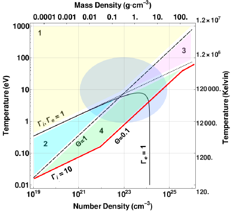
Figure 1: Parameter regimes of fully ionized hydrogen plasma. The solid black line is the boundary between weak and strong electron coupling $\Gamma_{e}=1$ and turns over due to the electron degeneracy; the dotted lined is the separation between weak and strong ion coupling $\Gamma_{i}=1$; and the dashed line is the separation between classical and degenerate electrons $\Theta=1$. The darker blue oval denotes the sector of WDM. Region 1 (yellow) is classical weakly coupled plasma; region 2 (light blue) is characterized by classical strong coupling; region 3 (pink) by quantum weak coupling, and region 4 (green) by both quantum electrons and strongly-coupled ions. We expect the theory presented here to apply to each region 1-4. The red line demarcates the region of validity of plasma-type transport theories; beyond this is the regime of condensed matter.

II A Kinetic Equation for Transport in WDM

II.1 The Uehling-Uhlenbeck Collision Operator

We consider the collision integral from the right hand side of the BUU equation (Uehling and Uhlenbeck, 1933),

$$C_{q}^{ss^{\prime}}=\int d\boldsymbol{v}^{\prime}d\Omega\frac{d\sigma}{d\Omega}u\biggl{[}\hat{f_{s}}\hat{f_{s^{\prime}}}\left(1+\theta_{s}f_{s}\right)\left(1+\theta_{s^{\prime}}f_{s^{\prime}}\right)$$

$$-f_{s}f_{s^{\prime}}\left(1+\theta_{s}\hat{f_{s}}\right)\left(1+\theta_{s}\hat{f_{s^{\prime}}}\right)\biggr{]}$$ (4)

where the “hatted” quantities $\hat{f_{s}}$ are evaluated at the post-collision velocity $\hat{\boldsymbol{v}}=\boldsymbol{v}+\Delta\boldsymbol{v}$ and $\theta_{s}=(\pm 1/g_{s})(h/m_{s})^{3}$ where $g_{s}$ is an integer accounting for particle statistics with $g_{s}=g_{e}=2$ for electrons, the $+$ sign corresponds with Bosons and the $-$ sign with Fermions. Calculation of $d\sigma/d\Omega$ is carried out via a partial wave expansion in terms of the phase shifts $\delta_{l}(\eta)$. The determination of the phase shifts from the Schrödinger equation is discussed in Appendix A.

The BUU equation describes the evolution of the Wigner quasi-probability distribution function $f_{s}$. It was originally proposed as an extension of the Boltzmann equation to account for degeneracy (Uehling and Uhlenbeck, 1933), but a consistent derivation of the equation was not accomplished for some time. Early methods involved applying the BBGKY hierarchy to the kinetic equation for the Wigner function and often fell short of fully obtaining the BUU equation, i.e. to include the $\theta_{s}$ terms (Hoffman et al., 1965; Imam-Rahajoe and Curtiss, 1967). Ultimately, a derivation was carried out using the BBGKY hierarchy in the density operator formalism (Boercker and Dufty, 1979). This required a modification of the typical weak-correlation assumption in derivations of the Boltzmann equation. Instead of neglecting three-body correlations entirely, Boercker and Dufty included the quantum correlations of two scattering particles with a third spectator particle to preserve Fermion anti-symmetry, without including correlations due to the interaction. By this method they self-consistently derived the BUU equation with the statistical $\theta_{s}$ factors, but came to the conclusion that the degeneracy must simultaneously affect the scattering cross section in addition to the statistical availability of scattering states encapsulated in the $\theta_{s}$ terms.

The BUU equation as originally formulated is applicable to moderately dense gases in which degeneracy is present but the amount of correlation is small. In the case of WDM, the equation has several deficiencies. First, it depends on the degree of degeneracy, which in turn depends on the electron number density and therefore the average ionization state of the system, which must be provided as an input. Second, in a plasma it is well known that transport rates predicted by equation (4) diverge if the cross section is computed using the Coulomb potential because the Coulomb force is of an infinite range. This is typically resolved in an ad hoc manner by enforcing a large distance limit on the impact parameter. Third, the derivation of the BUU equation, while including correlations due to Fermi statistics, does not allow for correlations due to the interaction and thus applies only in the limit of weak coupling. The remainder of this section describes how all three deficiencies can be addressed in a consistent fashion in the WDM regime.

For a tenuous and hot (read classical and weakly coupled) plasma the equilibrium ionization state is determined by the Saha equation (Saha, 1921). The divergence in the Coulomb logarithm is related to the neglect of correlation: in plasmas the collective affect of the surrounding plasma introduces Debye screening that limits the range of the interaction. A recent approach called “mean force kinetic theory” has derived a self-consistent approach to plasmas through a new expansion parameter of the BBGKY hierarchy (Baalrud and Daligault, 2019). In standard derivations of the Boltzmann equation, the BBGKY hierarchy is truncated via neglecting correlations involving three or more particles and making certain assumptions about two-particle correlations. In mean-force kinetic theory the BBGKY hierarchy is re-arranged in terms of an expansion parameter that is the difference between the exact non-equilibrium distribution function and the its equilibrium limit. The hierarchy is then truncated by assuming this difference is negligible for reduced distribution functions in three or more particle coordinates; i.e. that the high order correlations take their equilibrium values. The result is a collision integral identical in form to that of the Boltzmann equation, but in which the scattering particles interact through the potential of mean force. In addition, there is a term on the left hand side of the kinetic equation that enforces the non-ideality of the equilibrium limit in the equation of state. The result is capable of describing transport in weak to moderately coupled plasmas ($\Gamma\lesssim 20$) based on the equilibrium structural properties of the plasma.

II.2 The Quantum Potential of Mean Force

Extending mean-force kinetic theory to include quantum effects is complicated by two issues: the exclusion principle complicates the mathematics of the necessary statistical averaging, and more significantly the uncertainty principle muddles the very meaning of a potential of mean force. Classically, the mean force is the force experienced between two particles at rest with a given separation, with a statistical averaging over all of the remaining particles in the plasma at equilibrium. In the quantum case, knowing particles are “at rest with a given separation” is impossible according to the uncertainty principle. Mathematically, this prevents factoring of the kinetic and potential (configuration) terms in the equilibrium density matrix, and ultimately prevents a general derivation of the potential of mean force by extension of known classical means.

Despite this complication, the potential of mean-force must have some meaning in at least a semi-classical sense. An electron-ion pair will still induce well-defined correlations in the plasma, and these correlations can in turn influence the force felt by the interacting pair at least over the average of many scattering events at many velocities. This is reflected in the the screened potential

$$U_{{\rm sc}}(r)=\frac{\phi(r)}{k_{{\rm B}}T}{\rm e}^{-r/\lambda_{{\rm sc}}}$$ (5)

with degeneracy-dependent screening length (as per (Melrose and Mushtaq, 2010))

$$\lambda_{{\rm sc}}^{2}=\lambda_{{\rm D}}^{2}\sqrt{\frac{{\rm Li}_{3/2}\left(-\xi\right)}{{\rm Li}_{1/2}\left(-\xi\right)}}$$ (6)

which can be seen as a weak-correlation limit of the potential of mean force both for classical and quantum plasmas. The essential challenge of applying the mean force concept to WDM is how to encapsulate this effect in a binary potential when the coupling is no longer weak. It has long been known that weak correlations influence the potential in the form of plasma screening in both the classical (Debye-Huckel) and quantum (Thomas-Fermi limits). One other classical derivation of the potential of mean force is via the Ornstein-Zernike equation, which defines the direct correlation function (Hansen and McDonald, 2006). Fortunately, a quantum analog of the Ornstein-Zernike equation exists, and this equation has been used successfully to calculate the equilibrium pair correlation function in WDM (Starrett and Saumon, 2012, 2013; Starrett, 2018). Furthermore, it has been used to define a quantum potential of mean force for electron-ion interactions, and this potential has been used to predict electrical conductivities with good agreement with quantum molecular dynamics simulations (Shaffer and Starrett, 2020).

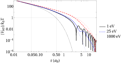
Figure 2: Electron-ion potential of mean force for solid-density ($2.7\thinspace{\rm g}\cdot{\rm cm}^{-3}$) warm dense aluminum at $1$, $25$ and $500$ eV (thick curves). In the high-temperature limit the potential approaches the screened Coulomb potential of a classical plasma (thin curves); as the temperature decreases it is altered by both degeneracy and correlations leading to different scale lengths of the potential in addition to the non-monotonic behavior.

We postulate that a quantum potential of mean force must arise naturally from the quantum mean force kinetic theory, and that this potential is that which is derived from the quantum Ornstein-Zernike equation. We turn to such a potential obtained with the quantum hypernetted-chain-approximation, coupled with an average-atom model that accounts for the structure and ionization state of the ions (Starrett and Saumon, 2012, 2013; Starrett, 2018, 2017) (subsequently referred to as the AA-TCP model for “Average-Atom Two-Component-Plasma”. This potential can be expressed as

$$V^{{\rm MF}}(r)=-\frac{Z}{r}+\int d^{3}r^{\prime}\frac{n_{e}^{{\rm ion}}(r^{\prime})}{|\boldsymbol{r}-\boldsymbol{r^{\prime}}|}$$

$$+V^{{\rm xc}}[n_{e}^{{\rm ion}}(r)]+n_{i}^{0}\int d^{3}r^{\prime}\frac{C_{ie}(|\boldsymbol{r}-\boldsymbol{r^{\prime}}|)}{-\beta}h_{ii}(r^{\prime})$$

$$+\bar{n}_{e}^{0}\int d^{3}r^{\prime}\frac{C_{ee}(|\boldsymbol{r}-\boldsymbol{r^{\prime}}|)}{-\beta}h_{ie}(r^{\prime}),$$ (7)

where $C_{ie}$ and $C_{ee}$ are the electron-ion and electron-electron direct correlation functions respectively, $h_{ie}$ and $h_{ee}$ are the electron-ion and electron-electron pair correlation functions respectively, $n_{e}^{{\rm ion}}(r)$ is the density of bound electrons, $\beta=k_{B}T$, and $V^{{\rm xc}}$ is the exchange correlation functional (in the case of (Starrett and Saumon, 2013) it is the zero-temperature Dirac exchange functional (Dirac, 1930)). Calculation of the potential requires closure, which in this case is provided by the quantum hypernetted-chain-approximation for the ion-ion correlations and through coupling to an Average-Atom model for the electron-ion correlations. Such methods can be substantially faster than full dynamical calculations such as molecular dynamics, wherein lies the primary benefit of the theory proposed in this work. In figure 2 we show example electron-ion scattering potentials from the AA-TCP model for warm dense aluminum at conditions that span the weakly coupled classical to moderately coupled degenerate regimes; see regions (1) and (4) of figure 1. The figure demonstrates the convergence of the potential of mean force with a screened Coulomb potential in the weakly-coupled limit, and the importance of correlations in the calculation of the potential in the region of moderate coupling.

III Transport Rates

Comprehensive methods to derive hydrodynamic equations, such as that of Chapman and Enskog have been developed for the Boltzmann equation (Chapman and Cowling, 1970), but their extension to the BUU equation faces considerable mathematical challenges and has not been accomplished to our knowledge. To demonstrate predictions for macroscopic transport rates, we focus on electron-ion relaxation in which the respective electron and ion distribution functions are known but the species are not in equilibrium with each other. We consider both temperature relaxation and momentum relaxation, which is related to the electrical conductivity. A restriction imposed by considering only electron-ion relaxation is that it provides only one contribution to processes such as electrical conductivity that are also influenced by electron-electron interactions. Although models such as the quantum Landau-Fokker-Planck equation have been solved using a Chapman-Enskog technique to address both contributions in a comprehensive hydrodynamic theory (Daligault, 2018), they do not address strong coupling. A recent modification has been proposed to incorporate strong coupling via a modified Coulomb logarithm computed using the potential of mean force, and finds that in the strongly degenerate regime and for high-Z systems the electron-ion collisions are dominant (Shaffer and Starrett, 2020). However, the Fokker-Planck form of the collision operator itself is only expected to apply when momentum transfer during collisions is small (i.e., weak coupling). For instance, it can be derived from a small momentum transfer expansion of the BUU equation. Here, we focus on the electron-ion relaxation using the full BUU equation in order to isolate the influence of large momentum transfer in the collision operator.

Concentrating on the electron-ion contribution also allows for a commensurable comparison with quantum MD simulations of electrical conductivity (Witte et al., 2018). Since electrons are often treated using the Born-Oppenhiemer approximation in simulations, they are also limited to treat only the electron-ion contribution to transport processes. Although electron-electron interactions are expected to contribute to the total conductivity, it is only recently becoming possible to simulate dynamic electrons in WDM following advancements in wave-packet MD (Ma et al., 2019), mixed quantum-classical MD (Simoni and Daligault, 2019; Daligault and Mozyrsky, 2018), Bohmian quantum methods (Larder et al., 2019), Kohn-Sham DFT (White and Collins, 2020) and quantum Monte Carlo (Yilmaz et al., 2020). Addressing contributions from both electron and ion dynamics will be the next step in both the theory and simulation development.

III.1 General Formalism

A binary mixture of two species $s$ and $s^{\prime}$ out of equilibrium will relax towards equilibrium through $s-s$, $s-s^{\prime}$ and $s^{\prime}-s^{\prime}$ collisions, which are modeled by moments of the collision operator (4),

$$\left\langle\chi\right\rangle^{s-s^{\prime}}=\int d\boldsymbol{v}\chi\left(\boldsymbol{v}\right)C_{qB}^{s-s^{\prime}},$$ (8)

where $\chi(\boldsymbol{v})$ is some polynomial function of the velocity. To simplify, we utilize the following properties: $d\Omega\frac{d\sigma}{d\Omega}$ is invariant under reversal of the collision, i.e. $\left(\boldsymbol{\boldsymbol{v}},\boldsymbol{v}^{\prime}\right)\leftrightarrow\left(\hat{\boldsymbol{v}},\hat{\boldsymbol{v}}^{\prime}\right)$ where $\boldsymbol{\boldsymbol{v}}\thinspace{\rm and\thinspace}\boldsymbol{v}^{\prime}$ are the pre-collision velocities of particles one and two respectively, the “hat” $\hat{}$ indicates a post-collision quantity, and the phase-space volume element is invariant, i.e. $\int d\boldsymbol{v}d\boldsymbol{v}^{\prime}=\int d\hat{\boldsymbol{v}}d\hat{\boldsymbol{v}^{\prime}}$. We thus obtain

$$\left\langle\chi\right\rangle^{s-s^{\prime}}=\int d\boldsymbol{v}\int d\Omega\frac{d\sigma}{d\Omega}u\int d\boldsymbol{v}^{\prime}\left[\chi\left(\hat{\boldsymbol{v}}\right)-\chi\left(\boldsymbol{v}\right)\right]$$

$$\times f_{s}f_{s^{\prime}}\left(1+\theta_{s}\hat{f_{s}}\right)\left(1+\theta_{s}\hat{f_{s^{\prime}}}\right).$$ (9)

Relevant $\chi\left(v\right)$ include

$$\chi\left(\boldsymbol{v}\right)=\begin{cases}1\thinspace\thinspace\thinspace\thinspace\thinspace\thinspace\thinspace\thinspace\thinspace\rightarrow&\left[\chi\left(\hat{\boldsymbol{v}}\right)-\chi\left(\boldsymbol{v}\right)\right]=0\\ m_{s}\boldsymbol{v}\thinspace\rightarrow&\left[\chi\left(\hat{\boldsymbol{v}}\right)-\chi\left(\boldsymbol{v}\right)\right]=m_{s}\boldsymbol{\Delta}v\\ m_{s}v^{2}\rightarrow&\left[\chi\left(\hat{\boldsymbol{v}}\right)-\chi\left(\boldsymbol{v}\right)\right]=m_{s}\Delta v^{2}\end{cases}$$ (10)

where $\Delta\boldsymbol{v}=\hat{\boldsymbol{v}}-\boldsymbol{v}$. Substituting variables $\boldsymbol{v}=\boldsymbol{v}^{\prime}+\boldsymbol{u}$, defining $m_{ss^{\prime}}=m_{s}m_{s^{\prime}}/(m_{s}+m_{s^{\prime}}),$ and utilizing the following relations obtained from the collision kinematics: $m_{s}\Delta\boldsymbol{v}=m_{ss^{\prime}}\Delta\boldsymbol{u},$$\Delta\boldsymbol{u}\cdot\Delta\boldsymbol{u}=-2\boldsymbol{u}\cdot\Delta\boldsymbol{u}$and $\left(2\boldsymbol{v}\cdot\Delta\boldsymbol{v}+\Delta\boldsymbol{v}^{2}\right)=(m_{ss^{\prime}}/m_{s})\Delta\boldsymbol{u}\cdot\left[\boldsymbol{v}^{\prime}+(m_{ss^{\prime}}/m_{s})\boldsymbol{u}\right],$ shows that (see (Baalrud, 2012)),

$$\chi\left(\boldsymbol{u}\right)=$$

$$\begin{cases}1\thinspace\thinspace\thinspace\thinspace\thinspace\thinspace\thinspace\thinspace\thinspace\rightarrow&\left[\chi\left(\hat{\boldsymbol{v}}\right)-\chi\left(\boldsymbol{v}\right)\right]=0\\ m_{s}\boldsymbol{v}\thinspace\rightarrow&\left[\chi\left(\hat{\boldsymbol{v}}\right)-\chi\left(\boldsymbol{v}\right)\right]=m_{ss^{\prime}}\Delta\boldsymbol{u}\\ m_{s}v^{2}\rightarrow&\left[\chi\left(\hat{\boldsymbol{v}}\right)-\chi\left(\boldsymbol{v}\right)\right]=m_{ss^{\prime}}\left(\boldsymbol{v^{\prime}}-\boldsymbol{V}_{s}+\frac{m_{ss^{\prime}}}{m_{s^{\prime}}}\boldsymbol{u}\right)\cdot\Delta\boldsymbol{u}\end{cases}$$ (11)

where

$$\Delta\boldsymbol{u}=u\left({\rm sin}\theta{\rm cos}\phi\hat{\boldsymbol{x}}+{\rm sin}\theta{\rm sin}\phi\hat{\boldsymbol{y}}-2{\rm sin}^{2}\frac{\theta}{2}\hat{\boldsymbol{u}}\right).$$ (12)

The preceding discussion and the collision operator (4) are in principle applicable to transport in any semi-classical system. As it pertains to WDM, ion-ion scattering is contained within this formalism as ion dynamics are classical and electron degeneracy effects enter only via the potential of mean force. Application of the theory to ion-ion scattering was validated in (Daligault et al., 2016). The case of the electron-electron terms requires further work due to the subtleties associated with defining the potential of mean force that are discussed in section II and will be investigated in another work. However, the model at the level to which we have developed it has immediate applicability to the case of electron-ion scattering.

III.2 The Relaxation Problem

We restrict our analysis to the class of problems in which electrons and ions in the plasma are in respective equilibrium with themselves with different fluid quantities $T_{e},\thinspace T_{i},\thinspace\boldsymbol{V}_{e}\thinspace{\rm and}\thinspace\boldsymbol{V}_{i}$, respectively. In such a system, the electron and ion fluid variables will equilibrate on a timescale long compared to the respective electron-electron and ion-ion collision times. The ions have a classical Maxwellian velocity distribution

$$f_{i}\left(\boldsymbol{v}^{\prime}\right)=\frac{n_{i}}{v_{Ti}^{3}}\frac{e^{-\left(\boldsymbol{v}^{\prime}-\boldsymbol{V}_{i}\right)^{2}/v_{Ti}^{2}}}{\pi^{3/2}}$$ (13)

and the electrons have a Fermi-Dirac velocity distribution

$$f_{e}\left(\boldsymbol{v}\right)=n_{e}\left[v_{Te}^{3}\left(-\pi^{3/2}\text{Li}_{\frac{3}{2}}(-\xi)\right)\left(1+\frac{{\rm e}^{\left(\boldsymbol{v}-\boldsymbol{V}_{e}\right)^{2}/v_{Te}^{2}}}{\xi}\right)\right]^{-1}$$ (14)

where $v_{Ts}=\sqrt{2k_{B}T_{s}/m_{s}}$ and $\xi=\exp\left(\mu/k_{B}T\right)$, the ion velocity is $\boldsymbol{v^{\prime}}$ and electron velocity is $\boldsymbol{v}$. We can write

$$f_{e}f_{i}\left(1+\theta_{e}\hat{f_{e}}\right)=\frac{n_{i}}{v_{Ti}^{3}}\frac{e^{-\left(\boldsymbol{v}^{\prime}-\boldsymbol{V}_{i}\right)^{2}/v_{Ti}^{2}}}{\pi^{3/2}}n_{e}$$

$$\times\left[v_{Te}^{3}\left(-\pi^{3/2}\text{Li}_{\frac{3}{2}}(-\xi)\right)\left(1+\frac{{\rm e}^{\left(\boldsymbol{v}^{\prime}+\boldsymbol{u}-\boldsymbol{V}_{e}\right)^{2}/v_{Te}^{2}}}{\xi}\right)\right]^{-1}$$

$$\times\left[1-\left(1+\frac{{\rm e}^{\left(\boldsymbol{v}^{\prime}+\boldsymbol{u}+(m_{ei}/m_{e})\Delta\boldsymbol{u}-\boldsymbol{V}_{e}\right)^{2}/v_{Te}^{2}}}{\xi}\right)^{-1}\right],$$ (15)

from which the relation of the factor $\left(1+\theta_{e}\hat{f_{e}}\right)$ to Pauli blocking can be seen in terms of the Fermi-Dirac occupation number: the contribution to the collision integral from collisions to or from occupied states is zero. This simplification occurs from the combination of $\theta_{e}=(-1/2)(h/m_{s})^{3}$ with the prefactor $n_{e}v_{Te}^{3}/\text{Li}_{\frac{3}{2}}(-\xi)$ in the Fermi Dirac distribution through the relation (3).

Electron-ion temperature and momentum relaxation rates depend on the energy exchange density $Q^{s-s^{\prime}}$ and friction force density $\boldsymbol{R}^{s-s^{\prime}}$, respectively. These can in turn be written in terms of the moments (9), assuming a uniform plasma, as

$$Q^{ei}=\left\langle\frac{1}{2}m_{e}\left(\boldsymbol{v}-\boldsymbol{V}_{e}\right)^{2}\right\rangle^{e-i}=\frac{3n_{e}}{2}\frac{dT_{e}}{dt}$$ (16)

(where in the last equality we have taken $\boldsymbol{V}_{e}=\boldsymbol{V}_{i}=0)$ and

$$\boldsymbol{R}^{ei}=\left\langle m_{e}\boldsymbol{v}\right\rangle^{e-i}=m_{e}\frac{d\boldsymbol{V}_{e}}{dt}$$ (17)

which, in the respective limits of $\Delta T\ll T$ and $\Delta V\ll V$ yield simple relaxation rates $dT_{e}/dt=\nu_{ei}^{(\epsilon)}\Delta T$ and $d\boldsymbol{V}_{e}/dt=\nu_{ei}^{(p)}\Delta\boldsymbol{V}$.

The integration over the ion velocity can be simplified significantly in the limit that the ion velocities are much smaller than the electron velocities: $m_{e}T_{i}\ll m_{i}T_{e}$, which (due to the small electron-to-ion mass ratio) is true when temperature differences are not extreme, coinciding with our expansion about the equilibrium state. Note that we also make the simplifying replacement $m_{ei}\approx m_{e}$. By expanding equation (15) in the limit that the electron distribution is approximately constant over the range of accessible ion velocities, the integral over the ion velocities can be carried out analytically. The evaluation of this integral differs for the calculation of $Q^{ei}$ versus $\boldsymbol{R}^{ei}$. Therefore we examine each case separately.

III.2.1 Temperature Relaxation

The energy-exchange density (16) in this case becomes

$$Q^{ei}=\int d\boldsymbol{u}\int d\Omega\frac{d\sigma}{d\Omega}u\boldsymbol{\Delta u}$$

$$\cdot\int d\boldsymbol{v}^{\prime}m_{ei}\left(\boldsymbol{v^{\prime}}+\frac{m_{ei}}{m_{i}}\boldsymbol{u}\right)f_{i}f_{e}\left(1-|\theta_{e}|\hat{f_{e}}\right).$$

Inserting equation (15), applying the expansion $|\boldsymbol{v}^{\prime}|\ll|\boldsymbol{u}|$, assuming zero drift velocities and $\left|T_{e}-T_{i}\right|\ll T_{e},T_{i}$ we perform the integral over $\boldsymbol{v}^{\prime}$ and write

$$\boldsymbol{\Delta u}\cdot\int d\boldsymbol{v}^{\prime}m_{ei}\left(\boldsymbol{v^{\prime}}+\frac{m_{ei}}{m_{i}}\boldsymbol{u}\right)f_{i}f_{e}\left(1-|\theta_{e}|\hat{f_{e}}\right)\approx$$

$$\frac{n_{e}n_{i}\eta\xi e^{-\eta^{2}}\sin^{2}\left(\frac{\theta}{2}\right)}{\pi^{3}v_{Te}\text{Li}_{\frac{3}{2}}\left(-\xi\right)\left(\xi e^{-\eta^{2}}+1\right)^{2}}$$

where $\eta\equiv u/v_{Te}$. The result is written to facilitate comparison with the classical limit,

$$Q^{ei}=-3\frac{m_{e}}{m_{i}}n_{e}\nu_{ei}^{(\epsilon)}(T_{e}-T_{i}).$$ (18)

in terms of a collision frequency

$$\nu_{ei}^{(\epsilon)}=\nu_{0}\Xi_{ei}^{(\epsilon)},$$ (19)

where

$$\nu_{0}\equiv\frac{4\sqrt{2\pi}n_{i}Z^{2}e^{4}}{3\sqrt{m_{e}}(k_{B}T_{e})^{3/2}}=2.906\times 10^{-12}\frac{Zn_{i}[{\rm m}^{-3}]}{(T_{e}[{\rm eV}])^{3/2}}$$ (20)

and a generalized Coulomb integral $\Xi_{ei}^{(\epsilon)}$. Effects of degeneracy and strong coupling are contained in the Coulomb integral,

$$\Xi_{ei}^{(\epsilon)}=\frac{1}{2}\int_{0}^{\infty}d\eta I_{\epsilon}(\eta)$$ (21)

$$I_{\epsilon}(\eta)\equiv G_{1}(\eta)\frac{\sigma_{1}^{(1)}\left(\eta,\Gamma\right)}{\sigma_{0}}$$

where

$$\sigma_{1}^{(1)}\left(\eta,\Gamma\right)=4\pi\int_{0}^{\pi}d\theta\sin^{2}\frac{\theta}{2}\sin\theta\frac{d\sigma}{d\Omega}$$ (22)

is the momentum transfer cross section, which can be written in terms of the phase shifts $\delta_{l}$ as

$$\sigma_{1}^{(1)}=\frac{4\pi}{\eta^{2}}\sum_{l=0}^{\infty}(l+1)\sin^{2}(\delta_{l+1}-\delta_{l}).$$ (23)

The function

$$G_{1}(\eta)\equiv\frac{\xi{\rm e}^{-\eta^{2}}\eta^{5}}{\left[-\text{Li}_{\frac{3}{2}}\left(-\xi\right)\right]\left(\xi e^{-\eta^{2}}+1\right)^{2}}$$ (24)

determines the relative availability of states that contribute to the scattering. This is plotted in figure 3 for several values of the degeneracy parameter $\Theta$, where it is shown that in the classical limit scattering is dominated by energy transfers around the thermal energy, and as degeneracy increases the envelope of relevant energy-transfers narrows about the Fermi energy. It should be noted that the relaxation rate obtained in equation (19) is identical to that obtained in equation (71) of reference (Daligault and Simoni, 2019) by very different means.

Figure 3: Statistical contributions to the integrands for temperature and momentum relaxation, $G_{1}$ (solid), $G_{2}$ (dashed) and $G_{3}$ (dotted), for three conditions: $\Theta=12.6$ and $\xi=0.017$ (top, weak degeneracy), $\Theta=0.85$ and $\xi=1.33$ (middle, moderate degeneracy), $\Theta=0.14$ and $\xi=1135$ (bottom, strong degeneracy). The relevant collision velocities for both momentum and temperature relaxation become narrowly centered around the Fermi velocity at strong degeneracy. The relative importance of the two different functions that contribute to momentum relaxation is degeneracy dependent.

III.2.2 Momentum Relaxation

Momentum relaxation occurs through collisions between electron and ion populations with different average velocities. The force density (17) associated with these collisions is

$$\boldsymbol{R}^{ei}=\int d\boldsymbol{u}\int d\Omega\frac{d\sigma}{d\Omega}u\int d\boldsymbol{v}^{\prime}m_{ei}\boldsymbol{\Delta u}f_{e}f_{i}\left(1+\theta_{e}\hat{f_{e}}\right).$$ (25)

Inserting equation (15), applying the expansion $|\boldsymbol{v}^{\prime}|\ll|\boldsymbol{u}|,$ and assuming $\left|T_{e}-T_{i}\right|\ll T_{e},T_{i}$, $V_{i}\ll v_{Ti}$ and $V_{e}\ll v_{Te}$, the integral over $\boldsymbol{v}^{\prime}$ can be performed analytically,

$$\int d\boldsymbol{v}^{\prime}m_{ei}f_{e}f_{i}\left(1+\theta_{e}\hat{f_{e}}\right)$$

$$\approx\frac{2m_{e}n_{e}\xi n_{i}e^{-\eta^{2}}\left[\boldsymbol{u}\cdot\boldsymbol{\Delta V}-\xi e^{-\eta^{2}}\left(\boldsymbol{\Delta u}+\boldsymbol{u}\right)\cdot\boldsymbol{\Delta V}\right]}{\pi^{3/2}v_{Te}^{5}\left[-\text{Li}_{\frac{3}{2}}\left(-\xi\right)\right]\left(\xi e^{-\eta^{2}}+1\right){}^{3}}.$$

We follow the classical example and write

$$\boldsymbol{R}^{ei}=-n_{e}m_{e}\nu_{ei}^{(p)}(\boldsymbol{V}_{e}-\boldsymbol{V}_{i})$$ (26)

where the frequency

$$\nu_{ei}^{(p)}=\nu_{0}\Xi_{ei}^{(p)}$$ (27)

involves a Coulomb integral

$$\Xi_{ei}^{(p)}=\frac{1}{2}\int_{0}^{\infty}d\eta I_{p}(\eta,\Gamma,\xi)$$

$$I_{p}(\eta,\Gamma,\xi)\equiv G_{2}(\eta,\xi)\frac{\sigma_{1}^{(1)}\left(\eta,\Gamma\right)}{\sigma_{0}}-G_{3}(\eta,\xi)\frac{\sigma_{2}^{(1)}\left(\eta,\Gamma\right)}{\sigma_{0}}$$ (28)

$$=G_{2}(\eta,\xi)\frac{\sigma_{p}(\eta,\Gamma,\xi)}{\sigma_{0}}$$ (29)

which is different from that involved in the energy-exchange density. Here, $\sigma_{1}^{(1)}$ is defined in equation (23),

$$\sigma_{2}^{(1)}\left(\eta,\Gamma\right)=4\pi\int_{0}^{\pi}d\theta\sin^{2}\frac{\theta}{2}\sin\theta\frac{d\sigma}{d\Omega}\cos\theta,$$ (30)

and

$$\sigma_{p}(\eta,\Gamma,\xi)=\sigma_{1}^{(1)}\left(\eta,\Gamma\right)-\xi{\rm e}^{-\eta^{2}}\sigma_{2}^{(1)}\left(\eta,\Gamma\right).$$ (31)

It is interesting to note that the cross section arising in the energy relaxation rate from equation (23) differs from that associated with momentum relaxation from equation (31). This is a purely quantum mechanical effect, as the cross section definitions are the same in the classical limit (Baalrud, 2012). It is also an effect that is predicted by the full BUU equation, but not the Landau-Fokker-Plank limit associated with small momentum transfer interactions (Shaffer and Starrett, 2020). The weighting functions

$$G_{2}(\eta,\xi)=\frac{\xi{\rm e}^{-\eta^{2}}\eta^{5}}{\left[-\text{Li}_{\frac{3}{2}}\left(-\xi\right)\right]\left(\xi e^{-\eta^{2}}+1\right)^{3}},$$ (32)

$$G_{3}(\eta,\xi)=\frac{\xi^{2}{\rm e}^{-2\eta^{2}}\eta^{5}}{\left[-\text{Li}_{\frac{3}{2}}\left(-\xi\right)\right]\left(\xi e^{-\eta^{2}}+1\right)^{3}},$$ (33)

are shown in figure 3 and compared with the statistical weighting factors in the case of temperature relaxation. The presence of the differing angular integrals between the energy and momentum relaxation cases warrants further discussion.

Through the use of the Wigner-3j function, $\sigma_{2}^{(1)}$ can be expanded in the phase shifts (see appendix B) as

$$\sigma_{2}^{(1)}=\frac{4\pi}{\eta^{2}}\sum_{l=0}^{\infty}\frac{\sin\delta_{l}}{4l(l+1)-3}$$

$$\times\left\{(l+1)(2l-1)\left[(l+2)\sin(\delta_{l}-2\delta_{l+2})-(2l+3)\sin(\text{$\delta_{l}$}-2\text{$\delta_{l+1}$})\right]-l^{2}(2l+3)\sin\delta_{l}\right\}.$$ (34)

While it is tempting to interpret the quantity $\sigma_{2}^{(1)}$ as a cross-section, $\sigma_{2}^{(1)}$ can become negative and therefore has no such interpretation. We will show in the next section that it is only in the combination defined in equation (31) that this interpretation is justified. We thus refer to $\sigma_{p}$ as an effective transport cross section. We note that this second term arises due to degeneracy, and has no analog in the classical relaxation problem.

III.2.3 Electrical Conductivity

The electrical conductivity is an important transport coefficient that depends largely on the electron-ion collisional momentum relaxation rate. Considering a Fermi-Dirac electron population flowing through a stationary Maxwellian ion population due to an applied electric field, the frictional force balances the electric force

$$\boldsymbol{R}_{ei}=-en_{e}\boldsymbol{E},$$ (35)

which in the form of equation (26) is connected to the current through Ohm’s law

$$\boldsymbol{J}=\sigma\boldsymbol{E}$$ (36)

where $\boldsymbol{J}=-en_{e}\boldsymbol{V}_{e}$. Using the electron-ion collisional friction [equation (26)], the resulting electrical conductivity is

$$\sigma=\frac{e^{2}n_{e}}{m_{e}\nu_{ei}^{(p)}},$$ (37)

where $\nu_{ei}^{(p)}$ is defined in equation (27). The assumption of a Fermi-Dirac electron distribution means that electron-electron (e-e) collisions do not contribute to the relaxation; distortions in the electron distribution away from equilibrium amount to a higher order approximation that could be explored e.g. through the Chapman-Enskog expansion. The e-e collisions do not contribute substantially in the degenerate regimes due to Pauli blocking, and at high temperatures the e-e contribution is well understood via the Landau-Spitzer theory. The intermediate regime where both degeneracy and e-e collisions are important is discussed by Shaffer and Starrett (Shaffer and Starrett, 2020) in the context of the quantum Fokker-Planck equation. The application of the BUU equation to this regime to relax the assumption of small-momentum-transfer collisions will require a Chapman-Enskog expansion of the BUU equation and will be addressed in further studies.

IV Results and Discussion

To illustrate the application of the model, we now turn to evaluating it, with input potentials provided by the AA-TCP model ((Starrett and Saumon, 2012, 2013)) for aluminum at a density of $2.7\thinspace{\rm g\cdot cm}^{-3}$, over a range of temperatures spanning from the degenerate moderately coupled to classical weakly-coupled regimes. However, firstly we demonstrate the behaviors of the two functions $\sigma_{2}^{(1)}$ and $\sigma_{1}^{(1)}$ in figure 4 at two example temperature-density points. The combined influence of the negative values of $\sigma_{2}^{(1)}$ and the preceding negative sign in equation (28) leads to interesting behavior in the integrand for the Coulomb integral. The full integrand of equation (28) is shown in figure 5 where it is seen that the resulting integrals are positive, as required. Note that the integrands are peaked functions; broad and peaked near the thermal velocity $v_{Ts}$ in the classical limit, and narrow with peak near the Fermi velocity in the degenerate limit. Also note that $I_{p}$ and $I_{\epsilon}$ are identical in the classical limit, but differ substantially in the degenerate case due to the presence of the $\sigma_{2}^{(1)}$ factor.

Figure 4: Functions $\sigma_{1}^{(1)}$ and $\sigma_{2}^{(1)}$ calculated using the PMF for solid density $(2.7\thinspace{\rm g}\cdot{\rm cm}^{-3})$ aluminum at $1000\thinspace{\rm eV}$ (top) and $1\thinspace{\rm eV}$ (bottom). While $\sigma_{2}^{(1)}$ plays the role of a cross section, it is evident from its negative value at many velocities that it is not one. Interestingly, it behaves (only approximately) inversely to the momentum transfer cross section $\sigma_{1}^{(1)}$. While $\sigma_{2}^{(1)}$ is non-zero at high temperatures, its influence is negligible due to the suppression of the term that contains it when $T\gg E_{{\rm F}}$.

Figure 5: Integrands ($I_{\epsilon}(\eta)$ solid and $I_{p}(\eta)$ dashed) appearing in equations (21) and (28) for aluminum at $2.7\thinspace{\rm g\cdot cm}^{-3}$ at three different temperatures: $100\thinspace{\rm eV}$ ($\Theta\gg 1$) (top), $10\thinspace{\rm eV}$ ($\Theta\sim 1$) (middle), $1\thinspace{\rm eV}$ ($\Theta\ll 1$) (bottom).

IV.1 Relaxation Rates in Solid Density Aluminum Plasma

Figure 6 shows a comparison of the momentum and energy relaxation rates. Each model is compared with the well-established Landau-Spitzer result (Spitzer, 1956), which in the limit $m_{e}T_{i}\ll m_{i}T_{e}$ reduces to

$$\nu_{ei}^{{\rm LS}}\approx\nu_{0}\ln\Lambda_{{\rm LS}}$$ (38)

which has been verified in the classical limit given sufficiently weak coupling (Trintchouk et al., 2003; Kuritsyn et al., 2006). The relaxation rate predicted by the LFP model is(see equations 14-17 of (Daligault, 2016)),

$$\nu_{ei}^{{\rm LFP}}=\nu_{0}\left(\ln\Lambda_{{\rm LFP}}\frac{\xi}{1+\xi}\frac{3\sqrt{\pi}\Theta^{3/2}}{4}\right).$$ (39)

We further note that our expression for the temperature relaxation rate (given by equations (18)-(23)) is the same as that recently obtained by a substantially different by Daligault and Simoni (see equations (71)-(75) of (Daligault and Simoni, 2019)) if the potential of mean force is used for calculating the transport cross section there. This equivalency can be seen through use of the relation $n_{e}\left(h/\sqrt{\pi}m_{e}v_{Te}\right)^{3}=-2{\rm Li}_{3/2}\left(-\xi\right)$ from the normalization of the Fermi-Dirac distribution.

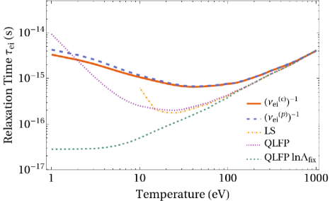
Figure 6: Electron-ion collisional relaxation times ($\tau=\nu_{ei,}^{-1}$) as a function of temperature in solid density ($2.7\thinspace{\rm g\cdot cm}^{-3}$) aluminum.

At a given density, as temperature decreases the Coulomb logarithm will eventually reach zero due to neglect of strong coupling physics. The resulting divergence of the Landau-Spitzer result due to the presence of the (inverse) Coulomb logarithm

$$\ln\Lambda_{{\rm LS}}=\ln\frac{b_{{\rm max}}}{b_{{\rm min}}}.$$ (40)

The maximum impact parameter is modeled as the larger of the screening length $\lambda_{{\rm sc}}$[equation (6)] or the Wigner-Seitz radius $a=(3/4\pi n_{i})^{1/3}$, and the minimum is the larger of the classical distance of closest approach $r_{L}=e^{2}/k_{B}T$ or the thermal de Broglie wavelength $\lambda_{{\rm dB}}=\hbar/\left(m_{e}k_{{\rm B}}T_{e}\right)^{1/2}$ (Lee and More, 1984). In WDM, the vanishing Coulomb logarithm is often resolved through the modification (see e.g. (Lee and More, 1984))

$$\ln\Lambda_{{\rm LFP}}=\frac{1}{2}\ln\left(1+\frac{b_{{\rm max}}^{2}}{b_{{\rm min}}^{2}}\right),$$ (41)

which we apply in our evaluation of the LFP model. This is often further altered, as is done in the Lee-Moore conductivity model (Lee and More, 1984), by enforcing that the minimum value of the Coulomb logarithm be 2:

$$\ln\Lambda_{{\rm fix}}={\rm max}\left[2,\frac{1}{2}\ln\left(1+\frac{b_{{\rm max}}^{2}}{b_{{\rm min}}^{2}}\right)\right].$$ (42)

The approximations inherent in this approach are two-fold: small-angle collisions must be assumed to obtain the LFP equation, and the choice of maximum and minimum impact parameters represents an uncontrolled expansion in the strongly coupled regime. The convergent kinetic equation in our approach avoids these limitations.

Figure 6 confirms the expectation that all expressions agree at high temperatures associated with the the weakly-coupled classical regime, while at low temperature the models differ as a result of the different levels of inclusion of the physics of strong coupling and degeneracy. In each case there is a minimum in the relaxation time. In all cases except the Landau-Spitzer result, this minimum can be attributed to a combination of both degeneracy and strong coupling: strong coupling increases the collisionality of the system while the onset of degeneracy reduces the collisionality through Pauli blocking. The decreased level of ionization at lower temperatures also reduces the collisionality. If the density is less than $10^{23}\thinspace{\rm cm}^{-3}$ as temperature is reduced the plasma will first become strongly coupled and then degenerate, and if the density is greater than $10^{23}\thinspace{\rm cm}^{-3}$ the electrons will be degenerate when the transition to strong coupling occurs.

The quantum mean force model predicts that the relaxation time $\tau$ for energy and momentum relaxation do not have the same behavior with temperature. The rates are equal in the classical limit as expected, but differ for lower temperatures when degeneracy arises. Generally, the rates are smaller for energy relaxation, with the maximum difference being a factor of $\sim 2$. Experimental validation of this phenomenon will require accurate measurements of both momentum and temperature relaxation rates in WDM, a matter of considerable difficulty. However, further consideration of the physical basis for the difference between momentum and temperature relaxation is called for, and perhaps computational methods will prove to be effective to this end. This effect is not present in the LS or QLFP theories and is a result of allowing for strong quantum collisions, which these theories do not account for. The LS theory ignores both degeneracy and large-angle scattering. The QLFP theory extends further into the degenerate regime and has fixed the vanishing Coulomb log, but does not account for either correlations or large-angle scattering when there is strong Coulomb coupling. The divergence between the QLFP results using the two different prescriptions for the Coulomb log illustrates the lack of strong-coupling physics in the method.

IV.2 Electrical Conductivity of Solid-Density Aluminum Plasma

We proceed to evaluate the electrical conductivity according to equation (37) for aluminum at $2.7\thinspace{\rm g\cdot cm}^{-3}$, as a demonstration of the model in a regime marked by partial ionization and a simultaneous transition from weak to strong coupling and classical to degenerate statistics. For comparison we select the Lee-Moore model, the model of Shaffer and Starrett (Shaffer and Starrett, 2020) and the QMD simulations of Witte et al (Witte et al., 2018). The electrical conductivity coefficient predicted by the LM model (Lee and More, 1984) is

$$\sigma_{e}=\frac{ne^{2}}{m}\left\{\frac{3\sqrt{m}(kT)^{3/2}}{2\sqrt{2}\pi Z^{2}n_{i}e^{4}\ln\Lambda_{{\rm fix}}}\right\}\frac{4}{3}\frac{\int_{0}^{\infty}\frac{t^{2}dt}{1+\exp(t-\mu/kT)}}{\int_{0}^{\infty}\frac{t^{1/2}dt}{1+\exp(t-\mu/kT)}}$$ (43)

which we relate to the friction force density $\boldsymbol{R}$ and thus the scattering rate: $\nu_{ei}^{(p)}=e^{2}n_{e}/\sigma m_{e}$ giving

$$\nu_{ei}^{{\rm LM}}=\nu_{0}\left[\ln\Lambda_{{\rm fix}}\frac{{\rm Li}_{3/2}(-\xi)}{{\rm Li}_{3}(-\xi)}\right].$$ (44)

The Starrett and Shaffer model similarly uses the quantum potential of mean force to mediate scattering, but in the context of the QLFP equation. In order to introduce the effect of large-angle collisions into the model they introduce a Coulomb logarithm defined via the relaxation-time approximation (RTA) which we will refer to as ${\rm ln}\Lambda_{{\rm SS}}$. For a commensurate comparison with our method (where we assume a Fermi distribution for the electrons) and the QMD simulations, we neglect the higher order Chapman-Enskog corrections associated with electron-electron interactions that can be obtained in the SS model. The electron-ion contribution corresponds with the first order of the Chapman-Enskog expansion,

$$\sigma_{{\rm 1,qLFP}}=\frac{3(4\pi\epsilon_{0})^{2}(k_{B}T)^{3/2}}{4\sqrt{2\pi m_{e}}Ze^{2}\ln\Lambda_{{\rm ss}}}\frac{{\rm Li_{3/2}(-\xi)}}{{\rm Li}_{0}(-\xi)}$$

With the identification of

$${\rm Li}_{0}(-\xi)=\frac{-\xi}{1+\xi}$$

and (from 39)

$$\ln\Lambda\frac{\xi}{1+\xi}\frac{3\sqrt{\pi}\Theta^{3/2}}{4}\rightarrow\ln\Lambda,$$

and equation (3) it can be seen this is equivalent in form to equation (37) with the difference being the Coulomb logarithm.

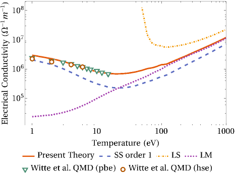
Figure 7: Electron-ion contribution to the electrical conductivity of solid density aluminum ($2.7\thinspace{\rm g\cdot cm}^{-3}$) as derived through the current work (solid line) the Starrett and Shaffer model evaluated at first order in the Chapman-Enskog expansion (dashed line), the Lee-More model (dotted line), and the LS conductivity (dot-dashed line), along with QMD results of Witte et al (Witte et al., 2018) using the Perdew–Burke-Ernzerhof and Heyd–Scuseria–Ernzerhof exchange-correlation functionals.

The resulting predictions for the conductivity are shown in figure 7. Similarly to the relaxation times, there is a minimum in the conductivity near the Fermi temperature. This again can be attributed to both correlations and Pauli blocking (Shaffer and Starrett, 2020). Also as in the case of the relaxation times, the LS theory fails to accurately predict the conductivity when degeneracy and correlations are important, as expected. Furthermore, the commonly used Lee-Moore theory performs poorly as a result of the correlations. Interestingly, the Lee-Moore theory can be reproduced by replacing the Coulomb logarithm in the standard QLFP formulation with the fixed version prescribed in the Lee-Moore theory. Although we focus on the electron-ion contribution, it is known that electron-electron interactions cause a contribution of comparable magnitude in the classical weakly coupled limit (the Spitzer correction) (Spitzer, 1956). However, it can be expected that e-e collisions will be greatly suppressed below the Fermi temperature due to Pauli blocking and therefore the corrections due to a higher-order Chapman Enskog expansion will be diminished at lower temperatures. Indeed, this is seen for the QLFP equation (Daligault, 2018).

More interesting are the comparisons of the present theory with the Shaffer-Starrett formulation of the QLFP theory (Shaffer and Starrett, 2020), and with the QMD simulations of Witte et al. (Witte et al., 2018). The QLFP equation being the limit of the BUU equation with only small-angle scattering, it may be expected that these formulations should agree in the limit of weak coupling. However, the present theory and the SS theory differ in their treatment of the potential of mean force, and the curves appear to not yet have reached this limiting behavior at $1000\thinspace{\rm eV}$. The QMD simulations also make an interesting direct comparison. QMD simulations do not directly include e-e collisions because they use the Born-Oppenhiemer approximation, but account for some level of the electronic interactions through the mean field. (Desjarlais et al., 2017). Thus, it seems most appropriate to compare the QMD simulations with theories evaluated to treat only the electron-ion interactions, as is done in figure 7. Indeed, the agreement with these simulations is remarkable for most of the range of available data, from $15\thinspace{\rm eV}$ down to approximately $2\thinspace{\rm eV}$. At the lowest temperatures the predictions begin to diverge, but it is unclear at these very low temperatures whether the BUU equation can be expected to be valid as higher-order quantum correlations come into play. To fully address the contribution of e-e collisions will require solutions of the BUU equation at higher orders of the Chapman-Enskog expansion.

The good agreement between QMD and the BUU predictions provides evidence that large momentum transfer collisions, and the associated second (quantum) contribution to the momentum scattering rate [equation (30)] are real and significant effects influencing the electrical conductivity. This points to important physics beyond what is captured by the QLFP theory, or its modifications, as is shown by comparing with the first-order Chapman-Enskog solution of the Shaffer-Starrett model from (Shaffer and Starrett, 2020) (the first order of this method is equivalent to the electron-ion relaxation model described in the previous section, and therefore provides a commensurate comparison). At the same time, it is also important to note that electron-electron contributions may influence the total conductivity at these conditions. Shaffer and Starrett predict these to make order-unity contributions over the range of conditions plotted in figure 7 (Shaffer and Starrett, 2020). Further development will be required to evaluate this contribution from the BUU equation, as well as to provide a conclusive test using QMD.

V Conclusions

We have presented a model for transport in plasmas with weak to moderate Coulomb coupling and weak to moderate electron degeneracy. The model is based on the quantum Boltzmann equation of Uehling and Uhlenbeck, in which the two-body scattering is mediated by the equilibrium potential of mean force. This incorporates correlations in the equilibrium limit while maintaining the simplicity of binary collisions in the dynamical equation. This is relevant to electron-ion collisions in WDM. As input into the model, we utilized an existing model for the potential of mean force derived from the quantum Ornstein-Zernike equations and an average-atom quantum hypernetted-chain-approximation model (Starrett and Saumon, 2012, 2013; Starrett, 2018).

The model was used to compute momentum and energy relaxation rates. The transport coefficients were written analogously to the classical Landau-Spitzer (LS) result in terms of a “Coulomb integral” that takes the place of the traditional Coulomb logarithm. The Coulomb integral depends on the level of degeneracy, and Coulomb coupling enters through the calculation of the momentum-transfer cross section solving the Schrödinger equation with the PMF as the scattering potential. The momentum relaxation rate was found to differ from temperature relaxation in that it depends on a different transport cross section, which includes a term that is solely associated with degeneracy, and has no analog in the classical limit. The dependence of the integrands of the Coulomb integrals on the level of degeneracy was compared for the temperature and momentum relaxation cases.

We concluded by calculating the temperature and momentum relaxation rates and electrical conductivity in solid density aluminum plasma over a range of temperatures that covered the transitions between weak and moderate coupling and weak and moderate degeneracy. Predictions were compared with other leading models. It was found that all models behave as expected in the classical weak-coupling limit, and diverge widely in the limit of a degenerate moderately-coupled plasma. We assessed the relative importance of the different relevant physical processes that complicate the problem as degeneracy and coupling simultaneously increase: diffraction, Pauli blocking, correlations, and large-angle scattering. Interestingly, in the degenerate regime there is a quantitative difference in the predicted relaxation rates for momentum versus energy. Ultimately, current and near-future experimental measurements (Cho et al., 2016; Glenzer et al., 2016; Zaghoo et al., 2019) and ab-initio simulations (Daligault and Mozyrsky, 2018; Larder et al., 2019; Ma et al., 2019; Simoni and Daligault, 2019; White and Collins, 2020; Yilmaz et al., 2020) will be able to shed light on the applicability of the different models of transport for WDM.

This work can be improved through inclusion of electron-electron collisions and higher-order terms of a Chapman-Enskog expansion. Additionally, further work will be required to obtain a rigorously derived convergent kinetic equation with the appropriate potential of mean force. Finally, recent and upcoming experimental measurements of electrical conductivity and temperature relaxation (Cho et al., 2016; Zaghoo et al., 2019) may soon open the door for discrimination between the validity of the various models of relaxation in WDM. This will enhance our understanding of the basic physics of WDM, and allow increased fidelity in the rapid calculation of transport coefficients for use in hydrodynamic simulations of naturally and experimentally occurring WDM.

Appendix A Determination of Phase Shifts

Solution of the scattering problem comes down to solution of the radial Schrödinger equation (Landau and Lifshitz, 1965)

$$\frac{d^{2}u_{l}}{dr^{2}}+\left[k^{2}-\frac{l\left(l+1\right)}{r^{2}}-\frac{2m_{ei}}{\hbar^{2}}W^{(2)}\left(r\right)\right]u_{l}=0,$$

For each angular quantum number $l$ there is a phase shift $\delta_{l}$ that can be extracted from the asymptotic behavior of the wavefunction $u_{l}$ beyond the range of the potential at point $R$ (defined as a point beyond with the influence of the potential on the wavefunction is negligible) through the relation:

$$\tan\delta_{l}=\frac{kRj_{l}^{\prime}\left(kR\right)-\beta_{l}j_{l}\left(kR\right)}{kRy_{l}^{\prime}\left(kR\right)-\beta_{l}y_{l}\left(kR\right)}$$

with

$$\beta_{l}=\frac{1}{u_{l}/r}\left.\frac{d\left(u_{l}/r\right)}{dr}\right|_{r=R}$$

where $j_{l}$ ($y_{l}$) are the spherical Bessel (Neumann) functions. For $l>30$ it is faster and still accurate to use the WKB phase shifts

$$\delta_{l}^{({\rm WKB)}}=-\int_{(l+1/2)/k}^{\infty}\sqrt{k^{2}-\frac{(l+1/2)^{2}}{r^{2}}dr}$$

$$+\int_{r_{C}}^{\infty}\sqrt{k^{2}-\frac{(l+1/2)^{2}}{r^{2}}-\frac{2m_{e}}{\hbar^{2}}U(r)}dr$$ (45)

Appendix B Simplification of Cross Sections

Cross sections are calculated in the partial wave expansion

$$\frac{d\sigma}{d\Omega}=\left|\frac{1}{2ik}\sum_{l=0}^{\infty}\left(2l+1\right)\left({\rm e}^{2i\delta_{l}}-1\right)P_{l}\left({\rm cos}\theta\right)\right|^{2},$$ (46)

where the phase shifts $\delta_{l}$ are calculated from solution of the Schrödinger equation for the given potential. This can be written as a double sum

$$\frac{d\sigma}{d\Omega}=\frac{1}{k^{2}}\sum_{n=0}^{\infty}\sum_{m=0}^{\infty}\left(2m+1\right)\left(2n+1\right)$$

$$\times{\rm e}^{i\left(\delta_{m}-\delta_{n}\right)}\sin\delta_{m}\sin\delta_{n}{\rm P}_{m}(\cos\theta){\rm P}_{n}(\cos\theta)$$

which inserted into equation (30) results in

$$\sigma_{2}^{(1)}\left(\eta,\Gamma\right)=\frac{4\pi}{k^{2}}$$

$$\times\sum_{n=0}^{\infty}\sum_{m=0}^{\infty}\left(2m+1\right)\left(2n+1\right){\rm e}^{i\left(\delta_{m}-\delta_{n}\right)}\sin\delta_{m}\sin\delta_{n}$$

$$\times\int_{0}^{\pi}d\theta\sin^{2}\frac{\theta}{2}\sin\theta\cos\theta{\rm P}_{m}(\cos\theta){\rm P}_{n}(\cos\theta).$$

Taking advantage of the properties of the Legendre polynomials this is

$$\frac{4\pi}{k^{2}}\sum_{n=0}^{\infty}\sum_{m=0}^{\infty}\left(2m+1\right)\left(2n+1\right){\rm e}^{i\left(\delta_{m}-\delta_{n}\right)}\sin\delta_{m}\sin\delta_{n}$$

$$\times\frac{1}{2}\int_{0}^{\pi}\sin\theta\left[P_{1}(\cos\theta)-\frac{2}{3}P_{2}(\cos\theta)-\frac{P_{0}}{3}\right]$$

$$\times P_{m}(\cos\theta)P_{n}(\cos\theta)d\theta,$$

Finally, with the identity

$$\int_{0}^{\pi}d\theta\sin\theta P_{l}(\cos\theta)P_{m}(\cos\theta)P_{n}(\cos\theta)=2\left(\begin{array}[]{ccc}l&m&n\\ 0&0&0\end{array}\right)^{2},$$ (47)

where $\left(\begin{array}[]{c}\cdots\\ \cdots\end{array}\right)$ is the Wigner 3j symbol and using the specific values for $l=0,\thinspace 1,\thinspace{\rm and}\thinspace 2$, we obtain equation (34).

References

- Glenzer et al. (2016) S. H. Glenzer, L. B. Fletcher, E. Galtier, B. Nagler, R. Alonso-Mori, B. Barbrel, S. B. Brown, D. A. Chapman, Z. Chen, C. B. Curry, F. Fiuza, E. Gamboa, M. Gauthier, D. O. Gericke, A. Gleason, S. Goede, E. Granados, P. Heimann, J. Kim, D. Kraus, M. J. MacDonald, A. J. Mackinnon, R. Mishra, A. Ravasio, C. Roedel, P. Sperling, W. Schumaker, Y. Y. Tsui, J. Vorberger, U. Zastrau, A. Fry, W. E. White, J. B. Hasting, and H. J. Lee, Journal of Physics B Atomic Molecular Physics 49, 092001 (2016).
- Riley (2018) D. Riley, Plasma Physics and Controlled Fusion 60, 014033 (2018).
- Mančić (2010) A. Mančić, in Journal of Physics Conference Series, Vol. 257 (2010) p. 012009.
- Redmer et al. (2008) R. Redmer, N. Nettelmann, B. Holst, A. Kietzmann, and M. French, “Quantum Molecular Dynamics Simulations for Warm Dense Matter and Applications in Astrophysics,” in Condensed Matter Physics in the Prime of 21st Century: Phenomena, Materials, Ideas, Methods - 43rd Karpacz Winter School of Theoretical Physics (World Scientific Publishing Co. Pte. Ltd., 2008) pp. 223–236.
- Koenig et al. (2005) M. Koenig, A. Benuzzi-Mounaix, A. Ravasio, T. Vinci, N. Ozaki, S. Lepape, D. Batani, G. Huser, T. Hall, D. Hicks, A. MacKinnon, P. Patel, H. S. Park, T. Boehly, M. Borghesi, S. Kar, and L. Romagnani, Plasma Physics and Controlled Fusion 47, B441 (2005).
- Hu et al. (2015) S. X. Hu, V. N. Goncharov, T. R. Boehly, R. L. McCrory, S. Skupsky, L. A. Collins, J. D. Kress, and B. Militzer, Physics of Plasmas 22, 056304 (2015).
- Uehling and Uhlenbeck (1933) E. A. Uehling and G. E. Uhlenbeck, Physical Review 43, 552 (1933).
- Baalrud and Daligault (2019) S. D. Baalrud and J. Daligault, Physics of Plasmas 26, 082106 (2019), https://doi.org/10.1063/1.5095655 .
- Melrose and Mushtaq (2010) D. B. Melrose and A. Mushtaq, Phys. Rev. E 82, 056402 (2010).
- Spitzer (1956) L. Spitzer, Physics of Fully Ionized Gases (Interscience Publishers, Inc., New York, 1956).
- Daligault (2016) J. Daligault, Physics of Plasmas 23, 032706 (2016).
- Baalrud and Daligault (2013) S. D. Baalrud and J. Daligault, Physical Review Letters 110, 235001 (2013), arXiv:1303.3202 [physics.plasm-ph] .
- Baalrud and Daligault (2014) S. D. Baalrud and J. Daligault, Physics of Plasmas 21, 055707 (2014), arXiv:1403.1882 [physics.plasm-ph] .
- Daligault et al. (2016) J. Daligault, S. D. Baalrud, C. E. Starrett, D. Saumon, and T. Sjostrom, Physical Review Letters 116, 075002 (2016).
- Daligault (2018) J. Daligault, Physics of Plasmas 25, 082703 (2018), https://doi.org/10.1063/1.5045330 .
- Gericke et al. (2002) D. O. Gericke, M. S. Murillo, and M. Schlanges, Phys. Rev. E 65, 036418 (2002).
- Lee and More (1984) Y. T. Lee and R. M. More, Physics of Fluids 27, 1273 (1984).
- Starrett (2018) C. E. Starrett, Physics of Plasmas 25, 092707 (2018), arXiv:1808.07153 [physics.plasm-ph] .
- Daligault and Dimonte (2009) J. Daligault and G. Dimonte, Phys. Rev. E 79, 056403 (2009), arXiv:0902.1997 [physics.plasm-ph] .
- Lampe (1968) M. Lampe, Phys. Rev. 170, 306 (1968).
- Scullard et al. (2018) C. R. Scullard, S. Serna, L. X. Benedict, C. L. Ellison, and F. R. Graziani, Phys. Rev. E 97, 013205 (2018), arXiv:1710.00972 [physics.plasm-ph] .
- Brown et al. (2005) L. S. Brown, D. L. Preston, and R. L. Singleton, Jr., Physics Reports 410, 237 (2005), arXiv:physics/0501084 [physics.plasm-ph] .
- Brown and Singleton (2007) L. S. Brown and R. L. Singleton, Jr., Phys. Rev. E 76, 066404 (2007), arXiv:0707.2370 [physics.plasm-ph] .
- Balzer and Bonitz (2013) K. Balzer and M. Bonitz, Nonequilibrium Green’s Functions Approach to Inhomogeneous Systems, LNP, Vol. 867 (Springer, Berlin, Heidelberg, 2013).
- Bonitz (2016) M. Bonitz, Quantum Kinetic Theory (Springer, Cham, Switzerland, 2016).
- Starrett and Saumon (2013) C. E. Starrett and D. Saumon, Phys. Rev. E 87, 013104 (2013).
- Daligault and Simoni (2019) J. Daligault and J. Simoni, Phys. Rev. E 100, 043201 (2019).
- Witte et al. (2018) B. B. L. Witte, P. Sperling, M. French, V. Recoules, S. H. Glenzer, and R. Redmer, Physics of Plasmas 25, 056901 (2018).
- Hoffman et al. (1965) D. K. Hoffman, J. J. Mueller, and C. F. Curtiss, Journal of Chemical Physics 43, 2878 (1965).
- Imam-Rahajoe and Curtiss (1967) S. Imam-Rahajoe and C. F. Curtiss, Journal of Chemical Physics 47, 5269 (1967).
- Boercker and Dufty (1979) D. B. Boercker and J. W. Dufty, Annals of Physics 119, 43 (1979).
- Saha (1921) M. N. Saha, Proceedings of the Royal Society A: Mathematical, Physical and Engineering Sciences 99, 135 (1921).
- Hansen and McDonald (2006) J. Hansen and I. McDonald, Theory of Simple Liquids, 3rd ed. (Academic Press, Oxford, 2006).
- Starrett and Saumon (2012) C. E. Starrett and D. Saumon, Phys. Rev. E 85, 026403 (2012).
- Shaffer and Starrett (2020) N. R. Shaffer and C. E. Starrett, Phys. Rev. E 101, 053204 (2020).
- Starrett (2017) C. E. Starrett, High Energy Density Physics 25, 8 (2017), arXiv:1708.06647 [physics.plasm-ph] .
- Dirac (1930) P. A. M. Dirac, Proceedings of the Cambridge Philosophical Society 26, 376 (1930).
- Chapman and Cowling (1970) S. Chapman and T. G. Cowling, The Mathematical Theory of Non-Uniform Gases, 3rd ed. (Cambridge University Press, 1970).
- Ma et al. (2019) Q. Ma, J. Dai, D. Kang, M. S. Murillo, Y. Hou, Z. Zhao, and J. Yuan, Phys. Rev. Lett. 122, 015001 (2019).
- Simoni and Daligault (2019) J. Simoni and J. Daligault, Phys. Rev. Lett. 122, 205001 (2019), arXiv:1904.04450 [physics.plasm-ph] .
- Daligault and Mozyrsky (2018) J. Daligault and D. Mozyrsky, Phys. Rev. B 98, 205120 (2018), arXiv:1708.06679 [physics.comp-ph] .
- Larder et al. (2019) B. Larder, D. O. Gericke, S. Richardson, P. Mabey, T. G. White, and G. Gregori, Science Advances 5, eaaw1634 (2019), arXiv:1811.08161 [cond-mat.stat-mech] .
- White and Collins (2020) A. J. White and L. A. Collins, Phys. Rev. Lett. 125, 055002 (2020), arXiv:2004.02818 [physics.comp-ph] .
- Yilmaz et al. (2020) A. Yilmaz, K. Hunger, T. Dornheim, S. Groth, and M. Bonitz, J. Chem. Phys. 153 (2020).
- Baalrud (2012) S. D. Baalrud, Physics of Plasmas 19, 030701 (2012).
- Trintchouk et al. (2003) F. Trintchouk, M. Yamada, H. Ji, R. M. Kulsrud, and T. A. Carter, Physics of Plasmas 10, 319 (2003).
- Kuritsyn et al. (2006) A. Kuritsyn, M. Yamada, S. Gerhardt, H. Ji, R. Kulsrud, and Y. Ren, Physics of Plasmas 13, 055703 (2006).
- Desjarlais et al. (2017) M. P. Desjarlais, C. R. Scullard, L. X. Benedict, H. D. Whitley, and R. Redmer, Phys. Rev. E 95, 033203 (2017).
- Cho et al. (2016) B. I. Cho, T. Ogitsu, K. Engelhorn, A. A. Correa, Y. Ping, J. W. Lee, L. J. Bae, D. Prendergast, R. W. Falcone, and P. A. Heimann, Scientific Reports 6, 18843 (2016).
- Zaghoo et al. (2019) M. Zaghoo, T. R. Boehly, J. R. Rygg, P. M. Celliers, S. X. Hu, and G. W. Collins, Physical Review Letters 122, 085001 (2019), arXiv:1901.11410 [physics.plasm-ph] .
- Landau and Lifshitz (1965) L. D. Landau and E. M. Lifshitz, Quantum mechanics, Course of Theoretical Physics, Vol. 3 (Pergamon Press Ltd., Oxford, 1965).