A note on matricial ways to compute Burt’s structural holes in networks

Abstract

In this note I derive simple formulas based on the adjacency matrix of a network to compute measures associated with Ronald S. Burt’s structural holes (effective size, redundancy, local constraint and constraint). This can help to interpret these measures and also to define naive algorithms for their computation based on matrix operations.
Keywords: network measures, structural holes, effective size, redundancy, constraint, computation

1 Introduction

In the last decades, the social context in which economic activities are embedded has become more and more the focus of attention and research (Granovetter, 1985; Schweitzer et al., 2009; Goyal, 2018). Regularities of network structures that shape – and, in turn, are shaped by – economic behavior have been studied with the increased awareness that “designing many economic policies requires a deep understanding of social structure” (Jackson et al., 2017).

To analyze how the network structure relates to economic behavior, different notions and measures are used to capture an individual’s importance, influence, or centrality in a network (Bloch et al., 2019). One of the most fascinating concept is that of structural holes, developed by Burt (2009), which refers to the absence of connections between groups and to the fact individuals might benefit from establishing links that fill voids and bridge gaps. The versatility of this concept has stimulated the definition of several measures, each capturing different aspects in different applications (Burt, 2004; Goyal and Vega-Redondo, 2007; Rubí-Barceló, 2017). However, this has also generated confusion when it comes to which exact measure has to be computed, how to compute it and what are the relations with similar measures (Borgatti, 1997; Newman, 2018; Everett and Borgatti, 2020). Moreover, calculating these measures directly by applying the definition formulas can be very slow and computationally intensive, because it would require looping over each node’s neighbors (and its neighbors’ neighbors).

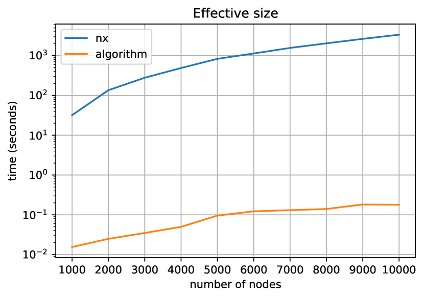
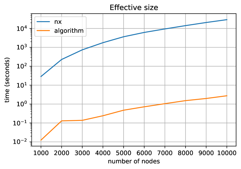
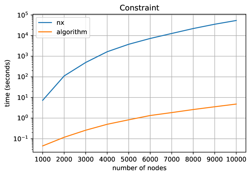
Figure 2: A basic comparison of computational speed between this paper’s algorithms (orange) and NetworkX’s algorithms (blue) for effective size (left) and constraint (right), as the number of nodes increases from 1,000 to 10,000. The networks are Barabasi-Albert graphs with parameter $m=5$ (top row) and Erdos-Renyi random graphs with parameter $p=0.01$ (bottom row). Notice, however, that a precise comparison in a controlled environment should show that more efficient methods scale better and are better suited for large networks.

In this note, I consider the main measures associated with structural holes, namely effective size, redundancy, local constraint and constraint, and derive simple formulas from the adjacency matrix of the network. This might help to interpret these measures and also produces intuitive and naive algorithms based on matrix multiplications which work fairly well on moderately large networks (see Figure 2). However, while this approach is clean and simple, it has clear limitations when the network under analysis is very large. In such a case, one should avoid storing explicitly the matrices and should preferably rely on distributed algorithms and more advanced techniques for triangle listing with vertex orderings and neighborhood markers (Chiba and Nishizeki, 1985; Li et al., 2019).

2 Notation

In what follows, matrices are denoted by capital letters (e.g. $A$, $P$) and their elements denoted by the corresponding letter with subscripts (e.g. $a_{ij}$, $p_{ij}$). Generic nodes of a network (i.e., a graph) will be indicated by $i$, $j$ or $k$. Consequently, an adjacency matrix will be indicated by $A=(a_{ij})_{i,j=1,...,n}$, where $n$ is the number of nodes and the elements $a_{ij}$ can be 0 or 1 for binary networks or generic real numbers for weighted networks.

Vectors and their elements will be respectively denoted by bold letters (e.g. $\mathbf{x}$, $\mathbf{y}$) and letters with a (single) subscript (e.g. $x_{i}$). The vector obtained by taking the diagonal elements of a square matrix $A$ is denoted by $Diag(A)$ and, analogously, the matrix that has $\mathbf{x}$ as its diagonal and 0s elsewhere is denoted by $Diag(\mathbf{x})$. The transposed of a vector or matrix is denoted by $\cdot^{T}$ (e.g. $\mathbf{x}^{T}$, $A^{T}$). Hereafter, vectors are considered as columns, that is ($n\times 1$)-matrices and their transposed as row vectors $\mathbf{x}^{T}$. Accordingly, the (matrix) multiplication of a column vector $\mathbf{x}$ times a row vector $\mathbf{y}^{T}$ will give a matrix (e.g. $\mathbf{x}\mathbf{y}^{T}\in\mathbb{R}^{n\times n}$) whereas $\mathbf{x}^{T}\mathbf{y}$ a scalar.

The matrix multiplication between two matrices $A$ and $B$ will be denoted by juxtaposition, i.e. $AB$, whereas element-by-element operations such as element-wise multiplication or division will be denoted respectively by $\odot$ and $\oslash$. The $n$-dimensional unitary vectors in $\mathbb{R}^{n}$ containing all 0s but one 1 in $i$-th position is denoted by $\mathbf{e}_{i}$, while the vector containing all 1s is denoted by $\mathbf{1}$. The identity matrix is denoted by $I$.

3 Effective size and redundancy for undirected binary networks

The original definition of effective size and redundancy in Burt’s works was complicated, but Borgatti (1997) has shown that it can be simplified. Here, we consider an undirected and binary network with no self-loops. The intuitive idea (see Figure 1) is first to compute a node’s redundancy, which is the mean number of connections from a neighbor to other neighbors. Then, the effective size is obtained by subtracting the redundancy to the node’s degree.

Let $r_{i}$ be the redundancy of node $i$ and let $t_{i}$ be “the number of ties in the network (not including ties to ego)” (Borgatti, 1997). Then, the redundancy is simply

$$r_{i}=\frac{2\ t_{i}}{d_{i}},$$ (1)

where $d_{i}$ is $i$’s degree. Notice that $r_{i}$ goes from 0 to $d_{i}-1$. Then, the effective size $s_{i}$ of node $i$ is defined as:

$$s_{i}=d_{i}-r_{i}.$$ (2)

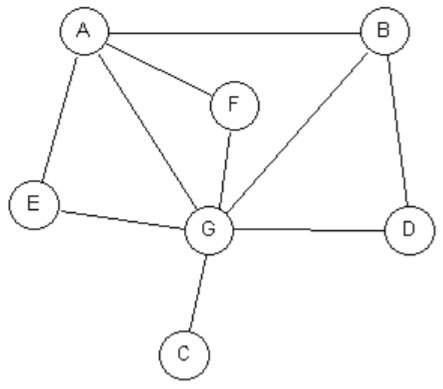
Description of redundancy and effective size

Figure 1: Adapted from Burt’s and Borgatti’s works. Let us compute the effective size for node $A$. Consider one of its neighbors, say $G$. Then, $A$ and $G$ have 3 “common neighbors”: $B$, $E$ and $F$. Analogously for all 4 neighbors of $A$ (respectively, $B$, $E$, $F$ and $G$). Summing up all these numbers and divide them by $A$’s degree, which is 4, gives: $\frac{1+1+1+3}{4}=\frac{6}{4}=1.5$. Lastly, $A$’s effective size is its degree minus its redundancy: $4-1.5=2.5$. In the example of this section, the matricial computation is also done for the remaining nodes.

Now, let us see how to compute this in a matricial form. Let $A=(a_{ij})_{i,j}$ be the adjacency matrix of such an undirected and binary network and let $\mathbf{d}=(d_{i})_{i}$ be the vector of nodes’ degrees. Notice that for a binary network, the elements of the square $A^{2}$ count the number of common neighbors. Indeed, for every two nodes $i$ and $j$, the $(i,j)$-th element of $A^{2}$ is:

$$(A^{2})_{ij} =\sum_{k=1}^{n}a_{ik}a_{kj}=|\{k:\,k\in N(i)\text{ and }k\in N(j)\}|$$ (3)

$$=\text{number of common neighbors of }i\text{ and }j,$$

since $a_{ik}$ is different from 0 if and only if $i$ and $k$ are linked and, analogously, $a_{kj}$ is different from 0 if and only if $k$ and $j$ are linked. Obviously, we only want to count the common neighbors for pairs of nodes that are actually linked in the network. To do so, it suffices to multiply $A^{2}$ element by element for $A$ itself. Lastly, we want to sum all these numbers and divide them by the corresponding degree.

Summing up, a matricial way to compute the vector of nodes’ effective size, $\mathbf{s}=(s_{i})_{i}$, is by computing the following vector:

$$\mathbf{s}=\mathbf{d}-(A^{2}\odot A)\boldsymbol{1}\oslash\mathbf{d},$$ (4)

where $A^{2}$ is $A$ squared with the standard matrix multiplication. The $i$-th component of such a vector, $s_{i}$, is node $i$’s effective size. By definition, the redundancy is just the last term, that is $\mathbf{r}=(A^{2}\odot A)\boldsymbol{1}\oslash\mathbf{d}$, where $\mathbf{r}=(r_{i})_{i}$.

Example

Consider the network in Figure 1. The adjacency matrix and the degree vector are, respectively

$$A=\begin{pmatrix}.&1&.&.&1&1&1\\ 1&.&.&1&.&.&1\\ .&.&.&.&.&.&1\\ .&1&.&.&.&.&1\\ 1&.&.&.&.&.&1\\ 1&.&.&.&.&.&1\\ 1&1&1&1&1&1&.\\ \end{pmatrix},\quad\mathbf{d}=\begin{pmatrix}4\\ 3\\ 1\\ 2\\ 2\\ 2\\ 6\end{pmatrix}.$$

Now, since

$$A^{2}=\begin{pmatrix}4&1&1&2&1&1&3\\ 1&3&1&1&2&2&2\\ 1&1&1&1&1&1&0\\ 2&1&1&2&1&1&1\\ 1&2&1&1&2&2&1\\ 1&2&1&1&2&2&1\\ 3&2&0&1&1&1&6\\ \end{pmatrix},$$

then equation (4) gives the effective size for each node:

$$\text{nodes }\left\{\begin{array}[]{c}A\\ B\\ C\\ D\\ E\\ F\\ G\\ \end{array}\right\}\quad\longrightarrow\quad\mathbf{s}=\begin{pmatrix}2.5\\ 1.667\\ 1\\ 1\\ 1\\ 1\\ 4.667\end{pmatrix}\text{ nodes' effective size}.$$

4 Local constraint (a.k.a. dyadic constraint)

Let $A=(a_{ij})_{i,j}$ be the adjacency matrix of a network (not necessarily binary or unweighted). Following Everett and Borgatti (2020), the local constraint on $i$ with respect to $j$, denoted $\ell_{ij}$, is defined by

$$\ell_{ij}=\left(p_{ij}+\sum_{k\in N(i)\setminus\{j\}}p_{ik}p_{kj}\right)^{2},$$ (5)

where $N(i)$ is the set of neighbors of $i$ and $p_{ij}$ is the normalized mutual weight of the edges joining $i$ and $j$, that is,

$$p_{ij}=\frac{a_{ij}+a_{ji}}{\sum_{k}(a_{ik}+a_{ki})}.$$ (6)

Notice that, assuming absence of self-loops, every $p_{ii}=0$, because $a_{ii}=0$. This implies that the second term in definition (5) can be written as

$$\sum_{k\in N(i)\setminus\{j\}}p_{ik}p_{kj}=\sum_{k\in N(i)}p_{ik}p_{kj}-p_{ij}\underbrace{p_{jj}}_{=0}=\sum_{k\in N(i)}p_{ik}p_{kj},$$ (7)

and, hence, $\ell_{ij}$ becomes

$$\ell_{ij}=\left(p_{ij}+\sum_{k\in N(i)}p_{ik}p_{kj}\right)^{2}.$$ (8)

Now, let us focus on $p_{ij}$, writing equation (6) in matricial terms:

$$p_{ij}=(A+A^{T})_{ij}\cdot\frac{1}{\left((A^{T}+A)\mathbf{e}_{i}\right)^{T}\mathbf{1}},$$ (9)

and let us define vector $\mathbf{x}=(x_{i})_{i}$, where

$$x_{i}=(A+A^{T})\mathbf{e}_{i}^{T}\mathbf{1}=\sum_{k}(a_{ik}+a_{ki}),$$ (10)

Thus

$$\mathbf{x}=(A+A^{T})^{T}\mathbf{1}=(A^{T}+A)\mathbf{1}$$ (11)

and we can consider the vector containing all inverted elements:

$$\mathbf{y}=\mathbf{1}\oslash\mathbf{x}=\begin{pmatrix}1/x_{1}\\ \vdots\\ 1/x_{n}.\end{pmatrix}$$ (12)

Then, define the matrix which only consists on the diagonal being equal to $\mathbf{y}$, that is, $Diag(\mathbf{y})$. Now, we can finally compute $P=(p_{ij})_{i,j}$ as follows:

$$P=Diag(\mathbf{y})\ (A+A^{T}).$$ (13)

Now, let us focus on $\ell_{ij}$. Consider again the second term of the definition’s formula as written in equation (8)

$$\sum_{k\in N(i)}p_{ik}p_{kj}=\sum_{k}a_{ik}p_{ik}p_{kj},$$ (14)

where the summation on the right-hand side is over all nodes $k$ (not just limited to $i$’s neighbors). Written in matricial form, this summation in equation (14) can simply be expressed as

$$(A\odot P)P,$$ (15)

where $\odot$ is the element-wise matricial multiplication and the second is a matrix multiplication.

To conclude, we can write the matrix $L=(\ell_{ij})_{i,j}$ containing all links’ local constraints as follows:

$$L=\big{[}P+(A\odot P)P\big{]}\odot\big{[}P+(A\odot P)P\big{]}.$$ (16)

Summing up, the algorithm takes the adjacency matrix $A$ as input and proceeds with the following steps:

1. $\mathbf{x}=(A+A^{T})\mathbf{1}$;

2. $\mathbf{y}=\mathbf{1}\oslash\mathbf{x}$;

3. $P=Diag(\mathbf{y})\ (A+A^{T})$;

4. $L=\big{[}P+(A\odot P)P\big{]}\odot\big{[}P+(A\odot P)P\big{]}$.

5 Constraint

Let $L=(\ell_{ij})_{i,j}$ be the local constraint matrix computed in equation (16). According to Everett and Borgatti (2020), the constraint for node $i$ is

$$c_{i}=\sum_{j\in N(i)}\ell_{ij}.$$

One can re-write this as follows:

$$c_{i}=\sum_{j}\ell_{ij}a_{ij},$$

where $(a_{ij})_{i,j}=A$ is the adjacency matrix. So, the vector $\mathbf{c}=(c_{i})_{i}$ containing the constraints of the network is obtained by summing the rows of the matrix $L\odot A$:

$$\mathbf{c}=\left[\mathbf{1}^{T}(L\odot A)\right]^{T}.$$

Comparison with NetworkX’s routines

References

- Bloch et al. (2019) Bloch, F., Jackson, M. O. and Tebaldi, P. (2019). Centrality measures in networks. Available at SSRN 2749124.
- Borgatti (1997) Borgatti, S. P. (1997). Structural holes: Unpacking Burt’s redundancy measures. Connections, 20 (1), 35–38.
- Burt (2004) Burt, R. S. (2004). Structural holes and good ideas. American Journal of Sociology, 110 (2), 349–399.
- Burt (2009) — (2009). Structural holes: The social structure of competition. Harvard University Press.
- Chiba and Nishizeki (1985) Chiba, N. and Nishizeki, T. (1985). Arboricity and subgraph listing algorithms. SIAM Journal on Computing, 14 (1), 210–223.
- Everett and Borgatti (2020) Everett, M. G. and Borgatti, S. P. (2020). Unpacking Burt’s constraint measure. Social Networks, 62, 50–57.
- Goyal (2018) Goyal, S. (2018). Heterogeneity and networks. In Handbook of Computational Economics, vol. 4, Elsevier, pp. 687–712.
- Goyal and Vega-Redondo (2007) — and Vega-Redondo, F. (2007). Structural holes in social networks. Journal of Economic Theory, 137 (1), 460–492.
- Granovetter (1985) Granovetter, M. (1985). Economic action and social structure: The problem of embeddedness. American Journal of Sociology, 91 (3), 481–510.
- Jackson et al. (2017) Jackson, M. O., Rogers, B. W. and Zenou, Y. (2017). The economic consequences of social-network structure. Journal of Economic Literature, 55 (1), 49–95.
- Li et al. (2019) Li, F., Zou, Z., Li, J., Li, Y. and Chen, Y. (2019). Distributed parallel structural hole detection on big graphs. In International Conference on Database Systems for Advanced Applications, Springer, pp. 519–535.
- Newman (2018) Newman, M. (2018). Networks. Oxford University Press.
- Rubí-Barceló (2017) Rubí-Barceló, A. (2017). Structural holes in social networks with exogenous cliques. Games, 8 (3), 32.
- Schweitzer et al. (2009) Schweitzer, F., Fagiolo, G., Sornette, D., Vega-Redondo, F., Vespignani, A. and White, D. R. (2009). Economic networks: The new challenges. Science, 325 (5939), 422–425.