Better Safe Than Sorry: Preventing Delusive Adversaries with Adversarial Training

Abstract

Delusive attacks aim to substantially deteriorate the test accuracy of the learning model by slightly perturbing the features of correctly labeled training examples. By formalizing this malicious attack as finding the worst-case training data within a specific $\infty$-Wasserstein ball, we show that minimizing adversarial risk on the perturbed data is equivalent to optimizing an upper bound of natural risk on the original data. This implies that adversarial training can serve as a principled defense against delusive attacks. Thus, the test accuracy decreased by delusive attacks can be largely recovered by adversarial training. To further understand the internal mechanism of the defense, we disclose that adversarial training can resist the delusive perturbations by preventing the learner from overly relying on non-robust features in a natural setting. Finally, we complement our theoretical findings with a set of experiments on popular benchmark datasets, which show that the defense withstands six different practical attacks. Both theoretical and empirical results vote for adversarial training when confronted with delusive adversaries.

1 Introduction

Although machine learning (ML) models have achieved superior performance on many challenging tasks, their performance can be largely deteriorated when the training and test distributions are different. For instance, standard models are prone to make mistakes on the adversarial examples that are considered as worst-case data at test time [10, 113]. Compared with that, a more threatening and easily overlooked threat is the malicious perturbations at training time, i.e., the delusive attacks [82] that aim to maximize test error by slightly perturbing the correctly labeled training examples [6, 7].

In the era of big data, many practitioners collect training data from untrusted sources where delusive adversaries may exist. In particular, many companies are scraping large datasets from unknown users or public websites for commercial use. For example, Kaspersky Lab, a leading antivirus company, has been accused of poisoning competing products [7]. Although they denied any wrongdoings and clarified the false rumors, one can still imagine the disastrous consequences if that really happens in the security-critical applications. Furthermore, a recent survey of 28 organizations found that these industry practitioners are obviously more afraid of data poisoning than other threats from adversarial ML [64]. In a nutshell, delusive attacks has become a realistic and horrible threat to practitioners.

Recently, Feng et al. [32] showed for the first time that delusive attacks are feasible for deep networks, by proposing “training-time adversarial data” that can significantly deteriorate model performance on clean test data. However, how to design learning algorithms that are robust to delusive attacks still remains an open question due to several crucial challenges [82, 32]. First of all, delusive attacks cannot be avoided by standard data cleaning [59], since they does not require mislabeling, and the perturbed examples will maintain their malice even when they are correctly labeled by experts. In addition, even if the perturbed examples could be distinguished by some detection techniques, it is wasteful to filter out these correctly labeled examples, considering that deep models are data-hungry. In an extreme case where all examples in the training set are perturbed by a delusive adversary, there will leave no training examples after the filtering stage, thus the learning process is still obstructed. Given these challenges, we aim to examine the following question in this study: Is it possible to defend against delusive attacks without abandoning the perturbed examples?

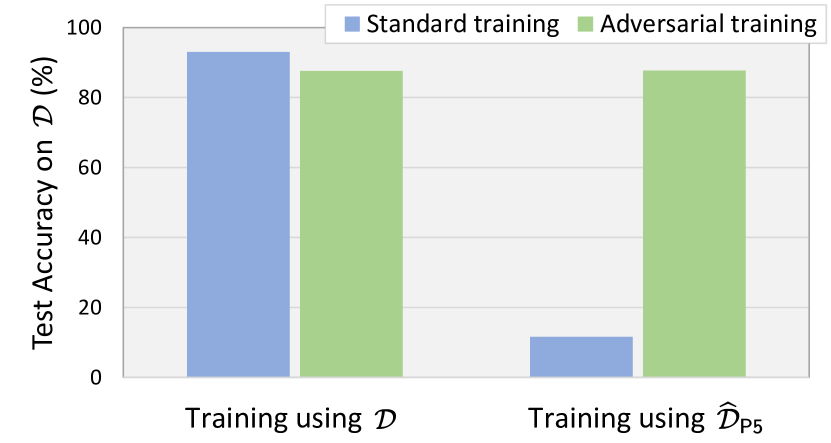
Figure 1: An illustration of delusive attacks and adversarial training. Left: Random samples from the CIFAR-10 [63] training set: the original training set $\mathcal{D}$; the perturbed training set $\widehat{\mathcal{D}}_{\mathsf{P5}}$, generated using the P5 attack described in Section 4. Right: Natural accuracy evaluated on clean test set for models trained with: i) standard training on $\mathcal{D}$; ii) adversarial training on $\mathcal{D}$; iii) standard training on $\widehat{\mathcal{D}}_{\mathsf{P5}}$; iv) adversarial training on $\widehat{\mathcal{D}}_{\mathsf{P5}}$. While standard training on $\widehat{\mathcal{D}}_{\mathsf{P5}}$ incurs poor generalization performance on $\mathcal{D}$, adversarial training can help a lot. Details are deferred to Section 5.1.

In this work, we provide an affirmative answer to this question. We first formulate the task of delusive attacks as finding the worst-case data at training time within a specific $\infty$-Wasserstein ball that prevents label changes (Section 2). By doing so, we find that minimizing the adversarial risk on the perturbed data is equivalent to optimizing an upper bound of natural risk on the original data (Section 3.1). This implies that adversarial training [44, 74] on the perturbed training examples can maximize the natural accuracy on the clean examples. Further, we disclose that adversarial training can resist the delusive perturbations by preventing the learner from overly relying on the non-robust features (that are predictive, yet brittle or incomprehensible to humans) in a simple and natural setting. Specifically, two opposite perturbation directions are studied, and adversarial training helps in both cases with different mechanisms (Section 3.2). All these evidences suggest that adversarial training is a promising solution to defend against delusive attacks.

Importantly, our findings widen the scope of application of adversarial training, which was only considered as a principled defense method against test-time adversarial examples [74, 21]. Note that adversarial training usually leads to a drop in natural accuracy [119]. This makes it less practical in many real-world applications where test-time attacks are rare and a high accuracy on clean test data is required [65]. However, this study shows that adversarial training can also defend against a more threatening and invisible threat called delusive adversaries (see Figure 1 for an illustration). We believe that adversarial training will be more widely used in practical applications in the future.

Finally, we present five practical attacks to empirically evaluate the proposed defense (Section 4). Extensive experiments on various datasets (CIFAR-10, SVHN, and a subset of ImageNet) and tasks (supervised learning, self-supervised learning, and overcoming simplicity bias) demonstrate the effectiveness and versatility of adversarial training, which significantly mitigates the destructiveness of various delusive attacks (Section 5). Our main contributions are summarized as follows:

• Formulation of delusive attacks. We provide the first attempt to formulate delusive attacks using the $\infty$-Wasserstein distance. This formulation is novel and general, and can cover the formulation of the attack proposed by Feng et al. [32].

• The principled defense. Equipped with the novel characterization of delusive attacks, we are able to show that, for the first time, adversarial training can serve as a principled defense against delusive attacks with theoretical guarantee (Theorem 1).

• Internal Mechanisms. We further disclose the internal mechanisms of the defense in a popular mixture-Gaussian setting (Theorem 2 and Theorem 3).

• Empirical evidences. We complement our theoretical findings with extensive experiments across a wide range of datasets and tasks.

2 Preliminaries

In this section, we introduce some notations and the main ideas we build upon: natural risk, adversarial risk, Wasserstein distance, and delusive attacks.

Notation. Consider a classification task with data $(\bm{x},y)\in\mathcal{X}\times\mathcal{Y}$ from an underlying distribution $\mathcal{D}$. We seek to learn a model $f:\mathcal{X}\rightarrow\mathcal{Y}$ by minimizing a loss function $\ell(f(\bm{x}),y)$. Let $\Delta:\mathcal{X}\times\mathcal{X}\rightarrow\mathbb{R}$ be some distance metric. Let $\mathcal{B}(\bm{x},\epsilon,\Delta)=\{\bm{x}^{\prime}\in\mathcal{X}:\Delta(\bm{x},\bm{x}^{\prime})\leq\epsilon\}$ be the ball around $\bm{x}$ with radius $\epsilon$. When $\Delta$ is free of context, we simply write $\mathcal{B}(\bm{x},\epsilon,\Delta)=\mathcal{B}(\bm{x},\epsilon)$. Throughout the paper, the adversary is allowed to perturb only the inputs, not the labels. Thus, similar to Sinha et al. [109], we define the cost function $c:\mathcal{Z}\times\mathcal{Z}\rightarrow\mathbb{R}\cup\{\infty\}$ by $c(\bm{z},\bm{z}^{\prime})=\Delta(\bm{x},\bm{x}^{\prime})+\infty\cdot\mathbf{1}\{y\neq y^{\prime}\}$, where $\bm{z}=(\bm{x},y)$ and $\mathcal{Z}$ is the set of possible values for $(\bm{x},y)$. Denote by $\mathcal{P}(\mathcal{Z})$ the set of all probability measures on $\mathcal{Z}$. For any $\bm{\mu}\in\mathbb{R}^{d}$ and positive definite matrix $\bm{\Sigma}\in\mathbb{R}^{d\times d}$, denote by $\mathcal{N}(\bm{\mu},\bm{\Sigma})$ the $d$-dimensional Gaussian distribution with mean vector $\bm{\mu}$ and covariance matrix $\bm{\Sigma}$.

Natural risk. Standard training (ST) aims to minimize the natural risk, which is defined as

$$\textstyle\mathcal{R}_{\mathsf{nat}}(f,\mathcal{D})=\mathbb{E}_{(\bm{x},y)\sim\mathcal{D}}\left[\ell(f(\bm{x}),y)\right].$$ (1)

The term “natural accuracy” refers to the accuracy of a model evaluated on the unperturbed data.

Adversarial risk. The goal of adversarial training (AT) is to minimize the adversarial risk defined as

$$\textstyle\mathcal{R}_{\mathsf{adv}}(f,\mathcal{D})=\mathbb{E}_{(\bm{x},y)\sim\mathcal{D}}[\max_{\bm{x}^{\prime}\in\mathcal{B}(\bm{x},\epsilon)}\ell(f(\bm{x}^{\prime}),y)],$$ (2)

which is a robust optimization problem that considers the worst-case performance under pointwise perturbations within an $\epsilon$-ball [74]. The main assumption here is that the inputs satisfying $\Delta(\bm{x},\bm{x}^{\prime})\leq\epsilon$ preserve the label $y$ of the original input $\bm{x}$.

Wasserstein distance. Wasserstein distance is a distance function defined between two probability distributions, which represents the cost of an optimal mass transportation plan. Given two data distributions $\mathcal{D}$ and $\mathcal{D}^{\prime}$, the $p$-th Wasserstein distance, for any $p\geq 1$, is defined as:

$$\textstyle\mathrm{W}_{p}(\mathcal{D},\mathcal{D}^{\prime})=(\inf_{\gamma\in\Pi(\mathcal{D},\mathcal{D}^{\prime})}\int_{\mathcal{Z}\times\mathcal{Z}}c(\bm{z},\bm{z}^{\prime})^{p}d\gamma(\bm{z},\bm{z}^{\prime}))^{1/p},$$ (3)

where $\Pi(\mathcal{D},\mathcal{D}^{\prime})$ is the collection of all probability measures on $\mathcal{Z}\times\mathcal{Z}$ with $\mathcal{D}$ and $\mathcal{D}^{\prime}$ being the marginals of the first and second factor, respectively. The $\infty$-Wasserstein distance is defined as the limit of $p$-th Wasserstein distance, i.e., $\mathrm{W}_{\infty}(\mathcal{D},\mathcal{D}^{\prime})=\lim_{p\rightarrow\infty}\mathrm{W}_{p}(\mathcal{D},\mathcal{D}^{\prime})$. The $p$-th Wasserstein ball with respect to $\mathcal{D}$ and radius $\epsilon\geq 0$ is defined as: $\mathcal{B}_{\mathrm{W}_{p}}(\mathcal{D},\epsilon)=\left\{\mathcal{D}^{\prime}\in\mathcal{P}(\mathcal{Z}):\mathrm{W}_{p}\left(\mathcal{D},\mathcal{D}^{\prime}\right)\leq\epsilon\right\}$.

Delusive adversary. The attacker is capable of manipulating the training data, as long as the training data is correctly labeled, to prevent the defender from learning an accurate classifier [82]. Following Feng et al. [32], the game between the attacker and the defender proceeds as follows:

• $n$ data points are drawn from $\mathcal{D}$ to produce a clean training dataset $\mathcal{D}_{n}$.

• The attacker perturbs some inputs $\bm{x}$ in $\mathcal{D}_{n}$ by adding small perturbations to produce $\bm{x}^{\prime}$ such that $\Delta(\bm{x},\bm{x}^{\prime})\leq\epsilon$, where $\epsilon$ is a small constant that represents the attacker’s budget. The (partially) perturbed inputs and their original labels constitute the perturbed dataset $\widehat{\mathcal{D}}_{n}$.

• The defender trains on the perturbed dataset $\widehat{\mathcal{D}}_{n}$ to produce a model, and incurs natural risk.

The attacker’s goal is to maximize the natural risk while the defender’s task is to minimize it. We then formulate the attacker’s goal as the following bi-level optimization problem:

$$\textstyle\underset{\widehat{\mathcal{D}}\in\mathcal{B}_{\mathrm{W}_{\infty}}(\mathcal{D},\epsilon)}{\max}\mathcal{R}_{\mathsf{nat}}(f_{\widehat{\mathcal{D}}},\mathcal{D}),\quad\text{ s.t. }f_{\widehat{\mathcal{D}}}=\arg\underset{f}{\min}\ \mathcal{R}_{\mathsf{nat}}(f,\widehat{\mathcal{D}}).$$ (4)

In other words, Eq. (4) is seeking the training data bounded by the $\infty$-Wasserstein ball with radius $\epsilon$, so that the model trained on it has the worst performance on the original distribution.

Remark 1. It is worth noting that using the $\infty$-Wasserstein distance to constrain delusive attacks possesses several advantages. Firstly, the cost function $c$ used in Eq. (3) prevents label changes after perturbations since we only consider clean-label attacks. Secondly, our formulation does not restrict the choice of the distance metric $\Delta$ of the input space, thus our theoretical analysis works with any metric, including the $\ell_{\infty}$ threat model considered in Feng et al. [32]. Finally, the $\infty$-Wasserstein ball is more aligned with adversarial risk than other uncertainty sets [110, 147].

Remark 2. Our formulation assumes an underlying distribution that represents the perturbed dataset. This assumption has been widely adopted by existing works [111, 118, 145]. The rationale behind the assumption is that generally, the defender treats the training dataset as an empirical distribution and trains the model on randomly shuffled examples (e.g., training deep networks via stochastic gradient descent). It is also easy to see that our formulation covers the formulation of Feng et al. [32]. On the other hand, this assumption has its limitations. For example, if the defender treats the training examples as sequential data [24], the attacker may utilize the dependence in the sequence to construct perturbations. This situation is beyond the scope of this work, and we leave it as future work.

3 Adversarial Training Beats Delusive Adversaries

In this section, we first justify the rationality of adversarial training as a principled defense method against delusive attacks in the general case for any data distribution. Further, to understand the internal mechanism of the defense, we explicitly explore the space that delusive attacks can exploit in a simple and natural setting. This indicates that adversarial training resists the delusive perturbations by preventing the learner from overly relying on the non-robust features.

3.1 Adversarial Risk Bounds Natural Risk

Intuitively, the original training data is close to the data perturbed by delusive attacks, so it should be found in the vicinity of the perturbed data. Thus, training models around the perturbed data can translate to a good generalization on the original data. We make the intuition formal in the following theorem, which indicates that adversarial training on the perturbed data is actually minimizing an upper bound of natural risk on the original data.

Theorem 1.

Given a classifier $f:\mathcal{X}\rightarrow\mathcal{Y}$, for any data distribution $\mathcal{D}$ and any perturbed distribution $\widehat{\mathcal{D}}$ such that $\widehat{\mathcal{D}}\in\mathcal{B}_{\mathrm{W}_{\infty}}(\mathcal{D},\epsilon)$, we have

$$\mathcal{R}_{\mathsf{nat}}(f,\mathcal{D})\leq\underset{\mathcal{D}^{\prime}\in\mathcal{B}_{\mathrm{W}_{\infty}}(\widehat{\mathcal{D}},\epsilon)}{\max}\mathcal{R}_{\mathsf{nat}}(f,\mathcal{D}^{\prime})=\mathcal{R}_{\mathsf{adv}}(f,\widehat{\mathcal{D}}).$$

The proof is provided in Appendix C.1. Theorem 1 suggests that adversarial training is a principled defense method against delusive attacks. Therefore, when our training data is collected from untrusted sources where delusive adversaries may exist, adversarial training can be applied to minimize the desired natural risk. Besides, Theorem 1 also highlights the importance of the budget $\epsilon$. On the one hand, if the defender is overly pessimistic (i.e., the defender’s budget is larger than the attacker’s budget), the tightness of the upper bound cannot be guaranteed. On the other hand, if the defender is overly optimistic (i.e., the defender’s budget is relatively small or even equals to zero), the natural risk on the original data cannot be upper bounded anymore by the adversarial risk. Our experiments in Section 5.1 cover these cases when the attacker’s budget is not specified.

3.2 Internal Mechanism of the Defense

To further understand the internal mechanism of the defense, in this subsection, we consider a simple and natural setting that allows us to explicitly manipulate the non-robust features. It turns out that, similar to the situation in adversarial examples [119, 56], the model’s reliance on non-robust features also allows delusive adversaries to take advantage of it, and adversarial training can resist delusive perturbations by preventing the learner from overly relying on the non-robust features.

As Ilyas et al. [56] has clarified that both robust and non-robust features in data constitute useful signals for standard classification, we are motivated to consider the following binary classification problem on a mixture of two Gaussian distributions $\mathcal{D}$:

$$y\stackrel{{\scriptstyle u\cdot a\cdot r}}{{\sim}}\{-1,+1\},\quad\bm{x}\sim\mathcal{N}(y\cdot\bm{\mu},\sigma^{2}\bm{I}),$$ (5)

where $\bm{\mu}=(1,\eta,\ldots,\eta)\in\mathbb{R}^{d+1}$ is the mean vector which consists of $1$ robust feature with center $1$ and $d$ non-robust features with corresponding centers $\eta$, similar to the settings in Tsipras et al. [119]. Typically, there are far more non-robust features than robust features (i.e., $d\gg 1$). To restrict the capability of delusive attacks, here we chose the metric function $\Delta(\bm{x},\bm{x}^{\prime})=\|\bm{x}-\bm{x}^{\prime}\|_{\infty}$. We assume that the attacker’s budget $\epsilon$ satisfies $\epsilon\geq 2\eta$ and $\eta\leq 1/3$, so that the attacker: i) can shift each non-robust feature towards becoming anti-correlated with the correct label; ii) cannot shift each non-robust feature to be strongly correlated with the correct label (as strong as the robust feature).

Delusive attack is easy. For the sake of illustration, here we choose $\epsilon=2\eta$ and consider two opposite perturbation directions. One direction is that all non-robust features shift towards $-y$, the other is to shift towards $y$. These settings are chosen for mathematical convenience. The following analysis can be easily adapted to any $\epsilon\geq 2\eta$ and any combinations of the two directions on non-robust features.

Note that the Bayes optimal classifier (i.e., minimization of the natural risk with 0-1 loss) for the distribution $\mathcal{D}$ is $f_{\mathcal{D}}(\bm{x})=\operatorname{sign}(\bm{\mu}^{\top}\bm{x})$, which relies on both robust feature and non-robust features. As a result, an $\ell_{\infty}$-bounded delusive adversary that is only allowed to perturb each non-robust feature by a moderate $\epsilon$ can take advantage of the space of non-robust features. Formally, the original distribution $\mathcal{D}$ can be perturbed to the delusive distribution $\widehat{\mathcal{D}}_{1}$:

$$\textstyle y\stackrel{{\scriptstyle u\cdot a\cdot r}}{{\sim}}\{-1,+1\},\quad\bm{x}\sim\mathcal{N}(y\cdot\widehat{\bm{\mu}}_{1},\sigma^{2}\bm{I}),$$ (6)

where $\widehat{\bm{\mu}}_{1}=(1,-\eta,\ldots,-\eta)$ is the shifted mean vector. After perturbation, every non-robust feature is correlated with $-y$, thus the Bayes optimal classifier for $\widehat{\mathcal{D}}_{1}$ would yield extremely poor performance on $\mathcal{D}$, for $d$ large enough. Another interesting perturbation direction is to strengthen the magnitude of non-robust features. This leads to the delusive distribution $\widehat{\mathcal{D}}_{2}$:

$$\textstyle y\stackrel{{\scriptstyle u\cdot a\cdot r}}{{\sim}}\{-1,+1\},\quad\bm{x}\sim\mathcal{N}(y\cdot\widehat{\bm{\mu}}_{2},\sigma^{2}\bm{I}),$$ (7)

where $\widehat{\bm{\mu}}_{2}=(1,3\eta,\ldots,3\eta)$ is the shifted mean vector. Then, the Bayes optimal classifier for $\widehat{\mathcal{D}}_{2}$ will overly rely on the non-robust features, thus likewise yielding poor performance on $\mathcal{D}$.

The above two attacks are legal because the delusive distributions are close enough to the original distribution, that is, $\mathrm{W}_{\infty}(\mathcal{D},\widehat{\mathcal{D}}_{1})\leq\epsilon$ and $\mathrm{W}_{\infty}(\mathcal{D},\widehat{\mathcal{D}}_{2})\leq\epsilon$. Meanwhile, the attacks are also harmful. The following theorem directly compares the destructiveness of the attacks.

Theorem 2.

Let $f_{\mathcal{D}}$, $f_{\widehat{\mathcal{D}}_{1}}$, and $f_{\widehat{\mathcal{D}}_{2}}$ be the Bayes optimal classifiers for the mixture-Gaussian distributions $\mathcal{D}$, $\widehat{\mathcal{D}}_{1}$, and $\widehat{\mathcal{D}}_{2}$, defined in Eqs. (5), (6), and (7), respectively. For any $\eta>0$, we have

$$\mathcal{R}_{\mathsf{nat}}(f_{\mathcal{D}},\mathcal{D})<\mathcal{R}_{\mathsf{nat}}(f_{\widehat{\mathcal{D}}_{2}},\mathcal{D})<\mathcal{R}_{\mathsf{nat}}(f_{\widehat{\mathcal{D}}_{1}},\mathcal{D}).$$

The proof is provided in Appendix C.2. Theorem 2 indicates that both attacks will increase the natural risk of the Bayes optimal classifier. Moreover, $\widehat{\mathcal{D}}_{1}$ is more harmful because it always incurs higher natural risk than $\widehat{\mathcal{D}}_{2}$. The destructiveness depends on the dimension of non-robust features. For intuitive understanding, we plot the natural accuracy of the classifiers as a function of $d$ in Figure 2. We observe that, as the number of non-robust features increases, the natural accuracy of the standard model $f_{\widehat{\mathcal{D}}_{1}}$ continues to decline, while the natural accuracy of $f_{\widehat{\mathcal{D}}_{2}}$ first decreases and then increases.

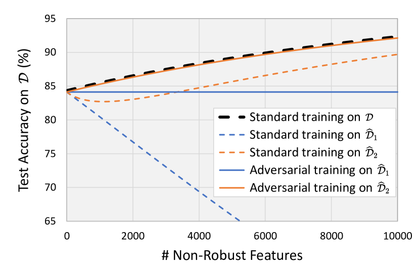
Figure 2: The natural accuracy of five models trained on the mixture-Gaussian distributions as a function of the number of non-robust features. As a concrete example, here we set $\sigma=1$, $\eta=0.01$ and vary $d$.

Adversarial training matters. Adversarial training with proper $\epsilon$ will mitigate the reliance on non-robust features. For $\widehat{\mathcal{D}}_{1}$ the internal mechanism is similar to the case in Tsipras et al. [119], while for $\widehat{\mathcal{D}}_{2}$ the mechanism is different, and there was no such analysis before. Specifically, the optimal linear $\ell_{\infty}$ robust classifier (i.e., minimization of the adversarial risk with 0-1 loss) for $\widehat{\mathcal{D}}_{1}$ will rely solely on the robust feature. In contrast, the optimal robust classifier for $\widehat{\mathcal{D}}_{2}$ will rely on both robust and non-robust features, but the excessive reliance on non-robust features is mitigated. Hence, adversarial training matters in both cases and achieves better natural accuracy when compared with standard training. We make this formal in the following theorem.

Theorem 3.

Let $f_{\widehat{\mathcal{D}}_{1},\mathsf{rob}}$ and $f_{\widehat{\mathcal{D}}_{2},\mathsf{rob}}$ be the optimal linear $\ell_{\infty}$ robust classifiers for the delusive distributions $\widehat{\mathcal{D}}_{1}$ and $\widehat{\mathcal{D}}_{2}$, defined in Eqs. (6) and (7), respectively. For any $0<\eta<1/3$, we have

$$\mathcal{R}_{\mathsf{nat}}(f_{\widehat{\mathcal{D}}_{1}},\mathcal{D})>\mathcal{R}_{\mathsf{nat}}(f_{\widehat{\mathcal{D}}_{1},\mathsf{rob}},\mathcal{D})\quad\text{and}\quad\mathcal{R}_{\mathsf{nat}}(f_{\widehat{\mathcal{D}}_{2}},\mathcal{D})>\mathcal{R}_{\mathsf{nat}}(f_{\widehat{\mathcal{D}}_{2},\mathsf{rob}},\mathcal{D}).$$

The proof is provided in Appendix C.3. Theorem 3 indicates that robust models achieve lower natural risk than standard models under delusive attacks. This is also reflected in Figure 2: After adversarial training on $\widehat{\mathcal{D}}_{1}$, natural accuracy is largely recovered and keeps unchanged as $d$ increases. While on $\widehat{\mathcal{D}}_{2}$, natural accuracy can be recovered better and keeps increasing as $d$ increases. Beyond the theoretical analyses for these simple cases, we also observe that the phenomena in Theorem 2 and Theorem 3 generalize well to our empirical experiments on real-world datasets in Section 5.1.

4 Practical Attacks for Testing Defense

Here we briefly describe five heuristic attacks. A detailed description is deferred to Appendix D. The five attacks along with the L2C attack proposed by Feng et al. [32] will be used in next section for validating the destructiveness of delusive attacks and thus the necessity of adversarial training.

In practice, we focus on the empirical distribution $\mathcal{D}_{n}$ over $n$ data points drawn from $\mathcal{D}$. Inspired by “non-robust features suffice for classification” [56], we propose to construct delusive perturbations by injecting non-robust features correlated consistently with a specific label. Given a standard model $f_{\mathcal{D}}$ trained on $\mathcal{D}_{n}$, the attacks perturb each input $\bm{x}$ (with label $y$) in $\mathcal{D}_{n}$ as follows:

• P1: Adversarial perturbations. It adds a small adversarial perturbation to $\bm{x}$ to ensure that it is misclassified as a target $t$ by minimizing $\ell\left(f_{\mathcal{D}}(\bm{x}^{\prime}),t\right)$ such that $\bm{x}^{\prime}\in\mathcal{B}(\bm{x},\epsilon)$, where $t$ is chosen deterministially based on $y$.

• P2: Hypocritical perturbations. It adds a small helpful perturbation to $\bm{x}$ by minimizing $\ell\left(f_{\mathcal{D}}(\bm{x}^{\prime}),y\right)$ such that $\bm{x}^{\prime}\in\mathcal{B}(\bm{x},\epsilon)$, so that the standard model could easily produce a correct prediction.

• P3: Universal adversarial perturbations. This attack is a variant of P1. It adds the class-specific universal adversarial perturbation $\bm{\xi}_{t}$ to $\bm{x}$. All inputs with the same label $y$ are perturbed with the same perturbation $\bm{\xi}_{t}$, where $t$ is chosen deterministially based on $y$.

• P4: Universal hypocritical perturbations. This attack is a variant of P2. It adds the class-specific universal helpful perturbation $\bm{\xi}_{y}$ to $\bm{x}$. All inputs with the same label $y$ are perturbed with the same perturbation $\bm{\xi}_{y}$.

• P5: Universal random perturbations. This attack injects class-specific random perturbation $\bm{r}_{y}$ to each $\bm{x}$. All inputs with the label $y$ is perturbed with the same perturbation $\bm{r}_{y}$. Despite the simplicity of this attack, we find that it are surprisingly effective in some cases.

Figure 3 visualizes the universal perturbations for different datasets and threat models. The perturbed inputs and their original labels constitute the perturbed datasets $\widehat{\mathcal{D}}_{\mathsf{P1}}\sim\widehat{\mathcal{D}}_{\mathsf{P5}}$.

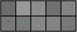
(a) CIFAR-10 ($\ell_{2}$)

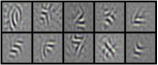
(b) SVHN ($\ell_{2}$)

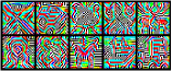
(c) CIFAR-10 ($\ell_{\infty}$)

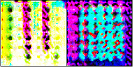
(d) ImageNet ($\ell_{\infty}$)

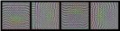
(e) SSL ($\ell_{2}$)

Figure 3: Universal perturbations for the P3 and P4 attacks across different datasets and threat models. Perturbations are rescaled to lie in the $[0,1]$ range for display. The resulting inputs are nearly indistinguishable from the originals to a human observer (see Appendix B Figures 10, 11, and 12).

5 Experiments

In order to demonstrate the effectiveness and versatility of the proposed defense, we conduct experiments on CIFAR-10 [63], SVHN [81], a subset of ImageNet [95], and MNIST-CIFAR [104] datasets. More details on experimental setup are provided in Appendix A. Our code is available at https://github.com/TLMichael/Delusive-Adversary.

Firstly, we perform a set of experiments on supervised learning to provide a comprehensive understanding of delusive attacks (Section 5.1). Secondly, we demonstrate that the delusive attacks can also obstruct rotation-based self-supervised learning (SSL) [41] and adversarial training also helps a lot in this case (Section 5.2). Finally, we show that adversarial training is a promising method to overcome the simplicity bias on the MNIST-CIFAR dataset [104] if the $\epsilon$-ball is chosen properly (Section 5.3).

5.1 Understanding Delusive Attacks

Here, we investigate delusive attacks from six different perspectives: i) baseline results on CIFAR-10, ii) transferability of delusive perturbations to various architectures, iii) performance changes of various defender’s budgets, iv) a simple countermeasure, v) comparison with Feng et al. [32], and vi) performance of other adversarial training variants.

Baseline results. We consider the typical $\ell_{2}$ threat model with $\epsilon=0.5$ for CIFAR-10 by following [56]. We use the attacks described in Section 4 to generate the delusive perturbations. To execute the attacks P1 $\sim$ P4, we pre-train a VGG-16 [108] as the standard model $f_{\mathcal{D}}$ using standard training on the original training set. We then perform standard training and adversarial training on the delusive datasets $\widehat{\mathcal{D}}_{\mathsf{P1}}\sim\widehat{\mathcal{D}}_{\mathsf{P5}}$. Standard data augmentation (i.e., cropping, mirroring) is adopted. The natural accuracy of the models is evaluated on the clean test set of CIFAR-10.

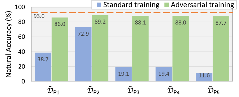
Figure 4: Natural accuracy on CIFAR-10 using VGG-16 under $\ell_{2}$ threat model. The horizontal line indicates the natural accuracy of a standard model trained on the clean training set.

Results are summarized in Figure 4. We observe that the natural accuracy of the standard models dramatically decreases when training on the delusive datasets, especially on $\widehat{\mathcal{D}}_{\mathsf{P3}}$, $\widehat{\mathcal{D}}_{\mathsf{P4}}$ and $\widehat{\mathcal{D}}_{\mathsf{P5}}$. The most striking observation to emerge from the results is the effectiveness of the P5 attack. It seems that the naturally trained model seems to rely exclusively on the small random patterns in this case, even though there are still abundant natural features in $\widehat{\mathcal{D}}_{\mathsf{P5}}$. Such behaviors resemble the conjunction learner studied in the pioneering work [82], where they showed that such a learner is highly vulnerable to delusive attacks. Also, we point out that such behaviors could be attributed to the gradient starvation [91] and simplicity bias [104] phenomena of neural networks. These recent studies both show that neural networks trained by SGD preferentially capture a subset of features relevant for the task, despite the presence of other predictive features that fail to be discovered [50].

Anyway, our results demonstrate that adversarial training can successfully eliminate the delusive features within the $\epsilon$-ball. As shown in Figure 4, natural accuracy can be significantly improved by adversarial training in all cases. Besides, we observe that P1 is more destructive than P2, which is consistent with our theoretical analysis of the hypothetical settings in Section 3.2.

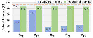
(a) VGG-19

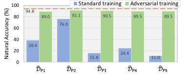
(b) ResNet-18

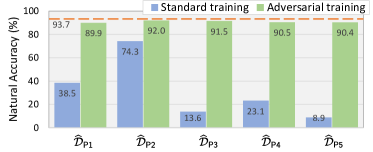
(c) ResNet-50

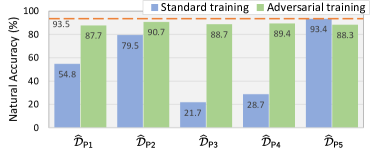
(d) DenseNet-121

Figure 8: Natural accuracy on CIFAR-10 under $\ell_{2}$ threat model. The horizontal orange line indicates the natural accuracy of a standard model trained on the clean training set.

Evaluation of transferability. A more realistic setting is to attack different classifiers using the same delusive perturbations. We consider various architectures including VGG-19, ResNet-18, ResNet-50, and DenseNet-121 as victim classifiers. The delusive datasets are the same as in the baseline experiments. Results are deferred to Figure 8 in Appendix B. We observe that the attacks have good transferability across the architectures, and again, adversarial training can substantially improve natural accuracy in all cases. One exception is that the P5 attack is invalid for DenseNet-121. A possible explanation for this might be that the simplicity bias of DenseNet-121 on random patterns is minor. This means that different architectures may have distinct simplicity biases. Due to space constraints, a detailed investigation is out of the scope of this work.

What if the threat model is not specified? Our theoretical analysis in Section 3.1 highlights the importance of choosing a proper budget $\epsilon$ for AT. Here, we try to explore this situation where the threat model is not specified by varying the defender’s budget. Results on CIFAR-10 using ResNet-18 under $\ell_{2}$ threat model are summarized in Figure 6. We observe that a budget that is too large may slightly hurt performance, while a budget that is too small is not enough to mitigate the attacks. Empirically, the optimal budget for P3 and P4 is about $0.4$ and for P1 and P2 it is about $0.25$. P5 is the easiest to defend—AT with a small budget (about $0.1$) can significantly mitigate its effect.

A simple countermeasure. In addition to adversarial training, a simple countermeasure is adding clean data to the training set. This will neutralize the perturbed data and make it closer to the original distribution. We explore this countermeasure on SVHN since extensive extra training examples are available in that dataset. Results are summarized in Figure 6. We observe that the performance of standard training is improved with the increase of the number of additional clean examples, and the performance of adversarial training can also be improved with more data. Overall, it is recommend that combining this simple countermeasure with adversarial training to further improve natural accuracy. Besides the focus on natural accuracy in this work, another interesting measure is the model accuracy on adversarial examples. It turns out that adversarial accuracy of the models can also be improved with more data. We also observe that different delusive attacks have different effects on the adversarial accuracy. A further study with more focus on adversarial accuracy is therefore suggested.

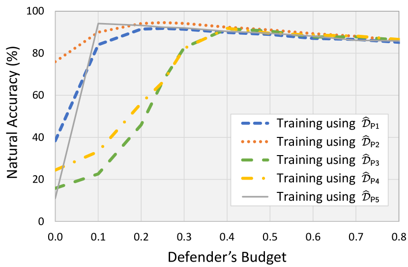
Figure 5: Natural accuracy as a function of the defender’s budget on CIFAR-10.

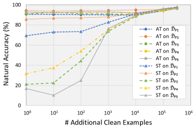
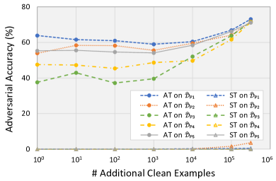
Figure 6: Natural accuracy (left) and adversarial accuracy (right) as a function of the number of additional clean examples on SVHN using ResNet-18 under $\ell_{2}$ threat model.

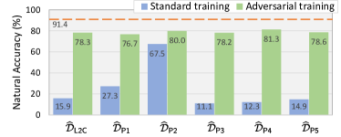
(a) CIFAR-10

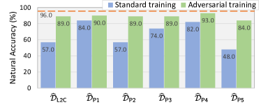
(b) Two-class ImageNet

Figure 7: Natural accuracy on CIFAR-10 using VGG-11 (left) and two-class ImageNet using ResNet-18 (right) under $\ell_{\infty}$ threat model. The horizontal orange line indicates the natural accuracy of a standard model trained on the clean training set.

Table 1: Comparison of time cost. The L2C attack needs to train an autoencoder to generate perturbations. The P1 $\sim$ P4 attacks need to train a standard classifier to generate perturbations, and P5 needs not.

Method	Time Cost (min)
	Training	Generating	Total
L2C	7411.5	0.4	7411.9
P1 / P2	25.9	12.6	38.5
P3 / P4	25.9	4.6	30.5
P5	0.0	0.1	0.1

Comparison with L2C. We compare the heuristic attacks with the L2C attack proposed by Feng et al. [32] and, show that adversarial training can mitigate all these attacks. Following their settings on CIFAR-10 and a two-class ImageNet, the $\ell_{\infty}$-norm bounded threat models with $\epsilon=0.032$ and $\epsilon=0.1$ are considered. The victim classifier is VGG-11 and ResNet-18 for CIFAR-10 and the two-class ImageNet, respectively. Table 1 reports the time cost for executing six attack methods on CIFAR-10. We find that the heuristic attacks are significantly faster than L2C, since the bi-level optimization process in L2C is extremely time-consuming. Figure 7 shows the performance of standard training and adversarial training on delusive datasets. The results indicate that most of the heuristic attacks are comparable with L2C, and AT can improve natural accuracy in all cases.

Performance of adversarial training variants. It is noteworthy that AT variants are also effective in our setting, since they aim to tackle the adversarial risk. To support this, we consider instance-dependent-based variants (such as MART [125], GAIRAT [141], and MAIL [123]) and curriculum-based variants (such as CAT [13], DAT [124], FAT [140]). Specifically, we chose to experiment with the currently most effective variants among them (i.e., GAIRAT and FAT, according to the latest leaderboard at RobustBench [21]). Additionally, we consider random noise training (denoted as RandNoise) using the uniform noise within the $\epsilon$-ball for comparison. We also report the results of standard training (denoted as ST) and the conventional PGD-based AT [74] (denoted as PGD-AT) for reference. The results are summarized in Table 2. We observe that the performance of random noise training is marginal. In contrast, all AT methods show significant improvements, thanks to the theoretical analysis provided by Theorem 1. Besides, we observe that FAT achieves overall better results than other AT variants. This may be due to the tight upper bound of the adversarial risk pursued by FAT. In summary, these results successfully validate the effectiveness of AT variants.

Table 2: Natural accuracy on CIFAR-10 using ResNet-18 under $\ell_{\infty}$ threat model with $\epsilon=8/255$. The column of “Clean” denotes the natural accuracy of the models trained on the clean training set.

Method	Clean	L2C	P1	P2	P3	P4	P5
ST	94.62	15.76	15.70	61.35	9.40	13.58	10.12
RandNoise	94.26	17.10	17.32	63.36	10.52	14.37	27.56
PGD-AT	85.18	82.84	84.18	86.74	86.37	83.18	84.57
GAIRAT	81.90	79.96	79.61	82.68	82.05	82.81	82.28
FAT	87.43	85.51	86.05	88.98	84.39	84.22	87.78

Table 3: Adversarial training on MNIST-CIFAR: The table reports test accuracy on the MNIST-CIFAR test set and the MNIST-randomized test set. Our customized AT successfully overcomes SB, while others not. The MNIST-randomized accuracy indicates that our adversarially trained models achieve nontrivial performance when there are only CIFAR features exist in the inputs.

Model	Test Accuracy on MNIST-CIFAR			MNIST-Randomized Accuracy
	ST	AT [104]	AT (ours)	ST	AT [104]	AT (ours)
VGG-16	99.9	100.0	91.3	49.1	51.6	91.2
ResNet-50	100.0	99.9	89.7	48.9	49.2	88.6
DenseNet-121	100.0	100.0	91.5	48.8	49.2	90.8

5.2 Evaluation on Rotation-based Self-supervised Learning

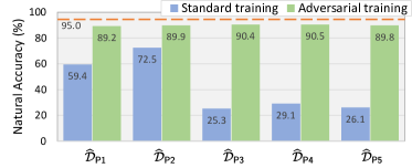
(a) Pretext task

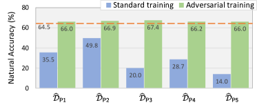
(b) Downstream task

Figure 9: Rotation-based SSL on CIFAR-10 using ResNet-18 under $\ell_{2}$ threat model. The horizontal line indicates the natural accuracy of a standard model trained on the clean training set.

To further show the versatility of the attacks and defense, we conduct experiments on rotation-based self-supervised learning (SSL) [41], a process that learns representations by predicting rotation angles ($0^{\circ}$, $90^{\circ}$, $180^{\circ}$, $270^{\circ}$). SSL methods seem to be inherently resist to the poisoning attacks that require mislabeling, since they do not use human-annotated labels to learn representations. Here, we examine whether SSL can resist the delusive attacks. We use delusive attacks to perturb the training data for the pretext task. To evaluate the quality of the learned representations, the downstream task is trained on the clean data using logistic regression. Results are deferred to Figure 9 in Appendix B.

We observe that the learning of the pretext task can be largely hijacked by the attacks. Thus the learned representations are poor for the downstream task. Again, adversarial training can significantly improve natural accuracy in all cases. An interesting observation from Figure 9(b) is that the quality of the adversarially learned representations is slightly better than that of standard models trained on the original training set. This is consistent with recent hypotheses stating that robust models may transfer better [98, 121, 69, 22, 2]. These results show the possibility of delusive attacks and defenses for SSL, and suggest that studying the robustness of other SSL methods [58, 17] against data poisoning is a promising direction for future research.

5.3 Overcoming Simplicity Bias

A recent work by Shah et al. [104] proposed the MNIST-CIFAR dataset to demonstrate the simplicity bias (SB) of using standard training to learn neural networks. Specifically, the MNIST-CIFAR images $\bm{x}$ are vertically concatenations of the “simple” MNIST images $\bm{x}_{m}$ and the more complex CIFAR-10 images $\bm{x}_{c}$ (i.e., $\bm{x}=[\bm{x}_{m};\bm{x}_{c}]$). They found that standard models trained on MNIST-CIFAR will exclusively rely on the MNIST features and remain invariant to the CIFAR features. Thus randomizing the MNIST features drops the model accuracy to random guessing.

From the perspective of delusive adversaries, we can regard the MNIST-CIFAR dataset as a delusive version of the original CIFAR dataset. Thus, AT should mitigate the delusive perturbations, as Theorem 1 pointed out. However, Shah et al. [104] tried AT on MNIST-CIFAR yet failed. Contrary to their results, here we demonstrate that AT is actually workable. The key factor is the choice of the threat model. They failed because they chose an improper ball $\mathcal{B}(\bm{x},\epsilon)=\{\bm{x}^{\prime}\in\mathcal{X}:\|\bm{x}-\bm{x}^{\prime}\|_{\infty}\leq 0.3\}$, while we set $\mathcal{B}(\bm{x},\epsilon)=\{\bm{x}^{\prime}\in\mathcal{X}:\|\bm{x}_{m}-\bm{x}_{m}^{\prime}\|_{\infty}+\infty\cdot\|\bm{x}_{c}-\bm{x}_{c}^{\prime}\|_{\infty}\leq 1\}$. Our choice forces the space of MNIST features to be a non-robust region during AT, and prohibits the CIFAR features from being perturbed. Results are summarized in Table 3. We observe that our choice leads to models that do not rely on the simple MNIST features, thus AT can eliminate the simplicity bias.

6 Related Work

Data poisoning. The main focus of this paper is the threat of delusive attacks [82], which belongs to data poisoning attacks [6, 7, 43]. Generally speaking, data poisoning attacks manipulate the training data to cause a model to fail during inference. Both integrity and availability attacks were extensively studied for classical models [5, 42, 82, 80, 8, 9, 76, 132, 143]. For neural networks, most of the existing works focused on targeted misclassification [61, 103, 145, 1, 55, 39, 105, 20, 92] and backdoor attacks [47, 18, 71, 120, 72, 83, 86, 84], while there was little work on availability attacks [102, 78, 32, 106]. Recently, Feng et al. [32] showed that availability attacks are feasible for deep networks. This paper follows their setting where the perturbed training data is correctly labeled. We further point out that their studied threat is exactly the delusive adversary (a.k.a. clean-label availability attacks), which was previously considered for classical models [82]. Besides, other novel directions of data poisoning are rapidly evolving such as semi-supervised learning [70, 35, 14], contrastive learning [15, 96], domain adaptation [75], and online learning [88], etc.

Existing defenses. There were many defense strategies proposed for defending against targeted attacks and backdoor attacks, including detection-based defenses [111, 118, 16, 23, 38, 90, 48, 28], randomized smoothing [94, 127], differential privacy [73, 51], robust training [12, 66, 67, 40], and model repairing [19, 68, 130], while some of them may be overwhelmed by adaptive attacks [62, 122, 107]. Robust learnability under data poisoning attacks can be analyzed from theoretical aspects [11, 126, 36]. Similarly, our proposed defense is principled and theoretically justified. More importantly, previous defenses mostly focus on defending against integrity attacks, while none of them are specially designed to resist delusive attacks. The work most similar to ours is that of Farokhi [31]. They only handle the linear regression model by relaxing distributionally robust optimization (DRO) as a regularizer, while we can tackle delusive attacks for any classifier.

Adversarial training. Since the discovery of adversarial examples (a.k.a. evasion attacks at test time) in neural networks [10, 113], plenty of defense methods have been proposed to mitigate this vulnerability [44, 89, 3]. Among them, adversarial training is practically considered as a principled defense against test-time adversarial examples [74, 21] at the price of slightly worse natural accuracy [112, 119, 135] and moderate robust generalization [101, 93], and many variants were devoted to improving the performance [139, 140, 26, 131, 87, 37, 29, 114, 54, 45, 27]. Besides, it has been found that adversarial training may intensify backdoor attacks in experiments [128]. In contrast, both of our theoretical and empirical evidences suggest that adversarial training can mitigate delusive attacks. On the other hand, adversarial training also led to further benefits in robustness to noisy labels [146], out-of-distribution generalization [133, 136, 60], transfer learning [98, 116, 121], domain adaption [4], novelty detection [46, 97], explainability [142, 85], and image synthesis [100].

Concurrent work. The threat of delusive attacks [82, 32] is attracting attention from the community. Several attack techniques are concurrently and independently proposed, including Unlearnable Examples [53], Alignment [33], NTGA [137], Adversarial Shortcuts [30], and Adversarial Poisoning [34]. Contrary to them, we mainly focus on introducing a principled defense method (i.e., adversarial training), while as by-products, five delusive attacks are presented and investigated in this paper. Meanwhile, Huang et al. [53] and Fowl et al. [34] also experiment with adversarial training, but only for their proposed delusive attacks. In contrast, this paper not only provides empirical evidence on the success of adversarial training against six different delusive attacks, but also offers theoretical justifications for the defense, which is of great significance to security. We believe that our findings will promote the use of adversarial training in practical applications in the future.

7 Conclusion and Future Work

In this paper, we suggest applying adversarial training in practical applications, rather than standard training whose performance risks being substantially deteriorated by delusive attacks. Both theoretical and empirical results vote for adversarial training when confronted with delusive adversaries. Nonetheless, some limitations remain and may lead to future directions: i) Our implementation of adversarial training adopts the popular PGD-AT framework [74, 87], which could be replaced with certified training methods [129, 138] for better robustness guarantee. ii) The success of our proposed defense relies on generalization, just like most ML algorithms, so an analysis of robust generalization error bound for this case would be useful. iii) Adversarial training may increase the disparity of accuracy between groups [134, 117], which could be mitigated by fair robust learning [134].

Supplementary Material:

Better Safe Than Sorry: Preventing Delusive Adversaries with Adversarial Training

Appendix A Experimental Setup

Experiments run with NVIDIA GeForce RTX 2080 Ti GPUs. We report the number with a single run of experiments. Our implementation is based on PyTorch, and the code to reproduce our results is available at https://github.com/TLMichael/Delusive-Adversary.

A.1 Datasets and Models

Table 4 reports the parameters used for the datasets and models.

CIFAR-10.  This dataset [63] consists of 60,000 $32\times 32$ colour images (50,000 images for training and 10,000 images for testing) in 10 classes (“airplane”, “car”, “bird”, “cat”, “deer”, “dog”, “frog”, “horse”, “ship”, and “truck”). Early stopping is done with holding out 1000 examples from the training set. We use various architectures for this dataset, including VGG-11, VGG-16, VGG-19 [108], ResNet-18, ResNet-50 [49], and DenseNet-121 [52]. The initial learning rate is set to 0.1. For supervised learning on this dataset, we run 150 epochs on the training set, where we decay the learning rate by a factor 0.1 in the 100th and 125th epochs. For self-supervised learning, we run 70 epochs, where we decay the learning rate by a factor 0.1 in the 40th and 55th epochs. The license for this dataset is unknown.

SVHN.  This dataset [81] consists of 630,420 $32\times 32$ colour images (73,257 images for training, 26,032 images for testing, and 531,131 additional images to use as extra training data) in 10 classes (“0”, “1”, “2”, “3”, “4”, “5”, “6”, “7”, “8”, and “9”). Early stopping is done with holding out 1000 examples from the training set. We use the ResNet-18 architecture for this dataset. The initial learning rate is set to 0.01. We run 50 epochs on the training set, where we decay the learning rate by a factor 0.1 in the 30th and 40th epochs. The license for this dataset is custom (non-commercial).

Two-class ImageNet.  Following Feng et al. [32], this dataset is a subset of ImageNet [95] that consists of 2,700 $224\times 224$ colour images (2,600 images for training and 100 images for testing) in 2 classes (“bulbul”, “jellyfish”). Early stopping is done with holding out 380 examples from the training set. We use the ResNet-18 architecture for this dataset. The initial learning rate is set to 0.1. We run 100 epochs on the training set, where we decay the learning rate by a factor 0.1 in the 75th and 90th epochs. The license for this dataset is custom (research, non-commercial).

MNIST-CIFAR.  Following Shah et al. [104], this dataset consists of 11,960 $64\times 32$ colour images (10,000 images for training and 1,960 images for testing) in 2 classes: images in class $-1$ and class $1$ are vertical concatenations of MNIST digit zero & CIFAR-10 car and MNIST digit one & CIFAR-10 truck images, respectively. We use various architectures for this dataset, including VGG-16, ResNet-50, and DenseNet-121. The initial learning rate is set to 0.05. We run 100 epochs on the training set, where we decay the learning rate by a factor 0.2 in the 50th and 150th epochs and a factor 0.5 in the 100th epoch. The license for this dataset is unknown.

Parameter	CIFAR-10	SVHN	Two-class ImageNet	MNIST-CIFAR
# training examples	50,000	73,257	2,600	10,000
# test examples	10,000	26,032	100	1,960
# features	3,072	3,072	150,528	6,144
# classes	10	10	2	2
batch size	128	128	32	256
learning rate	0.1	0.01	0.1	0.05
SGD momentum	0.9	0.9	0.9	0.9
weight decay	$5\cdot 10^{-4}$	$5\cdot 10^{-4}$	$5\cdot 10^{-4}$	$5\cdot 10^{-5}$

Table 4: Experimental setup and parameters for the each dataset.

A.2 Adversarial Training

Unless otherwise specified, we perform adversarial training to train robust classifiers by following Madry et al. [74]. Specifically, we train against a projected gradient descent (PGD) adversary, starting from a random initial perturbation of the training data. We consider adversarial perturbations in $\ell_{p}$ norm where $p=\{2,\infty\}$. Unless otherwise specified, we use the values of $\epsilon$ provided in Table 5 to train our models. We use 7 steps of PGD with a step size of $\epsilon/5$. For overcoming simplicity bias on MNIST-CIFAR, we modify the original $\epsilon$-ball used in Shah et al. [104] (i.e., $\mathcal{B}(\bm{x},\epsilon)=\{\bm{x}^{\prime}\in\mathcal{X}:\|\bm{x}-\bm{x}^{\prime}\|_{\infty}\leq 0.3\}$) to the entire space of the MNIST features $\mathcal{B}(\bm{x},\epsilon)=\{\bm{x}^{\prime}\in\mathcal{X}:\|\bm{x}_{m}-\bm{x}_{m}^{\prime}\|_{\infty}+\infty\cdot\|\bm{x}_{c}-\bm{x}_{c}^{\prime}\|_{\infty}\leq 1\}$, where $\bm{x}$ represents the vertical concatenation of a MNIST image $\bm{x}_{m}$ and a CIFAR-10 image $\bm{x}_{c}$.

Adversary	CIFAR-10	SVHN	Two-class ImageNet
$\ell_{\infty}$	0.032	-	0.1
$\ell_{2}$	0.5	0.5	-

Table 5: Value of $\epsilon$ used for adversarial training of each dataset and $\ell_{p}$ norm.

A.3 Delusive Adversaries

Six delusive attacks are considered to validate our proposed defense. We reimplement the L2C attack [32] using the code provided by the authors. The other five attacks are constructed as follows. To execute P1 $\sim$ P4, we perform normalized gradient descent ($\ell_{p}$-norm of gradient is fixed to be constant at each step). At each step we clip the input to in the $[0,1]$ range so as to ensure that it is a valid image. To execute P5, noises are sampled from Gaussian distribution and then projected to the ball for $\ell_{2}$-norm bounded perturbations; for $\ell_{\infty}$-norm bounded perturbations, noises are directly sampled from a uniform distribution. Unless otherwise specified, the attacker’s $\epsilon$ are the same with adversarial training used by the defender. Details on the optimization procedure are shown in Table 6.

Parameter	P1	P2	P3	P4	P5
step size	$\epsilon/5$	$\epsilon/5$	$\epsilon/5$	$\epsilon/5$	$\epsilon$
iterations	100	100	500	500	1

Table 6: Parameters used for optimization procedure to construct each delusive dataset in Section 4.

Appendix B Omitted Figures

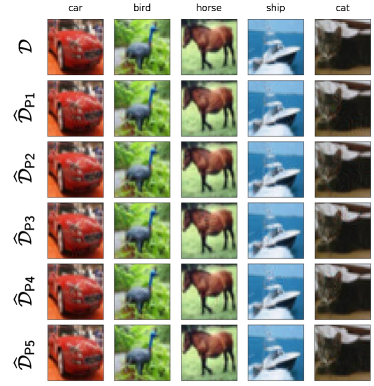
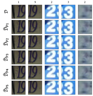
Figure 10: Left: Random samples from the CIFAR-10 training set: the original training $\mathcal{D}$; the perturbed training sets $\widehat{\mathcal{D}}_{\mathsf{P1}}$, $\widehat{\mathcal{D}}_{\mathsf{P2}}$, $\widehat{\mathcal{D}}_{\mathsf{P3}}$, $\widehat{\mathcal{D}}_{\mathsf{P4}}$, and $\widehat{\mathcal{D}}_{\mathsf{P5}}$. The threat model is the $\ell_{2}$ ball with $\epsilon=0.5$. Right: First five examples from the SVHN training set: the original training $\mathcal{D}$; the perturbed training sets $\widehat{\mathcal{D}}_{\mathsf{P1}}$, $\widehat{\mathcal{D}}_{\mathsf{P2}}$, $\widehat{\mathcal{D}}_{\mathsf{P3}}$, $\widehat{\mathcal{D}}_{\mathsf{P4}}$, and $\widehat{\mathcal{D}}_{\mathsf{P5}}$. The threat model is the $\ell_{2}$ ball with $\epsilon=0.5$.

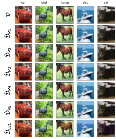
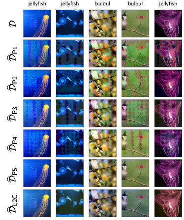
Figure 11: Left: Random samples from the CIFAR-10 training set: the original training $\mathcal{D}$; the perturbed training sets $\widehat{\mathcal{D}}_{\mathsf{P1}}$, $\widehat{\mathcal{D}}_{\mathsf{P2}}$, $\widehat{\mathcal{D}}_{\mathsf{P3}}$, $\widehat{\mathcal{D}}_{\mathsf{P4}}$, and $\widehat{\mathcal{D}}_{\mathsf{P5}}$. The threat model is the $\ell_{\infty}$ ball with $\epsilon=0.032$. Right: First five examples from the two-class ImageNet training set: the original training $\mathcal{D}$; the perturbed training sets $\widehat{\mathcal{D}}_{\mathsf{P1}}$, $\widehat{\mathcal{D}}_{\mathsf{P2}}$, $\widehat{\mathcal{D}}_{\mathsf{P3}}$, $\widehat{\mathcal{D}}_{\mathsf{P4}}$, and $\widehat{\mathcal{D}}_{\mathsf{P5}}$. The threat model is the $\ell_{\infty}$ ball with $\epsilon=0.1$.

Figure 12: Random samples from the CIFAR-10 training set for rotation-based self-supervised learning: the original training $\mathcal{D}$; the perturbed training sets $\widehat{\mathcal{D}}_{\mathsf{P1}}$, $\widehat{\mathcal{D}}_{\mathsf{P2}}$, $\widehat{\mathcal{D}}_{\mathsf{P3}}$, $\widehat{\mathcal{D}}_{\mathsf{P4}}$, and $\widehat{\mathcal{D}}_{\mathsf{P5}}$. The threat model is the $\ell_{2}$ ball with $\epsilon=0.5$.

Appendix C Proofs

In this section, we provide the proofs of our theoretical results in Section 3.

C.1 Proof of Theorem 1

The main tool in proving our key results is the following lemma, which characterizes the equivalence of adversarial risk and the DRO problem bounded in an $\infty$-Wasserstein ball.

Lemma 4.

Given a classifier $f:\mathcal{X}\rightarrow\mathcal{Y}$, for any data distribution $\mathcal{D}$, we have

$$\underset{(\bm{x},y)\sim\mathcal{D}}{\mathbb{E}}\left[\max_{\bm{x}^{\prime}\in\mathcal{B}_{\epsilon}(\bm{x},\epsilon)}\ell(f(\bm{x}^{\prime}),y)\right]=\underset{\mathcal{D}^{\prime}\in\mathcal{B}_{\mathrm{W}_{\infty}}(\widehat{\mathcal{D}},\epsilon)}{\max}\underset{(\bm{x},y)\sim\mathcal{D}}{\mathbb{E}}\left[\ell(f(\bm{x}),y)\right]$$

This lemma is proved by Proposition 3.1 in Staib and Jegelka [110] and Lemma 3.3 in Zhu et al. [147], which indicates that adversarial training is actually equivalent to the DRO problem that minimizes the worst-case distribution constrained by the $\infty$-Wasserstein distance.

Theorem 1, restated below, shows that adversarial training on the poison data is optimizing an upper bound of natural risk on the original data.

Theorem 1 (restated). Given a classifier $f:\mathcal{X}\rightarrow\mathcal{Y}$, for any data distribution $\mathcal{D}$ and any delusive distribution $\widehat{\mathcal{D}}$ such that $\widehat{\mathcal{D}}\in\mathcal{B}_{\mathrm{W}_{\infty}}(\mathcal{D},\epsilon)$, we have

$$\mathcal{R}_{\mathsf{nat}}(f,\mathcal{D})\leq\underset{\mathcal{D}^{\prime}\in\mathcal{B}_{\mathrm{W}_{\infty}}(\widehat{\mathcal{D}},\epsilon)}{\max}\mathcal{R}_{\mathsf{nat}}(f,\mathcal{D}^{\prime})=\mathcal{R}_{\mathsf{adv}}(f,\widehat{\mathcal{D}}).$$

Proof.

The first inequality comes from the symmetry of Wasserstein distance:

$$\mathrm{W}_{\infty}(\mathcal{D},\widehat{\mathcal{D}})=\mathrm{W}_{\infty}(\widehat{\mathcal{D}},\mathcal{D}),$$

which means that the original distribution exists in the neighborhood of $\widehat{\mathcal{D}}$:

$$\mathcal{D}\in\mathcal{B}_{\mathrm{W}_{\infty}}(\widehat{\mathcal{D}},\epsilon).$$

Thus the natural risk on the original distribution can be upper bounded by DRO on the delusive distribution.

For the last equality, we simply use the fact in Lemma 4 that adversarial risk is equivalent to DRO defined with respect to the $\infty$-Wasserstein distance. This concludes the proof. ∎

C.2 Proof of Theorem 2

We first review the original mixture-Gaussian distribution $\mathcal{D}$, the corresponding delusive distribution $\widehat{\mathcal{D}}_{1}$, and $\widehat{\mathcal{D}}_{2}$.

The original mixture-Gaussian distribution $\mathcal{D}$:

$$y\stackrel{{\scriptstyle u\cdot a\cdot r}}{{\sim}}\{-1,+1\},\quad\bm{x}\sim\mathcal{N}(y\cdot\bm{\mu},\sigma^{2}\bm{I}),\quad\text{where}\ \bm{\mu}=(1,\eta,\ldots,\eta)\in\mathbb{R}^{d+1}.$$ (8)

The first delusive mixture-Gaussian distribution $\widehat{\mathcal{D}}_{1}$:

$$y\stackrel{{\scriptstyle u\cdot a\cdot r}}{{\sim}}\{-1,+1\},\quad\bm{x}\sim\mathcal{N}(y\cdot\widehat{\bm{\mu}}_{1},\sigma^{2}\bm{I}),\quad\text{where}\ \widehat{\bm{\mu}}_{1}=(1,-\eta,\ldots,-\eta)\in\mathbb{R}^{d+1}.$$ (9)

The second delusive mixture-Gaussian distribution $\widehat{\mathcal{D}}_{2}$:

$$y\stackrel{{\scriptstyle u\cdot a\cdot r}}{{\sim}}\{-1,+1\},\quad\bm{x}\sim\mathcal{N}(y\cdot\widehat{\bm{\mu}}_{2},\sigma^{2}\bm{I}),\quad\text{where}\ \widehat{\bm{\mu}}_{2}=(1,3\eta,\ldots,3\eta)\in\mathbb{R}^{d+1}.$$ (10)

Theorem 2, restated below, compares the effect of the delusive distributions on natural risk.

Theorem 2 (restated). Let $f_{\mathcal{D}}$, $f_{\widehat{\mathcal{D}}_{1}}$, and $f_{\widehat{\mathcal{D}}_{2}}$ be the Bayes optimal classifiers for the mixture-Gaussian distributions $\mathcal{D}$, $\widehat{\mathcal{D}}_{1}$, and $\widehat{\mathcal{D}}_{2}$, defined in Eqs. 5, 6, and 7, respectively. For any $\eta>0$, we have

$$\mathcal{R}_{\mathsf{nat}}(f_{\mathcal{D}},\mathcal{D})<\mathcal{R}_{\mathsf{nat}}(f_{\widehat{\mathcal{D}}_{2}},\mathcal{D})<\mathcal{R}_{\mathsf{nat}}(f_{\widehat{\mathcal{D}}_{1}},\mathcal{D}).$$

Proof.

In the mixture-Gaussian distribution setting described above, the Bayes optimal classifier is linear. In particular, the expression for the classifier of $\mathcal{D}$ is

$$f_{\mathcal{D}}(\bm{x})=\underset{c\in\mathcal{Y}}{\arg\max}\operatorname{Pr}_{y|\bm{x}}(y=c)=\operatorname{sign}(\bm{\mu}^{\top}\bm{x}).$$

Similarly, the Bayes optimal classifiers for $\widehat{\mathcal{D}}_{1}$ and $\widehat{\mathcal{D}}_{2}$ are respectively given by

$$f_{\widehat{\mathcal{D}}_{1}}(\bm{x})=\operatorname{sign}(\widehat{\bm{\mu}}_{1}^{\top}\bm{x})\quad\text{and}\quad f_{\widehat{\mathcal{D}}_{2}}(\bm{x})=\operatorname{sign}(\widehat{\bm{\mu}}_{2}^{\top}\bm{x}).$$

Now we are ready to calculate the natural risk of each classifier. The natural risk of $f_{\mathcal{D}}(\bm{x})$ is

$$\mathcal{R}_{\mathsf{nat}}(f_{\mathcal{D}}(\bm{x}),\mathcal{D})= \underset{(\bm{x},y)\sim\mathcal{D}}{\operatorname{Pr}}\left[f_{\mathcal{D}}(\bm{x})\neq y\right]$$

$$= \underset{(\bm{x},y)\sim\mathcal{D}}{\operatorname{Pr}}\left[\operatorname{sign}(\bm{\mu}^{\top}\bm{x})\neq y\right]$$

$$= \operatorname{Pr}\left[y\cdot\left(\mathcal{N}(y,\sigma^{2})+\sum_{i=1}^{d}\eta\mathcal{N}(y\eta,\sigma^{2})\right)<0\right]$$

$$= \operatorname{Pr}\left[\mathcal{N}(1,\sigma^{2})+\sum_{i=1}^{d}\eta\mathcal{N}(\eta,\sigma^{2})<0\right]$$

$$= \operatorname{Pr}\left[\mathcal{N}(1+d\eta^{2},(1+d\eta^{2})\sigma^{2})<0\right]$$

$$= \operatorname{Pr}\left[\mathcal{N}(0,1)>\frac{\sqrt{1+d\eta^{2}}}{\sigma}\right].$$

The natural risk of $f_{\widehat{\mathcal{D}}_{1}}(\bm{x})$ is

$$\mathcal{R}_{\mathsf{nat}}(f_{\widehat{\mathcal{D}}_{1}}(\bm{x}),\mathcal{D})= \underset{(\bm{x},y)\sim\mathcal{D}}{\operatorname{Pr}}\left[f_{\widehat{\mathcal{D}}_{1}}(\bm{x})\neq y\right]$$

$$= \underset{(\bm{x},y)\sim\mathcal{D}}{\operatorname{Pr}}\left[\operatorname{sign}(\widehat{\bm{\mu}}_{1}^{\top}\bm{x})\neq y\right]$$

$$= \operatorname{Pr}\left[\mathcal{N}(1,\sigma^{2})-\sum_{i=1}^{d}\eta\mathcal{N}(\eta,\sigma^{2})<0\right]$$

$$= \operatorname{Pr}\left[\mathcal{N}(1-d\eta^{2},(1+d\eta^{2})\sigma^{2})<0\right]$$

$$= \operatorname{Pr}\left[\mathcal{N}(0,1)>\frac{1-d\eta^{2}}{\sigma\sqrt{1+d\eta^{2}}}\right].$$

Similarly, the natural risk of $f_{\widehat{\mathcal{D}}_{2}}(\bm{x})$ is

$$\mathcal{R}_{\mathsf{nat}}(f_{\widehat{\mathcal{D}}_{2}}(\bm{x}),\mathcal{D})= \underset{(\bm{x},y)\sim\mathcal{D}}{\operatorname{Pr}}\left[f_{\widehat{\mathcal{D}}_{2}}(\bm{x})\neq y\right]$$

$$= \underset{(\bm{x},y)\sim\mathcal{D}}{\operatorname{Pr}}\left[\operatorname{sign}(\widehat{\bm{\mu}}_{2}^{\top}\bm{x})\neq y\right]$$

$$= \operatorname{Pr}\left[\mathcal{N}(1,\sigma^{2})+\sum_{i=1}^{d}3\eta\mathcal{N}(\eta,\sigma^{2})<0\right]$$

$$= \operatorname{Pr}\left[\mathcal{N}(1+3d\eta^{2},(1+9d\eta^{2})\sigma^{2})<0\right]$$

$$= \operatorname{Pr}\left[\mathcal{N}(0,1)>\frac{1+3d\eta^{2}}{\sigma\sqrt{1+9d\eta^{2}}}\right].$$

Since $\eta>0$ and $d>0$, we have $\sqrt{1+d\eta^{2}}>\frac{1+3d\eta^{2}}{\sqrt{1+9d\eta^{2}}}>\frac{1-d\eta^{2}}{\sqrt{1+d\eta^{2}}}$. Therefore, we obtain

$$\mathcal{R}_{\mathsf{nat}}(f_{\mathcal{D}},\mathcal{D})<\mathcal{R}_{\mathsf{nat}}(f_{\widehat{\mathcal{D}}_{2}},\mathcal{D})<\mathcal{R}_{\mathsf{nat}}(f_{\widehat{\mathcal{D}}_{1}},\mathcal{D}).$$

∎

C.3 Proof of Theorem 3

We consider the problem of minimizing the adversarial risk on some delusive distribution $\widehat{\mathcal{D}}$ by using a linear classifier. Specifically, this can be formulated as:

$$\min_{\bm{w},b}\underset{(\bm{x},y)\sim\widehat{\mathcal{D}}}{\mathbb{E}}\left[\max_{\|\bm{\xi}\|_{\infty}\leq\epsilon}\mathds{1}\left(\operatorname{sign}(\bm{w}^{\top}(\bm{x}+\bm{\xi})+b)\neq y\right)\right],$$ (11)

where $\mathds{1}(\cdot)$ is the indicator function and $\epsilon=2\eta$, the same budget used by the delusive adversary. Denote by $f(\bm{x})=\operatorname{sign}(\bm{w}^{\top}\bm{x}+b)$ the linear classifier.

First, we show that the optimal linear $\ell_{\infty}$ robust classifier for $\widehat{\mathcal{D}}_{1}$ will rely solely on robust features, similar to the cases in Lemma D.5 of Tsipras et al. [119] and Lemma 2 of Xu et al. [134].

Lemma 5.

Minimizing the adversarial risk of the loss (11) on the distribution $\widehat{\mathcal{D}}_{1}$ (9) results in a classifier that assigns $0$ weight to features $x_{i}$ for $i\geq 2$.

Proof.

The adversarial risk on the distribution $\widehat{\mathcal{D}}_{1}$ can be written as

$$\mathcal{R}_{\mathsf{adv}}(f,\widehat{\mathcal{D}}_{1})= \operatorname{Pr}\left[\exists\ \|\bm{\xi}\|_{\infty}\leq\epsilon,f(\bm{x}+\bm{\xi})\neq y\right]$$

$$= \operatorname{Pr}\left[\min_{\|\bm{\xi}\|_{\infty}\leq\epsilon}\left(y\cdot f(\bm{x}+\bm{\xi})\right)<0\right]$$

$$= \operatorname{Pr}\left[\max_{\|\bm{\xi}\|_{\infty}\leq\epsilon}\left(f(\bm{x}+\bm{\xi})\right)>0\ |\ y=-1\right]\cdot\operatorname{Pr}\left[y=-1\right]$$

$$\ \ \ \ +\operatorname{Pr}\left[\min_{\|\bm{\xi}\|_{\infty}\leq\epsilon}\left(f(\bm{x}+\bm{\xi})\right)<0\ |\ y=+1\right]\cdot\operatorname{Pr}\left[y=+1\right]$$

$$= \underbrace{\operatorname{Pr}\left[\max_{\|\bm{\xi}\|_{\infty}\leq\epsilon}\left(w_{1}(\mathcal{N}(-1,\sigma^{2})+\xi_{1})+\sum_{i=2}^{d+1}w_{i}(\mathcal{N}(\eta,\sigma^{2})+\xi_{i})+b\right)>0\right]}_{\mathcal{R}_{\mathsf{adv}}(f,\widehat{\mathcal{D}}_{1}^{(-1)})}\cdot\frac{1}{2}$$

$$\ \ \ \ +\underbrace{\operatorname{Pr}\left[\min_{\|\bm{\xi}\|_{\infty}\leq\epsilon}\left(w_{1}(\mathcal{N}(1,\sigma^{2})+\xi_{1})+\sum_{i=2}^{d+1}w_{i}(\mathcal{N}(-\eta,\sigma^{2})+\xi_{i})+b\right)<0\right]}_{\mathcal{R}_{\mathsf{adv}}(f,\widehat{\mathcal{D}}_{1}^{(+1)})}\cdot\frac{1}{2}.$$

Then we prove the lemma by contradiction. Consider any optimal solution $\bm{w}$ for which $w_{i}<0$ for some $i\geq 2$, we have

$$\mathcal{R}_{\mathsf{adv}}(f,\widehat{\mathcal{D}}_{1}^{(-1)})= \operatorname{Pr}\left[\underbrace{\sum_{j\neq i}\max_{|\xi_{j}|\leq\epsilon}\left(w_{j}(\mathcal{N}(-\widehat{\mu}_{1,j},\sigma^{2})+\xi_{j})+b\right)}_{\mathbb{A}}+\underbrace{\max_{|\xi_{i}|\leq\epsilon}\left(w_{i}(\mathcal{N}(\eta,\sigma^{2})+\xi_{i})\right)}_{\mathbb{B}}>0\right].$$

Because $w_{i}<0$, $\mathbb{B}$ is maximized when $\xi_{i}=-\epsilon$. Then, the contribution of terms depending on $w_{i}$ to $\mathbb{B}$ is a normally-distributed random variable with mean $\eta-\epsilon<0$. Since the mean is negative, setting $w_{i}$ to zero can only decrease the risk, contradicting the optimality of $\bm{w}$. Formally,

$$\mathcal{R}_{\mathsf{adv}}(f,\widehat{\mathcal{D}}_{1}^{(-1)})=\operatorname{Pr}\left[\mathbb{A}+w_{i}\mathcal{N}(\eta-\epsilon,\sigma^{2})>0\right]>\operatorname{Pr}\left[\mathbb{A}>0\right].$$

We can also assume $w_{i}>0$ and similar contradiction holds. Similar argument holds for $\mathcal{R}_{\mathsf{adv}}(f,\widehat{\mathcal{D}}_{1}^{(+1)})$. Therefore, the adversarial risk is minimized when $w_{i}=0$ for $i\geq 2$. ∎

Different from the case in Lemma 5, below we show that the optimal linear $\ell_{\infty}$ robust classifier for $\widehat{\mathcal{D}}_{2}$ will rely on both robust and non-robust features.

Lemma 6.

Minimizing the adversarial risk of the loss (11) on the distribution $\widehat{\mathcal{D}}_{2}$ (10) results in a classifier that assigns positive weights to features $x_{i}$ for $i\geq 1$.

Proof.

The adversarial risk on the distribution $\widehat{\mathcal{D}}_{1}$ can be written as

$$\mathcal{R}_{\mathsf{adv}}(f,\widehat{\mathcal{D}}_{2})= \underbrace{\operatorname{Pr}\left[\max_{\|\bm{\xi}\|_{\infty}\leq\epsilon}\left(w_{1}(\mathcal{N}(-1,\sigma^{2})+\xi_{1})+\sum_{i=2}^{d+1}w_{i}(\mathcal{N}(-3\eta,\sigma^{2})+\xi_{i})+b\right)>0\right]}_{\mathcal{R}_{\mathsf{adv}}(f,\widehat{\mathcal{D}}_{2}^{(-1)})}\cdot\frac{1}{2}$$

$$\ \ \ \ +\underbrace{\operatorname{Pr}\left[\min_{\|\bm{\xi}\|_{\infty}\leq\epsilon}\left(w_{1}(\mathcal{N}(1,\sigma^{2})+\xi_{1})+\sum_{i=2}^{d+1}w_{i}(\mathcal{N}(3\eta,\sigma^{2})+\xi_{i})+b\right)<0\right]}_{\mathcal{R}_{\mathsf{adv}}(f,\widehat{\mathcal{D}}_{2}^{(+1)})}\cdot\frac{1}{2}.$$

Then we prove the lemma by contradiction. Consider any optimal solution $\bm{w}$ for which $w_{i}\leq 0$ for some $i\geq 1$, we have

$$\mathcal{R}_{\mathsf{adv}}(f,\widehat{\mathcal{D}}_{2}^{(-1)})= \operatorname{Pr}\left[\underbrace{\sum_{j\neq i}\max_{|\xi_{j}|\leq\epsilon}\left(w_{j}(\mathcal{N}(-\widehat{\mu}_{2,j},\sigma^{2})+\xi_{j})+b\right)}_{\mathbb{C}}+\underbrace{\max_{|\xi_{i}|\leq\epsilon}\left(w_{i}(\mathcal{N}(-\widehat{\mu}_{2,i},\sigma^{2})+\xi_{i})\right)}_{\mathbb{D}}>0\right].$$

Because $w_{i}\leq 0$, $\mathbb{D}$ is maximized when $\xi_{i}=-\epsilon$. Then, the contribution of terms depending on $w_{i}$ to $\mathbb{D}$ is a normally-distributed random variable with mean $-\widehat{\mu}_{2,i}-\epsilon<0$. Since the mean is negative, setting $w_{i}$ to be positive can decrease the risk, contradicting the optimality of $\bm{w}$. Formally,

$$\mathcal{R}_{\mathsf{adv}}(f,\widehat{\mathcal{D}}_{2}^{(-1)})=\operatorname{Pr}\left[\mathbb{C}+w_{i}\mathcal{N}(-\widehat{\mu}_{2,i}-\epsilon,\sigma^{2})>0\right]>\operatorname{Pr}\left[\mathbb{C}+p\mathcal{N}(-\widehat{\mu}_{2,i}-\epsilon,\sigma^{2})>0\right],$$

where $p>0$ is any positive number. Similar contradiction holds for $\mathcal{R}_{\mathsf{adv}}(f,\widehat{\mathcal{D}}_{1}^{(+1)})$. Therefore, the optimal solution must assigns positive weights to all features. ∎

Now we are ready to derive the optimal linear robust classifiers.

Lemma 7.

For the distribution $\widehat{\mathcal{D}}_{1}$ (9), the optimal linear $\ell_{\infty}$ robust classifier is

$$f_{\widehat{\mathcal{D}}_{1},\mathsf{rob}}(\bm{x})=\operatorname{sign}(\widehat{\bm{\mu}}_{1,\mathsf{rob}}^{\top}\bm{x}),\quad\text{where}\ \widehat{\bm{\mu}}_{1,\mathsf{rob}}=(1,0,\ldots,0).$$

Proof.

By Lemma 5, the robust classifier for the distribution $\widehat{\mathcal{D}}_{1}$ has zero weight on non-robust features (i.e., $w_{i}=0$ for $i\geq 2$). Also, the robust classifier will assign positive weight to the robust feature (i.e., $w_{1}>0$). This is similar to the case in Lemma 6 and we omit the proof here. Therefore, the adversarial risk on the distribution $\widehat{\mathcal{D}}_{1}$ can be simplified by solving the inner maximization problem first. Formally,

$$\mathcal{R}_{\mathsf{adv}}(f,\widehat{\mathcal{D}}_{1})= \operatorname{Pr}\left[\exists\ \|\bm{\xi}\|_{\infty}\leq\epsilon,f(\bm{x}+\bm{\xi})\neq y\right]$$

$$= \operatorname{Pr}\left[\min_{\|\bm{\xi}\|_{\infty}\leq\epsilon}\left(y\cdot f(\bm{x}+\bm{\xi})\right)<0\right]$$

$$= \operatorname{Pr}\left[\max_{\|\bm{\xi}\|_{\infty}\leq\epsilon}\left(f(\bm{x}+\bm{\xi})\right)>0\ |\ y=-1\right]\cdot\operatorname{Pr}\left[y=-1\right]$$

$$\ \ \ \ +\operatorname{Pr}\left[\min_{\|\bm{\xi}\|_{\infty}\leq\epsilon}\left(f(\bm{x}+\bm{\xi})\right)<0\ |\ y=+1\right]\cdot\operatorname{Pr}\left[y=+1\right]$$

$$= \operatorname{Pr}\left[\max_{\|\bm{\xi}\|_{\infty}\leq\epsilon}\left(w_{1}(\mathcal{N}(-1,\sigma^{2})+\xi_{1})+b\right)>0\right]\cdot\operatorname{Pr}\left[y=-1\right]$$

$$\ \ \ \ +\operatorname{Pr}\left[\min_{\|\bm{\xi}\|_{\infty}\leq\epsilon}\left(w_{1}(\mathcal{N}(1,\sigma^{2})+\xi_{1})+b\right)<0\right]\cdot\operatorname{Pr}\left[y=+1\right]$$

$$= \operatorname{Pr}\left[w_{1}\mathcal{N}(\epsilon-1,\sigma^{2})+b>0\right]\cdot\operatorname{Pr}\left[y=-1\right]$$

$$\ \ \ \ +\operatorname{Pr}\left[w_{1}\mathcal{N}(1-\epsilon,\sigma^{2})+b<0\right]\cdot\operatorname{Pr}\left[y=+1\right],$$

which is equivalent to the natural risk on a mixture-Gaussian distribution $\widehat{\mathcal{D}}_{1}^{*}$: $\bm{x}\sim\mathcal{N}(y\cdot\widehat{\bm{\mu}}_{1}^{*},\sigma^{2}\bm{I})$, where $\widehat{\bm{\mu}}_{1}^{*}=(1-\epsilon,0,\ldots,0)$. The Bayes optimal classifier for $\widehat{\mathcal{D}}_{1}^{*}$ is $f_{\widehat{\mathcal{D}}_{1}^{*}}(\bm{x})=\operatorname{sign}(\widehat{\bm{\mu}}_{1}^{*\top}\bm{x})$. Specifically,

$$\mathcal{R}_{\mathsf{nat}}(f,\widehat{\mathcal{D}}_{1}^{*})= \operatorname{Pr}\left[f(\bm{x})\neq y\right]$$

$$= \operatorname{Pr}\left[y\cdot f(\bm{x})<0\right]$$

$$= \operatorname{Pr}\left[w_{1}\mathcal{N}(\epsilon-1,\sigma^{2})+b>0\right]\cdot\operatorname{Pr}\left[y=-1\right]$$

$$\ \ \ \ +\operatorname{Pr}\left[w_{1}\mathcal{N}(1-\epsilon,\sigma^{2})+b<0\right]\cdot\operatorname{Pr}\left[y=+1\right],$$

which can be minimized when $w_{1}=1-\epsilon$ and $b=0$. At the same time, $f_{\widehat{\mathcal{D}}_{1}^{*}}(\bm{x})$ is equivalent to $f_{\widehat{\mathcal{D}}_{1},\mathsf{rob}}(\bm{x})$, since $\operatorname{sign}((1-\epsilon)x_{1})=\operatorname{sign}(x_{1})$. This concludes the proof of the lemma.

∎

Lemma 8.

For the distribution $\widehat{\mathcal{D}}_{2}$ (10), the optimal linear $\ell_{\infty}$ robust classifier is

$$f_{\widehat{\mathcal{D}}_{2},\mathsf{rob}}(\bm{x})=\operatorname{sign}(\widehat{\bm{\mu}}_{2,\mathsf{rob}}^{\top}\bm{x}),\quad\text{where}\ \widehat{\bm{\mu}}_{2,\mathsf{rob}}=(1-2\eta,\eta,\ldots,\eta).$$

Proof.

By Lemma 6, the robust classifier for the distribution $\widehat{\mathcal{D}}_{2}$ has positive weight on all features (i.e., $w_{i}>0$ for $i\geq 1$). Therefore, the adversarial risk on the distribution $\widehat{\mathcal{D}}_{2}$ can be simplified by solving the inner maximization problem first. Formally,

$$\mathcal{R}_{\mathsf{adv}}(f,\widehat{\mathcal{D}}_{2})= \operatorname{Pr}\left[\exists\ \|\bm{\xi}\|_{\infty}\leq\epsilon,f(\bm{x}+\bm{\xi})\neq y\right]$$

$$= \operatorname{Pr}\left[\min_{\|\bm{\xi}\|_{\infty}\leq\epsilon}\left(y\cdot f(\bm{x}+\bm{\xi})\right)<0\right]$$

$$= \operatorname{Pr}\left[\max_{\|\bm{\xi}\|_{\infty}\leq\epsilon}\left(w_{1}(\mathcal{N}(-1,\sigma^{2})+\xi_{1})+\sum_{i=2}^{d+1}w_{i}(\mathcal{N}(-3\eta,\sigma^{2})+\xi_{i})+b\right)>0\right]\cdot\operatorname{Pr}\left[y=-1\right]$$

$$\ \ \ \ +\operatorname{Pr}\left[\min_{\|\bm{\xi}\|_{\infty}\leq\epsilon}\left(w_{1}(\mathcal{N}(1,\sigma^{2})+\xi_{1})+\sum_{i=2}^{d+1}w_{i}(\mathcal{N}(3\eta,\sigma^{2})+\xi_{i})+b\right)<0\right]\cdot\operatorname{Pr}\left[y=+1\right]$$

$$= \operatorname{Pr}\left[\max_{|\xi_{1}|\leq\epsilon}\left(w_{1}(\mathcal{N}(-1,\sigma^{2})+\xi_{1})\right)+\sum_{i=2}^{d+1}\max_{|\xi_{i}|\leq\epsilon}\left(w_{i}(\mathcal{N}(-3\eta,\sigma^{2})+\xi_{i})\right)+b>0\right]\cdot\operatorname{Pr}\left[y=-1\right]$$

$$\ \ \ \ +\operatorname{Pr}\left[\min_{|\xi_{1}|\leq\epsilon}\left(w_{1}(\mathcal{N}(1,\sigma^{2})+\xi_{1})\right)+\sum_{i=2}^{d+1}\min_{|\xi_{i}|\leq\epsilon}\left(w_{i}(\mathcal{N}(3\eta,\sigma^{2})+\xi_{i})\right)+b<0\right]\cdot\operatorname{Pr}\left[y=+1\right]$$

$$= \operatorname{Pr}\left[w_{1}\mathcal{N}(\epsilon-1,\sigma^{2})+\sum_{i=2}^{d+1}w_{i}\mathcal{N}(\epsilon-3\eta,\sigma^{2})+b>0\right]\cdot\operatorname{Pr}\left[y=-1\right]$$

$$\ \ \ \ +\operatorname{Pr}\left[w_{1}\mathcal{N}(1-\epsilon,\sigma^{2})+\sum_{i=2}^{d+1}w_{i}\mathcal{N}(3\eta-\epsilon,\sigma^{2})+b<0\right]\cdot\operatorname{Pr}\left[y=+1\right]$$

$$= \operatorname{Pr}\left[w_{1}\mathcal{N}(2\eta-1,\sigma^{2})+\sum_{i=2}^{d+1}w_{i}\mathcal{N}(-\eta,\sigma^{2})+b>0\right]\cdot\operatorname{Pr}\left[y=-1\right]$$

$$\ \ \ \ +\operatorname{Pr}\left[w_{1}\mathcal{N}(1-2\eta,\sigma^{2})+\sum_{i=2}^{d+1}w_{i}\mathcal{N}(\eta,\sigma^{2})+b<0\right]\cdot\operatorname{Pr}\left[y=+1\right],$$

which is equivalent to the natural risk on a mixture-Gaussian distribution $\widehat{\mathcal{D}}_{2}^{*}$: $\bm{x}\sim\mathcal{N}(y\cdot\widehat{\bm{\mu}}_{2}^{*},\sigma^{2}\bm{I})$, where $\widehat{\bm{\mu}}_{2}^{*}=(1-2\eta,\eta,\ldots,\eta)$. The Bayes optimal classifier for $\widehat{\mathcal{D}}_{2}^{*}$ is $f_{\widehat{\mathcal{D}}_{2}^{*}}(\bm{x})=\operatorname{sign}(\widehat{\bm{\mu}}_{2}^{*\top}\bm{x})$. Specifically,

$$\mathcal{R}_{\mathsf{nat}}(f,\widehat{\mathcal{D}}_{2}^{*})= \operatorname{Pr}\left[f(\bm{x})\neq y\right]$$

$$= \operatorname{Pr}\left[y\cdot f(\bm{x})<0\right]$$

$$= \operatorname{Pr}\left[w_{1}\mathcal{N}(2\eta-1,\sigma^{2})+\sum_{i=2}^{d+1}w_{i}\mathcal{N}(-\eta,\sigma^{2})+b>0\right]\cdot\operatorname{Pr}\left[y=-1\right]$$

$$\ \ \ \ +\operatorname{Pr}\left[w_{1}\mathcal{N}(1-2\eta,\sigma^{2})+\sum_{i=2}^{d+1}w_{i}\mathcal{N}(\eta,\sigma^{2})+b<0\right]\cdot\operatorname{Pr}\left[y=+1\right],$$

which can be minimized when $w_{1}=1-2\eta$, $w_{i}=\eta$ for $i\geq 2$, and $b=0$. Also, $f_{\widehat{\mathcal{D}}_{2}^{*}}(\bm{x})$ is equivalent to $f_{\widehat{\mathcal{D}}_{2},\mathsf{rob}}(\bm{x})$. This concludes the proof of the lemma.

∎

We have established that the optimal linear classifiers $f_{\widehat{\mathcal{D}}_{1},\mathsf{rob}}$ and $f_{\widehat{\mathcal{D}}_{2},\mathsf{rob}}$ in adversarial training. Now we are ready to compare their natural risks with standard classifiers. Theorem 3, restated below, indicates that adversarial training can mitigate the effect of delusive attacks.

Theorem 3 (restated). Let $f_{\widehat{\mathcal{D}}_{1},\mathsf{rob}}$ and $f_{\widehat{\mathcal{D}}_{2},\mathsf{rob}}$ be the optimal linear $\ell_{\infty}$ robust classifiers for the delusive distributions $\widehat{\mathcal{D}}_{1}$ and $\widehat{\mathcal{D}}_{2}$, defined in Eqs. 6 and 7, respectively. For any $0<\eta<1/3$, we have

$$\mathcal{R}_{\mathsf{nat}}(f_{\widehat{\mathcal{D}}_{1}},\mathcal{D})>\mathcal{R}_{\mathsf{nat}}(f_{\widehat{\mathcal{D}}_{1},\mathsf{rob}},\mathcal{D})\quad\text{and}\quad\mathcal{R}_{\mathsf{nat}}(f_{\widehat{\mathcal{D}}_{2}},\mathcal{D})>\mathcal{R}_{\mathsf{nat}}(f_{\widehat{\mathcal{D}}_{2},\mathsf{rob}},\mathcal{D}).$$

Proof.

The natural risk of $f_{\widehat{\mathcal{D}}_{1,\mathsf{rob}}}(\bm{x})$ is

$$\mathcal{R}_{\mathsf{nat}}(f_{\widehat{\mathcal{D}}_{1,\mathsf{rob}}}(\bm{x}),\mathcal{D})= \underset{(\bm{x},y)\sim\mathcal{D}}{\operatorname{Pr}}\left[f_{\widehat{\mathcal{D}}_{1,\mathsf{rob}}}(\bm{x})\neq y\right]$$

$$= \underset{(\bm{x},y)\sim\mathcal{D}}{\operatorname{Pr}}\left[\operatorname{sign}(\widehat{\bm{\mu}}_{1,\mathsf{rob}}^{\top}\bm{x})\neq y\right]$$

$$= \operatorname{Pr}\left[\mathcal{N}(1,\sigma^{2})<0\right]$$

$$= \operatorname{Pr}\left[\mathcal{N}(0,1)>\frac{1}{\sigma}\right].$$

Similarly, the natural risk of $f_{\widehat{\mathcal{D}}_{2,\mathsf{rob}}}(\bm{x})$ is

$$\mathcal{R}_{\mathsf{nat}}(f_{\widehat{\mathcal{D}}_{2,\mathsf{rob}}}(\bm{x}),\mathcal{D})= \underset{(\bm{x},y)\sim\mathcal{D}}{\operatorname{Pr}}\left[f_{\widehat{\mathcal{D}}_{2,\mathsf{rob}}}(\bm{x})\neq y\right]$$

$$= \underset{(\bm{x},y)\sim\mathcal{D}}{\operatorname{Pr}}\left[\operatorname{sign}(\widehat{\bm{\mu}}_{2,\mathsf{rob}}^{\top}\bm{x})\neq y\right]$$

$$= \operatorname{Pr}\left[(1-2\eta)\mathcal{N}(1,\sigma^{2})+\sum_{i=1}^{d}\eta\mathcal{N}(\eta,\sigma^{2})<0\right]$$

$$= \operatorname{Pr}\left[\mathcal{N}(1-2\eta+d\eta^{2},((1-2\eta)^{2}+d\eta^{2})\sigma^{2})<0\right]$$

$$= \operatorname{Pr}\left[\mathcal{N}(0,1)>\frac{1-2\eta+d\eta^{2}}{\sigma\sqrt{(1-2\eta)^{2}+d\eta^{2}}}\right].$$

Recall that the natural risk of the standard classifier $f_{\widehat{\mathcal{D}}_{1}}(\bm{x})$ is

$$\mathcal{R}_{\mathsf{nat}}(f_{\widehat{\mathcal{D}}_{1}}(\bm{x}),\mathcal{D})= \operatorname{Pr}\left[\mathcal{N}(0,1)>\frac{1-d\eta^{2}}{\sigma\sqrt{1+d\eta^{2}}}\right],$$

and the natural risk of the standard classifier $f_{\widehat{\mathcal{D}}_{2}}(\bm{x})$ is

$$\mathcal{R}_{\mathsf{nat}}(f_{\widehat{\mathcal{D}}_{2}}(\bm{x}),\mathcal{D})= \operatorname{Pr}\left[\mathcal{N}(0,1)>\frac{1+3d\eta^{2}}{\sigma\sqrt{1+9d\eta^{2}}}\right].$$

It is easy to see that $\frac{1-d\eta^{2}}{\sqrt{1+d\eta^{2}}}<1$. Thus, we have

$$\mathcal{R}_{\mathsf{nat}}(f_{\widehat{\mathcal{D}}_{1}},\mathcal{D})>\mathcal{R}_{\mathsf{nat}}(f_{\widehat{\mathcal{D}}_{1},\mathsf{rob}},\mathcal{D}).$$

Also, $\frac{1+3d\eta^{2}}{\sqrt{1+9d\eta^{2}}}<\frac{1-2\eta+d\eta^{2}}{\sqrt{(1-2\eta)^{2}+d\eta^{2}}}$ is true when $0<\eta<1/3$ and $d>0$. Therefore, we obtain

$$\mathcal{R}_{\mathsf{nat}}(f_{\widehat{\mathcal{D}}_{2}},\mathcal{D})>\mathcal{R}_{\mathsf{nat}}(f_{\widehat{\mathcal{D}}_{2},\mathsf{rob}},\mathcal{D}).$$

This concludes the proof.

∎

Appendix D Practical Attacks for Testing Defense (Detailed Version)

In this section, we introduce the attacks used in our experiments to show the destructiveness of delusive attacks on real datasets and thus the necessity of adversarial training.

In practice, we focus on the empirical distribution $\mathcal{D}_{n}$ over $n$ data points drawn from $\mathcal{D}$. To avoid the difficulty to search through the entire $\infty$-Wasserstein ball, one common choice is to consider the following set of empirical distributions [147]:

$$\mathcal{A}(\mathcal{D}_{n},\epsilon)=\left\{\frac{1}{n}\sum_{(\bm{x},y)\sim\mathcal{D}_{n}}\delta(\bm{x}^{\prime},y):\bm{x}^{\prime}\in\mathcal{B}(\bm{x},\epsilon)\right\},$$ (12)

where $\delta(\bm{x},y)$ is the dirac measure at $(\bm{x},y)$. Note that the considered set $\mathcal{A}(\mathcal{D}_{n},\epsilon)\subseteq\mathcal{B}_{\mathrm{W}_{\infty}}(\mathcal{D}_{n},\epsilon)$, since each perturbed point $\bm{x}^{\prime}$ is at most $\epsilon$-away from $\bm{x}$.

The L2C attack proposed in Feng et al. [32] is actually searching for the worst-case data in $\mathcal{A}(\mathcal{D}_{n},\epsilon)$ with $\ell_{\infty}$ metric. However, L2C directly optimizes the bi-level optimization problem (4), resulting in a very huge computational cost. Instead, we present five efficient attacks below, which are inspired by “non-robust features suffice for classification” [56]. Our delusive attacks are constructed by injecting non-robust features correlated consistently with a specific label to each example.

Poison 1 (P1: Adversarial perturbations): The first construction is similar to that of the deterministic dataset in Ilyas et al. [56]. In our construction, the robust features are still correlated with their original labels. We modify each input-label pair $(\bm{x},y)$ as follows. We first select a target class $t$ deterministically according to the source class $y$ (e.g., using a fixed permutation of labels). Then, we add a small adversarial perturbation to $\bm{x}$ in order to ensure that it is misclassified as $t$ by a standard model. Formally:

$$\bm{x}_{\mathsf{adv}}=\underset{\bm{x}^{\prime}\in\mathcal{B}(\bm{x},\epsilon)}{\arg\min}\ \ell\left(f_{\mathcal{D}}(\bm{x}^{\prime}),t\right),$$ (13)

where $f_{\mathcal{D}}$ is a standard classifier trained on the original distribution $\mathcal{D}$ (or its finite-sample counterpart $\mathcal{D}_{n}$). Finally, we assign the correct label $y$ to the perturbed input. The resulting input-label pairs $(\bm{x}_{\mathsf{adv}},y)$ make up the delusive dataset $\widehat{\mathcal{D}}_{\mathsf{P1}}$. This attack resembles the mixture-Gaussian distribution $\widehat{\mathcal{D}}_{1}$ in Eq. (6).

It is worth noting that this type of data poisoning was mentioned in the addendum of Nakkiran [79], but was not gotten further exploration. Concurrently, this attack is also suggested in Fowl et al. [34] and achieves state-of-the-art performance by employing additional techniques such as differentiable data augmentation. Importantly, our P3 attack (a variant of P1) can yield a competitive performance compared with Fowl et al. [34] under $\ell_{\infty}$ threat model (see Table 2 in our main text).

Poison 2 (P2: Hypocritical perturbations): This attack is motivated by recent studies on so-called “hypocritical examples” [115] or “unadversarial examples” [99]. Here we inject helpful non-robust features to the inputs so that a standard model can easily produce a correct prediction. Formally:

$$\bm{x}_{\mathsf{hyp}}=\underset{\bm{x}^{\prime}\in\mathcal{B}(\bm{x},\epsilon)}{\arg\min}\ \ell\left(f_{\mathcal{D}}(\bm{x}^{\prime}),y\right).$$ (14)

The resulting input-label pairs $(\bm{x}_{\mathsf{hyp}},y)$ make up the delusive dataset $\widehat{\mathcal{D}}_{\mathsf{P2}}$, where the helpful features are prevalent in all examples. However, those artificial features are relatively sparse in the clean data. Thus the resulting classifier that overly relies on the artificial features may perform poorly on the clean test set. This attack resembles the mixture-Gaussian distribution $\widehat{\mathcal{D}}_{2}$ in Eq. (7).

As a note, this attack can be regarded as a special case of the error-minimizing noise proposed in Huang et al. [53], where an alternating iterative optimization process is designed to generate perturbations. In contrast, our P2 attack is a one-level problem that makes use of a pre-trained standard classifier.

Poison 3 (P3: Universal adversarial perturbations): This attack is a variant of P1. To improve the transferability of the perturbation between examples, we adopt the class-specific universal adversarial perturbation [77, 57]. Formally:

$$\bm{\xi}_{t}=\underset{\bm{\xi}\in\mathcal{B}(\bm{0},\epsilon)}{\arg\min}\ \underset{(\bm{x},y)\sim\mathcal{D}}{\mathbb{E}}\ell\left(f_{\mathcal{D}}(\bm{x}+\bm{\xi}),t\right),$$ (15)

where $t$ is chosen deterministically based on $y$. The resulting input-label pairs $(\bm{x}+\bm{\xi}_{t},y)$ make up the delusive dataset $\widehat{\mathcal{D}}_{\mathsf{P3}}$. Intuitively, if specific features repeatedly appears in all examples from the same class, the resulting classifier may easily capture such features. Although beyond the scope of this paper, we note that Zhao et al. [144] concurrently find that the class-wise perturbation is also closely related to backdoor attacks.

Poison 4 (P4: Universal hypocritical perturbations): This attack is a variant of P2. We adopt class-specific universal unadversarial perturbations, and the resulting input-label pairs $(\bm{x}+\bm{\xi}_{y},y)$ make up the delusive dataset $\widehat{\mathcal{D}}_{\mathsf{P4}}$.

Poison 5 (P5: Universal random perturbations): This attack injects class-specific random perturbations to training data. We first generate a random perturbation $\bm{r}_{y}\in\mathcal{B}(\bm{0},\epsilon)$ for each class $y$ (using Gaussian noise or uniform noise). Then the resulting input-label pairs $(\bm{x}+\bm{r}_{y},y)$ make up the delusive dataset $\widehat{\mathcal{D}}_{\mathsf{P5}}$. Despite the simplicity of this attack, we find that it is surprisingly effective in some cases.

References

- Aghakhani et al. [2020] Hojjat Aghakhani, Dongyu Meng, Yu-Xiang Wang, Christopher Kruegel, and Giovanni Vigna. Bullseye polytope: A scalable clean-label poisoning attack with improved transferability. arXiv preprint arXiv:2005.00191, 2020.
- Anonymous [2022] Anonymous. Adversarially robust models may not transfer better: Sufficient conditions for domain transferability from the view of regularization. In Submitted to The Tenth ICLR, 2022. URL https://openreview.net/forum?id=_ixHFNR-FZ. under review.
- Athalye et al. [2018] Anish Athalye, Nicholas Carlini, and David Wagner. Obfuscated gradients give a false sense of security: Circumventing defenses to adversarial examples. In ICML, 2018.
- Bai et al. [2021] Yang Bai, Xin Yan, Yong Jiang, Shu-Tao Xia, and Yisen Wang. Clustering effect of adversarial robust models. In NeurIPS, 2021.
- Barreno et al. [2006] Marco Barreno, Blaine Nelson, Russell Sears, Anthony D Joseph, and J Doug Tygar. Can machine learning be secure? In Proceedings of the 2006 ACM Symposium on Information, computer and communications security, 2006.
- Barreno et al. [2010] Marco Barreno, Blaine Nelson, Anthony D Joseph, and J Doug Tygar. The security of machine learning. Machine Learning, 81(2):121–148, 2010.
- Biggio and Roli [2018] Battista Biggio and Fabio Roli. Wild patterns: Ten years after the rise of adversarial machine learning. Pattern Recognition, 84:317–331, 2018.
- Biggio et al. [2011] Battista Biggio, Blaine Nelson, and Pavel Laskov. Support vector machines under adversarial label noise. In ACML, 2011.
- Biggio et al. [2012] Battista Biggio, Blaine Nelson, and Pavel Laskov. Poisoning attacks against support vector machines. In ICML, 2012.
- Biggio et al. [2013] Battista Biggio, Igino Corona, Davide Maiorca, Blaine Nelson, Nedim Šrndić, Pavel Laskov, Giorgio Giacinto, and Fabio Roli. Evasion attacks against machine learning at test time. In ECML-KDD, 2013.
- Blum et al. [2021] Avrim Blum, Steve Hanneke, Jian Qian, and Han Shao. Robust learning under clean-label attack. In COLT, 2021.
- Borgnia et al. [2021] Eitan Borgnia, Valeriia Cherepanova, Liam Fowl, Amin Ghiasi, Jonas Geiping, Micah Goldblum, Tom Goldstein, and Arjun Gupta. Strong data augmentation sanitizes poisoning and backdoor attacks without an accuracy tradeoff. In ICASSP, 2021.
- Cai et al. [2018] Qi-Zhi Cai, Chang Liu, and Dawn Song. Curriculum adversarial training. In IJCAI, 2018.
- Carlini [2021] Nicholas Carlini. Poisoning the unlabeled dataset of semi-supervised learning. In USENIX Security Symposium, 2021.
- Carlini and Terzis [2021] Nicholas Carlini and Andreas Terzis. Poisoning and backdooring contrastive learning. arXiv preprint arXiv:2106.09667, 2021.
- Chen et al. [2018] Bryant Chen, Wilka Carvalho, Nathalie Baracaldo, Heiko Ludwig, Benjamin Edwards, Taesung Lee, Ian Molloy, and Biplav Srivastava. Detecting backdoor attacks on deep neural networks by activation clustering. arXiv preprint arXiv:1811.03728, 2018.
- Chen et al. [2020] Ting Chen, Simon Kornblith, Mohammad Norouzi, and Geoffrey Hinton. A simple framework for contrastive learning of visual representations. In ICML, 2020.
- Chen et al. [2017] Xinyun Chen, Chang Liu, Bo Li, Kimberly Lu, and Dawn Song. Targeted backdoor attacks on deep learning systems using data poisoning. arXiv preprint arXiv:1712.05526, 2017.
- Chen et al. [2021] Xinyun Chen, Wenxiao Wang, Chris Bender, Yiming Ding, Ruoxi Jia, Bo Li, and Dawn Song. Refit: A unified watermark removal framework for deep learning systems with limited data. In ACM Asia Conference on Computer and Communications Security, 2021.
- Cherepanova et al. [2021] Valeriia Cherepanova, Micah Goldblum, Harrison Foley, Shiyuan Duan, John P Dickerson, Gavin Taylor, and Tom Goldstein. Lowkey: Leveraging adversarial attacks to protect social media users from facial recognition. In ICLR, 2021.
- Croce et al. [2021] Francesco Croce, Maksym Andriushchenko, Vikash Sehwag, Edoardo Debenedetti, Nicolas Flammarion, Mung Chiang, Prateek Mittal, and Matthias Hein. Robustbench: a standardized adversarial robustness benchmark. In Thirty-fifth Conference on Neural Information Processing Systems (NeurIPS) Datasets and Benchmarks Track, 2021. URL https://openreview.net/forum?id=SSKZPJCt7B.
- Deng et al. [2021] Zhun Deng, Linjun Zhang, Kailas Vodrahalli, Kenji Kawaguchi, and James Zou. Adversarial training helps transfer learning via better representations. In NeurIPS, 2021.
- Diakonikolas et al. [2019] Ilias Diakonikolas, Gautam Kamath, Daniel Kane, Jerry Li, Jacob Steinhardt, and Alistair Stewart. Sever: A robust meta-algorithm for stochastic optimization. In ICML, 2019.
- Dietterich [2002] Thomas G Dietterich. Machine learning for sequential data: A review. In Joint IAPR international workshops on statistical techniques in pattern recognition (SPR) and structural and syntactic pattern recognition (SSPR), 2002.
- Dobriban et al. [2020] Edgar Dobriban, Hamed Hassani, David Hong, and Alexander Robey. Provable tradeoffs in adversarially robust classification. arXiv preprint arXiv:2006.05161, 2020.
- Dong et al. [2020] Yinpeng Dong, Zhijie Deng, Tianyu Pang, Jun Zhu, and Hang Su. Adversarial distributional training for robust deep learning. In NeurIPS, 2020.
- Dong et al. [2021a] Yinpeng Dong, Ke Xu, Xiao Yang, Tianyu Pang, Zhijie Deng, Hang Su, and Jun Zhu. Exploring memorization in adversarial training. arXiv preprint arXiv:2106.01606, 2021a.
- Dong et al. [2021b] Yinpeng Dong, Xiao Yang, Zhijie Deng, Tianyu Pang, Zihao Xiao, Hang Su, and Jun Zhu. Black-box detection of backdoor attacks with limited information and data. In ICCV, 2021b.
- Du et al. [2021] Xuefeng Du, Jingfeng Zhang, Bo Han, Tongliang Liu, Yu Rong, Gang Niu, Junzhou Huang, and Masashi Sugiyama. Learning diverse-structured networks for adversarial robustness. In ICML, 2021.
- Evtimov et al. [2021] Ivan Evtimov, Ian Covert, Aditya Kusupati, and Tadayoshi Kohno. Disrupting model training with adversarial shortcuts. In ICML Workshop, 2021.
- Farokhi [2020] Farhad Farokhi. Regularization helps with mitigating poisoning attacks: Distributionally-robust machine learning using the wasserstein distance. arXiv preprint arXiv:2001.10655, 2020.
- Feng et al. [2019] Ji Feng, Qi-Zhi Cai, and Zhi-Hua Zhou. Learning to confuse: generating training time adversarial data with auto-encoder. In NeurIPS, 2019.
- Fowl et al. [2021a] Liam Fowl, Ping-yeh Chiang, Micah Goldblum, Jonas Geiping, Arpit Bansal, Wojtek Czaja, and Tom Goldstein. Preventing unauthorized use of proprietary data: Poisoning for secure dataset release. arXiv preprint arXiv:2103.02683, 2021a.
- Fowl et al. [2021b] Liam Fowl, Micah Goldblum, Ping-yeh Chiang, Jonas Geiping, Wojtek Czaja, and Tom Goldstein. Adversarial examples make strong poisons. In NeurIPS, 2021b.
- Franci et al. [2020] Adriano Franci, Maxime Cordy, Martin Gubri, Mike Papadakis, and Yves Le Traon. Effective and efficient data poisoning in semi-supervised learning. arXiv preprint arXiv:2012.07381, 2020.
- Gao et al. [2021a] Ji Gao, Amin Karbasi, and Mohammad Mahmoody. Learning and certification under instance-targeted poisoning. In UAI, 2021a.
- Gao et al. [2021b] Ruize Gao, Feng Liu, Jingfeng Zhang, Bo Han, Tongliang Liu, Gang Niu, and Masashi Sugiyama. Maximum mean discrepancy test is aware of adversarial attacks. In ICML, 2021b.
- Gao et al. [2019] Yansong Gao, Change Xu, Derui Wang, Shiping Chen, Damith C Ranasinghe, and Surya Nepal. Strip: A defence against trojan attacks on deep neural networks. In Annual Computer Security Applications Conference, 2019.
- Geiping et al. [2020] Jonas Geiping, Liam Fowl, W Ronny Huang, Wojciech Czaja, Gavin Taylor, Michael Moeller, and Tom Goldstein. Witches’ brew: Industrial scale data poisoning via gradient matching. arXiv preprint arXiv:2009.02276, 2020.
- Geiping et al. [2021] Jonas Geiping, Liam Fowl, Gowthami Somepalli, Micah Goldblum, Michael Moeller, and Tom Goldstein. What doesn’t kill you makes you robust (er): Adversarial training against poisons and backdoors. arXiv preprint arXiv:2102.13624, 2021.
- Gidaris et al. [2018] Spyros Gidaris, Praveer Singh, and Nikos Komodakis. Unsupervised representation learning by predicting image rotations. In ICLR, 2018.
- Globerson and Roweis [2006] Amir Globerson and Sam Roweis. Nightmare at test time: robust learning by feature deletion. In ICML, 2006.
- Goldblum et al. [2020] Micah Goldblum, Dimitris Tsipras, Chulin Xie, Xinyun Chen, Avi Schwarzschild, Dawn Song, Aleksander Madry, Bo Li, and Tom Goldstein. Dataset security for machine learning: Data poisoning, backdoor attacks, and defenses. arXiv preprint arXiv:2012.10544, 2020.
- Goodfellow et al. [2015] Ian J Goodfellow, Jonathon Shlens, and Christian Szegedy. Explaining and harnessing adversarial examples. In ICLR, 2015.
- Gowal et al. [2021] Sven Gowal, Sylvestre-Alvise Rebuffi, Olivia Wiles, Florian Stimberg, Dan Andrei Calian, and Timothy Mann. Improving robustness using generated data. In NeurIPS, 2021.
- Goyal et al. [2020] Sachin Goyal, Aditi Raghunathan, Moksh Jain, Harsha Vardhan Simhadri, and Prateek Jain. Drocc: Deep robust one-class classification. In ICML, 2020.
- Gu et al. [2019] Tianyu Gu, Kang Liu, Brendan Dolan-Gavitt, and Siddharth Garg. Badnets: Evaluating backdooring attacks on deep neural networks. IEEE Access, 7:47230–47244, 2019.
- Hayase et al. [2021] Jonathan Hayase, Weihao Kong, Raghav Somani, and Sewoong Oh. Spectre: defending against backdoor attacks using robust statistics. In ICML, 2021.
- He et al. [2016] Kaiming He, Xiangyu Zhang, Shaoqing Ren, and Jian Sun. Deep residual learning for image recognition. In CVPR, 2016.
- Hermann and Lampinen [2020] Katherine L Hermann and Andrew K Lampinen. What shapes feature representations? exploring datasets, architectures, and training. In NeurIPS, 2020.
- Hong et al. [2020] Sanghyun Hong, Varun Chandrasekaran, Yiğitcan Kaya, Tudor Dumitraş, and Nicolas Papernot. On the effectiveness of mitigating data poisoning attacks with gradient shaping. arXiv preprint arXiv:2002.11497, 2020.
- Huang et al. [2017] Gao Huang, Zhuang Liu, Laurens Van Der Maaten, and Kilian Q Weinberger. Densely connected convolutional networks. In CVPR, 2017.
- Huang et al. [2021a] Hanxun Huang, Xingjun Ma, Sarah Monazam Erfani, James Bailey, and Yisen Wang. Unlearnable examples: Making personal data unexploitable. In ICLR, 2021a.
- Huang et al. [2021b] Hanxun Huang, Yisen Wang, Sarah Monazam Erfani, Quanquan Gu, James Bailey, and Xingjun Ma. Exploring architectural ingredients of adversarially robust deep neural networks. In NeurIPS, 2021b.
- Huang et al. [2020] W Ronny Huang, Jonas Geiping, Liam Fowl, Gavin Taylor, and Tom Goldstein. Metapoison: Practical general-purpose clean-label data poisoning. In NeurIPS, 2020.
- Ilyas et al. [2019] Andrew Ilyas, Shibani Santurkar, Dimitris Tsipras, Logan Engstrom, Brandon Tran, and Aleksander Madry. Adversarial examples are not bugs, they are features. In NeurIPS, 2019.
- Jetley et al. [2018] Saumya Jetley, Nicholas Lord, and Philip Torr. With friends like these, who needs adversaries? In NeurIPS, 2018.
- Jing and Tian [2020] Longlong Jing and Yingli Tian. Self-supervised visual feature learning with deep neural networks: A survey. TPAMI, 2020.
- Kandel et al. [2011] Sean Kandel, Andreas Paepcke, Joseph Hellerstein, and Jeffrey Heer. Wrangler: Interactive visual specification of data transformation scripts. In CHI Conference on Human Factors in Computing Systems (CHI), 2011.
- Kireev et al. [2021] Klim Kireev, Maksym Andriushchenko, and Nicolas Flammarion. On the effectiveness of adversarial training against common corruptions. ICLR RobustML Workshop, 2021.
- Koh and Liang [2017] Pang Wei Koh and Percy Liang. Understanding black-box predictions via influence functions. In ICML, 2017.
- Koh et al. [2018] Pang Wei Koh, Jacob Steinhardt, and Percy Liang. Stronger data poisoning attacks break data sanitization defenses. arXiv preprint arXiv:1811.00741, 2018.
- Krizhevsky et al. [2009] Alex Krizhevsky et al. Learning multiple layers of features from tiny images. 2009.
- Kumar et al. [2020] Ram Shankar Siva Kumar, Magnus Nyström, John Lambert, Andrew Marshall, Mario Goertzel, Andi Comissoneru, Matt Swann, and Sharon Xia. Adversarial machine learning-industry perspectives. In IEEE Security and Privacy Workshops (SPW), 2020.
- Lechner et al. [2021] Mathias Lechner, Ramin Hasani, Radu Grosu, Daniela Rus, and Thomas A Henzinger. Adversarial training is not ready for robot learning. In ICRA, 2021.
- Levine and Feizi [2021] Alexander Levine and Soheil Feizi. Deep partition aggregation: Provable defenses against general poisoning attacks. In ICLR, 2021.
- Li et al. [2021a] Yige Li, Xixiang Lyu, Nodens Koren, Lingjuan Lyu, Bo Li, and Xingjun Ma. Anti-backdoor learning: Training clean models on poisoned data. In NeurIPS, 2021a.
- Li et al. [2021b] Yige Li, Xixiang Lyu, Nodens Koren, Lingjuan Lyu, Bo Li, and Xingjun Ma. Neural attention distillation: Erasing backdoor triggers from deep neural networks. In ICLR, 2021b.
- Liang et al. [2021] Kaizhao Liang, Jacky Y Zhang, Boxin Wang, Zhuolin Yang, Sanmi Koyejo, and Bo Li. Uncovering the connections between adversarial transferability and knowledge transferability. In ICML, 2021.
- Liu et al. [2019] Xuanqing Liu, Si Si, Xiaojin Zhu, Yang Li, and Cho-Jui Hsieh. A unified framework for data poisoning attack to graph-based semi-supervised learning. In NeurIPS, 2019.
- Liu et al. [2018] Yingqi Liu, Shiqing Ma, Yousra Aafer, Wen-Chuan Lee, Juan Zhai, Weihang Wang, and Xiangyu Zhang. Trojaning attack on neural networks. In Annual Network and Distributed System Security Symposium (NDSS), 2018.
- Liu et al. [2020] Yunfei Liu, Xingjun Ma, James Bailey, and Feng Lu. Reflection backdoor: A natural backdoor attack on deep neural networks. In ECCV, 2020.
- Ma et al. [2019] Yuzhe Ma, Xiaojin Zhu Zhu, and Justin Hsu. Data poisoning against differentially-private learners: Attacks and defenses. In IJCAI, 2019.
- Madry et al. [2018] Aleksander Madry, Aleksandar Makelov, Ludwig Schmidt, Dimitris Tsipras, and Adrian Vladu. Towards deep learning models resistant to adversarial attacks. In ICLR, 2018.
- Mehra et al. [2021] Akshay Mehra, Bhavya Kailkhura, Pin-Yu Chen, and Jihun Hamm. Understanding the limits of unsupervised domain adaptation via data poisoning. In NeurIPS, 2021.
- Mei and Zhu [2015] Shike Mei and Xiaojin Zhu. Using machine teaching to identify optimal training-set attacks on machine learners. In AAAI Conference on Artificial Intelligence (AAAI), 2015.
- Moosavi-Dezfooli et al. [2017] Seyed-Mohsen Moosavi-Dezfooli, Alhussein Fawzi, Omar Fawzi, and Pascal Frossard. Universal adversarial perturbations. In CVPR, 2017.
- Muñoz-González et al. [2017] Luis Muñoz-González, Battista Biggio, Ambra Demontis, Andrea Paudice, Vasin Wongrassamee, Emil C Lupu, and Fabio Roli. Towards poisoning of deep learning algorithms with back-gradient optimization. In ACM Workshop on Artificial Intelligence and Security, 2017.
- Nakkiran [2019] Preetum Nakkiran. A discussion of ’adversarial examples are not bugs, they are features’: Adversarial examples are just bugs, too. Distill, 2019. doi: 10.23915/distill.00019.5. https://distill.pub/2019/advex-bugs-discussion/response-5.
- Nelson et al. [2008] Blaine Nelson, Marco Barreno, Fuching Jack Chi, Anthony D Joseph, Benjamin IP Rubinstein, Udam Saini, Charles Sutton, JD Tygar, and Kai Xia. Exploiting machine learning to subvert your spam filter. In Usenix Workshop on Large-Scale Exploits and Emergent Threats, 2008.
- Netzer et al. [2011] Yuval Netzer, Tao Wang, Adam Coates, Alessandro Bissacco, Bo Wu, and Andrew Y Ng. Reading digits in natural images with unsupervised feature learning. 2011.
- Newsome et al. [2006] James Newsome, Brad Karp, and Dawn Song. Paragraph: Thwarting signature learning by training maliciously. In International Workshop on Recent Advances in Intrusion Detection, 2006.
- Nguyen and Tran [2020] Tuan Anh Nguyen and Anh Tran. Input-aware dynamic backdoor attack. In NeurIPS, 2020.
- Nguyen and Tran [2021] Tuan Anh Nguyen and Anh Tuan Tran. Wanet - imperceptible warping-based backdoor attack. In ICLR, 2021.
- Noack et al. [2021] Adam Noack, Isaac Ahern, Dejing Dou, and Boyang Li. An empirical study on the relation between network interpretability and adversarial robustness. SN Computer Science, 2021.
- Pang et al. [2020] Ren Pang, Hua Shen, Xinyang Zhang, Shouling Ji, Yevgeniy Vorobeychik, Xiapu Luo, Alex Liu, and Ting Wang. A tale of evil twins: Adversarial inputs versus poisoned models. In CCS, 2020.
- Pang et al. [2021a] Tianyu Pang, Xiao Yang, Yinpeng Dong, Hang Su, and Jun Zhu. Bag of tricks for adversarial training. In ICLR, 2021a.
- Pang et al. [2021b] Tianyu Pang, Xiao Yang, Yinpeng Dong, Hang Su, and Jun Zhu. Accumulative poisoning attacks on real-time data. In NeurIPS, 2021b.
- Papernot et al. [2016] Nicolas Papernot, Patrick McDaniel, Xi Wu, Somesh Jha, and Ananthram Swami. Distillation as a defense to adversarial perturbations against deep neural networks. In IEEE symposium on security and privacy (SP), 2016.
- Peri et al. [2020] Neehar Peri, Neal Gupta, W. Ronny Huang, Liam Fowl, Chen Zhu, Soheil Feizi, Tom Goldstein, and John P. Dickerson. Deep k-nn defense against clean-label data poisoning attacks. In Adrien Bartoli and Andrea Fusiello, editors, ECCV Workshop, 2020.
- Pezeshki et al. [2020] Mohammad Pezeshki, Sékou-Oumar Kaba, Yoshua Bengio, Aaron Courville, Doina Precup, and Guillaume Lajoie. Gradient starvation: A learning proclivity in neural networks. In NeurIPS, 2020.
- Radiya-Dixit and Tramer [2021] Evani Radiya-Dixit and Florian Tramer. Data poisoning won’t save you from facial recognition. In ICML 2021 Workshop on Adversarial Machine Learning, 2021.
- Rice et al. [2020] Leslie Rice, Eric Wong, and Zico Kolter. Overfitting in adversarially robust deep learning. In ICML, 2020.
- Rosenfeld et al. [2020] Elan Rosenfeld, Ezra Winston, Pradeep Ravikumar, and Zico Kolter. Certified robustness to label-flipping attacks via randomized smoothing. In ICML, 2020.
- Russakovsky et al. [2015] Olga Russakovsky, Jia Deng, Hao Su, Jonathan Krause, Sanjeev Satheesh, Sean Ma, Zhiheng Huang, Andrej Karpathy, Aditya Khosla, Michael Bernstein, et al. Imagenet large scale visual recognition challenge. IJCV, 2015.
- Saha et al. [2021] Aniruddha Saha, Ajinkya Tejankar, Soroush Abbasi Koohpayegani, and Hamed Pirsiavash. Backdoor attacks on self-supervised learning. arXiv preprint arXiv:2105.10123, 2021.
- Salehi et al. [2021] Mohammadreza Salehi, Atrin Arya, Barbod Pajoum, Mohammad Otoofi, Amirreza Shaeiri, Mohammad Hossein Rohban, and Hamid R Rabiee. Arae: Adversarially robust training of autoencoders improves novelty detection. Neural Networks, 2021.
- Salman et al. [2020] Hadi Salman, Andrew Ilyas, Logan Engstrom, Ashish Kapoor, and Aleksander Madry. Do adversarially robust imagenet models transfer better? In NeurIPS, 2020.
- Salman et al. [2021] Hadi Salman, Andrew Ilyas, Logan Engstrom, Sai Vemprala, Aleksander Madry, and Ashish Kapoor. Unadversarial examples: Designing objects for robust vision. In NeurIPS, 2021.
- Santurkar et al. [2019] Shibani Santurkar, Andrew Ilyas, Dimitris Tsipras, Logan Engstrom, Brandon Tran, and Aleksander Madry. Image synthesis with a single (robust) classifier. In NeurIPS, 2019.
- Schmidt et al. [2018] Ludwig Schmidt, Shibani Santurkar, Dimitris Tsipras, Kunal Talwar, and Aleksander Madry. Adversarially robust generalization requires more data. In NeurIPS, 2018.
- Schwarzschild et al. [2021] Avi Schwarzschild, Micah Goldblum, Arjun Gupta, John P Dickerson, and Tom Goldstein. Just how toxic is data poisoning? a unified benchmark for backdoor and data poisoning attacks. In ICML, 2021.
- Shafahi et al. [2018] Ali Shafahi, W Ronny Huang, Mahyar Najibi, Octavian Suciu, Christoph Studer, Tudor Dumitras, and Tom Goldstein. Poison frogs! targeted clean-label poisoning attacks on neural networks. In NeurIPS, 2018.
- Shah et al. [2020] Harshay Shah, Kaustav Tamuly, Aditi Raghunathan, Prateek Jain, and Praneeth Netrapalli. The pitfalls of simplicity bias in neural networks. In NeurIPS, 2020.
- Shan et al. [2020] Shawn Shan, Emily Wenger, Jiayun Zhang, Huiying Li, Haitao Zheng, and Ben Y Zhao. Fawkes: Protecting privacy against unauthorized deep learning models. In USENIX Security Symposium, 2020.
- Shen et al. [2019] Juncheng Shen, Xiaolei Zhu, and De Ma. Tensorclog: An imperceptible poisoning attack on deep neural network applications. IEEE Access, 7:41498–41506, 2019.
- Shokri et al. [2020] Reza Shokri et al. Bypassing backdoor detection algorithms in deep learning. In EuroS&P, 2020.
- Simonyan and Zisserman [2015] Karen Simonyan and Andrew Zisserman. Very deep convolutional networks for large-scale image recognition. In ICLR, 2015.
- Sinha et al. [2018] Aman Sinha, Hongseok Namkoong, and John Duchi. Certifiable distributional robustness with principled adversarial training. In ICLR, 2018.
- Staib and Jegelka [2017] Matthew Staib and Stefanie Jegelka. Distributionally robust deep learning as a generalization of adversarial training. In NeurIPS workshop on Machine Learning and Computer Security, 2017.
- Steinhardt et al. [2017] Jacob Steinhardt, Pang Wei Koh, and Percy Liang. Certified defenses for data poisoning attacks. In NeurIPS, 2017.
- Su et al. [2018] Dong Su, Huan Zhang, Hongge Chen, Jinfeng Yi, Pin-Yu Chen, and Yupeng Gao. Is robustness the cost of accuracy?–a comprehensive study on the robustness of 18 deep image classification models. In ECCV, 2018.
- Szegedy et al. [2014] Christian Szegedy, Wojciech Zaremba, Ilya Sutskever, Joan Bruna, Dumitru Erhan, Ian Goodfellow, and Rob Fergus. Intriguing properties of neural networks. In ICLR, 2014.
- Tack et al. [2021] Jihoon Tack, Sihyun Yu, Jongheon Jeong, Minseon Kim, Sung Ju Hwang, and Jinwoo Shin. Consistency regularization for adversarial robustness. In ICML 2021 Workshop on Adversarial Machine Learning, 2021.
- Tao et al. [2022] Lue Tao, Lei Feng, Jinfeng Yi, and Songcan Chen. With false friends like these, who can notice mistakes? In AAAI, 2022.
- Terzi et al. [2021] Matteo Terzi, Alessandro Achille, Marco Maggipinto, and Gian Antonio Susto. Adversarial training reduces information and improves transferability. In AAAI, 2021.
- Tian et al. [2021] Qi Tian, Kun Kuang, Kelu Jiang, Fei Wu, and Yisen Wang. Analysis and applications of class-wise robustness in adversarial training. In KDD, 2021.
- Tran et al. [2018] Brandon Tran, Jerry Li, and Aleksander Madry. Spectral signatures in backdoor attacks. In NeurIPS, 2018.
- Tsipras et al. [2019] Dimitris Tsipras, Shibani Santurkar, Logan Engstrom, Alexander Turner, and Aleksander Madry. Robustness may be at odds with accuracy. In ICLR, 2019.
- Turner et al. [2019] Alexander Turner, Dimitris Tsipras, and Aleksander Madry. Label-consistent backdoor attacks. arXiv preprint arXiv:1912.02771, 2019.
- Utrera et al. [2021] Francisco Utrera, Evan Kravitz, N. Benjamin Erichson, Rajiv Khanna, and Michael W. Mahoney. Adversarially-trained deep nets transfer better: Illustration on image classification. In ICLR, 2021.
- Veldanda and Garg [2020] Akshaj Veldanda and Siddharth Garg. On evaluating neural network backdoor defenses. arXiv preprint arXiv:2010.12186, 2020.
- Wang et al. [2021a] Qizhou Wang, Feng Liu, Bo Han, Tongliang Liu, Chen Gong, Gang Niu, Mingyuan Zhou, and Masashi Sugiyama. Probabilistic margins for instance reweighting in adversarial training. In NeurIPS, 2021a.
- Wang et al. [2019] Yisen Wang, Xingjun Ma, James Bailey, Jinfeng Yi, Bowen Zhou, and Quanquan Gu. On the convergence and robustness of adversarial training. In ICML, 2019.
- Wang et al. [2020] Yisen Wang, Difan Zou, Jinfeng Yi, James Bailey, Xingjun Ma, and Quanquan Gu. Improving adversarial robustness requires revisiting misclassified examples. In ICLR, 2020.
- Wang et al. [2021b] Yunjuan Wang, Poorya Mianjy, and Raman Arora. Robust learning for data poisoning attacks. In ICML, 2021b.
- Weber et al. [2020] Maurice Weber, Xiaojun Xu, Bojan Karlaš, Ce Zhang, and Bo Li. Rab: Provable robustness against backdoor attacks. arXiv preprint arXiv:2003.08904, 2020.
- Weng et al. [2020] Cheng-Hsin Weng, Yan-Ting Lee, and Shan-Hung Brandon Wu. On the trade-off between adversarial and backdoor robustness. In NeurIPS, 2020.
- Wong and Kolter [2018] Eric Wong and Zico Kolter. Provable defenses against adversarial examples via the convex outer adversarial polytope. In ICML, 2018.
- Wu and Wang [2021] Dongxian Wu and Yisen Wang. Adversarial neuron pruning purifies backdoored deep models. In NeurIPS, 2021.
- Wu et al. [2020] Dongxian Wu, Shu-Tao Xia, and Yisen Wang. Adversarial weight perturbation helps robust generalization. In NeurIPS, 2020.
- Xiao et al. [2015] Huang Xiao, Battista Biggio, Gavin Brown, Giorgio Fumera, Claudia Eckert, and Fabio Roli. Is feature selection secure against training data poisoning? In ICML, 2015.
- Xie et al. [2020] Cihang Xie, Mingxing Tan, Boqing Gong, Jiang Wang, Alan L Yuille, and Quoc V Le. Adversarial examples improve image recognition. In CVPR, 2020.
- Xu et al. [2020] Han Xu, Xiaorui Liu, Yaxin Li, and Jiliang Tang. To be robust or to be fair: Towards fairness in adversarial training. arXiv preprint arXiv:2010.06121, 2020.
- Yang et al. [2020] Yao-Yuan Yang, Cyrus Rashtchian, Hongyang Zhang, Russ R Salakhutdinov, and Kamalika Chaudhuri. A closer look at accuracy vs. robustness. In NeurIPS, 2020.
- Yi et al. [2021] Mingyang Yi, Lu Hou, Jiacheng Sun, Lifeng Shang, Xin Jiang, Qun Liu, and Zhiming Ma. Improved ood generalization via adversarial training and pretraing. In ICML, 2021.
- Yuan and Wu [2021] Chia-Hung Yuan and Shan-Hung Wu. Neural tangent generalization attacks. In ICML, 2021.
- Zhang et al. [2021a] Bohang Zhang, Tianle Cai, Zhou Lu, Di He, and Liwei Wang. Towards certifying l-infinity robustness using neural networks with l-inf-dist neurons. In ICML, 2021a.
- Zhang et al. [2019] Hongyang Zhang, Yaodong Yu, Jiantao Jiao, Eric Xing, Laurent El Ghaoui, and Michael Jordan. Theoretically principled trade-off between robustness and accuracy. In ICML, 2019.
- Zhang et al. [2020] Jingfeng Zhang, Xilie Xu, Bo Han, Gang Niu, Lizhen Cui, Masashi Sugiyama, and Mohan Kankanhalli. Attacks which do not kill training make adversarial learning stronger. In ICML, 2020.
- Zhang et al. [2021b] Jingfeng Zhang, Jianing Zhu, Gang Niu, Bo Han, Masashi Sugiyama, and Mohan Kankanhalli. Geometry-aware instance-reweighted adversarial training. In ICLR, 2021b.
- Zhang and Zhu [2019] Tianyuan Zhang and Zhanxing Zhu. Interpreting adversarially trained convolutional neural networks. In ICML, 2019.
- Zhao et al. [2017] Mengchen Zhao, Bo An, Wei Gao, and Teng Zhang. Efficient label contamination attacks against black-box learning models. In IJCAI, 2017.
- Zhao et al. [2021] Shihao Zhao, Xingjun Ma, Yisen Wang, James Bailey, Bo Li, and Yu-Gang Jiang. What do deep nets learn? class-wise patterns revealed in the input space. arXiv preprint arXiv:2101.06898, 2021.
- Zhu et al. [2019] Chen Zhu, W Ronny Huang, Hengduo Li, Gavin Taylor, Christoph Studer, and Tom Goldstein. Transferable clean-label poisoning attacks on deep neural nets. In ICML, 2019.
- Zhu et al. [2021] Jianing Zhu, Jingfeng Zhang, Bo Han, Tongliang Liu, Gang Niu, Hongxia Yang, Mohan Kankanhalli, and Masashi Sugiyama. Understanding the interaction of adversarial training with noisy labels. arXiv preprint arXiv:2102.03482, 2021.
- Zhu et al. [2020] Sicheng Zhu, Xiao Zhang, and David Evans. Learning adversarially robust representations via worst-case mutual information maximization. In ICML, 2020.