Phase transitions on a class of generalized Vicsek-like models of collective motion

Abstract

Systems composed of interacting self-propelled particles (SPPs) display different forms of order-disorder phase transitions relevant to collective motion. In this paper we propose a generalization of the Vicsek model characterized by an angular noise term following an arbitrary probability density function, which might depend on the state of the system and thus have a multiplicative character. We show that the well established vectorial Vicsek model can be expressed in this general formalism by deriving the corresponding angular probability density function, as well as we propose two new multiplicative models consisting on a bivariate Gaussian and a wrapped Gaussian distributions. With the proposed formalism, the mean-field system can be solved using the mean resultant length of the angular stochastic term. Accordingly, when the SPPs interact globally, the character of the phase transition depends on the choice of the noise distribution, being first-order with an hybrid scaling for the vectorial and wrapped Gaussian distributions, and second order for the bivariate Gaussian distribution. Numerical simulations reveal that this scenario also holds when the interactions among SPPs are given by a static complex network. On the other hand, using spatial short-range interactions displays, in all the considered instances, a discontinuous transition with a coexistence region, consistent with the original formulation of the Vicsek model.

I Introduction

The self-organized movement of groups of interacting animals can lead to complex spatio-temporal patterns on widely different time and length scales, ranging from the migration of mammal herds, the flocking of birds, the milling and flocking of fish schools, the trailing of marching insects and the swarming of flying insects, or the migration of cells and bacteria Couzin and Krause (2003); Sumpter (2006, 2010). The study of this kind of phenomena has attracted a great deal of attention in the last decades, leading to the new interdisciplinary field of research denominated collective motion Giardina (2008); Vicsek and Zafeiris (2012); Lopez et al. (2012). The field of collective motion has greatly advanced recently by the gathering of a growing body of experimental evidence, but its main impulse has been due to the study of a large variety of models, aimed at either reproduce the patterns of movement of animals Aoki (1982); Reynolds (1987) or to understand the ultimate mechanisms driving the collective behavior of animals. From the biological point of view, such models tend to take into account the detailed physiological and behavioral properties of the interacting animals. From a statistical physics point of view, on the other hand, the observation of the self-organized nature of collective motion in a wide range of scales has prompted the formulation of minimal models of self-propelled particles, inspired in the concept of universality Goldenfeld (1992) and based in simple rules of movement and alignment.

The first and most prominent of such minimal models is the one proposed in 1995 by Vicsek and coworkers Vicsek et al. (1995); Ginelli (2016). This so-called original Vicsek model is defined in terms of a set of overdamped self-propelling particles (SPPs) that evolve in discrete time on a continuous Euclidean space of two dimensions, and that are fully characterized by their time-dependent position $\boldsymbol{r}_{j}(t)$ and velocity $\boldsymbol{v}_{j}(t)$, assumed to have a constant modulus $|\boldsymbol{v}_{j}(t)|=v_{0}$. The SPPs interact among them by attempting to align the direction of their velocities to the average velocity of a set of nearest neighbors. Full alignment is hindered by a source of noise of strength $\eta$, that represents the difficulties animals may have to identify the actual state of motion of their nearest neighbors.

The interest of the original Vicsek model for the physics community lies in the fact that it predicts the presence of a dynamic order-disorder (flocking) phase transition at a critical value of the noise intensity, $\eta_{c}$, separating an ordered phase located at low noise ($\eta<\eta_{c}$) in which the SPPs are aligned and travel coherently in a common average direction, from a disordered phase at high noise $(\eta>\eta_{c})$, in which SPPs move independently of each other Vicsek et al. (1995); Ginelli (2016). Hence, the Vicsek model allows to relate the collective motion of animals to the well-known features of standard phase transitions in condensed matter Yeomans (1992). This interest has prompted the study of a large number of variations, intended to include different aspects of the behavior of real animals, and to explore their effects on the properties of the ensuing flocking transition. Among those Vicsek-like models, we can mention variants studying the effects of difficulties in processing information Grégoire and Chaté (2004), non-metric neighborhoods Ginelli and Chaté (2010), interactions mediated by social networks Bode, Wood, and Franks (2011a); Miguel, Parley, and Pastor-Satorras (2018), restrictions in the field of vision Gao et al. (2011), or nematic alignment Ngo, Ginelli, and Chaté (2012).

In this paper we intent to provide a common framework for the study and classification of some of these variants by proposing a general class of Vicsek-like models that focuses in the role of the stochastic noise that leads individuals to deviate from the average direction of their neighbors. Inspired in the original formulation, an individual in our model moves at constant speed $v_{0}$, aligning its direction of motion with the average velocity of a set of defined neighbors. The alignment is affected by a source of random angular noise, that we choose to depend on a noise strength parameter $\eta$ and might also depend on the local polarization in the vicinity of the individual, measured as the modulus of the average velocity of its neighbors. The model is thus completely defined in terms of the set of nearest neighbors and the distribution of the angular noise, and can therefore be mapped to different variations of the Vicsek model. The analysis of these mappings allows us to focus on the particular case of what we call models with multiplicative noise, that are those in which the angular noise distribution depends on the ratio of the noise intensity and the local polarization.

While the full analysis of the models can be complex depending on the particular form of the direction distribution, we develop a general mean-field theory that allows to obtain preliminar information on the nature of a possible flocking transition, given by an order parameter identified by the modulus of the average velocity of the system (the polarization). As we observe, at the mean-field level this transition can be of first or second order, depending on the details of the angular noise distribution. For first order transitions, the order parameter shows a characteristic jump and an additional critical singularity in the ordered phase, which is a signature of a so-called hybrid phase transitions Dorogovtsev, Goltsev, and Mendes (2006); Goltsev, Dorogovtsev, and Mendes (2006).

Beyond the mean-field level, we study the behavior of our model with multiplicative noise in the case of interactions mediated by a static complex network Newman (2010), representative of social interactions Bode, Wood, and Franks (2011a); Miguel, Parley, and Pastor-Satorras (2018) and in the case of a two-dimensional space, with metric interactions Vicsek et al. (1995). In networks, the order of the transition is preserved with respect of the mean-field prediction, and still shows signatures of a hybrid nature. In the more realistic case of spatial metric interactions, we observe that in the thermodynamic limit all prescriptions of multiplicative noise lead to a discontinuous transition, in agreement with the behavior of the standard Vicsek model Chaté (2020).

II A class of generalized Vicsek-like model

We consider a class of models of flocking dynamics defined in terms of $N$ self-propelled particles (SPPs), $\mathcal{S}=\{1,2,\ldots,N\}$, moving in a 2D medium defined as a square of size $L$ endowed with periodic boundary conditions. Particles are characterized by a position in space $\boldsymbol{r}_{j}(t)=(x_{j}(t),y_{j}(t))$, and a velocity vector, represented as a complex number, $\boldsymbol{v}_{j}(t)=v_{0}\exp[i\theta_{j}(t)]$, where $v_{0}$ is the particle speed, assumed constant, and $\theta_{j}(t)\in[0,2\pi)$ is the direction of motion. The SPPs undergo an overdamped dynamics, and their position is updated in a discrete time framework as Ginelli (2016)

$$\boldsymbol{r}_{j}(t+1)=\boldsymbol{r}_{j}(t)+v_{0}e^{i\theta_{j}(t+1)}\;.$$ (1)

In their movement, the SPPs interact among them by trying to align their velocity along the average velocity of a set of other particles in their close neighborhood. The alignment dynamics is implemented by selecting at time $t$ a set of neighboring particles, $\mathcal{N}_{j}(t)$, around particle $j$, and computing their average velocity

$$\boldsymbol{u}_{j}(t)=\frac{1}{|\mathcal{N}_{j}(t)|}\sum_{k\in\mathcal{N}_{j}(t)}e^{i\theta_{k}(t)}\equiv a_{j}(t)e^{i\Theta_{j}(t)}\;,$$ (2)

where $|\mathcal{N}_{j}(t)|$ denotes the number of neighbors in the set $\mathcal{N}_{j}(t)$. In Eq. (2) we have defined $a_{j}(t)$ as the modulus of the neighbor’s average velocity, and $\Theta_{j}(t)$ as the orientation of this average velocity. The modulus $a_{j}(t)$ can be interpreted as an instantaneous measure of local order (polarization) in the flock, whose global counterpart is the instantaneous polarization

$$\phi(t)=\frac{1}{N}\left|\sum_{j=1}^{N}e^{i\theta_{j}(t)}\right|,$$ (3)

the time average of which,

$$\phi=\lim_{T\to\infty}\frac{1}{T}\int_{0}^{T}\phi(t)\;dt,$$ (4)

plays the role of the order parameter in the flocking transition Vicsek et al. (1995).

The orientational dynamics of the SPPs is represented by the dynamical rule for the direction $\theta_{j}(t)$, that is given by

$$\theta_{j}{(t+1)}=\Theta_{j}(t)+\xi_{j},$$ (5)

where $\xi_{j}$ are uncorrelated random angular variables Mardia and Jupp (2009) with support in the interval $[-\pi,\pi)$. That is, the SPPs follow the direction of the average local polarization, with a perturbation given by the angular noise $\xi$. These random angles are extracted from a probability density function (PDF), $P(\xi;a,\eta)$, that, in the most general scenario, we allow to depend on the local state of order of the system, as given by the local polarization $a$, as well as on a parameter $\eta$, defined in the range $\eta\in[0,\eta_{\mathrm{max}}]$, that controls the width of the PDF and thus gauges the level of noise applied to the system. The natural conditions to impose to the distribution $P(\xi;a,\eta)$ are the following:

1. The PDF is symmetric and centered in zero, $P(\xi;a,\eta)=P(-\xi;a,\eta)$;

2. In the limit $\eta\to 0$, we impose that $P(\xi;a,\eta)$ tends to a Dirac delta function, $\lim_{\eta\to 0}P(\xi;a,\eta)=\delta(\xi)$. In this limit, the velocity of each SPP becomes completely aligned to the average velocity of its neighbors, which leads to a completely ordered phase, with all SPPs moving in a common direction;

3. In the limit $\eta\to\eta_{\mathrm{max}}$, we expect the systems to behave in a completely random way, so we impose $\lim_{\eta\to\eta_{\mathrm{max}}}P(\xi;a,\eta)=1/(2\pi)$. In this limit, the system reaches a disordered phase.

From these conditions, it is expected that the models will experience a flocking transition between the ordered and the disordered phase at some transition point $0<\eta_{c}<\eta_{\mathrm{max}}$.

In this general class of Vicsek-like models, the elements are thus defined in terms of both the election of the neighborhood of interacting particles, $\mathcal{N}_{j}(t)$, and the PDF of the angular noise characterizing the fluctuations of the direction of motion with respect to the local average. The usual choice for the set of interacting neighbours is the metric one in the original Vicsek model Vicsek et al. (1995), consisting of a circle centered at $\boldsymbol{r}_{j}(t)$ with radius $r_{0}$, i.e.

$$\mathcal{N}_{j}(t)=\{k\in\mathcal{S}\;|\;\|\boldsymbol{r}_{j}(t)-\boldsymbol{r}_{k}(t)\|\leq r_{0}\}\;.$$ (6)

Variations of this rule can impose, for example, a field of vision, in which interacting neighbors are those within a circle of radius $r_{0}$ and whose position forms a limited angle with the heading of the SPP Tian et al. (2009), i.e.

$$\mathcal{N}_{j}(t)=\{k\in\mathcal{S}\;|\;\|\boldsymbol{r}_{j}(t)-\boldsymbol{r}_{k}(t)\|\leq r_{0}\;\land\;\boldsymbol{v}_{k}(t)\cdot\boldsymbol{v}_{j}(t)\leq\alpha v_{0}^{2}\},$$

for a given $\alpha<1$.

Other non-metric choices consider a fixed number of nearest neighbors, obtained from a Voronoi tesselation Ginelli and Chaté (2010) or the set of fixed neighbors in a static architecture of connections given by a complex network Aldana and Huepe (2003); Bode, Wood, and Franks (2011a); Aldana et al. (2007); Miguel, Parley, and Pastor-Satorras (2018). In this case, for a complex network defined in terms of a static adjacency matrix $A=(a_{jj})$, taking values $a_{ij}=1$ when particles $i$ and $j$ are connected and $a_{ij}=0$ otherwise Newman (2010), we have

$$\mathcal{N}_{j}=\{k\in\mathcal{S}\;|\;a_{jk}=1\}\;,$$ (7)

which is time independent. Notice that for a fixed pattern of interactions, the position of each particle is irrelevant for the evolution of the system, and it is usually not considered Bode, Wood, and Franks (2011a); Miguel, Parley, and Pastor-Satorras (2018).

The second element defining the properties of the model in our framework is the angular noise distribution $P(\xi;a,\eta)$. In order to gain an intuition about its possible form, we consider two classic models of flocking dynamics and present their mapping to our generalized model.

II.1 Scalar Vicsek model

In the original Vicsek model Vicsek et al. (1995), the angular noise is implemented as a uniform random number in the interval $[-\eta\pi,\eta\pi]$, with $\eta\in[0,1]$. We thus have in this case

$$P(\xi;a,\eta)\equiv P(\xi;\eta)=\frac{1}{2\pi\eta}H(\eta\pi-\xi)H(\xi+\eta\pi),$$ (8)

independent of the local polarization, and where $H(x)$ is the Heaviside step function. Since in this case there is no dependence on the local polarization, we can say that the noise has an additive nature, i.e., it is independent of the local state of the system. The Vicsek model with this angular distribution is usually referred to as the Vicsek model with scalar or intrinsic noise Pimentel et al. (2008).

The scalar Vicsek model represents the case with the simplest distribution of angles, given by a bounded uniform distribution. More complex and physically motivated distributions appear when we consider variations of the original Vicsek model, as we will see next.

II.2 Vectorial Vicsek model

Grégoire and H. Chaté Grégoire and Chaté (2004) introduced a modification of the original Vicsek model aimed at capturing the errors committed by a single individual in determining the direction of its neighboring particles. In this case, velocity directions are updated according to the rule

$$\theta_{j}{(t+1)}=\arg\left\{\frac{1}{|\mathcal{N}_{j}(t)|}\sum_{k\in\mathcal{N}_{j}(t)}e^{i\theta_{k}(t)}+\eta e^{\chi_{j}(t)}\right\}$$ (9)

where $\chi_{j}$ are independent uniformly distributed random angles in the interval $\chi_{j}\in[0,2\pi)$ and the noise parameter belongs to the range $\eta\in[0,\infty[$. This type of noise is usually termed as vectorial or intrinsic Pimentel et al. (2008).

In order to map this model to our formalism we note that, since the random variables $\chi_{j}$ are uniformly distributed, they are invariant under rotations Mardia and Jupp (2009). Therefore, Eq. (9) is equivalent to

$$\theta_{j}{(t+1)} = \arg\left\{a_{j}e^{\Theta_{j}(t)}+\eta e^{i(\Theta_{j}(t)+\chi_{j})}\right\}$$ (10)

$$= \arg\left\{e^{i\Theta_{j}(t)}\left(a_{j}+\eta e^{i\chi_{j}}\right)\right\}$$ (11)

$$= \Theta_{j}(t)+\arg\{a_{j}+\eta e^{i\chi_{j}}\}\;.$$ (12)

Hence, we only need to determine the distribution of $\xi=\arg\{a+\eta e^{i\chi}\}$ where $a$ and $\eta$ are given parameters (the subindices $j$ are dropped for the sake of simplicity).

The expression $re^{i\xi}=a+\eta e^{i\chi}$ defines a circle parametrized by $\chi$ with center $a$ and radius $\eta$ in the complex plane, see Fig. 1(a). Separating real and imaginary parts one gets the implicit equation that defines the circle of possible directions, given by

$$r^{2}=\eta^{2}+2ra\cos(\xi)-a^{2}\;,$$ (13)

which, solving for $r$, leads to

$$r(\xi)=a\cos(\xi)\pm\sqrt{\eta^{2}-a^{2}\sin^{2}\xi}$$ (14)

where $\xi\in[-\arcsin(\eta/a),\arcsin(\eta/a)]$ if $\eta<a$ and $\xi\in[-\pi,\pi]$ otherwise. Since all the points lying on the circle are equiprobable, we consider an infinitesimal angular interval. $[\xi,\xi+\epsilon)$ and compute the arc length over such small interval as

$$P(\xi;a,\eta) = \lim_{\epsilon\to 0}\frac{1}{2\pi\eta\epsilon}\int_{\xi}^{\xi+\epsilon}d\xi\sqrt{r^{\prime}(\xi)^{2}+r(\xi)^{2}}$$ (15)

$$= \frac{\sqrt{r^{\prime}(\xi)^{2}+r(\xi)^{2}}}{2\pi\eta}$$

where the normalization constant $\frac{1}{2\pi\eta}$ corresponds to the total arc length of the circle, and $r^{\prime}(\xi)$ denotes the first derivative of $r$ with respect to $\xi$. Using the expression for $r(\xi)$ in Eq. (14) we finally obtain the distribution for the angular random variables $\xi$

$$P(\xi;a,\eta)=\begin{cases}\displaystyle{\frac{1}{2\pi}\left(1+\frac{a\cos(\xi)}{\sqrt{\eta^{2}-a^{2}\sin^{2}(\xi)}}\right)}&\mathrm{for}\;\eta>a,\;\xi\in(-\pi,\pi]\\[35.0pt] \displaystyle{\frac{a\cos(\xi)}{\pi\sqrt{\eta^{2}-a^{2}\sin^{2}(\xi)}}},&\mathrm{for}\;\eta\leq a,\;\xi\in{[-\arcsin\left(\frac{\eta}{a}\right),\arcsin\left(\frac{\eta}{a}\right)]}\;.\end{cases}$$ (16)

In this distribution, which does not coincide, to the best of our knowledge, with any typical angular probability distribution Mardia and Jupp (2009), the multiplicative structure of the noise becomes explicit. In fact, the distribution depends on the ratio between the local polarization $a$ and the control parameter $\eta$. Thus, introducing the variable $\nu=\eta/a\geq 0$, Eq. (16) can be expressed as

$$P(\xi;\nu)=\begin{cases}\displaystyle{\frac{1}{2\pi}\left(1+\frac{\cos(\xi)}{\sqrt{\nu^{2}-\sin^{2}(\xi)}}\right)},&\nu>1,\;\xi\in(-\pi,\pi]\\[35.0pt] \displaystyle{\frac{\cos(\xi)}{\pi\sqrt{\nu^{2}-\sin^{2}(\xi)}}},&\nu\leq 1,\;\xi\in{[-\arcsin\left(\nu\right),\arcsin\left(\nu\right)]}\;.\end{cases}$$ (17)

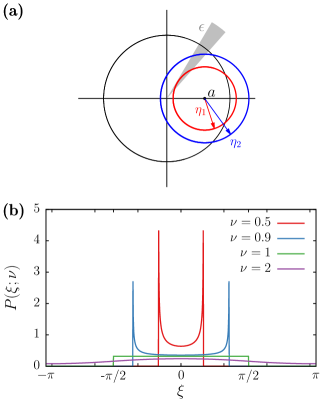
Figure 1: (a) Geometric interpretation of the noise effects in the vectorial Vicsek model. The red and blue circles depict the circle $re^{i\xi}=a+\eta e^{i\chi}$ corresponding to two $\eta_{1}=0.5$ (red) and $\eta_{2}=0.7$ (blue), both cases with a local polarization of $a=0.6$. The grey shaded area indicates an interval $\epsilon$ over which the arclength needs to be computed to obtain $P(\xi)$. (b) Shape of $P(\xi;\nu)$ for different values of $\nu=\eta/a$, as obtained by Eq. (17).

Fig. 1(b) shows the shape of $P(\xi;\nu)$ for various values of $\nu$. The piecewise character of $P$ illustrates the strong effects of the vectorial noise. If the local polarization of the particle $a$ is smaller than the noise strength $\eta$ (i.e., $\nu>1$), then the distribution is unimodal, with $\xi$ ranging within $(-\pi,\pi)$, and tends to the uniform distribution $P(\xi)=1/2\pi$ in the limit $\nu\to\infty$. On the other hand, if the local polarization is larger than the noise strength (i.e., $\nu<1$), then the probability density is concentrated at the extreme values of the distribution $\pm\arcsin\left(\frac{\eta}{a}\right)$. In the limit of $\nu\to 0$, the extremes of the distribution coalesce to yield a delta function, as can be checked in Fourier space.

III Multiplicative models for the angular noise distribution

The form of multiplicative noise distribution shown by the Vicsek model with angular distribution of amplitude (variance) depending on $\nu=\eta/a$, represents a physically motivated choice, in which the fluctuations of the particle orientation around the direction of the local polarization, $\Theta_{i}(t)$, are an increasing function of the noise strength $\eta$ and a decreasing function of the local polarization $a_{i}$, meaning that an individual has a stronger tendency to follow the average direction of a group if this group is very coherent (an explicit mathematical relation is derived in Section IV). For this reason, in the following we will consider two additional models characterized by an angular distribution with a multiplicative nature: a simple wrapped Gaussian noise, and a more physically motivated bivariate Gaussian distribution.

III.1 Wrapped Gaussian noise

Gaussian distributions represent a natural choice for typical distributions of noise in mathematical models. In the present case, the noise term has a distribution with support in the unit circle. Therefore, the natural extension of Gaussian noise is provided by a Gaussian distribution defined at the scalar level and then projected on the unit circle. We thus consider a model in with the angular noise distribution $P(\xi;a,\eta)$ is a normal distribution with standard deviation $\sigma=\eta/a$ wrapped on the circle. The resulting probability density reads Mardia and Jupp (2009),

$$P(\xi;a,\eta)=\frac{a}{\eta\sqrt{2\pi}}\sum_{m=-\infty}^{\infty}\exp\left[\frac{-a^{2}(\xi+2\pi m)^{2}}{2\eta^{2}}\right]\;.$$ (18)

Practically, one just simulates a usual Gaussian variable $\zeta$ and then wraps it to $[0,2\pi)$ as $\xi=\zeta\;\;(\text{mod }2\pi)$.

III.2 Bivariate Gaussian noise

The inclusion of vectorial noise in the Vicsek model is meant to account, in average, for the inaccuracy of the single individuals in determining the exact direction of their neighbors Grégoire and Chaté (2004); Chaté et al. (2008). Here we propose a different noise term also aimed to capture these errors. The main idea consists of adding a bivariate Gaussian random variable for each particle in the computation of the mean direction, that can be interpreted as making a small error in the determination of the orientation of each neighbor. Formally, this model can be formulated as

$$\theta_{j}(t+1)=\arg\left\{\frac{1}{|\mathcal{N}_{j}|}\sum_{k\in\mathcal{N}_{j}}\left(e^{i\theta_{k}(t)}+\boldsymbol{\zeta}_{j}^{(k)}(t)\right)\right\},$$ (19)

where the real and imaginary parts of the complex numbers $\boldsymbol{\zeta}^{(k)}_{j}=\alpha^{(k)}_{j}+i\beta_{j}^{(k)}$ are independent Gaussian variables with zero mean and variance $\sigma^{2}$. This equals to consider that the vectors $(\alpha_{j}^{(k)},\beta_{j}^{(k)})$ are bivariate Gaussian variables with covariance matrix $\sigma^{2}\boldsymbol{I}$. Then one can sum the contributions of the different Gaussian terms so that the system reads

$$\theta_{j}(t+1)=\arg\left\{a_{j}e^{i\Theta_{j}}+\frac{1}{\sqrt{|\mathcal{N}_{j}|}}\boldsymbol{\zeta}_{j}(t)\right\}\;,$$ (20)

where $\boldsymbol{\zeta}_{j}=\alpha_{j}+i\beta_{j}$ and $(\alpha_{j},\beta_{j})$ are also bivariate Gaussian variables with covariance $\sigma^{2}\boldsymbol{I}$. The argument of a bivariate Gaussian random variable centered at $(a_{j}\cos(\Theta_{j}),a_{j}\sin(\Theta_{j}))$ and standard deviation $\sigma$ follows a projected normal distribution Mardia and Jupp (2009). Since the projected normal distribution is closed under rotations, the generalized Vicsek model with bivariate Gaussian noise can be written in the form

$$\theta_{j}(t+1)=\arg\left\{a_{j}e^{i\Theta_{j}}\right\}+\xi_{j}(t),$$ (21)

where $\xi_{j}$ is a projected normal angular variable centered at $(a_{j},0)$ and covariance matrix $\sigma^{2}\boldsymbol{I}/\sqrt{|\mathcal{N}_{j}|}$. Notice that the mean direction $\Theta_{j}$ does not have an impact on the noise distribution, whereas the local polarization $a_{j}$ does.

In this particular case there are two sources of multiplicative effects: The local polarization $a_{j}$ and the number of neighboring particles $|\mathcal{N}_{j}|$. The study of the impact of the number of neighboring particles on the system is beyond the scope of this paper and we leave it for future studies. Instead, we consider a simplified version where the standard deviation of the variables $\alpha_{j}$ and $\beta_{j}$ is just the control parameter $\eta$. Accordingly, the probability density for the random variables $\xi$ as formulated in Eq. (5) is a projected normal distribution corresponding to a bivariate Gaussian centered at $a$ and with standard deviation $\eta$, which leads to (see Eq.(3.5.48) in Ref. Mardia and Jupp (2009))

$$P(\xi;a,\eta)=c_{0}+\frac{a}{\eta}\cos(\xi)\Phi\left(\frac{a}{\eta}\cos(\xi)\right)f\left(\frac{a}{\eta}\sin(\xi)\right)$$ (22)

where $c_{0}=\exp{\left(\frac{-a^{2}}{2\eta^{2}}\right)}/(2\pi)$ is a constant and $\Phi(z)$ and $f(z)$ are the cumulative distribution and probability density functions of a normally distributed random variable with zero mean and unit variance, respectively. It is worth noticing that, again, the distribution only depends on the parameter, $\eta/a$, which arises naturally by implementing the projection of the stochastic vectors on the unit circle.

IV Mean-field theory

We can gain a preliminar understanding of the properties of our class of models by means of a mean-field analysis, by which we mean the limit case in which each SPP interacts with all other particles or, in other words, when interactions are mediated by a fully connected network. In this case, we have

$$\Phi=\phi e^{i\alpha}=\frac{1}{N}\sum_{j=1}^{N}e^{i\theta_{j}}$$ (23)

where $\phi=|\Phi|$ denotes the order parameter of the system. The velocity of each variable is updated according to

$$\theta_{j}(t+1)=\alpha(t)+\xi_{j}(t)\;,$$ (24)

thus, one can write an equation for the evolution of the order parameter as

$$\phi(t+1)=\frac{1}{N}\left|\sum_{j=1}^{N}e^{i\alpha(t)+i\xi_{j}(t)}\right|=\frac{1}{N}\left|\sum_{j=1}^{N}e^{i\xi_{j}(t)}\right|\;.$$ (25)

The distribution of each $\xi_{j}$ depends, in principle, on $\eta$ and the local polarization $a_{j}$. In the mean-field level, however, $a_{j}=\phi$. The subindices on the previous equation can thus be dropped to obtain

$$\phi(t+1)=\frac{1}{N}\left|\sum_{j=1}^{N}e^{i\xi_{j}(t)}\right|\;.$$ (26)

Invoking the thermodynamic limit ($N\to\infty$) one finally obtains the evolution equation of the mean-field as

$$\phi(t+1) = E[\cos(\xi)]=\int_{-\pi}^{\pi}P(\xi;\phi(t),\eta)\cos(\xi)d\xi$$ (27)

$$\equiv \rho(\phi(t),\eta)\;,$$ (28)

where we are using the fact that the distribution $P$ is symmetric and centered at zero. The fixed points of the previous equation correspond to the stationary states of the mean-field solution, which are obtained as the solution of the self-consistent mean-field equation

$$\phi=\rho(\phi,\eta)=\int_{-\pi}^{\pi}P(\xi;\phi,\eta)\cos(\xi)d\xi.$$ (29)

In circular statistics the quantity $\rho=E[\cos(\xi)]$ is known as mean resultant length and it is a well studied measure of concentration Mardia and Jupp (2009). Moreover, the circular variance of an angular distribution is usually defined as $V=1-\rho$. The fact that, in a globally coupled system, the order parameter of the system corresponds exactly to the mean resultant length of the noise distribution $P(\xi)$ is an important result that simplifies the analysis of the mean-field dynamics.

In the following, we will consider the mean-field solution of the models defined by the angular distributions considered above.

IV.1 Scalar Vicsek model

The original Vicsek model, characterized by the probability distribution presented in Eq. (8), presents the mean-field solution

$$\phi(\eta)=\rho(\eta)=\frac{\sin(\pi\eta)}{\pi\eta}\;,$$ (30)

which does not undergo any phase transition except at the limiting value $\eta=1$, for which the system becomes disordered Miguel, Parley, and Pastor-Satorras (2018). In Fig. 2(a) we present a plot of the shape of the mean-field order parameter as a function of $\eta$.

IV.2 Vectorial Vicsek model

The vectorial Vicsek model, defined by the angular noise distribution Eq. (17), has a mean resultant length for $\nu>1$, of the form

$$\rho=\int_{-\pi}^{\pi}d\xi\frac{\cos^{2}\xi}{2\pi\sqrt{\nu^{2}-\sin^{2}\xi}}=\frac{1}{2\nu}{{}_{2}F_{1}}\left(\frac{1}{2},\frac{1}{2};2,\frac{1}{\nu^{2}}\right),$$ (31)

where ${{}_{2}F_{1}}$ is the hypergeometric function Abramowitz and Stegun (1965). For the case $\nu\leq 1$, denoting $\xi_{0}=\arcsin(\nu)$, we obtain

$$\rho=\int_{-\xi_{0}}^{\xi_{0}}d\xi\frac{\cos^{2}\xi}{\pi\sqrt{\nu^{2}-\sin^{2}\xi}}={{}_{2}F_{1}}\left(\frac{1}{2},\frac{-1}{2};1,\nu^{2}\right)\;.$$ (32)

Using the fact that $\nu=\eta/\phi$ we obtain the mean-field equation for the Vicsek model with vectorial noise,

$$\phi=\rho(\phi,\eta)=\begin{cases}\displaystyle{\frac{\phi}{2\eta}{{}_{2}F_{1}}\left(\frac{1}{2},\frac{1}{2};2,\frac{\phi^{2}}{\eta^{2}}\right)}&\phi<\eta\\[10.0pt] \displaystyle{{{}_{2}F_{1}}\left(\frac{1}{2},\frac{-1}{2};1,\frac{\eta^{2}}{\phi^{2}}\right)}&\phi\geq\eta\end{cases}$$ (33)

We notice that this result was already reported in Pimentel et al. (2008), obtained using a completely different approach. An explicit solution for $\phi=\rho(\phi,\eta)$ is, as far as we know, out of reach. However, in the present case of multiplicative noise, since the angular noise distribution depends on the ratio $\nu=\eta/\phi$, we can write the mean-field equation as

$$\eta=\frac{\eta}{\phi}\rho\left(\frac{\eta}{\phi}\right)\equiv\nu\rho(\nu).$$ (34)

As a result, the mean-field solution can be obtained numerically simply by plotting the noise parameter $\eta(\nu)=\nu\rho(\nu)$, as a function of $\nu$, and obtaining the order parameter from the expression $\phi=\eta(\nu)/\nu$. The red curve in Fig. 2(b) shows the monotonically increasing relation between the circular variance, $V=1-\rho$, and the distribution parameter $\nu$, whereas the inset shows the form of $\eta(\nu)$ as a function of $\nu$. In Fig. 2(a) we plot the corresponding mean-field solution. The continuous line indicates a stable fixed point, whereas the dashed line indicates unstable solutions. The curves are accompanied by results of numerical simulations of the mean-field system for $N=10^{4}$ starting from an ordered state.

While the original Vicsek model does not present a phase transition in the mean-field limit, the vectorial Vicsek model does display one: for large $\eta$ only the disordered solution exists (i.e., $\phi=0$). As noise is reduced, two new solutions appear through a saddle-node bifurcation at $\eta_{c}\simeq 0.6715$ (determined numerically), thus corresponding to a discontinuous phase transition. Only one of the two new solutions is stable. For a range of intermediate values of $\eta$ there is multistability between the ordered and disordered states. The value $\eta_{c^{\prime}}$ for which the solution $\phi=0$ collides with the unstable state and loses stability can be obtained analytically as

$$\frac{d}{d\phi}\rho(\phi,\eta_{c^{\prime}})\biggr{|}_{\phi=0}=\frac{1}{2\eta_{c^{\prime}}}{{}_{2}F_{1}}\left(\frac{1}{2},\frac{1}{2};2,0\right)=\frac{1}{2\eta_{c^{\prime}}}=1\;.$$ (35)

Hence for $\eta<\eta_{c^{\prime}}=1/2$ only the ordered state is stable.

IV.3 Wrapped Gaussian noise

For the wrapped Gaussian noise, defined by the angular noise distribution in Eq. (18), the mean resultant length takes the form (see Eq.(3.5.63) from Ref. Mardia and Jupp (2009))

$$\rho=\exp\left(-\frac{\eta^{2}}{2\phi^{2}}\right),$$ (36)

which, from the mean-field equation $\phi=\rho(\phi,\eta)$, leads to the implicit mean-field solution

$$\eta=\phi\sqrt{-2\log(\phi)}\;,$$ (37)

which is valid only for $\phi>0$. However, since, for finite $\eta>0$,

$$\lim_{\phi\to 0}\rho(\phi,\eta)=0\;,$$ (38)

we can see that the solution $\phi=0$ exists as a limiting case.

The wrapped Gaussian distribution exhibits a discontinuous phase transition at the mean-field level. The equation Eq. (36) has two branches of solutions, a stable and an unstable one. Both branches coexist with the disordered state $\phi=0$, which is stable for all values of $\eta$. The ordered state vanishes at the local maximum of $\eta$ in Eq. (37), which yields a transition point $\eta_{c}=e^{-1/2}$ with the jump of the discontinuous transition being also $\phi_{c}=e^{-1/2}$. In Fig. 2(a) we present a plot of the resulting mean-field solution for the order parameter $\phi$. Also in this case, the (circular) variance of the distribution increases with $\nu$, as illustrated by the green line in Fig. 2(b).

IV.4 Bivariate Gaussian distribution

The bivariate Gaussian distribution, characterized by the angular noise distribution Eq. (22), has an associated mean resultant length Kendall (1974),

$$\rho=\frac{\phi}{2\eta}\sqrt{\frac{\pi}{2}}e^{-\frac{\phi^{2}}{4\eta^{2}}}\left[I_{0}\left(\frac{\phi^{2}}{4\eta^{2}}\right)+I_{1}\left(\frac{\phi^{2}}{4\eta^{2}}\right)\right]\;$$ (39)

where $I_{0}(z)$ and $I_{1}(z)$ are modified Bessel functions of the first kind Abramowitz and Stegun (1965).

In this case, the mean-field equation $\phi=\rho(\phi,\eta)$ leads to a continuous phase transition, as a numerical analysis based on Eq. (34) shows. As indicated by the blue squares in Fig 2(a), upon reducing $\eta$ the disordered state ($\phi=0$) loses stability through a pitchfork bifurcation, giving raise only to one new meaningful stable state. Although the mean-field equation is hard to analyze, it is possible to compute the critical point value $\eta_{c}$, since it corresponds to the loss of stability of the disordered solution $\phi=0$. Hence, $\eta_{c}$ is given by

$$\frac{d}{d\phi}\rho(\phi,\eta)\biggr{|}_{\phi=0}=\frac{1}{2\eta_{c}}\sqrt{\frac{\pi}{2}}=1$$ (40)

thus $\eta_{c}=\frac{1}{2}\sqrt{\frac{\pi}{2}}\simeq 0.627$. Using this value it is possible to compute the critical exponent $\beta$ for the phase transition. Performing a Taylor expansion on both sides of the mean-field equation $\phi=\rho(\phi,\eta)$ for $\phi\ll 1$ up to third order one obtains the relation

$$1=\frac{\eta_{c}}{\eta}\left(1-\frac{\phi^{2}}{8\eta^{2}}\right)\;.$$ (41)

Solving for $\phi$ and taking $\eta\to\eta_{c}$ finally leads to

$$\phi=\frac{2\sqrt{2}\eta}{\sqrt{\eta_{c}}}\left(\eta_{c}-\eta\right)^{\frac{1}{2}}\propto(\eta_{c}-\eta)^{\frac{1}{2}}\;,$$ (42)

thus near the transition the order parameter scales with an exponent of $\beta=1/2$.

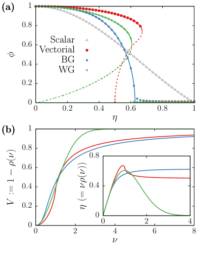
Figure 2: (a) Mean-field transitions for the four different types of noise, namely original scalar noise (grey triangles), vectorial noise (red circles), bivariate Gaussian (blue squares), and wrapped Gaussian (green plusses). Symbols correspond to simulations with $N=10^{4}$ particles starting from a fully ordered state. Lines have been obtained from the analytical results. A continuous line indicates a stable solution, whereas dashed lines correspond to unstable fixed points. (b) Dependence of the circular variance, defined as $V=1-\rho$, on the parameter $\nu=\eta/\phi$ for the three multiplicative distributions (same colors as in (a)). Inset shows the dependence of the control parameter on the distribution parameter $\nu$.

IV.5 Nature of the transition in multiplicative noise models

Surprisingly, despite being qualitatively quite similar, the three distributions with multiplicative noise exhibit an order-disorder transition with three different scenarios. The Vicsek model with vectorial noise has a first order bifurcation with a small region of bistability; the wrapped Gaussian noise model shows a first order bifurcation coexisting with a disordered state for all values of $\eta$; and the bivariate Gaussian noise model presents a continuous, second order phase transition. Such differences are not obvious from the definition of each distribution. In fact, in all three cases the amplitude (variance) of the distribution increases with $\nu$, being more prominent for the Wrapped Gaussian noise (see Fig 2(b)).

In order to understand a priori which choices of the angular noise distribution lead to each of these different cases, one should notice that, from the mean-field equation, $\rho(\nu)=\phi$. Hence, at the fixed points different from the disordered state $\phi=0$, the distribution parameter $\nu=\eta/\phi$ can be written as $\nu=\eta/\rho(\nu)$. Therefore, the mean-field solutions corresponding to the ordered phase appear as the values of the control parameter as a function of $\nu$, $\eta=\nu\rho(\nu)$ (see Eq. (34)). The inset of Fig. 2(b) presents the functions $\nu\rho(\nu)$ for all the cases studied here. These functions show whether for a fixed $\eta$ there are one or two additional solutions to the disordered case. The existence of a local maximum indicates the presence of two ordered solutions in the vicinity of the maximum, and thus the presence of a first-order transition, whereas a monotonic function characterizes a second-order transition.

The two discontinuous first-order transitions presented here emerge as a saddle-node bifurcation of a system at the thermodynamic limit. Moreover, the order parameter behaves as

$$\phi-\phi_{c}\propto(\eta_{c}-\eta)^{\beta}$$ (43)

where $\phi_{c}$ is the height of the jump at the discontinuity and $\beta$ is a characteristic exponent. According to this observation, we are therefore in front of a hybrid phase transition Dorogovtsev, Goltsev, and Mendes (2006); Goltsev, Dorogovtsev, and Mendes (2006), that is, a phase transition that exhibits a jump in the order parameter, as in first order transitions, accompanied by a critical singularity, as in second order transitions. For the Vicsek model with vectorial noise we estimate the value of the critical exponent numerically as $\beta\simeq 0.5$ (see Table 1). For the wrapped Gaussian noise, recalling that $\phi_{c}=\eta_{c}=e^{-1/2}$, the critical exponent can be obtained as

$$\beta=\lim_{\phi\to\phi_{c}}\frac{\log\left(\phi-\phi_{c}\right)}{\log\left(\eta_{c}-\phi\sqrt{-2\log\phi}\right)}=\frac{1}{2}.$$ (44)

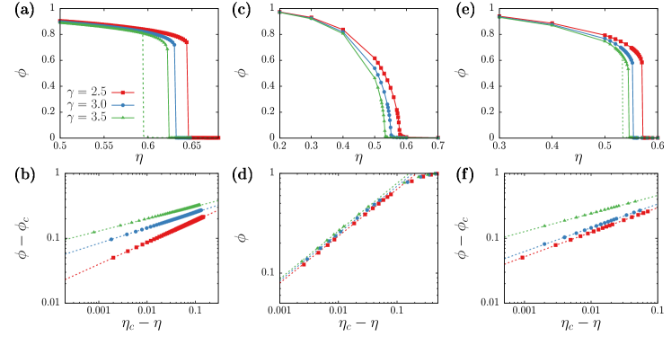
Figure 3: Results of the generalized Vicsek models with fixed interactions given by power-law distributed networks with $N=10^{6}$ nodes and degree distribution exponent $\gamma=2.5$ (red squares), 3 (blue circles), and 3.5 (green triangles). Top panels show the behavior of the order parameter $\phi$ for different values of $\eta$, whereas bottom panels show the corresponding scaling behavior close to the transition, with dashed lines indicating the results of a nonlinear fitting. (a,b) Vectorial model. (b,c) Bivariate Gaussian noise. (c,d) Wrapped Gaussian noise. Dashed green lines in panels (a) and (c) display the results obtained by initializing the system at random for the case $\gamma=3.5$. All other results have been obtained starting from a fully ordered initial condition, with all SPPs pointing in the same direction. Simulations computed over a total of $2.5\cdot 10^{5}$ time steps, with a thermalization of $5\cdot 10^{4}$ time steps.

V Multiplicative noise models on networks

In order to gain some understanding of the applications of mean-field theory in our class of flocking dynamics models, we consider the case in which interactions are mediated by a static complex network Newman (2010). The relevance of this case is based on the recent claims that a network structure, representing the patterns of social interactions Croft, James, and Krause (2008), can be relevant in understanding the flocking behavior of social animals Bode, Wood, and Franks (2011a, b); Miguel, Parley, and Pastor-Satorras (2018); Miguel and Pastor-Satorras (2019); Ling et al. (2019), which might have a stronger tendency to follow individuals with which they have stronger social ties Ling et al. (2019). Previous works have shown that the scalar Vicsek model with networked interactions display a second-order transition Pimentel et al. (2008); Miguel, Parley, and Pastor-Satorras (2018), whose properties depend on the degree of heterogeneity of the network. Here we present the results of numerical simulations of generalized Vicsek models with multiplicative noise on uncorrelated networks with a heterogeneous degree distribution given by a power law $P(k)\sim k^{-\gamma}$, generated with the uncorrelated configuration model (UCM) Catanzaro, Boguñá, and Pastor-Satorras (2005). We consider networks of size $N=10^{6}$ and different degree exponents $\gamma=2.5$, $3.0$, and $3.5$. Our results are presented in Fig. 3, where we display the time averaged order parameter $\phi$ computed over a time span of $2\cdot 10^{5}$ time steps after a thermalization of $5\cdot 10^{4}$ time steps. Results are computed starting from a completely ordered state, except for the dashed green lines in Figures 3(a,c), where the SPPs initially point to randomly chosen directions.

In the case of the vectorial Vicsek model, see Fig. 3(a), we are clearly in presence of a first-order transition. The critical value $\eta_{c}$, at which the discontinuity of the order parameter takes place, decreases with the degree exponent $\gamma$, but the overall discontinuous character of the transition seems to be preserved. The hybrid nature of the transition, predicted by the mean-field analysis, is still manifest on networks, given by a critical singularity in the vicinity of the transition in the ordered phase described by Eq. (43). Fig. 3(b) shows this behavior, with the dashed lines being the result of a non-linear fitting procedure. A decrease of $\beta$ upon increasing $\gamma$ can be appreciated. Table 1 reports the estimated values of $\beta$ for each case, as obtained from the non-linear fitting.

For the case of the model with bivariate noise, the transition displayed in networks has a second-order nature, again in agreement with mean-field theory, see Fig. 3(c). The critical exponent $\beta$ characterizing the transition appears to have a value roughly independent of the critical exponent, and just slightly below the mean-field value $\beta=1/2$, see Table 1 and Fig. 3(d)).

The wrapped Gaussian case follows the same trend than the previous instances: The behavior of the order parameter follows that of the mean-field (see Fig. 3(e)), including the hybrid behavior close to the discontinuity. In this case the numerically estimated values of $\beta$ also change with $\gamma$ as in the vectorial model, see Table 1 and Fig. 3(f).

Finally, in order to illustrate the existence of multistability in the vectorial and wrapped Gaussian noise, the green dashed lines in Figs. 3(a,c) show the order parameter obtained in simulations starting from random initial conditions, in which the SPPs point to randomly chosen directions. Only results for $\gamma=3.5$ are shown, although the multistability of the vectorial and wrapped Gaussian noise is present for all the tested networks.

Table 1: Estimated values of $\beta$ in mean-field and in power-law distributed networks with degree exponent $\gamma$. The mean-field values for the wrapped Gaussian and the bivariate Gaussian are analytical results. The mean-field value for the vectorial has been obtained through a linear fitting of the log-log data. The values for the networks have been obtained through a non-linear fitting algorithm.

	Mean-field	$\gamma=2.5$	$\gamma=3.0$	$\gamma=3.5$
Vectorial	$0.489(3)$	$0.34(2)$	$0.24(2)$	$0.19(5)$
Bivariate Gaussian	1/2	$0.47(1)$	$0.48(2)$	$0.48(1)$
Wrapped Gaussian	1/2	$0.38(3)$	$0.37(2)$	$0.28(2)$

VI Multiplicative noise models on Euclidean space

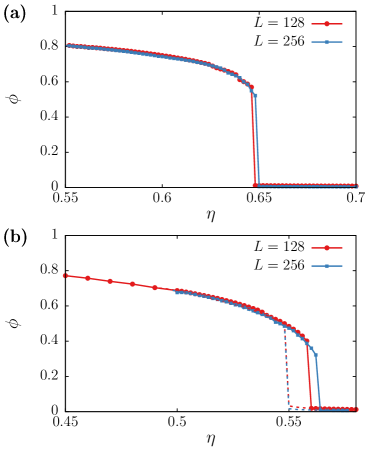
Figure 4: Sample order parameter $\phi$ obtained from numerical simulations in 2D space with metric interactions. (a) Results of the vectorial Vicsek model. (b) Results of the Vicsek model with wrapped Gaussian noise. Results correspond to systems with density $n=2$ and size $L=128$ (red circles) and $256$ (blue squares). The length of the simulations is $2.5\cdot 10^{5}$ time steps including a thermalization of $5\cdot 10^{4}$ time steps. Each simulation initial condition corresponds to the final configuration of the previous simulation. Continuous lines and points correspond to $\eta$ being increased, whereas dashed lines in panel (b) correspond to decreasing $\eta$.

We finally study the effect of different multiplicative noise terms in a two dimensional space in which the interactions between SPPs are determined by the position of each unit. The spatial short-range interactions correspond to the formulation of the original scalar Vicsek Vicsek et al. (1995), in which interacting neighbors are chosen following the metric rule in Eq. (6). Nowadays it is well known that both the original and vectorial formulations of the Vicsek model with short-range spatial interactions display a first-order transition with a coexistence region. Whereas for the vectorial model this situation is readily seen and in agreement with the mean-field results, the first-order character of the original Vicsek model has been largely debated, since the transition appears to be affected by strong finite-size effects Aldana, Larralde, and Vázquez (2009); Chaté, Ginelli, and Grégoire (2007); Ginelli (2016); Chaté et al. (2008); Aldana, Larralde, and Vázquez (2009). Nonetheless, the evidence clearly indicates that, with periodic boundary conditions, the transition from disorder to order remains discontinuous, with a region of coexistence characterized by the formation of bands of high density in the ordered phase Grégoire and Chaté (2004); Ginelli (2016); Chaté et al. (2008); Chaté (2020). The fact that the Vicsek model in the space presents a transition much different from that seen in complex networks or the mean-field limit is due to the strong effects caused by the interplay between density and coupling arising from the short-range spatial interactions. Changing the way in which such short-range interactions are established can lead to qualitative different behavior. This is the case, for instance, of non-metric interactions Ginelli and Chaté (2010). Therefore, it is a priori unclear which behavior we are going to observe in the different models of multiplicative noise we consider here.

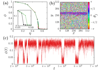
Figure 5: (a) Order parameter $\phi$ obtained as a time average from numerical simulations of the model with spatial interactions and bivariate Gaussian noise. Red squares, blue circles, and green triangles correspond to simulations with a lattice of side length $L=128$, 256, and 512, with density $n=2$. The inset shows the hysteresis loop obtained by adiabatically increasing (green triangles) and decreasing (black stars) $\eta$. Each simulation has been computed over a time window of $2.5\cdot 10^{5}$ time steps including a thermalization of $5\cdot 10^{4}$ time steps. (b) Snapshot of the system at the ordered state for $L=512$, $n=2$, and $\eta=0.525$. The color of each particle indicates the orientation. Only $10\%$ of the particles are shown. (c) Time series of the order parameter for $L=256$ and $\eta=0.521$ showing bistability between the ordered and disordered phases in a longer simulation.

In Fig. 4 we display the results of numerical simulations for vectorial and wrapped Gaussian models with metric interactions on a square of size $L$ endowed with periodic boundary conditions. In our simulations the system size scales with $L$ so that the density of particles is kept constant to the value $n=N/L^{2}=2$. We used a radius of interaction with neighboring particles of $r_{0}=1$ and the particles move at a speed $v_{0}=0.5$. The length of the simulations is $2.5\cdot 10^{5}$ time steps, including a thermalization of $5\cdot 10^{4}$ time steps. Simulations have been performed adiabatically increasing $\eta$, except for dashed lines of Fig. 4(b), which correspond to an adiabatic decrease of the control parameter $\eta$. Both vectorial and wrapped Gaussian distribution noise models display a clear discontinuous transition, with a region of coexistence of ordered bands and disorder. Beyond the coexistence region the bands become unstable and the Toner-Tu ordered phase predominates. Overall, the scenario is consistent with the usual bifurcation diagram of the scalar Vicsek model Chaté (2020). In this case, the existence of an hybrid scaling behavior at the transition point is not clear, as simulations of the spatial systems display strong finite size effects.

More interesting is the case of the bivariate Gaussian noise. Fig. 5(a) shows the results obtained for different system sizes. Although the transition appears to be continuous for small systems, for large enough sizes ($L=256$ and $512$) it is possible to observe a discontinuity on $\phi$, including an hysteresis loop (see inset of Fig. 5(a)). Moreover, as reported in Fig. 5(b), snapshots of the simulations close to the transition point show the existence of bands of ordered particles, a signature of the classical bifurcation diagram of self-propelled polar particles Chaté (2020). Finally, Fig. 5(c) shows a time series of the order parameter for $L=256$, where the bistability between the ordered and disordered phases becomes evident. Therefore, despite finite-size effects, our results indicate that all spatial models share a universal first-order transition towards the formation of ordered bands, with a coexistence region.

VII Discussion

Simple models of SPPs provide a framework to study the mechanisms underlying the onset of self-organized collective motion. In this paper we introduced and studied a class of Vicsek-like models where the system dynamics depends on two key elements: the definition of neighboring particles towards which an individual tends to align, and a stochastic source of angular noise that models the difficulties of a single individual to perfectly align with its neighbors. Previous studies considered different instances of interaction rulesGinelli and Chaté (2010); Bode, Wood, and Franks (2011a); Miguel, Parley, and Pastor-Satorras (2018), but less work has been devoted to the effect of different sources of angular noise on the onset of collective motion. Two main stochastic angular noise terms have been used in the literature: The uniform distribution introduced on the original Vicsek model, and the vectorial noise proposed by Grégoire and H. Chaté Grégoire and Chaté (2004), which, as we show, induces a multiplicative effect. Our derivation of the angular probability distribution for the vectorial noise provides an explicit relation between the local polarization of a SPP and the noise intensity, which appears to be mediated by the parameter $\nu=\eta/a$. Remarkably, the resulting probability density turns out to be rather non-generic, with a piecewise distribution that is peaked at the extremes for small noise values (or large local polarization), and unimodal otherwise.

We have extended the analysis of multiplicative noise in Vicsek-like models by proposing two simpler and more generic angular probability distributions for the stochastic source. The case of bivariate Gaussian noise is conceptually similar to that of the vectorial noise, where the angular distribution needs to be computed a posteriori. In this case, the parameter $\nu=\eta/a$ also arises naturally from the definition of the system. On the other hand, the multiplicative character of the wrapped Gaussian distribution is imposed with the definition of a standard deviation that depends on the local polarization.

Despite being qualitatively similar, the differences between the three multiplicative models studied here arises already at the mean-field level, which is given in a generic form by solving a self-consistent equation involving the mean-resultant length of the angular distribution. Surprisingly, the character of the transition changes greatly with the choice of the stochastic term, being a first-order hybrid transition for the vectorial and wrapped Gaussian distribution, and second order for the bivariate Gaussian model. Simulations in complex networks show a scenario consistent with that of the mean-field analysis, where different choices for the noise leads to different behavior.

On the other hand, the emergence of collective motion in spatial models with short-range interactions follows a mechanism of a different nature. In all the studied cases, numerical simulations with large enough number of particles reveal a first-order transition including hysteresis and the formation of high-density bands. The scenario is reminiscent of that of the original Vicsek model, where the phase transition for the spatial model does not correspond to that seen in the mean-field or networked models Chaté (2020); Chaté, Ginelli, and Grégoire (2007). Therefore we conclude that the interplay between density and coupling that acts on spatial models induces a rather generic phase diagram in which the peculiarities of the noise distributions considered here play a minor role.

A single SPPs on a Vicsek-like model can be interpreted as an interacting random walker in a two dimensional space. Accordingly, the inclusion of multiplicative noise in the model induces a correlation between the direction of the next step and the state of the system. This idea brings the multiplicative models studied here close to the model of active matter through persistent random walkers proposed by Escaff et al. Escaff et al. (2018) in one dimension. In their model an individual changes its direction only at certain time steps with a frequency that depends on the local polarization. In our case a change in direction happens at all times, but it is much smaller if the local polarization is high. Thus we believe that a two dimensional model based on the idea of persistent random walks should produce similar behavior than the one exposed here, as well as could benefit from the analytical tools existing for that case.

The study of minimal models provides solid grounds to study complex phenomena and understand the effects of the different elements that compose the model on the overall onset of collective motion. On the other hand, it is also important to work on realistic setups in order to retain new sources for other types of phenomenology. To this extend, possible extensions of our work include considering continuous time models and allowing for steps of different length (variable velocity) Farrell et al. (2012), which can be correlated with the local polarization and/or the random turning angle. Finally, in line with the growing experimental work on the field Aoki (1982); Narayan, Ramaswamy, and Menon (2007); Sanchez et al. (2012); DeCamp et al. (2015); Li et al. (2018), future work should also study the validity of the different models on the basis of empirical evidence.

Data availability

The network topologies used in the numerical simulations that support the findings of this study are available from the corresponding author upon request.

References

- Couzin and Krause (2003) I. D. Couzin and J. Krause, “Self-Organization and Collective Behavior in Vertebrates,” in Advances in the Study of Behavior (2003) pp. 1–75.
- Sumpter (2006) D. J. T. Sumpter, “The principles of collective animal behaviour,” Philosophical Transactions of the Royal Society B: Biological Sciences 361, 5–22 (2006).
- Sumpter (2010) D. J. Sumpter, Collective Animal Behavior (Princeton University Press, New Jersey, 2010).
- Giardina (2008) I. Giardina, “Collective behavior in animal groups: Theoretical models and empirical studies,” HFSP Journal 2, 205–219 (2008).
- Vicsek and Zafeiris (2012) T. Vicsek and A. Zafeiris, “Collective motion,” Phys. Rep. 517, 71–140 (2012).
- Lopez et al. (2012) U. Lopez, J. Gautrais, I. D. Couzin, and G. Theraulaz, “From behavioural analyses to models of collective motion in fish schools,” Interface Focus 2, 693–707 (2012).
- Aoki (1982) I. Aoki, “A simulation study on the schooling mechanism in fish,” Nippon Suisan Gakkaishi 48, 1081–1088 (1982).
- Reynolds (1987) C. W. Reynolds, “Flocks, herds and schools: A distributed behavioral model,” SIGGRAPH Comput. Graph. 21, 25–34 (1987).
- Goldenfeld (1992) N. Goldenfeld, Lectures On Phase Transitions And The Renormalization Group (CRC Press, Boca Raton FL, 1992).
- Vicsek et al. (1995) T. Vicsek, A. Czirók, E. Ben-Jacob, I. Cohen, and O. Shochet, “Novel type of phase transition in a system of self-driven particles,” Phys. Rev. Lett. 75, 1226–1229 (1995).
- Ginelli (2016) F. Ginelli, “The physics of the vicsek model,” The European Physical Journal Special Topics 225, 2099–2117 (2016).
- Yeomans (1992) J. M. Yeomans, Statistical mechanics of phase transitions (Oxford University Press, Oxford, 1992).
- Grégoire and Chaté (2004) G. Grégoire and H. Chaté, “Onset of collective and cohesive motion,” Phys. Rev. Lett. 92, 025702 (2004).
- Ginelli and Chaté (2010) F. Ginelli and H. Chaté, “Relevance of metric-free interactions in flocking phenomena,” Phys. Rev. Lett. 105, 168103 (2010).
- Bode, Wood, and Franks (2011a) N. W. Bode, a. J. Wood, and D. W. Franks, “The impact of social networks on animal collective motion,” Animal Behaviour 82, 29–38 (2011a).
- Miguel, Parley, and Pastor-Satorras (2018) M. C. Miguel, J. T. Parley, and R. Pastor-Satorras, “Effects of heterogeneous social interactions on flocking dynamics,” Phys. Rev. Lett. 120, 068303 (2018).
- Gao et al. (2011) J. Gao, S. Havlin, X. Xu, and H. E. Stanley, “Angle restriction enhances synchronization of self-propelled objects,” Phys. Rev. E 84, 046115 (2011).
- Ngo, Ginelli, and Chaté (2012) S. Ngo, F. Ginelli, and H. Chaté, “Competing ferromagnetic and nematic alignment in self-propelled polar particles,” Phys. Rev. E 86, 050101 (2012).
- Dorogovtsev, Goltsev, and Mendes (2006) S. N. Dorogovtsev, A. V. Goltsev, and J. F. F. Mendes, “k-core organization of complex networks,” Physical Review Letters 96, 040601 (2006).
- Goltsev, Dorogovtsev, and Mendes (2006) A. V. Goltsev, S. N. Dorogovtsev, and J. F. F. Mendes, “k-core (bootstrap) percolation on complex networks: Critical phenomena and nonlocal effects,” Physical Review E 73, 056101 (2006), 0602611 [cond-mat] .
- Newman (2010) M. Newman, Networks: An Introduction (Oxford University Press, Inc., New York, NY, USA, 2010).
- Chaté (2020) H. Chaté, “Dry Aligning Dilute Active Matter,” Annual Review of Condensed Matter Physics 11, 189–212 (2020).
- Mardia and Jupp (2009) K. Mardia and P. Jupp, Directional Statistics, Wiley Series in Probability and Statistics (Wiley, 2009).
- Tian et al. (2009) B.-M. Tian, H.-X. Yang, W. Li, W.-X. Wang, B.-H. Wang, and T. Zhou, “Optimal view angle in collective dynamics of self-propelled agents,” Physical Review E 79, 052102 (2009).
- Aldana and Huepe (2003) M. Aldana and C. Huepe, “Phase Transitions in Self-Driven Many-Particle Systems and Related Non-Equilibrium Models: A Network Approach,” Journal of Statistical Physics 112, 135–153 (2003).
- Aldana et al. (2007) M. Aldana, V. Dossetti, C. Huepe, V. M. Kenkre, and H. Larralde, “Phase transitions in systems of self-propelled agents and related network models,” Phys. Rev. Lett. 98, 095702 (2007).
- Pimentel et al. (2008) J. A. Pimentel, M. Aldana, C. Huepe, and H. Larralde, “Intrinsic and extrinsic noise effects on phase transitions of network models with applications to swarming systems,” Phys. Rev. E 77, 061138 (2008).
- Chaté et al. (2008) H. Chaté, F. Ginelli, G. Grégoire, and F. Raynaud, “Collective motion of self-propelled particles interacting without cohesion,” Phys. Rev. E 77, 046113 (2008).
- Abramowitz and Stegun (1965) M. Abramowitz and I. Stegun, Handbook of Mathematical Functions with Formulas, Graphs, and Mathematical Tables, Applied mathematics series (U.S. Government Printing Office, 1965).
- Kendall (1974) D. G. Kendall, “Pole-seeking brownian motion and bird navigation,” Journal of the Royal Statistical Society. Series B (Methodological) 36, 365–417 (1974).
- Croft, James, and Krause (2008) D. Croft, R. James, and J. Krause, Exploring Animal Social Networks (Princeton University Press, Princeton, New Jersey, 2008).
- Bode, Wood, and Franks (2011b) N. W. F. Bode, A. J. Wood, and D. W. Franks, “Social networks and models for collective motion in animals,” Behav. Ecol. Sociobiol. 65, 117–130 (2011b).
- Miguel and Pastor-Satorras (2019) M.-C. Miguel and R. Pastor-Satorras, “Scalar model of flocking dynamics on complex social networks,” Phys. Rev. E 100, 042305 (2019).
- Ling et al. (2019) H. Ling, G. E. Mclvor, K. van der Vaart, R. T. Vaughan, A. Thornton, and N. T. Ouellette, “Costs and benefits of social relationships in the collective motion of bird flocks,” Nature Ecology and Evolution 3, 943—948 (2019).
- Catanzaro, Boguñá, and Pastor-Satorras (2005) M. Catanzaro, M. Boguñá, and R. Pastor-Satorras, “Generation of uncorrelated random scale-free networks,” Phys. Rev. E 71, 027103 (2005).
- Aldana, Larralde, and Vázquez (2009) M. Aldana, H. Larralde, and B. Vázquez, “On the emergence of collective order in swarming systems: A recent debate,” International Journal of Modern Physics B 23, 3661–3685 (2009).
- Chaté, Ginelli, and Grégoire (2007) H. Chaté, F. Ginelli, and G. Grégoire, “Comment on “phase transitions in systems of self-propelled agents and related network models”,” Phys. Rev. Lett. 99, 229601 (2007).
- Escaff et al. (2018) D. Escaff, R. Toral, C. Van den Broeck, and K. Lindenberg, “A continuous-time persistent random walk model for flocking,” Chaos: An Interdisciplinary Journal of Nonlinear Science 28, 075507 (2018), arXiv:1803.02114 .
- Farrell et al. (2012) F. D. C. Farrell, M. C. Marchetti, D. Marenduzzo, and J. Tailleur, “Pattern formation in self-propelled particles with density-dependent motility,” Phys. Rev. Lett. 108, 248101 (2012).
- Narayan, Ramaswamy, and Menon (2007) V. Narayan, S. Ramaswamy, and N. Menon, “Long-lived giant number fluctuations in a swarming granular nematic,” Science 317, 105–108 (2007).
- Sanchez et al. (2012) T. Sanchez, D. T. N. Chen, S. J. DeCamp, M. Heymann, and Z. Dogic, “Spontaneous motion in hierarchically assembled active matter,” Nature 491, 431–434 (2012).
- DeCamp et al. (2015) S. J. DeCamp, G. S. Redner, A. Baskaran, M. F. Hagan, and Z. Dogic, “Orientational order of motile defects in active nematics,” Nature Materials 14, 1110–1115 (2015).
- Li et al. (2018) H. Li, X. qing Shi, M. Huang, X. Chen, M. Xiao, C. Liu, H. Chaté, and H. P. Zhang, “Data-driven quantitative modeling of bacterial active nematics,” Proceedings of the National Academy of Sciences 116, 777–785 (2018).