Zeros of Green Functions in Topological Insulators

Abstract

This study demonstrates that the zeros of the diagonal components of Green functions are key quantities that can detect non-interacting topological insulators. We show that zeros of the Green functions traverse the band gap in the topological phases. The traverses induce the crosses of zeros, and the zeros’ surface in the band gap, analogous to the Fermi surface of metals. By calculating the zeros of the microscopic models, we show the traverses of the zeros universally appear in all six classes of conventional non-interacting topological insulators. By utilizing the eigenvector-eigenvalue identity, which is a recently rediscovered relation in linear algebra, we prove that the traverses of the zeros in the bulk Green functions are guaranteed by the band inversions, which occur in the topological phases. The relevance of the zeros to detecting the exotic topological insulators such as the higher-order topological insulators is also discussed. For the Hamiltonians with the nearest-neighbor hoppings, we also show that the gapless edge state guarantees the zeros’ surfaces in the band gap. The analysis demonstrates that the zeros can be used to detect a wide range of topological insulators and thus useful for searching new topological materials.

I Introduction

The Green function is one of the most fundamental tools used for solving quantum many-body problems Abrikosov et al. (1975); Fetter and Walecka (2012). The Green function method can be used to perform a systematic analysis for a wide range of quantum many-body systems, from elementary particle physics to condensed matter physics. One of the key components of the Green function is the pole, at which the value of the Green function becomes infinite. In solid state physics, the poles correspond to band dispersion in solids and play a central role in describing the low-energy excitations of solids.

In insulating phases, the zeros of the Green function, rather than the poles, appear in the bandgap. The zeros can be used for characterizing the insulating phases, wherein the poles (band dispersions) do not govern low-energy physics. In fact, it has been proposed that the surface of the zeros of Green functions (zeros’ surfaces) in Mott insulators can act as Fermi surfaces in metallic phases Dzyaloshinskii (2003). For particle–hole symmetric systems, it has been demonstrated that the Luttinger’s sum rules on the zeros’ surface can be satisfied for the insulating phases Stanescu et al. (2007); Seki and Yunoki (2017). Moreover, studies on the doped Mott insulators have established that the interplay of the zeros and poles of the Green functions can govern the unconventional electronic properties such as non-Fermi liquid behaviors, pseudo-gap phenomena, and Fermi arc structures that are observed in high-$T_{\rm c}$ cuprates  Stanescu and Kotliar (2006); Dave et al. (2013); Sakai et al. (2010); Yamaji and Imada (2011).

Recent findings on topological insulators Kane and Mele (2005) have triggered intensive experimental and theoretical investigations of topological materials Hasan and Kane (2010); Qi and Zhang (2011); Ando (2013); Chiu et al. (2016). Systematic clarifications of topological insulators have been proposed Ryu et al. (2010); Kitaev (2009); Chiu et al. (2016), and the periodic table for six conventional classes of topological insulators has been established, as presented in Table 1. It has also been demonstrated that the existence of the topological invariant is related with the gapless surface states Essin and Gurarie (2011).

Although topological insulators can be detected by calculating the topological invariants, direct calculations of the topological invariants are generally not easy. Thus, several simplified methods have been proposed for detecting the topological phases, such as the Fu-Kane formula Fu and Kane (2007) for the Z₂ topological insulators with the inversion symmetry. Recently, classification methods utilizing the symmetries of solids such as the symmetry eigenvalues Kruthoff et al. (2017) and the symmetry indicatorsPo et al. (2017) were proposed. In particular, the symmetry indicators have been used for searching a wide range of materials for topologically non-trivial phases Bradlyn et al. (2017); Tang et al. (2019a); Zhang et al. (2019); Tang et al. (2019b); Vergniory et al. (2019); Tang et al. (2019c); Xu et al. (2020); Iraola et al. (2021).

class	$\Theta$	$\Xi$	$\Gamma$	$d=1$	2	3	4
A	0	0	0	0	$\mathbb{Z}$	0	$\mathbb{Z}$
AI	1	0	0	0	0	0	2$\mathbb{Z}$
AII	-1	0	0	0	$\mathbb{Z}_{2}$	$\mathbb{Z}_{2}$	$\mathbb{Z}$
AIII	0	0	1	$\mathbb{Z}$	0	$\mathbb{Z}$	0
BDI	-1	-1	1	$\mathbb{Z}$	0	0	0
CII	1	1	1	2$\mathbb{Z}$	0	$\mathbb{Z}_{2}$	$\mathbb{Z}_{2}$

Table 1: Periodic table of topological insulators under four dimensions Ryu et al. (2010). The indices $\Theta$, $\Xi$, and $\Gamma$ represent the time-reversal symmetry, particle–hole symmetry, and chiral symmetry. For topological insulators without chiral symmetry ($\Gamma=0$, upper panel), this study demonstrates that the zeros of the Green function traverse the bandgap. For topological insulators with chiral symmetry ($\Gamma=1$, lower panel), this investigation establishes that it is necessary to perform an appropriate unitary transformation to observe the traverse of the zeros.

The present study shows that the zeros of the diagonal components of the Green functions are useful quantities for detecting the non-interacting topological insulators. Because the microscopic Hamiltonians for the topological insulators in non-interacting systems are generally multi-orbital systems, we should consider the matrices of the Green functions. This investigation focuses on the zeros of the diagonal components of the Green functions because they have characteristic features. These zeros exist between poles and are given by the eigenvalues of the minor matrix $M_{n}$, which is obtained by removing the $n$th row and column from the original Hamiltonian. It is noted that the simple and fundamental relationship between the zeros of the Green functions and the minor matrix is not well known. This study proves that these characteristic features are obtained from an argument that is provided in Ref. [Denton et al., 2022], which rediscovers the fundamental but lesser-known identity between the eigenvectors and the eigenvalues called the eigenvector-eigenvalue identity. The fact that the eigenvector-eigenvalue identity is not widely known may be the main reason why the relationship between the zeros and the minor matrix is not well understood. The relationship with the minor matrix offers a mathematical foundation that can be used to analyze the zeros of the diagonal components of the Green functions. It also offers an efficient way to numerically obtain the zeros of the diagonal components of the Green functions, i.e., it is not necessary to search for the zeros in the energy direction.

While the importance of the zeros of the Green functions for characterizing the interacting topological insulators has been proposed by Gurarie in Ref. [Gurarie, 2011], the definition of the zeros of the Green functions for the present study is different from the definition used in Gurarie’s work. In Gurarie’s work, the zero eigenvalues of the Green functions (in other words, zeros of the diagonalized Green functions) are defined as zeros of the Green functions. Because the diagonalized Green functions have no zeros in the non-interacting case, Gurarie’s method cannot be applied to characterize non-interacting topological insulators. In contrast, our argument is based on the diagonal components of the Green functions that can characterize the non-interacting topological insulators, as will be described in detail below. It is noted that the diagonalized Green function at the zero frequency Wang and Zhang (2012); Wang and Yan (2013) is used for detecting the interacting topological phases. We also note that the zeros of the diagonal component of the Green functions were used for detecting impurity states González and Fernández-Rossier (2012); Slager et al. (2015) and the appearance of the Majorana bound states Alvarado et al. (2020).

By using the mathematical foundation of the zeros for the diagonal component of the Green functions, we clarify their behavior in topological insulators. First, by taking the two-dimensional Chern insulator as an example (class A topological insulator in Table 1), it is demonstrated that the zeros in the bulk Green functions traverse the bandgap in topological insulators; however, the zeros do not traverse in trivial insulators. We establish that the existence of the topological invariant (Chern number) guarantees the traverse of the zeros in the bulk systems. As the consequence of the traverses of the zeros from the different diagonal components of the Green functions, we find that the crosses of the zeros appear in the topological phases. We give a proof that the band inversion, which generally occurs in topological phases, guarantees the traverse of the zeros in the topological phases in any dimensions.

It is also demonstrated that the traverse of the zeros generically occurs in the other topological insulators such as the $\mathbb{Z}_{2}$ topological insulator in two and three dimensions (class AII topological insulators in Table 1) as well as in $2\mathbb{Z}$ topological insulators in four dimensions (class AI topological insulators in Table 1). This study also investigates the zeros in topological insulators with chiral symmetry (lower panel in Table 1) and shows that traverses of the zeros also occur in chiral topological insulators when we take appropriate gauges. Furthermore, for the Hamiltonian with the nearest neighbor hoppings, it is also demonstrated that the gapless edge states induce the zero’s surface in the bulk systems. In other words, at least one diagonal component of the Green functions becomes zero in the band gap due to the gapless edge states.

Recent studies have suggested the existence of exotic topological phases, which are not listed in Table. I. Higher-order topological insulators Benalcazar et al. (2017); Schindler et al. (2018), which show hinge states or quantized corner charges, are candidates for these exotic topological phases. This study demonstrates that the zeros of Green functions are also useful for detecting higher-order topological insulators. These results indicate that the traverses and the resultant crosses of the zeros are universal features of the topological phases.

Here, we summarize the main features of the zeros of the diagonal components of the Green functions that are clarified in this paper:

1. Zeros of the diagonal component of Green functions are given by the eigenvalues of the minor matrices of the original Hamiltonians (Sec. II).

2. Band inversions defined in Eq. (39) induce the traverses of the zeros in the band gap (Sec. V).

3. Since the existence of the Chern number and the $Z_{2}$ topological invariant guarantees the existence of the band inversions (Appendix B), the traverses of the zeros occur in these topological insulators under the proper unitary transformation.

4. We show a general way for constructing the proper unitary transformation in Eq. (40), which induces the traverses of the zeros in the topological phases. This result demonstrates that the traverses of the zeros are gauge invariant since we can always eliminate the apparent gauge dependence with a concrete procedure.

5. Gapless edge states (degeneracy in the edge states) guarantee that at least one diagonal component of the Green functions becomes zero in the band gap for the Hamiltonians only contain nearest-neighbor hoppings (Sec. VIII).

This paper is organized as follows. In Sec. II, the mathematical foundation of the zeros of the diagonal components of the Green functions is explained. In Sec. III, we examine the zeros of the Green function for two-dimensional Chern insulators and demonstrate that the traverse of the zeroes is induced by the non-trivial Chern number. We also demonstrate that the traverse of the zeroes is gauge invariant.

Sec. IV establishes that the traverses of the zeros occur in $\mathbb{Z}_{2}$ topological insulators in two and three dimensions. In Sec. V, we give a proof that the traverses of the zeros in the topological insulators universally occur due to the band inversions, which necessarily occur in the topological phases.  In Sec. VI, we examine the zeros in topological insulators with chiral symmetry and demonstrate that it is necessary to use appropriate gauges of the Hamiltonian to see the traverses of the zeros in the topological phases.  Sec. VII shows that the traverses of the zeros occur even for higher-order topological insulators. In Sec. VIII, we show that the gapless edge states guarantee the zeros’ surface in the band gap for the Hamiltonian with the nearest neighbor hoppings. Finally, Sec. IX summarizes the study.

II Mathematical foundation of zeros of the Green function

In this section, we discuss the mathematical foundation of the zeros of the diagonal components of Green functions. By following the argument in Ref. [Denton et al., 2022], we show that the zeros can be represented by the eigenvalues of the minor matrix $M_{n}$ of the Hamiltonian $H$, which is generated by removing the $n$th row and column from $H$.

Using the eigenvalues and eigenvectors of the Hamiltonian $H(\boldsymbol{k})$, where $\boldsymbol{k}$ ($\omega$) represents the momentum (energy), the $n$th diagonal component of the Green function is expressed as

$$G_{n}(\boldsymbol{k},\omega)=(\omega I-H(\boldsymbol{k}))^{-1}_{nn}=\sum_{i=1}^{N}\frac{|\Psi_{i}^{(n)}(\boldsymbol{k})|^{2}}{\omega-E_{i}(\boldsymbol{k})},$$ (1)

$$H(\boldsymbol{k})\boldsymbol{\Psi}_{i}(\boldsymbol{k})=E_{i}(\boldsymbol{k})\boldsymbol{\Psi}_{i}(\boldsymbol{k}).$$ (2)

where $E_{i}(\boldsymbol{k})$ is the $i$th eigenvalue of the Hamiltonian and $\Psi_{i}^{(n)}(\boldsymbol{k})$ is the $n$th component of the $i$th eigenvector $\boldsymbol{\Psi}_{i}(\boldsymbol{k})$. By applying the Cramer’s rule, we can obtain

$$G_{n}(\boldsymbol{k},\omega)=\sum_{i=1}^{N}\frac{|\Psi_{i}^{(n)}(\boldsymbol{k})|^{2}}{\omega-E_{i}(\boldsymbol{k})}$$

$$=\frac{\det(\omega I_{N-1}-M_{n}(\boldsymbol{k}))}{\det(\omega I_{N}-H(\boldsymbol{k}))}=\frac{\prod_{l=1}^{N-1}[\omega-E_{l}(M_{n}(\boldsymbol{k}))]}{\prod_{l=1}^{N}[\omega-E_{l}(H(\boldsymbol{k}))]},$$ (3)

where $I_{N}$ represents the $N$-dimensional identity matrix. Here, for clarity, we explicitly show the dimensions of the identity matrix. This relation Eq. (3) shows that the zeros of $G_{n}(\boldsymbol{k},\omega)$ are represented by the eigenvalues of $M_{n}$. It is known that the eigenvalues of the minor matrix $M_{n}$ exist between the eigenvalues of the original Hamiltonian $H$, i.e.,

$$E_{i}(H)\leq E_{i}(M_{n})\leq E_{i+1}(H).$$ (4)

The above relation is known as the Cauchy interlacing inequalities relation  Wilkinson (1963); Hwang (2004). A proof of the inequalities is given in Appendix  A. From the definition of the zeros, it is obvious that the zeros form curves in one dimensions and surfaces in two dimensions as the band dispersions do.

By applying the residue theorem to Eq. (3), the following expression can be obtained.

$$|\Psi_{i}^{(n)}(\boldsymbol{k})|^{2}=\frac{\prod_{l=1}^{N-1}[E_{i}(H(\boldsymbol{k}))-E_{l}(M_{n}(\boldsymbol{k}))]}{\prod_{l=1,l\neq i}^{N}[E_{i}(H(\boldsymbol{k}))-E_{l}(H(\boldsymbol{k}))]}.$$ (5)

This relation Eq. (5) is called the eigenvector-eigenvalue identity and has been recently rediscovered Denton et al. (2022). From this identity, it can be concluded that the zero and the pole should coincide if the $n$th component of the eigenvectors becomes zero and vice versa. We note that the existence of this special point ($|\Psi_{i}^{(n)}(\boldsymbol{k})|=0$, called vortex core in the literature Kohmoto (1985)) plays an essential role in detecting the topological phases.

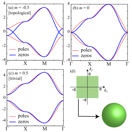
Figure 1: (a)-(c) Band dispersions (thin red lines) and zeros (thick blue lines) of the diagonal Green functions in the Hamiltonians defined in Eq. (9). For $-4<m<0$, the system becomes a topological insulator (Chern insulator) while it becomes a trivial band insulator for $m>0$. At $m=0$, the quantum phase transition between the topological insulator and the trivial band insulator can occur ($m>0$). Since the zeros traverse the bandgap, the zeros of the Green functions traverse each other in the topological insulator while they do not traverse in the trivial band insulator. (d) Brillouin zone and two-dimensional sphere. In the topological insulator with the Chern number 1, there is a mapping from the Brillouin zone to the two-dimensional sphere, which covers the two-dimensional sphere at least once.

III Two-dimensional Chern insulator (class A)

III.1 Zeros and poles in the Chern insulator

To examine the behaviors of the zeros of the Green functions in topological insulators, we employed a two-band model for a two-dimensional Chern insulator Haldane (1988) on a square lattice, defined as follows.

$$H_{\rm A}=\sum_{\nu=x,y}H_{\nu}+H_{\rm diag},$$ (6)

$$H_{\nu}=\sum_{j}h_{\nu,j},$$ (7)

$${h_{\nu,j}=c_{j+\boldsymbol{e}_{\nu}}^{\dagger}T_{\nu}c_{j}+{\rm H.c.}},$$ (8)

$$H_{\rm diag}=(2+m)\sum_{j}c_{j}^{\dagger}\sigma_{z}c_{j},$$ (9)

where $c_{j}^{\dagger}$ ($c_{j}$) represents the two-component fermion creation (annihilation) operator that is defined on the site $j$ on the square lattice spanned by two orthogonal unit vectors $\boldsymbol{e}_{\nu=x,y}$. The matrices $T_{\nu}$ are defined as

$$T_{x} =(-\sigma_{z}+{i}\sigma_{x})/2,$$ (10)

$$T_{y} =(-\sigma_{z}+{i}\sigma_{y})/2,$$ (11)

where

$$\sigma_{x}=\begin{pmatrix}0&~{}1\\ 1&~{}0\\ \end{pmatrix},\sigma_{y}=\begin{pmatrix}0&~{}-{i}\\ {i}&~{}0\\ \end{pmatrix},\sigma_{z}=\begin{pmatrix}1&~{}0\\ 0&~{}-1\\ \end{pmatrix}.$$ (13)

It is noted that the system becomes a topological (Chern) insulator for $-4<m<0$, and it becomes a trivial band insulator for $m>0$.

The Hamiltonian in the momentum space can be described as

$$H_{\rm A}(\boldsymbol{k}) =\begin{pmatrix}R_{z}(\boldsymbol{k})&R_{x}(\boldsymbol{k})-iR_{y}(\boldsymbol{k})\\ R_{x}(\boldsymbol{k})+iR_{y}(\boldsymbol{k})&-R_{z}(\boldsymbol{k})\end{pmatrix},$$ (14)

$$R_{x}(\boldsymbol{k}) =\sin{k_{x}},$$ (15)

$$R_{y}(\boldsymbol{k}) =\sin{k_{y}},$$ (16)

$$R_{z}(\boldsymbol{k}) =2+m-(\cos{k_{x}}+\cos{k_{y}}).$$ (17)

By diagonalizing the Hamiltonian, the eigenvalues (band dispersions) can be obtained as

$$E_{\pm}(\mathbf{k}) =\pm|R(\boldsymbol{k})|$$

$$=\sqrt{R_{x}(\boldsymbol{k})^{2}+R_{y}(\boldsymbol{k})^{2}+R_{z}(\boldsymbol{k})^{2}}.$$ (18)

Following the argument in Sec. II, the zeros of the Green functions are represented by the eigenvalues of the minor matrix $M_{n}$. For the 2$\times$2 matrices, the eigenvalues are the diagonal components of the Hamiltonian. Thus, the zeros of the $n$th diagonal component of the Green function ($\zeta_{n}$) are represented by

$$\zeta_{0}(\boldsymbol{k}) =M_{0}(\boldsymbol{k})=-R_{z}(\boldsymbol{k}),$$ (19)

$$\zeta_{1}(\boldsymbol{k}) =M_{1}(\boldsymbol{k})=R_{z}(\boldsymbol{k}).$$ (20)

In Fig. 1(a)-(c), a plot is presented for the band dispersions and zeros of the Green functions for several values of $m$. It was observed that the zeros of the Green function traverse each other in the topological insulator while they do not traverse in the trivial insulator. The traverse is guaranteed by the traverse of the zeros. This feature of the zeros is in sharp contrast with the band dispersions (poles of Green functions). This is because it is impossible to distinguish the topological insulator and band insulator based on only the band dispersions. When considering the standard way to identify the topological insulators, it is necessary to examine the existence of the topological invariant or the gapless edge states. However, as shown in Fig. 1, the traverse of the zeros of the Green functions in the bulk system can be used to identify the topological insulator. We note that traverses of the zeros are robust against the perturbations such as the next-nearest-neighbor transfers unless they do not destroy the topological phases. The next subsection explains how the topological invariant can guarantee the traverse and the resultant cross of the zeros of the Green functions.

III.2 Relation with the Chern number

This subsection shows that the topological invariance (Chern number $\mathcal{C}$) guarantees the traverse of the zeros in the bandgap. From the eigenvector-eigenvalue identity Eq. (5), an important relation can be obtained: a component of the eigenvector is zero ( $|\Psi_{j}^{(n)}(\boldsymbol{k})|^{2}=0$) $\leftrightarrow$ the zeros and poles of the Green function coincide ($\zeta(\boldsymbol{k})=E(\boldsymbol{k})$). These special points where $|\Psi_{j}^{(n)}|^{2}=0$ are called the vortex cores Kohmoto (1985). From the existence of such a special point, it is demonstrated how the topological invariant guarantees the traverse of the zeros. If the Chern number $\mathcal{C}$ is nontrivial, for example, $\mathcal{C}=1$, there is a one-to-one mapping from $(R_{x}(\boldsymbol{k}),R_{y}(\boldsymbol{k}),R_{z}(\boldsymbol{k}))$ to the two-dimensional sphere $S^{2}$, which covers the two-dimensional sphere at least once.

Therefore, the points in the Brillouin zone exist where $(R_{x}(\boldsymbol{k}),R_{y}(\boldsymbol{k}),R_{z}(\boldsymbol{k}))\propto(0,0,\pm 1)$. The zeros and poles coincide at these points. These points are located at $\Gamma=(0,0)$, $X=(\pi,0)$, $Y=(0,\pi)$, and $M=(\pi,\pi)$. For $R_{z}=1$ ($R_{z}=-1$), $\zeta_{0}=E_{1}$, and $\zeta_{1}=E_{0}$ ($\zeta_{0}=E_{0}$, and $\zeta_{1}=E_{1}$) occur. Thus, if $R_{z}$ takes $\pm$1 (this is guaranteed by the existence of the topological invariant), $\zeta_{0}$ traverses the band gap and crosses with $\zeta_{1}$ at least once. Therefore, the existence of the Chern number induces the traverse of the zeros in the topological insulator.

In contrast to the case of the topological insulator, when the Chern number $\mathcal{C}$ is trivial ($\mathcal{C}=0$), there exists $(R_{x}(\boldsymbol{k}),R_{y}(\boldsymbol{k}),R_{z}(\boldsymbol{k}))$ that does not completely cover the two-dimensional sphere $S^{2}$. In other words, one such point is present where $(R_{x},R_{y},R_{z})\propto(0,0,\pm 1)$ does not exist in general. In general, the zeros of the Green function do not traverse the bandgap and do not cross. It is noted that the accidental crosses of the zeroes of the Green function might occur even in trivial insulators. An example is provided in Sec. VI.3.

III.3 Gauge invariance

As demonstrated, the traverse of the zeros is guaranteed by the existence of the non-trivial topological invariant. This result indicates that the traverse of the zeros is gauge invariant. In this subsection, by explicitly performing the unitary transformation, it is established that the traverse of the zeros is gauge invariant.

By using the unitary matrix $U$, a unitary transformation is performed as follows.

$$\tilde{H}(\boldsymbol{k}) =U^{\dagger}H(\boldsymbol{k})U,$$ (21)

$$U =\begin{pmatrix}u&~{}~{}-v\\ v^{*}&~{}~{}u\end{pmatrix}$$ (22)

where $u$ is a real number, $v=v_{x}+iv_{y}$, and $u^{2}+v_{x}^{2}+v_{y}^{2}=1$. The explicit form of the transformed Hamiltonian is given as

$$\tilde{H}(\boldsymbol{k})=\begin{pmatrix}aR_{x}+bR_{y}+cR_{z}&h_{\rm off}\\ h_{\rm off}^{*}&-(aR_{x}+bR_{y}+cR_{z})\end{pmatrix},$$ (23)

where $a=2uv_{x},b=-2uv_{y},c=u^{2}-v_{x}^{2}-v_{y}^{2}$, and $h_{\rm off}=(u^{2}-v^{2})R_{x}-i(u^{2}+v^{2})R_{y}+2u(-iv_{x}+v_{y})R_{z}$. It is noted that $a^{2}+b^{2}+c^{2}=1$ is satisfied. After the unitary transformation, the zeros of the Green function are given as

$$\zeta_{0}(\boldsymbol{k}) =-(aR_{x}(\boldsymbol{k})+bR_{y}(\boldsymbol{k})+cR_{z}(\boldsymbol{k}))$$ (24)

$$\zeta_{1}(\boldsymbol{k}) =(aR_{x}(\boldsymbol{k})+bR_{y}(\boldsymbol{k})+cR_{z}(\boldsymbol{k})).$$ (25)

For $R_{x}(\boldsymbol{k})=a|R|,R_{y}(\boldsymbol{k})=b|R|,R_{z}(\boldsymbol{k})=c|R|$, the point where the zeros and poles coincide is given as $\zeta_{0}=E_{1}$ and $\zeta_{1}=E_{0}$. For the antipodal point ($R_{x}=-a|R|,R_{y}=-b|R|,R_{z}=-c|R|$), the point is given by $\zeta_{1}=E_{0}$ and $\zeta_{0}=E_{1}$. Because the existence of the topological invariant guarantees that $\boldsymbol{R}/|R|$ can cover the unit sphere, $\boldsymbol{R}$ can take $R_{x}=a|R|,R_{y}=b|R|,R_{z}=c|R|$ and the corresponding antipodal point. Thus, the traverse of the zeros of the Green function in Chern insulators is gauge invariant.

IV $\mathbb{Z}_{2}$ topological insulator in two and three dimensions (class AII)

In the previous section, as a canonical example of the topological insulators, the zeros of the Green functions in the Chern insulators were analyzed. In this section, we examine the zeros of the Green functions in the $\mathbb{Z}_{2}$ (class AII) topological insulators in two and three dimensions. It can be confirmed that the zeros traverse the bandgap in topological phases, as demonstrated in the case of the Chern insulators.

IV.1 Kane-Mele model

As an example of the $\mathbb{Z}_{2}$ topological insulators, the Kane-Mele model Kane and Mele (2005) was employed on the honeycomb lattice, which is defined as

$$H_{\rm KM} =t\sum_{\langle i,j\rangle}{\bm{c}}_{i}^{\dagger}{\bm{c}}_{j}+i\lambda_{\rm SO}\sum_{\langle\langle i,j\rangle\rangle}\nu_{ij}{\bm{c}}_{i}^{\dagger}\sigma^{z}{\bm{c}}_{j}$$

$$+\sum_{i}\Delta_{i}{\bm{c}}_{i}^{\dagger}{\bm{c}}_{i}+i\lambda_{R}\sum_{\langle i,j\rangle}{\bm{c}}_{i}^{\dagger}(\boldsymbol{\sigma}\times\frac{{\bm{d}}_{ij}}{|{\bm{d}}_{ij}|})_{z}{\bm{c}}_{j}$$

where ${\bm{c}}_{i}^{\dagger}={(c_{i\uparrow}^{\dagger},c_{i\downarrow}^{\dagger})}$ and $c_{i\sigma}^{\dagger}$ ($c_{i\sigma}$) is a creation (annihilation) operator of an electron with the spin $\sigma$ on site $i$. Each parameter is defined as follows: $t$ represents the nearest-neighbor hopping, $\lambda_{\rm SO}$ represents the spin-orbit coupling, $\Delta_{i}$ is the staggered charge potential, and $\lambda_{\rm R}$ represents the Rashba term. $\boldsymbol{\sigma}$ is defined as $\boldsymbol{\sigma}=(\sigma^{x},\sigma^{y},\sigma^{z})^{t}$ where $\sigma^{x}$, $\sigma^{y}$, and $\sigma^{z}$ are Pauli matrices. $\nu_{ij}$ is defined as $\nu_{ij}=(\boldsymbol{d}_{ik}\times\boldsymbol{d}_{kj})_{z}/|\boldsymbol{d}_{ik}\times\boldsymbol{d}_{kj}|$, where ${\bm{d}}_{ij}$ denotes the vector along two bonds that the electron traverses from site $j$ to $i$ through $k$ (see Fig. 2(a)). For simplicity, we can first assume that the Rashba term is absent ($\lambda_{R}=0$). The effects of the Rashba term are examined in the next subsection. For simplicity, $t=1$.

By performing a Fourier transformation, the Hamiltonian without the Rashba terms in the momentum space can be described as

$$H_{\sigma}(\boldsymbol{k})=\begin{pmatrix}R_{z,\sigma}(\boldsymbol{k})&R_{x}(\boldsymbol{k})-iR_{y}(\boldsymbol{k})\\ R_{x}(\boldsymbol{k})+iR_{y}(\boldsymbol{k})&-R_{z,\sigma}(\boldsymbol{k})\end{pmatrix},$$

where $R_{z,\sigma}(\boldsymbol{k})=\sigma E(\boldsymbol{k})+\Delta$ and $E(\mathbf{k})=4\lambda_{\rm SO}\sin(k_{x}/2)[\cos(k_{x}/2)-\cos(\sqrt{3}k_{y}/2)]$. $R_{x}(\boldsymbol{k})$ [$R_{y}(\boldsymbol{k})$] is defined as $R_{x}(\boldsymbol{k})={\rm Re}[E_{0}](\boldsymbol{k})$ [$R_{y}(\boldsymbol{k})={\rm Im}[E_{0}](\boldsymbol{k})$], where $E_{0}(\boldsymbol{k})=1+e^{i\boldsymbol{k}\cdot{\bm{b}}_{1}}+e^{i\boldsymbol{k}\cdot{\bm{b}}_{2}}$ [${\bm{b}}_{1}=a(1/2,\sqrt{3}/2)$,${\bm{b}}_{2}=a(-1/2,\sqrt{3}/2)$]. For this investigation, the lattice constant was set as $a=1$. By diagonalizing the Hamiltonian, the band dispersions can be obtained as

$$E_{0,\sigma}(\mathbf{k}) =\sqrt{R_{x}(\boldsymbol{k})^{2}+R_{y}(\boldsymbol{k})^{2}+R_{z,\sigma}(\boldsymbol{k})^{2}},$$

$$E_{1,\sigma}(\mathbf{k}) =-\sqrt{R_{x}(\boldsymbol{k})^{2}+R_{y}(\boldsymbol{k})^{2}+R_{z,\sigma}(\boldsymbol{k})^{2}}.$$ (26)

The zeros of the Green functions are given as

$$\zeta_{0,\sigma}(\boldsymbol{k}) =-R_{z,\sigma}(\boldsymbol{k}),$$

$$\zeta_{1,\sigma}(\boldsymbol{k}) =R_{z,\sigma}(\boldsymbol{k}).$$ (27)

In Fig. 2(b)-(d), the band dispersions and zeros of the diagonal components of the Green functions are plotted for the up spin ($E_{i,\uparrow},\zeta_{i,\uparrow}$). In the Kane-Mele model, spin-orbit coupling $\lambda_{\rm SO}$ induces the $\mathbb{Z}_{2}$ topological insulators  Kane and Mele (2005), while the staggered charge potential $\Delta$ destroys the topological insulator. By changing $\Delta$, the zeros of the Green function can be monitored in terms of how they behave in the topological and trivial insulator.

In Fig. 2(b), it is demonstrated that the zeros traverse the band gap in the $\mathbb{Z}_{2}$ topological insulator as in the Chern insulator. Because the $\mathbb{Z}_{2}$ topological insulator in the Kane-Mele model without the Rashba term is the spin Chern insulator, the traverses of the zeros are guaranteed by the existence of the spin Chern number.

By increasing the strength of the staggered charge potential $\Delta$, the insulator changes into the band insulator at $\Delta_{c}=3\sqrt{3}\lambda_{\rm SO}$. At the transition point, the crosses of the zeros are lifted at the Dirac point $K^{\prime}$ [Fig. 2(c)] and there is no traverse in the trivial insulator [Fig. 2(d)]. By using the same argument that is shown in Sec. III.3, it is demonstrated the traverse of the zeros is gauge invariant.

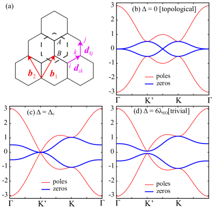
Figure 2: (a) Lattice structure and translational vectors used in the Kane-Mele model. (b)–(d) Band dispersions and the zeros of the Green functions in the Kane-Mele model ($\lambda_{\rm SO}=0.1$). The red lines display the band dispersions. The thick blue lines represent the zeros of the Green function. For simplicity, only the zeros and poles for the up spin are shown.

IV.2 Effects of Rashba term

This subsection considers the effects of the Rashba term. By adding the Rashba term, the Hamiltonian becomes $4\times 4$ and the spin Chern number is no longer well defined. The Hamiltonian with the Rashba term is given as

$$H_{\rm R}=\begin{pmatrix}R_{z,\uparrow}(\boldsymbol{k})&R_{\perp}(\boldsymbol{k})&0&z({\boldsymbol{k}}),\\ R_{\perp}(\boldsymbol{k})^{*}&-R_{z,\uparrow}(\boldsymbol{k})&w({\boldsymbol{k}})&0,\\ 0&w({\boldsymbol{k}})^{*}&R_{z,\downarrow}(\boldsymbol{k})&R_{\perp}(\boldsymbol{k}),\\ z({\boldsymbol{k}})^{*}&0&R_{\perp}(\boldsymbol{k})^{*}&-R_{z,\downarrow}(\boldsymbol{k})\end{pmatrix},$$

where $R_{\perp}(\boldsymbol{k})=R_{x}(\boldsymbol{k})-iR_{y}(\boldsymbol{k})$, and

$$z({\boldsymbol{k}}) =\sqrt{3}\lambda_{R}[(-i(1-c_{x}c_{y})+c_{x}s_{y})/\sqrt{3}+s_{x}s_{y}+is_{x}c_{y}],$$

$$w({\boldsymbol{k}}) =\sqrt{3}\lambda_{R}[(i(1-c_{x}c_{y})+c_{x}s_{y})/\sqrt{3}-s_{x}s_{y}+is_{x}c_{y}].$$

Here, we define $c_{x}$ [$s_{x}$] as $\cos(k_{x}/2)$ [$\sin(k_{x}/2)$] and $c_{y}$ [$s_{y}$] as $\cos(\sqrt{3}k_{y}/2)$ [$\sin(\sqrt{3}k_{y}/2)$]. For the Hamiltonian, because it is difficult to obtain the simple analytical form of the eigenvalues and the zeros, they were numerically obtained.

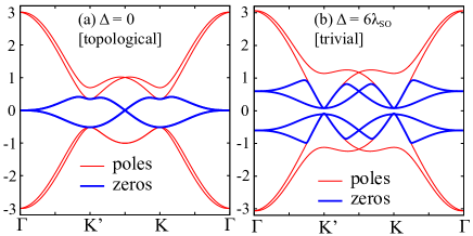
Figure 3:  Band dispersions and zeros of the Green functions in the Kane-Mele model with the Rashba term ($\lambda_{\rm SO}=0.1$ and $\lambda_{\rm R}=0.1/\sqrt{3}$) for (a) the topological insulator and (b) the trivial insulator. The red lines display the band dispersions. The thick blue lines represent the zeros of the Green function. Only the zeros of Green functions in the bandgap are presented.

Even under the existence of the Rashba term, the traverses of zeros appear in the topological insulator as shown in Fig. 3(a) while the traverses disappear in the trivial insulators occur as shown in Fig. 3(b). At the $K^{\prime}$ point, the first and fourth zeros in the bandgap coincide with the valence bands, while the second and third zeros coincide with the conduction bands. At the $K$ point, since the sign of the mass term is the opposite from the $K^{\prime}$ point, the opposite occurs. To connect each zero consistently, the first and the fourth zeros and the second and third zeros should traverse the bandgap and should cross at least once as shown in Fig. 3(a). These results indicate that the zeros of the Green function are also useful for characterizing the $\mathbb{Z}_{2}$ topological insulator.

IV.3 $\mathbb{Z}_{2}$ topological insulator in three dimensions (class AII)

This subsection considers the zeros of the Green functions in the three-dimensional topological insulators. A typical model of the three-dimensional topological insulator on the cubic lattice Qi et al. (2008); Liu et al. (2010) is given as follows.

$$R_{0} =M_{0}+3-(\cos{k_{x}}+\cos{k_{y}}+\cos{k_{z}}),$$ (28)

$$R_{1} =\sin{k_{x}},$$ (29)

$$R_{2} =\sin{k_{y}},$$ (30)

$$R_{3} =\sin{k_{z}},$$ (31)

$$H =R_{0}\alpha^{0}+R_{1}\alpha^{1}+R_{2}\alpha^{2}+R_{3}\alpha^{3}$$ (32)

$$=\begin{pmatrix}R_{0}&0&R_{3}&R_{1}-iR_{2}\\ 0&R_{0}&R_{1}+iR_{2}&-R_{3}\\ R_{3}&R_{1}-iR_{2}&-R_{0}&0\\ R_{1}+iR_{2}&-R_{3}&0&-R_{0}\\ \end{pmatrix},$$ (33)

where $\alpha^{0}=1\otimes\sigma_{z}$, $\alpha^{1}=\sigma_{x}\otimes\sigma_{x}$, $\alpha^{2}=\sigma_{y}\otimes\sigma_{x}$, and $\alpha^{3}=\sigma_{z}\otimes\sigma_{x}$. In this model, the $\mathbb{Z}_{2}$ topological insulator is achieved for $-2<M_{0}<0$ and $-6<M_{0}<-4$ while the trivial insulator is realized for $M_{0}<-6$ and $M_{0}>0$. The weak $\mathbb{Z}_{2}$ topological insulator is obtained for $-4<M_{0}<-2$. We note that this model has additional chiral symmetry because $\alpha^{4}=\alpha^{0}\alpha^{1}\alpha^{2}\alpha^{3}=1\otimes\sigma_{y}$ anticommutes with $H$ Qi et al. (2008).

The eigenvalues are given as follows.

$$E_{0} =\sqrt{R_{0}^{2}+R_{1}^{2}+R_{2}^{2}+R_{3}^{2}},$$ (34)

$$E_{1} =-\sqrt{R_{0}^{2}+R_{1}^{2}+R_{2}^{2}+R_{3}^{2}}$$ (35)

It can be noted that the eigenvalues are doubly degenerate. The zeros of the Green function in the bandgap are given as follows.

$$\zeta_{0} =-R_{0},$$

$$\zeta_{1} =R_{0}.$$ (36)

From these expressions, it can be shown that the zeros and the poles coincide at eight time-reversal points, such as the $\Gamma$, X, and Z points. To analyze the traverses of the zeros, the following was defined.

$$\eta(\boldsymbol{k})={\rm sign}(\zeta_{1}(\boldsymbol{k})).$$ (37)

If $\eta(\boldsymbol{k})=1$ ($\eta(\boldsymbol{k})=-1$) at the time reversal point, $\zeta_{1}(\boldsymbol{k})$ coincides with $E_{0}(\boldsymbol{k})$ ($E_{1}(\boldsymbol{k})$). $\eta(\boldsymbol{k})$ at the time-reversal points are shown in the inset.

Because $\zeta_{0}(\boldsymbol{k})=-\zeta_{1}(\boldsymbol{k})$, they traverse between $\eta(\boldsymbol{k})=1$ and $\eta(\boldsymbol{k})=-1$. For example, for $M_{0}=-1$ [Fig. 4(a)], they traverse between $\Gamma$ point and X point. Even for the weak topological region, they traverse as shown in Fig. 4(a) and they do not traverse in the trivial insulators. These results indicate that the traverses of the zeros can be useful for detecting the topological phases for strong and weak topological insulators since the traverses are guaranteed by the existence of the band inversions, as we detail in the next section.

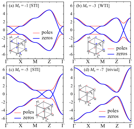
Figure 4:  Band dispersions and zeros of the Green functions in the Hamiltonian defined in Eq. (33) for (a) a strong topological insulator,  (b) a weak topological insulator,  (c) a strong topological insulator,  (d) and a trivial insulator. The red lines display the band dispersions, and the thick blue lines represent the zeros of the Green function. In the inset, $\eta(\boldsymbol{k})$ is shown for the time-reversal points. STI (WTI) is an abbreviation for a strong (weak) topological insulator.

V Relation with band inversions

In this section, we explain why the traverses of the zeros universally appear in the topological insulators. In the topological insulators, the band inversions generally occur. We denote that the occupied (unoccupied) eigenstates with the index $i\leq 0$ ($i>0$). The eigenvectors and eigenvalues are given by

$$H(\boldsymbol{k})\boldsymbol{e}_{i}(\boldsymbol{k})=E_{i}(\boldsymbol{k})\boldsymbol{e}_{i}(\boldsymbol{k}).$$ (38)

Here, $E_{0}(\boldsymbol{k})$ ($E_{1}(\boldsymbol{k})$) is the highest occupied (lowest unoccupied) eigenvalues. We assume that the band gap exists between $E_{0}$ and $E_{1}$, i.e., $E_{0}(\boldsymbol{k})<E_{1}(\boldsymbol{k})$ at any $\boldsymbol{k}$. Here, we define the band inversion as follows: A single pair of momenta $\boldsymbol{k}$, $(\boldsymbol{k}_{0},\boldsymbol{k}_{1})$ exists such that one occupied eigenvector at $\boldsymbol{k}_{1}$ [$\boldsymbol{e}_{n_{0}}(\boldsymbol{k}_{1})$] is orthogonal to all the occupied eigenvectors at $\boldsymbol{k}_{0}$, i.e.,

$$\boldsymbol{e}_{i}(\boldsymbol{k}_{0})^{\dagger}\boldsymbol{e}_{n_{0}}(\boldsymbol{k}_{1})=0~{}~{}i\in[-(N-1),0],$$ (39)

where $N$ is the number of the occupied bands. We detail the relation with the band inversion and the existence of the Chern and $Z_{2}$ topological number in Appendix B.

Then, using the eigenvectors at a certain $\boldsymbol{k}$ point ($\boldsymbol{k}=\boldsymbol{k}_{0}$), we construct the unitary matrix

$$U^{\dagger}=\begin{pmatrix}\boldsymbol{e}_{0}(\boldsymbol{k}_{0})^{\dagger}\\ \boldsymbol{e}_{1}(\boldsymbol{k}_{0})^{\dagger}\\ \boldsymbol{e}_{-1}(\boldsymbol{k}_{0})^{\dagger}\\ \boldsymbol{e}_{2}(\boldsymbol{k}_{0})^{\dagger}\\ \boldsymbol{e}_{-2}(\boldsymbol{k}_{0})^{\dagger}\\ \vdots\\ \end{pmatrix},$$ (40)

We note that the eigenvectors of the transformed Hamiltonian $\tilde{H}(\boldsymbol{k})=U^{\dagger}H(\boldsymbol{k})U$ are given by $\tilde{\boldsymbol{e}}_{i}(\boldsymbol{k})=U^{\dagger}\boldsymbol{e}_{i}(\boldsymbol{k})$. For example, the lowest two eigenvectors are transformed as

$$\tilde{\boldsymbol{e}}_{0}(\boldsymbol{k}_{0})=U^{\dagger}\boldsymbol{e}_{0}(\boldsymbol{k}_{0})=(1,0,0,\dots,0)^{t},$$ (41)

$$\tilde{\boldsymbol{e}}_{1}(\boldsymbol{k}_{0})=U^{\dagger}\boldsymbol{e}_{1}(\boldsymbol{k}_{0})=(0,1,0,\dots,0)^{t}.$$ (42)

Thus, under this unitary transformation, the zeros of the 0th (1st) component of the diagonal Green functions $\tilde{\zeta}_{0}$ ($\tilde{\zeta}_{1}$) coincide with the lowest unoccupied (highest occupied band) due to the eigenvector-eigenvalue identity Eq. (5). This situation is schematically shown in Fig. 5.

Then, we will show that the zeros of the Green function,

$${\tilde{G}=[\omega I-\tilde{H}(\boldsymbol{k})]^{-1},}$$ (43)

traverse the band gap in the topological phase, where the band inversion occurs.

Here, we assume the band inversion between $\boldsymbol{k}_{0}$ and $\boldsymbol{k}_{1}$, which is defined in Eq. (39). Without loss of generality, we can take $n_{0}=0$. Then, we obtain

$$\tilde{\boldsymbol{e}}_{0}(\boldsymbol{k}_{1})=U^{\dagger}\boldsymbol{e}_{0}(\boldsymbol{k}_{1})=(0,c,0,\dots)^{t},$$ (44)

where $c$ is a non-zero number. This illustrates that $\tilde{\zeta}_{0}$ traverses the band gap, i.e., $\tilde{\zeta}_{0}$ coincides with $E_{1}(\boldsymbol{k}_{0})$ at $\boldsymbol{k}_{0}$ and coincides with $E_{0}(\boldsymbol{k}_{1})$ at $\boldsymbol{k}_{1}$ (see Fig. 5). We can also show that $\tilde{\zeta}_{1}$ also traverses the band gap since the band inversion also occurs in the unoccupied states according to the argument given in Appendix B. This result shows the band inversion induces the traverses of the zeros in the band gap. In Appendix. C, a detailed condition for the traverse of the zeros is given. According to Eq. (126), when $\boldsymbol{e}_{0}(\boldsymbol{k}_{1})$ is orthogonal to $\boldsymbol{e}_{1}(\boldsymbol{k}_{0})$ and mainly consists of the unoccupied eigenvectors at $\boldsymbol{k}_{0}$, $\tilde{\zeta}_{0}$ traverses the band gap. We note that this condition can be regarded as a generalization of the band inversion defined in Eq. (39).

This argument demonstrates that the traverse and the resultant crosses of the zeros always appear in the topological phase by taking the unitary transformation defined in Eq. (40). As we will show in the next section, using the unitary transformation, the traverses of zeros appear in the topological insulators with chiral symmetry. Before that, we explain why the traverses of the zeros appear in the Chern insulator without taking the unitary transformation.

For the Chern insulator, the Chern number is defined as Kohmoto (1985)

$$\mathcal{C}=\sum_{n=0}^{N-1}\frac{1}{2\pi}\int_{\rm BZ}d\boldsymbol{k}[\nabla\times\boldsymbol{a}_{-n}(\boldsymbol{k})],$$ (45)

$$a_{-n}(\boldsymbol{k})=-i\boldsymbol{e}_{-n}(\boldsymbol{k})^{\dagger}\frac{\partial\boldsymbol{e}_{-n}(\boldsymbol{k})}{\partial\boldsymbol{k}}.$$ (46)

It is known if the Berry connection $a_{-n}(\boldsymbol{k})$ is smooth over the Brillouin zone, the Chern number becomes zero according to the Stokes theorem Kohmoto (1985). Therefore, if the Chern number is non-zero, the point where the phase of the eigenvector is not well defined should exist (the point is called vortex core). At that point, one component of the eigenvector becomes 0, i.e., the zeros of the Green function ($\zeta_{i}$) coincides with the eigenvalue $E_{0}$. Due to the band inversion, the same coincidence should occur for the unoccupied band, i.e., $\zeta_{i}$ coincides with $E_{1}$ at the different momentum. Therefore the zeros of the Green functions ($\zeta_{i}$) traverse the band gap. Since another zero ($\zeta_{j}$) also traverses the band gap, the zeros cross each other. This shows that the existence of the vortex core in any gauges is the reason why the traverses of the zeros appear in the Chern insulator without taking the unitary transformation. We note that the similar discussion can be applied to the four-dimensional $2\mathbb{Z}$ topological insulators (class AI) because the topological invariant is characterized by the second Chern number. In fact, as shown in Appendix D, the traverses of the zeros appear in AI topological insulator without the unitary transformation.

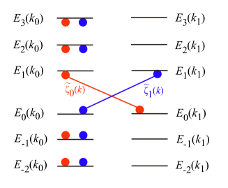
Figure 5: Schematic picture of the eigenvalues and the zeros of the Green function around the band gap under the unitary transformation defined in Eq. (40). The circles represent the points where the zeros and poles coincide. At $\boldsymbol{k}_{0}$, all the zeros coincide with the poles as shown in the left panel. If band inversions occur at $\boldsymbol{k}_{1}$, the zeros traverse the band gap as shown in the right panel. We note that the zeros outside the band gap do not necessarily coincide with the poles at $\boldsymbol{k}_{1}$. Thus, we do not show the position of the zeros outside the band gap.

VI Topological insulators with chiral symmetry (class AIII,BDI,CII)

VI.1 Choice of proper gauge

Thus far, we examined the zeros of the Green functions in the topological insulators without chiral symmetry. Here, we examine the behavior of the zeros of the Green functions in the topological insulators with chiral symmetry.

For the Hamiltonian that has chiral symmetry, the unitary matrix $\Gamma$ that anti-commutes with the Hamiltonian always exists, i.e.,

$$H\Gamma+\Gamma H=0.$$ (47)

From this, the Hamiltonian with chiral symmetry and its Green function at zero energy can be described as a block off-diagonal form as demonstrated below.

$$H=\begin{pmatrix}0&~{}~{}Q\\ Q^{\dagger}&~{}~{}0\end{pmatrix},$$ (48)

$$G(\omega=0)=-H^{-1}=\begin{pmatrix}0&~{}~{}-(Q^{\dagger})^{-1}\\ -Q^{-1}&~{}~{}0\end{pmatrix}.$$ (49)

In this representation, the unitary matrix $\Gamma$ has a diagonal form, which is given as

$$\Gamma=\begin{pmatrix}I&~{}~{}0\\ 0&~{}~{}-I\end{pmatrix}.$$ (50)

From Eq. (49), it can be observed that the zeros of the bulk Green function in the bandgap always exist at $\omega=0$ for the topological and trivial insulators. This result indicates that it is impossible to distinguish the topological phase from the trivial phases if we take the block off-diagonal form of the Hamiltonians. We also note that the vortex core is apparently absent in this gauge since the zero can not coincide with the poles if the finite gap exists. In other words, a component of the eigenvectors are always non-zero and the smooth gauge can be taken. This feature is in sharp contrast with the topological insulators without chiral symmetry such as the Chern insulators. Thus, to identify the topological phase with chiral symmetry, it is necessary to perform the proper unitary transformation. By taking the unitary transformation defined in Eq. (40), as we show later, the traverses of the zeros appear in the topological insulators with chiral symmetry because the band inversions occur in the topological phases.

VI.2 BDI and AIII topological insulators in one-dimension

As an example of the BDI and AIII topological insulators, the one-dimensional Hamiltonian Su et al. (1979); Velasco and Paredes (2017) can be considered, which is given as

$$H=\begin{pmatrix}0&R_{x}-iR_{y}\\ R_{x}+iR_{y}&0\end{pmatrix},$$ (51)

where $R_{x}=1+\gamma\cos{(x-\delta)}$ and $R_{y}=\gamma\sin{(x-\delta)}$. When $\gamma>1$ and $\delta=0$, this system becomes a topological insulator ($d=1$, BDI). If $\delta\neq 0$ and $\gamma>1$, the system becomes an AIII topological insulator Velasco and Paredes (2017).

The eigenvalues and eigenvectors of the Hamiltonian are given as follows.

$$E_{\pm}=\pm\sqrt{R_{x}^{2}+R_{y}^{2}},$$ (52)

$$\boldsymbol{e}_{\pm}=\frac{1}{\sqrt{2}}\begin{pmatrix}\frac{\alpha^{*}}{|\alpha|}\\ \pm 1\\ \end{pmatrix},$$ (53)

where $\alpha=R_{x}+iR_{y}$. Following the discussion above, by taking $k_{0}=\delta$ so as to satisfy the relation $R_{y}(k_{0})=\sin(k_{0}-\delta)=0$, the unitary transformation is given by

$$U^{\dagger}=\begin{pmatrix}\boldsymbol{e}_{-}(k_{0})^{\dagger}\\ \boldsymbol{e}_{+}(k_{0})^{\dagger}\end{pmatrix}=\frac{1}{\sqrt{2}}\begin{pmatrix}1&~{}~{}-1\\ 1&~{}~{}1\\ \end{pmatrix}.$$ (54)

Using the unitary matrix, the transformed Hamiltonian is obtained as follows.

$$\tilde{H}=U^{\dagger}HU=\begin{pmatrix}R_{x}&~{}~{}iR_{y}\\ -iR_{y}&~{}~{}-R_{x}\end{pmatrix}.$$ (55)

The zeros of the Green function for the transformed Hamiltonian $\tilde{H}$ are given as follows.

$$\tilde{\zeta}_{0} =-R_{x},$$

$$\tilde{\zeta}_{1} =R_{x}.$$ (56)

For the BDI topological insulator ($\delta=0,\gamma>1$), the zeros traverse the bandgap as shown in Fig. 6(a) whereas the zeros do not traverse in the trivial insulator. It can be confirmed that the same behavior occurs in the AIII topological insulators as shown in Fig. 6(c).

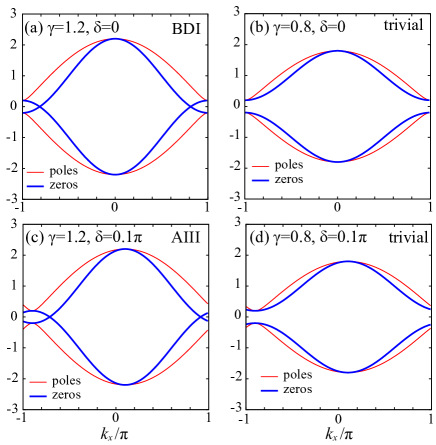
Figure 6:  Band dispersions and zeros of the Green functions in the model Hamiltonian for (a),(b) BDI, and (c),(d) AII topological insulators, which is defined in Eq. (51). The red lines display the band dispersions, and the thick blue lines represent the zeros of the Green function. The zeros traverse the bandgap for the BDI and AIII topological insulators.

VI.3 CII topological insulator in one-dimension

As an example of the CII topological insulators, the following four-orbital models were applied Liu et al. (2019).

$$H=\begin{pmatrix}0&~{}~{}0&~{}~{}R_{x}&~{}~{}iA+R_{y}\\ 0&~{}~{}0&~{}~{}iA+R_{y}&~{}~{}R_{x}\\ R_{x}&~{}~{}-iA+R_{y}&~{}~{}0&~{}~{}0\\ -iA+R_{y}&~{}~{}R_{x}&~{}~{}0&~{}~{}0\end{pmatrix},$$ (57)

where $R_{x}=t_{\perp}$, $R_{y}=2t\sin{k_{x}}$, and $A=s+2s^{\prime}\cos{k_{x}}$. When $(t_{\perp}/t)^{2}+(s/s^{\prime})^{2}<4$, this system becomes a topological insulator ($d=1$, CII). The eigenvalues of the Hamiltonian are given as follows.

$$E_{0} =-\sqrt{(R_{x}+R_{y})^{2}+A^{2}},$$ (58)

$$E_{1} =-\sqrt{(R_{x}-R_{y})^{2}+A^{2}},$$ (59)

$$E_{2} =\sqrt{(R_{x}-R_{y})^{2}+A^{2}},$$ (60)

$$E_{3} =\sqrt{(R_{x}+R_{y})^{2}+A^{2}}.$$ (61)

Following the discussion above, by tanking $k_{0}=0$, we obtain the unitary matrix by numerically diagonalizing the Hamiltonian. Using the unitary matrix, we numerically obtain the zeros of the Green function of $\tilde{H}=U^{\dagger}HU$. The zeros are shown in Fig. 7. We note that the eigenstates are degenerate at $k=0$ and the form of the unitary transformation is not unique. Nonetheless, the traverses of the zero are guaranteed by the existence of the band inversion as we showed above.

As illustrated in Fig. 7(a), in the CII topological insulator, the zeros of the Green functions traverse the bandgap. Basically, the crosses vanish in the trivial insulator sufficiently away from the transition point. However, the accidental crosses of the zeros still survive, even in the trivial insulators as shown in Fig. 7(c) near the transition point. These crosses are not guaranteed by the traverse of the zeros and we can remove the accidental crosses without gap closing.

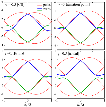
Figure 7:  Band dispersions and zeros of the Green functions in the model of the CII topological insulators for the (a) topological insulator,  (b) transition point,  (c) trivial insulator near the phase transition,  (d) and the trivial insulator. For this investigation, $t=1,s=s^{\prime}=1$, and $t_{\perp}=\sqrt{4-(s/s^{\prime})^{2}}+\gamma$. For $\gamma<0$ ($\gamma>0$), the system becomes a topological (trivial) insulator. The red lines display the band dispersions, and the thick blue lines represent the zeros of the Green function.

VII Higher-order topological insulators

As demonstrated in the previous sections, the zeros traverse in the topological insulators because the gapless edge states inevitably induce the traverse of the zeros. Recently, new classes of the topological insulators have been found, such as the higher-order topological insulators Benalcazar et al. (2017); Schindler et al. (2018). In the higher-order topological insulators in $n$ dimensions, the gapless edge states appear below $n-2$ dimensions. For example, the three-dimensional higher-order topological insulators have one-dimensional edge states and the two-dimensional higher-order topological insulators have zero-dimensional edge states. In this section, we demonstrate that the traverses of the zeros in the bulk system also appear in the higher-order topological insulators because the band inversion occurs.

VII.1 Higher-order topological insulators in three dimensions

A model of the three-dimensional higher-order topological insulator on the cubic lattice is described as follows Schindler et al. (2018).

$$R_{0} =M+(\cos{k_{x}}+\cos{k_{y}}+\cos{k_{z}}),$$ (62)

$$R_{1} =\sin{k_{x}},$$ (63)

$$R_{2} =\sin{k_{y}},$$ (64)

$$R_{3} =\sin{k_{z}},$$ (65)

$$R_{4} =\Delta_{2}(\cos{k_{x}}-\cos{k_{y}}),$$ (66)

$$H =R_{0}\alpha^{0}+R_{1}\alpha^{1}+R_{2}\alpha^{2}+R_{3}\alpha^{3}+R_{4}\alpha^{4}$$ (67)

$$=\begin{pmatrix}R_{0}&~{}0&R_{3}-iR_{4}&~{}R_{1}-iR_{2}\\ 0&~{}R_{0}&R_{1}+iR_{2}&~{}-R_{3}-iR_{4}\\ R_{3}+iR_{4}&~{}R_{1}-iR_{2}&-R_{0}&~{}0\\ R_{1}+iR_{2}&~{}-R_{3}+iR_{4}&0&~{}-R_{0}\\ \end{pmatrix}$$ (68)

The eigenvalues are given as

$$E_{0} =\sqrt{R_{0}^{2}+R_{1}^{2}+R_{2}^{2}+R_{3}^{2}+R_{4}^{2}},$$ (69)

$$E_{1} =-\sqrt{R_{0}^{2}+R_{1}^{2}+R_{2}^{2}+R_{3}^{2}+R_{4}^{2}},$$ (70)

and the zeros are given as

$$\zeta_{0} =-R_{0},$$ (71)

$$\zeta_{1} =R_{0}.$$ (72)

It can be noted that without $R_{4}$, this model is the same as that of the three-dimensional $\mathbb{Z}_{2}$ topological insulators defined in Eq. (33). It is shown that the system changes from the $\mathbb{Z}_{2}$ topological insulator into a higher-order topological insulator when $R_{4}$ is added  Schindler et al. (2018).

As shown in Fig. 8, the traverses of the zeros exist even for the higher-order topological insulators. Although $R_{4}$ lifts the coincidences of the zeros and poles at some $k$ points such as X, the coincidences still exist for $\Gamma$, M, and Z. This indicates that the band inversion still remains in the higher-order topological insulators.

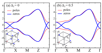
Figure 8:  Band dispersions (thin red curves) and zeros (thick blue curves) of the Green functions in the model Hamiltonians for the three-dimensional higher-order topological insulators defined in Eq. (68). For (a)$\Delta_{2}=0$, the system is a $\mathbb{Z}_{2}$ topological insulator and the system becomes HOTI for (b) $\Delta_{2}=0.5$.

VII.2 Higher-order topological insulators in two dimensions

As an example of the two-dimensional higher-order topological insulators Benalcazar et al. (2017), we consider the following Hamiltonian.

$$H =$$

$$\begin{pmatrix}0&0&~{}iR_{z}+A&iR_{x}+R_{y}\\ 0&0&~{}iR_{x}-R_{y}&-iR_{z}+A\\ -iR_{z}+A&-iR_{x}-R_{y}&~{}0&0\\ -iR_{x}+R_{y}&iR_{z}+A&~{}0&0\end{pmatrix}$$ (73)

where $R_{x}=E\sin{k_{y}}$, $R_{y}=\gamma+E\cos{k_{y}}$, $R_{z}=E\sin{k_{x}}$, and $A=\gamma+E\cos{k_{x}}$. The eigenvalues are given as

$$E_{0,\pm} =\pm\sqrt{A^{2}+R_{x}^{2}+R_{y}^{2}+R_{z}^{2}},$$ (74)

$$E_{1,\pm} =\pm\sqrt{A^{2}+R_{x}^{2}+R_{y}^{2}+R_{z}^{2}}.$$ (75)

We note that the eigenvalues are doubly degenerate.

Because the system has chiral symmetry, according to the procedure described above, we define the following unitary matrix by taking $\boldsymbol{k}_{0}=(0,0)$.

We show zeros of the Green functions of transformed Hamiltonian $\tilde{H}=U^{\dagger}HU$ in Fig. 9. We find that the zeros traverse the band gap in the higher-order topological insulator while they do not traverse in the trivial insulator. This result indicates that the traverse of the zeros in the bulk system is useful even for detecting the higher-order topological phases.

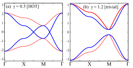
Figure 9:  Band dispersions (thin red curves) and zeros (thick blue curves) of the Green functions in the model for two-dimensional higher-order topological insulators for (a) $\Gamma=0.5$ and (b) $\Gamma=1.2$.

VII.3 Higher-order topological insulator in the Fu-Kane-Mele model under a magnetic field

Finally, we examine how the zeros of the Green functions behave in the Fu-Kane-Mele model under a magnetic field Fu et al. (2007); Fu_PRB2007; Turner et al. (2010), which is defined as follows.

$$R_{1} =1+\delta t_{1}+[\cos{k_{1}}+\cos{k_{2}}+\cos{k_{3}}],$$ (76)

$$R_{2} =\sin{k_{1}}+\sin{k_{2}}+\sin{k_{3}},$$ (77)

$$R_{3} =\lambda_{\rm SO}[\sin{k_{2}}-\sin{k_{3}}-\sin{(k_{2}-k_{1})}+\sin{(k_{3}-k_{1})}],$$ (78)

$$R_{4} =\lambda_{\rm SO}[\sin{k_{3}}-\sin{k_{1}}-\sin{(k_{3}-k_{2})}+\sin{(k_{1}-k_{2})}],$$ (79)

$$R_{5} =\lambda_{\rm SO}[\sin{k_{1}}-\sin{k_{2}}-\sin{(k_{1}-k_{3})}+\sin{(k_{2}-k_{3})}],$$ (80)

$$H =\begin{pmatrix}R_{5}+h_{z}&~{}R_{1}-iR_{2}&R_{3}-iR_{4}&~{}0\\ R_{1}+iR_{2}&~{}-R_{5}+h_{z}&0&~{}-R_{3}+iR_{4}\\ R_{3}+iR_{4}&~{}0&-R_{5}-h_{z}&~{}R_{1}-iR_{2}\\ 0&~{}R_{3}-iR_{4}&R_{1}+iR_{2}&~{}R_{5}-h_{z}\\ \end{pmatrix},$$ (81)

where $k_{1}=(k_{y}+k_{z})/2$, $k_{2}=(k_{x}+k_{z})/2$,  $k_{3}=(k_{x}+k_{y})/2$, and $h_{z}$ represent the magnetic field.

It is shown that the three-dimensional $\mathbb{Z}_{2}$ topological insulator appears in the Fu-Kane-Mele model. The gapless surface states are gapped out when the magnetic field is applied because the magnetic field breaks the time-reversal symmetry. Nevertheless, by analyzing the entanglement spectrum, Turner $et$ $al$. showed that the topological properties of the systems still remain Turner et al. (2010). They demonstrated that the entanglement spectrum behaves as gapless surface states, even under a magnetic field. Recently, it has been established that the one-dimensional hinge states appear in the $\mathbb{Z}_{2}$ topological insulator under a magnetic field Matsugatani and Watanabe (2018); Fang and Fu (2019). The higher-order topological nature may be the origin of the characteristic behavior in the entanglement spectrum. Here, we show that the zeros of the Green functions can also capture the topological properties of this system.

In Fig. 10(a) and (b), the bulk band dispersions and the zeros of the Green functions for $h_{z}=0$ and $h_{z}=0.2$, respectively, are presented. For this investigation, $\delta t=0.5$ and $\lambda_{\rm SO}=0.25$. For visibility, we perform the unitary transformation that consists of the eigenvectors at $\Gamma$ point. Even under the finite magnetic field, it was determined that the traverses of the zeros of the Green functions can still survive.

To observe the surface/edge states, the two-dimensional surface states and the one-dimensional hinge states were calculated in Fig. 10(c)-(f). As shown in Fig. 10(d), the gapless surface states are gapped out by the magnetic field. However, as shown in Fig. 10(f), the gapless one-dimensional edge (hinge) states appear under the magnetic field. This result shows that a higher-order topological insulator is realized in the Fu-Kane-Mele model under the magnetic field and is captured by the traverses of the zeros.

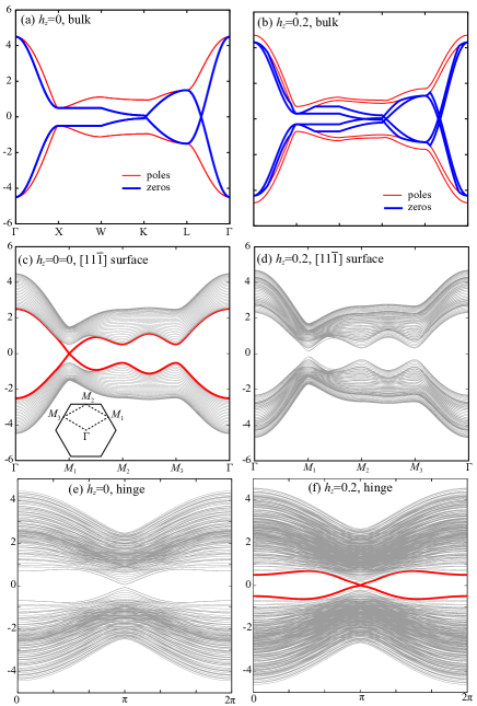
Figure 10:  Band dispersions (thin red curves) and zeros (thick blue curves) of the Green functions in the Fu-Kane-Mele model for (a) $h_{z}=0$ and (b) $h_{z}=0.2$. For this study, $\delta t=0.5$ and $\lambda_{\rm SO}=0.25$. The traverses of the zeros survive even under finite magnetic fields.  Band dispersions in the slab geometry ([11$\bar{1}$] surface) in the Fu-Kane-Mele model for (c) $h_{z}=0$ and (d) $h_{z}=0.2$. Surface states (thick red curves shown in (c)) are gapped out by the magnetic field.  Band dispersions in the hinge geometry in the Fu-Kane-Mele model for (e) $h_{z}=0$ and (f) $h_{z}=0.2$. Gapless hinge states appear for $h_{z}=0.2$. The unit vectors were employed as $\boldsymbol{a}_{1}=(0,1,1)$, $\boldsymbol{a}_{2}=(1,0,1)$, and $\boldsymbol{a}_{3}=(1,1,0)$. To realize the [11$\bar{1}$] surface (the one-dimensional hinge state), the periodicity was cut for $\boldsymbol{a}_{3}$ ($\boldsymbol{a}_{2}$ and $\boldsymbol{a}_{3}$). The calculations of the surface and hinge states were performed using PythTB Pyt .

VIII Relation with edge states

The traverse and the resultant cross of the zeros resemble the gapless edge modes, which appear in the topological insulators. This section shows that the traverse of the zeros of the Green functions has a relation with the gapless edge state, i.e., degeneracies of the eigenvalues of the edge Hamiltonian guarantee the existence of the zeros’ surface in the band gap. We note that this argument is applicable to the Hamiltonians only with the nearest-neighbor hoppings. For the Hamiltonian with further-neighbor hoppings, the argument can not be directly applied.

We consider the two-dimensional Chern insulators as an example, which is defined in Eq. (9). We rewrite the Hamiltonians in the real space for the $x$ direction (the length is set to $L$) as

$$H_{L}(p)=\begin{pmatrix}h_{0}~{}~{}&h_{x}~{}~{}&0~{}~{}&\ldots~{}~{}&0~{}~{}&p\times h_{-x}\\ h_{-x}~{}~{}&h_{0}~{}~{}&h_{x}~{}~{}&0~{}~{}&0~{}~{}&0\\ 0~{}~{}&h_{-x}~{}~{}&h_{0}~{}~{}&h_{x}~{}~{}&0~{}~{}&0\\ \vdots~{}~{}&\vdots~{}~{}&\ddots~{}~{}&\ddots~{}~{}&\ddots~{}~{}&\vdots\\ 0~{}~{}&0~{}~{}&0~{}~{}&h_{-x}~{}~{}&h_{0}~{}~{}&h_{x}\\ p\times h_{x}~{}~{}&0~{}~{}&0~{}~{}&0~{}~{}&h_{-x}~{}~{}&h_{0}\end{pmatrix},$$ (82)

$$h_{0}=\begin{pmatrix}2+m-\cos{k_{y}}~{}~{}&-i\sin{k_{y}}\\ i\sin{k_{y}}~{}~{}&-(2+m)+\cos{k_{y}}\end{pmatrix},$$ (83)

$$h_{x}=\begin{pmatrix}1/2~{}~{}&i/2\\ i/2~{}~{}&-1/2\\ \end{pmatrix},$$ (84)

$$h_{-x}=\begin{pmatrix}1/2~{}~{}&-i/2\\ -i/2~{}~{}&-1/2\end{pmatrix},$$ (85)

where $p$ is the scholar value and controls the boundary conditions. For example, the open-boundary condition corresponds to $p=0$, and the periodic-boundary condition corresponds to $p=1$. We note that the periodic Hamiltonian ($p=1$) includes the $L-1$ edge Hamiltonian

$$H_{L}(p=1)=\begin{pmatrix}h_{0}~{}~{}~{}~{}&B\\ B^{\dagger}~{}~{}~{}~{}&H_{L-1}(p=0)\end{pmatrix},$$ (86)

where $B=(h_{x},0,\ldots,0,p\times h_{-x})$. For simplicity, we denote $H_{\rm real}(k_{y})=H_{L}(p=1,k_{y})$ and $H_{\rm edge}(k_{y})=H_{L-1}(p=0,k_{y})$. We note the relation between the edge states and the minor matrix are studied in the context of the Hermiticity of the tight-binding Hamiltonian operators Fukui (2020).

Here, we define the partial Fourier transformed Green function as

$$\bar{G}_{n}(k_{y},\omega)=\int_{-\pi}^{\pi}G_{n}(k_{x},k_{y},\omega)dk_{x}.$$ (87)

We note that $\bar{G}_{n}$ is the Green functions of $H_{\rm real}(k_{y})$, i.e.,

$$\bar{G}_{n}(k_{y},\omega)=[\omega-H_{\rm real}(k_{y})]^{-1}.$$ (88)

From this definition, if $\bar{G}_{n}(k_{y},\omega)$ becomes zero, the following relation is satisfied.

$$\bar{G}_{n}(k_{y},\omega)=\int_{-\pi}^{\pi}G_{n}(k_{x},k_{y},\omega)dk_{x}=0.$$ (89)

This indicates that the $G_{n}(k_{x},k_{y},\omega)$ changes its sign as a function of $k_{x}$.

The zeros of $\bar{G}_{n}(k_{y},\omega)$ are given by the eigenvalues of the minor matrix $M_{n}$ of $H_{\rm real}(k_{y})$. Based on the periodicity, we only consider the eigenvalues of $M_{0}$ and $M_{1}$. Because $M_{0}$ and $M_{1}$ include the edge Hamiltonian, $H_{\rm edge}$ can be regarded as a minor matrix of $M_{0}$ and $M_{1}$. Thus, from the Cauchy interlacing identity (see Appendix E and F), the eigenvalues of $H_{\rm edge}$ are located between the eigenvalues of $M_{0}$ and $M_{1}$ and vice versa. This relation can be expressed as

$$E_{i-1}(H_{\rm edge})\leq E_{i}(M_{0})=\bar{\zeta}_{0}(H_{\rm real})\leq E_{i}(H_{\rm edge}),$$

$$E_{i-1}(H_{\rm edge})\leq E_{i}(M_{1})=\bar{\zeta}_{1}(H_{\rm real})\leq E_{i}(H_{\rm edge}).$$ (90)

If the eigenvalues of the edge Hamiltonian are doubly degenerate, the zeros of the bulk Hamiltonian should coincide, i.e.,

$$\bar{\zeta}_{0}(H_{\rm real})=\bar{\zeta}_{1}(H_{\rm real}).$$ (91)

This indicates that the gapless edge states (they cross in the bandgap) inevitably induce the degeneracy of the zeros in $\bar{G}_{n}$.

Using numerical calculations, we demonstrate the application of this argument to the Chern insulators. In Fig. 12, the poles of the zeros of the Green functions for the periodic Hamiltonian $H_{L=20}(p=1)$ are defined in Eq. (82) for $m=-0.5$. We also show the poles of the edge Hamiltonian (edge states) for $H_{L=19}(p=0)$. We can confirm that the zeros of the periodic Hamiltonian exist between the poles of the edge Hamiltonian, and they degenerate when the poles of the edge Hamiltonian cross ($k_{y}=0$).

In general, for the $m$-orbital system (the size of $h_{0}$ is $m\times m$), it can be shown that the $m$-fold degeneracy in the edge states (gapless edge states) induces the $m$-fold degeneracy in the zeros of $\bar{G}$. The proof of this statement is shown in Appendix E and F. However, because the proof is based on the Cauchy interlacing inequality, it can not be applied to the Hamiltonian with the further-neighbor hoppings, where degeneracy of the edge states ($m_{\rm edge}$) is less than the number of orbitals ($m_{\rm orb}$), i.e., $m_{\rm edge}<m_{\rm orb}$. For example, if we introduce the next-nearest neighbor hopping, the size of $h_{0}$ becomes $4\times 4$ while the degeneracy of the edge states still remains $2$. In this situation, the Cauchy interlacing inequality can not be applied and the degeneracy of the edge states does not necessarily induce the degeneracy in the zeros of $\bar{G}$.

Here, we argue how the traverses of the zeros in $\bar{G}$ are related with the zeros of the Green functions in the momentum space. We first consider the region where the $\omega$ is negative ($\omega<0$) and the 0th component of the Green function ($\bar{G}_{0}$ and $G_{0}$). For $\omega<0$, at the certain $k_{y}=\pm k_{0}$, $\bar{G}_{0}(k_{y},\omega)$ becomes 0. This indicates that the finite positive and negative regions exist in the original Green functions at $\pm k_{0}$ according to Eq. (89). Since the positive and negative regions do not immediately vanish even if we adiabatically change $k_{y}$, the zero’s surface exists in the original Green functions $G_{0}$ as shown in Fig. 12(a).

At $\omega=0$, $\bar{G}_{0}(k_{y},\omega)$ becomes 0 at $k_{y}=0$. This also indicates the existence of the zero’s surface around $k_{y}=0$ (see Fig. 12 (b)). We also note that the zero’s surface can not immediately vanish even if we change $\omega$, the zero’s surface survives for $\omega>0$ as is shown Fig. 12 (c). From this consideration, we can say that the zero’s surface of $G_{0}$ exists at least for $\omega\leq 0$

The opposite thing occurs for $G_{1}$ and $\bar{G}_{1}$, i.e., the zero’s surface exists at least for $\omega\geq 0$. These results indicate that the zeros’ surfaces exist in the band gap if the gapless edge states exist. This means that at least one diagonal component of the Green functions becomes zero in the band gap due to the existence of the gapless edge states. The existence of the zeros’ surface is consistent with the existence of the traverses of the zeros in the bulk Green functions. We note that, however, the traverses of the zeros are not guaranteed by the degeneracy of the zeros of $\bar{G}$.

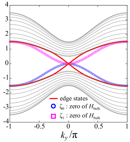
Figure 11:  Band dispersions (thin black curves) and zeros of the Green functions (blue circles and magenta squares) for the bulk Hamiltonian $H_{\rm reak}(k_{y})$. For this investigation, $L=20$ and $m=-0.5$. The zeros of the Green function are plotted in the bandgap. It is also established that the eigenvalues (thick red curves) of $H_{\rm edge}(k_{y})$ are in the bandgap. As described in the main text, the cross of the eigenvalues of $H_{\rm edge}(k_{y})$ induces the cross of the zeros in the partially Fourier transformed Green functions $\bar{G}_{0}(k_{y},\omega)$.

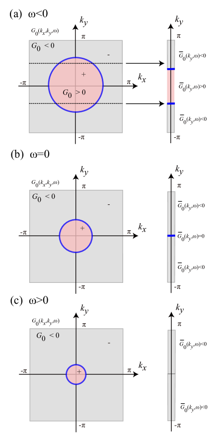
Figure 12:  Sign of the Green functions of $G_{0}(k_{x},k_{y},\omega)$ (left panel) and the partially Fourier transformed Green functions ($\bar{G}_{0}(k_{y},\omega)$) (right panel) for (a) $\omega>0$, (b) $\omega=0$, and (c) $\omega<0$. The zeros of the Green functions are denoted by the thick (blue) lines.

IX Summary

In summary, this study focused on the zeros of the diagonal components of the Green functions in topological insulators. Based on the arguments that were used in the eigenvector-eigenvalue identity Denton et al. (2022), it was first demonstrated that the zeros of the diagonal components of the Green functions are given by the eigenvalues of the minor matrix $M_{n}$, which is obtained by removing the $n$th row and column from the original Hamiltonian. This mathematical foundation offers an efficient way to study the zeros of the Green functions both analytically and numerically. We have also shown that the zeros can visualize the information of the band inversions via the eigenvector-eigenvalue identity.

For a two-dimensional Chern insulator, which is a canonical model of two-dimensional a topological insulator, it is established that the traverse of the zeros is a key to distinguishing topological insulators from trivial insulators. For the Chern insulators, this study has explicitly shown that the existence of the Chern number guarantees the traverse of the zeros in bulk systems. It has been demonstrated that the traverse of the zeros is gauge invariant, although the positions of the zeros are not. It is observed that the traverses of the zeros can occur in the other class of the topological insulators without chiral symmetries such as the $\mathbb{Z}_{2}$ (class AII) topological insulators in two and three dimensions and $2\mathbb{Z}$ (class AI) topological insulators in four dimensions.

We give a general argument that the band inversions induce the traverses of the zeros in the band gap. Since the band inversions occur in topological phases, the traverses of the zeros universally occur in the topological phase. This argument also shows that the traverse of the zeros always occur if we take the proper unitary transformation. The unitary transformation is used for identifying the topological phase with chiral symmetry.

For topological insulators with chiral symmetry, this study demonstrated that the zeros also traverse the bandgap when we take the suitable unitary transformation defined in Eq. (40). By taking the model Hamiltonians for class BDI, AIII, and CII topological insulators, this investigation has shown that the traverses of the zeros always occur in topological phases.

Since the traverses of the zeros are guaranteed by the existence of the band inversions it is expected that this is useful for detecting other exotic topological phases, which are not listed in the conventional periodic table for topological insulators (Table  1). As an example of these exotic topological phases, we consider the higher-order topological insulators. The traverse of the zeros is also useful for detecting the higher-order topological insulators in two and three dimensions.

We also show that the gapless edge states guarantee the existence of the zeros’ surface in the band gap for the Hamiltonian with the nearest neighbor hoppings. Although the relation with the edge states and the behavior of the zeros in the bulk system can be proved only for the limited case, this result implies that the zeros have close relation with the edge states and offers another point of view of the bulk edge-correspondence Hatsugai (1993).

The comprehensive analysis in this study demonstrates that the zeros of the Green functions can be used as a simple visual detection tool for topological phases via the band inversions. It may be useful when searching for new topological phases because the traverses of the zeros can be easily detected without any assumptions. In addition, since this method does not require full gap states but only needs the traverse of the zeros, the zeros of the Green functions can be useful to identify the exotic topological semimetals such as the Weyl Shindou and Nagaosa (2001); Murakami (2007); Wan et al. (2011); Burkov (2018) and the Topological Dirac semimetals Wang et al. (2012a); Morimoto and Furusaki (2014); Yang and Nagaosa (2014).

It needs to be noted that the accidental crosses of the zeros in the trivial phases may occur, as demonstrated for the CII topological insulator. We want to emphasize that this type of cross is not protected by the traverse of the zeros, i.e., the band inversion. By visualizing the behavior of the zeros in the band gap, it is easy to distinguish whether the crosses of the zero are accidental or not. We also note that the accidental crosses appear in the Rice-Mele model Rice and Mele (1982); Xiao et al. (2010), which has non-topological edge states. In the Rice-Mele model, since the zeros do not traverse the band gap either, we can distinguish whether the crosses are accidental. Thus, the traverse of the zeros of the Green functions is useful when searching for the topological phases since the absence of the traverses indicates that the system is not topological in the sense that they have no band inversions. This fact may be useful in the screening process for searching the topological materials by combining with the high-throughput $ab$ $initio$ calculations Zhang et al. (2019); Tang et al. (2019b); Vergniory et al. (2019); Xu et al. (2020).

In this paper, the rediscovered eigenvector-eigenvalue identity is essentially used for showing the existence of the traverse of the zeros due to the band inversion. Since the band inversion universally occurs in the topological phases, the traverse of the zeros offers a useful guideline for identifying the topological phases. Thus, our paper gives a direct application of the eigenvector-eigenvalue identity in condensed matter physics, which is a fundamental relation in linear algebra but has long been overlooked.

This study was restricted to the analysis of topological insulators for simplicity; however, a similar analysis is possible for topological superconductors, where the band inversion also occurs. It is known that several topological superconductors can be mapped to the models of the topological insulators,e.g., the model for the class D topological superconductors in the two dimension is mapper to the model for the Chern insulator Wang et al. (2021). In those systems, the traverses zeros also appear in the topological superconductors. Furthermore, a similar analysis might be possible for the disordered Li et al. (2009); Kobayashi et al. (2013) and interacting Gurarie (2011); Wang et al. (2012b); Witczak-Krempa et al. (2014) systems because the Green functions for the correlated and/or disordered systems are well-defined. We note that zeros of the Green functions in correlated electron systems are recently studied using dynamical mean-field theory Tran et al. (2022). These unexplored issues are intriguing but need to be further investigated.

Appendix A Proof of the Cauchy interlacing inequalities

Although the proof of the Cauchy interlacing inequalities is shown in the literature Wilkinson (1963); Hwang (2004), we have provided another proof of the inequalities based on the structure of the Green functions to make this paper self-contained. To prove the Cauchy interlacing inequalities, the definition of the Green function (Eq. (2)) is rewritten as

$$G_{n}(\boldsymbol{k},\omega) =\frac{N_{n}(\boldsymbol{k},\omega)}{\prod_{i}{(\omega-E_{i})}},$$ (92)

$$N_{n}(\boldsymbol{k},\omega) =\sum_{j}|\Psi_{j}^{(n)}|^{2}\prod_{i\neq j}(\omega-E_{i}).$$ (93)

The roots of the ($n-1$)th polynomial $N_{n}(\boldsymbol{k},\omega)$ correspond to the zeros of $G_{n}(\boldsymbol{k},\omega)$, i.e., the eigenvalues of the minor matrix $M_{n}({\boldsymbol{k}})$.

From Eq. (93), it can be shown that $N_{n}(\boldsymbol{k},\omega)$ changes its sign between $E_{i}(\boldsymbol{k})$ and $E_{i+1}(\boldsymbol{k})$, i.e., $N_{n}(\boldsymbol{k},E_{i}(\boldsymbol{k}))\cdot N_{n}(\boldsymbol{k},E_{i+1}(\boldsymbol{k}))<0$ unless $|\Psi^{(n)}_{i}|=0$ or $|\Psi^{(n)}_{i+1}|=0$. This indicates that the $N_{n}(\boldsymbol{k},\omega)$ has at least one real root between $E_{i}(\boldsymbol{k})$ and $E_{i+1}(\boldsymbol{k})$. Because the $N_{n}(\boldsymbol{k},\omega)$ is the ($n-1$)th polynomial with respect to $\omega$, the number of roots between $E_{i}(\boldsymbol{k})$ and $E_{i+1}(\boldsymbol{k})$ should be one. For $|\Psi^{(n)}_{i}(\boldsymbol{k})|=0$, $\omega=E_{i}(\boldsymbol{k})$ is a root of $N_{n}(\boldsymbol{k},\omega)$. This is consistent with the eigenvector-eigenvalue identity.

Thus, for both $|\Psi_{i}^{(n)}|=0$ and $|\Psi_{i}^{(n)}|\neq 0$, $N_{n}(\boldsymbol{k},\omega)$ has one real root between $E_{i}(\boldsymbol{k})$ and $E_{i+1}(\boldsymbol{k})$. In other words, one zero of $G_{n}(\boldsymbol{k},\omega)$ should exist between every adjacent eigenvalue (poles of the Green function). This was also pointed out in a previous study  Seki and Yunoki (2017). This represents the Cauchy interlacing inequalities.

Appendix B Relation between the band inversion and the topological invariants

Let $\boldsymbol{e}_{i}(\boldsymbol{k})$ is the $i$th eigenvectors of Hamiltonian $H(\boldsymbol{k})$. We take $N$ ($M$) as the number of the occupied (unoccupied) states. We define the overlap matrix $U$ as

$$U(\boldsymbol{k}_{0},\boldsymbol{k}_{1})=\mathcal{E}(\boldsymbol{k}_{0})^{\dagger}\mathcal{E}(\boldsymbol{k}_{1}),$$ (94)

where $\mathcal{E}(\boldsymbol{k})$ is the set of the eigenvectors at $\boldsymbol{k}$,

$${\mathcal{E}(\boldsymbol{k})=[\boldsymbol{e}_{0}(\boldsymbol{k}),\boldsymbol{e}_{1}(\boldsymbol{k}),\dots,\boldsymbol{e}_{N+M-1}(\boldsymbol{k})]}.$$ (95)

Since $\mathcal{E}(\boldsymbol{k})$ is unitary, $U$, which is a product of two unitary matrices, is also unitary. For the unitary matrix $U$, we consider the following block matrix representation:

$$U=\begin{pmatrix}U_{11}~{}~{}&U_{12}\\ U_{21}~{}~{}&U_{22}\end{pmatrix},$$ (96)

where $U_{11}$ ($U_{22}$) is the overlap matrix for the occupied (unoccupied) states and it is the $N\times N$ ($M\times M$) unitary matrix while $U_{12}$ ($U_{21}$) is the $N\times M$ ($M\times N$) overlap matrix between the occupied and unoccupied states. We note that $\det{U_{11}}$ is a key quantity for identifying the non-trivial Chern and $Z_{2}$ topological insulators. When a system is the non-trivial Chern or $Z_{2}$ topological insulator, there exists, at least, a single pair of $\boldsymbol{k}$, $(\boldsymbol{k}_{0},\boldsymbol{k}_{1})$, that satisfies $\det{U_{11}}=0$.

For the Chern insulator, it is shown that, if $\det{U_{11}}=0$ holds at a pair of momenta, $(\boldsymbol{k}_{0},\boldsymbol{k}_{1})$, irrespective of the choice of the gauge, the gauge fixing is impossible Hatsugai (2004). Thus, if $\det{U_{11}}=0$ holds at a pair of momenta, there is a non-trivial Chern number.

In the $Z_{2}$ topological insulators Kane and Mele (2005); Fukui and Hatsugai (2007), it is also shown that the non-trivial $Z_{2}$ topological invariant induces zeros of the Pfaffian of the following overlap matrix

$$P(\boldsymbol{k})={\rm Pf}[\mathcal{E}_{\rm occ}(\boldsymbol{k})^{\dagger}(\boldsymbol{k})\Theta\mathcal{E}_{\rm occ}(\boldsymbol{k})],$$ (97)

where $\Theta$ is the time-reversal operator and $\mathcal{E}_{\rm occ}(\boldsymbol{k})=[\boldsymbol{e}_{0}(\boldsymbol{k}),\boldsymbol{e}_{1}(\boldsymbol{k}),\dots,\boldsymbol{e}_{N-1}(\boldsymbol{k})]$. Since $\Theta\mathcal{E}_{\rm occ}(\boldsymbol{k})$ can be obtained from an unitary transformation of $\mathcal{E}(-\boldsymbol{k})$, we obtain

$$\Theta\mathcal{E}_{\rm occ}(\boldsymbol{k})=\mathcal{E}_{\rm occ}(-\boldsymbol{k})W,$$ (98)

and

$$P(\boldsymbol{k})={\rm Pf}[\mathcal{E}_{\rm occ}(\boldsymbol{k})^{\dagger}\mathcal{E}_{\rm occ}(-\boldsymbol{k})W]$$

$$={\rm Pf}[\mathcal{E}_{\rm occ}(\boldsymbol{k})^{\dagger}\mathcal{E}_{\rm occ}(-\boldsymbol{k})]\times{\rm Pf}[W],$$ (99)

where $W$ is the unitary matrix. Then, we obtain

$$|\det{U}_{11}(\boldsymbol{k},-\boldsymbol{k})|=|P(\boldsymbol{k})|^{2}.$$ (100)

Therefore, $|P(\boldsymbol{k})|=0$ is equivalent to $|\det{U_{11}(\boldsymbol{k},-\boldsymbol{k})}|=0$.

When the band inversion occurs between $\boldsymbol{k}_{0}$ and $\boldsymbol{k}_{1}$, i.e., for all $i\in[0,N-1]$, $n_{0}\in\rm[0,N-1]$ exists such that $\boldsymbol{e}_{i}(\boldsymbol{k}_{0})^{\dagger}\boldsymbol{e}_{n_{0}}(\boldsymbol{k}_{1})=0$. This means that one column of $U_{11}$ is zero and, thus, $\det{U_{11}}=0$. In the following, we will show that the opposite statement also holds, i.e., $\det{U_{11}}=0$ induces the band inversion.

First, we notice that, for $U_{11},U_{12},U_{21}$, and $U_{22}$, the following relations hold Chen (2019):

$${U_{11}U_{11}^{\dagger}}={I-U_{12}U_{12}^{\dagger}},$$ (101)

$${U_{22}^{\dagger}U_{22}}={I-U_{12}^{\dagger}U_{12}},$$ (102)

$$|\det{U_{11}}|^{2}=|\det{U_{22}}|^{2}.$$ (103)

We note that from $|\det{U_{11}}|^{2}=|\det{U_{22}}|^{2}$, if the occupied bands are non-trivial ($|\det{U_{11}}|=0$), the unoccupied bands are also non-trivial ($|\det{U_{22}}|=0$).

If $\det{U_{11}}=\det{U_{22}}=0$, $U_{11}$ and $U_{22}$ have the following singular value decompositions:

$$U_{11}=R\Sigma_{11}S^{\dagger},$$ (104)

$$\Sigma_{11}={\rm diag}[0,\lambda_{1}^{(1)},\lambda_{1}^{(2)},\dots,\lambda_{1}^{(N-1)}],$$ (105)

$$U_{22}=T\Sigma_{22}V^{\dagger},$$ (106)

$$\Sigma_{22}={\rm diag}[0,\lambda_{2}^{(1)},\lambda_{2}^{(2)},\dots,\lambda_{2}^{(M-1)}]$$ (107)

where $R,S,T$ and $V$ are unitary matrices, and $[0,\lambda_{1}^{(1)},\lambda_{1}^{(2)},\dots,\lambda_{1}^{(N-1)}]$ ($[0,\lambda_{2}^{(1)},\lambda_{2}^{(2)},\dots,\lambda_{2}^{(M-1)}]$) are the singular values of $U_{11}$ ($U_{22}$). Here, we explicitly denote that the smallest singular value is zero from the assumption, $\det{U_{11}}=\det{U_{22}}=0$. Thus, we obtain

$$U_{11}U_{11}^{\dagger}=RD_{11}R^{\dagger},$$ (108)

$$D_{11}={\rm diag}{[0,|\lambda_{1}^{(1)}|^{2},\dots]},$$ (109)

$$U_{22}^{\dagger}U_{22}=VD_{22}V^{\dagger},$$ (110)

$$D_{22}={\rm diag}{[0,|\lambda_{2}^{(1)}|^{2},\dots]}.$$ (111)

Since $U_{11}U_{11}^{\dagger}$ ($U_{22}^{\dagger}U_{22}$) is equivalent to $I-U_{12}U_{12}^{\dagger}$ ($I-U_{12}^{\dagger}U_{12}$), we can simultaneously diagonalize using the same unitary matrix

$$R^{\dagger}U_{11}U_{11}^{\dagger}R=R^{\dagger}(I-U_{12}U_{12}^{\dagger})R=D_{11},$$ (112)

$$V^{\dagger}U_{22}^{\dagger}U_{22}V=V^{\dagger}(I-U_{12}^{\dagger}U_{12})V=D_{22}.$$ (113)

This indicates that we can take

$$U_{12}=R\Sigma_{12}V^{\dagger},$$ (114)

where the diagonal elements of $\Sigma_{12}$ are given by $[1,\sigma_{1}^{(1)},\dots]$. Similarly, we obtain

$$U_{21}=T\Sigma_{21}S^{\dagger},$$ (115)

where the diagonal elements of $\Sigma_{21}$ are given by $[1,\sigma_{2}^{(1)},\dots]$.

This means that we have the following decomposition of $U$ as follows.

$$U=\begin{pmatrix}U_{11}~{}~{}&U_{12}\\ U_{21}~{}~{}&U_{22}\end{pmatrix}=\begin{pmatrix}R~{}~{}&0\\ 0~{}~{}&T\end{pmatrix}\begin{pmatrix}\Sigma_{11}~{}~{}&\Sigma_{12}\\ \Sigma_{21}~{}~{}&\Sigma_{22}\end{pmatrix}\begin{pmatrix}S^{\dagger}~{}~{}&0\\ 0~{}~{}&V^{\dagger}\end{pmatrix}$$

$$=\begin{pmatrix}R~{}~{}&0\\ 0~{}~{}&T\end{pmatrix}\begin{pmatrix}0&0&\dots~{}&1~{}&~{}0&\dots\\ 0&\lambda_{1}^{(1)}&\dots~{}&0~{}&~{}\sigma_{1}^{(1)}&\dots\\ \vdots&\vdots&\ddots~{}&\vdots~{}&\vdots&\ddots\\ 1~{}~{}&0~{}~{}&\dots~{}&0~{}&0&\dots\\ 0~{}~{}&\sigma_{2}^{(1)}&\dots~{}&0~{}&\lambda_{2}^{(1)}&\dots\\ \vdots&\vdots&\ddots~{}&\vdots~{}&\vdots&\ddots\end{pmatrix}\begin{pmatrix}S^{\dagger}~{}~{}&0\\ 0~{}~{}&V^{\dagger}\end{pmatrix}.$$ (116)

By defining

$$J=\begin{pmatrix}R~{}~{}&0\\ 0~{}~{}&T\end{pmatrix},\Sigma=\begin{pmatrix}\Sigma_{11}~{}~{}&\Sigma_{12}\\ \Sigma_{21}~{}~{}&\Sigma_{22}\end{pmatrix},K^{\dagger}=\begin{pmatrix}S^{\dagger}~{}~{}&0\\ 0~{}~{}&V^{\dagger}\end{pmatrix},$$ (117)

we can rewtire $U(\boldsymbol{k}_{0},\boldsymbol{k}_{1})$ as

$$\mathcal{E}(\boldsymbol{k}_{0})^{\dagger}\mathcal{E}(\boldsymbol{k}_{1})=U(\boldsymbol{k}_{0},\boldsymbol{k}_{1})=J\Sigma K^{\dagger},$$ (118)

while

$$[\mathcal{E}(\boldsymbol{k}_{0})J]^{\dagger}[\mathcal{E}(\boldsymbol{k}_{1})K]=\Sigma.$$

Since $K$ and $J$ act on the occupied and unoccupied bands separately, each occupied eigenstate in $\tilde{\mathcal{E}}(\boldsymbol{k}_{0})=\mathcal{E}(\boldsymbol{k}_{0})J$ and $\tilde{\mathcal{E}}(\boldsymbol{k}_{1})=\mathcal{E}(\boldsymbol{k}_{1})K$ only consists the occupied states in the original basis. From the structure of $\Sigma_{11}$, i.e. one column of $\Sigma_{11}$ is $0$, we can show that occupied bands at $\boldsymbol{k}_{0}$ does not include at least one occupied state at $\boldsymbol{k}_{1}$. We take one missing occupied eigenstates as $\boldsymbol{e}_{n_{0}}(\boldsymbol{k}_{1})$. Thus, we obtain

$$U_{i,n_{0}}=\boldsymbol{e}_{i}^{\dagger}(\boldsymbol{k}_{0})\boldsymbol{e}_{n_{0}}(\boldsymbol{k}_{1})=0~{}~{}~{}~{}~{}~{}~{}{{i\in[0,N-1]}}.$$ (119)

This shows that $\boldsymbol{e}_{n_{0}}(\boldsymbol{k}_{1})$ only consists of unoccupied states at $\boldsymbol{k}_{0}$. This proves $\det{U_{11}}=0$ induces the band inversion.

Appendix C Condition for the traverse of the zero

As we explained in main text, when $\boldsymbol{e}_{0}(\boldsymbol{k}_{0})$ is orthogonal to $\boldsymbol{e}_{0}(\boldsymbol{k}_{1})$, $\tilde{\zeta}_{0}(\boldsymbol{k}_{1})$ coincides with $E_{0}(\boldsymbol{k}_{1})$. However, this orthogonal relation does not always mean the traverse of $\tilde{\zeta}_{0}$. When $\tilde{\zeta}_{0}$ approaches to $E_{0}(\boldsymbol{k}_{1})$ from the upper side of $E_{0}(\boldsymbol{k}_{1})$ ($\lim_{\boldsymbol{k}\rightarrow\boldsymbol{k}_{1}}\tilde{\zeta}_{0}(\boldsymbol{k})=E_{0}(\boldsymbol{k}_{1})+0$), $\tilde{\zeta}_{0}$ traverses the band gap. In this appendix, we give the condition when the $\tilde{\zeta}_{0}$ traverses the band gap.

We consider the point where the momentum is slightly different from $\boldsymbol{k}_{1}$, i.e., $\boldsymbol{k}_{1}+\Delta\boldsymbol{k}$. The position where $\tilde{G}_{0}(\boldsymbol{k}_{1}+\Delta\boldsymbol{k},E_{0}(\boldsymbol{k}_{1})+\delta)=0$ is given by $\tilde{N}_{0}(\boldsymbol{k}_{1}+\Delta\boldsymbol{k},E_{0}(\boldsymbol{k}_{1})+\delta)=0$, where $\tilde{N}_{0}$ is defined in Eq.(93). This condition induces the following relations:

$$|\tilde{\Psi}_{0}^{(0)}(\boldsymbol{k}_{1}+\Delta\boldsymbol{k})|^{2}\prod_{i\neq 0}(E_{0}+\delta-E_{i})+$$

$$\delta\sum_{j\neq 0}|\tilde{\Psi}_{j}^{(0)}(\boldsymbol{k}_{1}+\Delta\boldsymbol{k})|^{2}\prod_{i\neq 0,j}(E_{0}+\delta-E_{i})=0,$$ (120)

$$|\tilde{\Psi}_{j}^{(0)}(\boldsymbol{k}_{1}+\Delta\boldsymbol{k})|=|\boldsymbol{e}_{j}(\boldsymbol{k}_{0})^{\dagger}\cdot\boldsymbol{e}_{0}(\boldsymbol{k}_{1}+\Delta\boldsymbol{k})|$$

$$\sim|\tilde{\Psi}_{j}^{(0)}(\boldsymbol{k}_{1})|+O(\Delta\boldsymbol{k})~{}~{}\text{for $j\neq 0$}.$$ (121)

By taking the lowest order of $\delta$ and $\Delta k$, we obtain

$$|\tilde{\Psi}_{0}^{(0)}(\boldsymbol{k}_{1}+\Delta\boldsymbol{k})|^{2}\sim\delta\times\Big{[}\frac{K(\boldsymbol{k}_{1})}{A(\boldsymbol{k}_{1})}\Big{]}$$ (122)

$$K(\boldsymbol{k}_{1})=-\sum_{j\neq 0}|\tilde{\Psi}_{j}^{(0)}|^{2}B_{j}(\boldsymbol{k}_{1})$$ (123)

$$B_{j}(\boldsymbol{k}_{1})=\prod_{i\neq 0,j}[E_{0}(\boldsymbol{k}_{1})-E_{i}(\boldsymbol{k}_{1})]$$ (124)

$$A(\boldsymbol{k}_{1})=\prod_{i\neq 0}[E_{0}(\boldsymbol{k}_{1})-E_{i}(\boldsymbol{k}_{1})]$$ (125)

We note that $\delta>0$ indicates that $\tilde{\zeta}_{0}$ traverse the band gap. Therefore the condition of the traverse is given by $[K(\boldsymbol{k}_{1})/A(\boldsymbol{k}_{1})]\geq 0$.

We obtained the following relation:

$$\frac{K(\boldsymbol{k}_{1})}{A(\boldsymbol{k}_{1})}=-\sum_{j<0}\frac{|\tilde{\Psi}_{j}^{(0)}|^{2}}{|E_{0}-E_{j}|}+\sum_{j>0}\frac{|\tilde{\Psi}_{j}^{(0)}|^{2}}{|E_{0}-E_{j}|}$$ (126)

Therefore, when $\boldsymbol{e}_{0}(\boldsymbol{k}_{1})$ consists of only the unoccupied eigenvectors of $\boldsymbol{k}_{0}$, $K(\boldsymbol{k}_{1})/A(\boldsymbol{k}_{1})$ is definitively positive since $\tilde{\Psi}_{j}^{(0)}=0$ for $j<0$. This means $\delta$ that $\tilde{\zeta}_{0}$ traverse the band gap. Even when $\boldsymbol{e}_{0}(\boldsymbol{k}_{1})$ contains both the unoccupied and occupied eigenvectors, $K(\boldsymbol{k}_{1})/A(\boldsymbol{k}_{1})$ can be positive if the weight of the unoccupied bands is dominant.

For $K(\boldsymbol{k}_{1})=0$, the 1st order of $\delta$ vanishes. By considering the 2nd order of $\delta$, we obtain the relation as

$$|\Psi_{0}^{(0)}(\boldsymbol{k}_{1}+\Delta\boldsymbol{k})|^{2}\sim\delta^{2}\times\Big{[}\frac{C(\boldsymbol{k}_{1})}{A(\boldsymbol{k}_{1})}\Big{]},$$ (127)

$$\frac{C(\boldsymbol{k}_{1})}{A(\boldsymbol{k}_{1})}=\sum_{j\neq 0}\frac{|\Psi_{j}^{(0)}|^{2}}{|E_{0}-E_{j}|^{2}}$$ (128)

Since $C(\boldsymbol{k}_{1})/A(\boldsymbol{k}_{1})$ is always positive, $\delta$ has both the positive and the negative solutions. This indicates that both zeros below and above $E_{0}$ coincide at $\boldsymbol{k}_{1}$ for $K(\boldsymbol{k}_{1})=0$. Therefore, even for $K(\boldsymbol{k}_{1})=0$, $\tilde{\zeta}_{0}$ traverses the band gap.

The same argument can be applied to the lowest unoccupied bands. When $\boldsymbol{e}_{1}(\boldsymbol{k}_{1})$ contains the occupied eigenvectors of $\boldsymbol{k}_{0}$ and their weight is dominant, $\tilde{\zeta}_{1}$ traverse the band gap and the crosses of the zeros appear.

Appendix D AI topological insulator in four dimensions

Figure 13:  Band dispersions and zeros of the Green functions in the model defined in Eq. (129) for the (a) topological phase and (b) the trivial phase. For this study, $J^{\prime}=1,J^{\prime\prime}=0$, and $k_{y}=k_{w}=0$. For $-2J^{\prime}<m<J^{\prime}$ ($J^{\prime\prime}=0$), the system becomes a topological insulator. In the inset, the symmetry line that was used in the plot is illustrated. The zeros traverse the bandgap in the AI topological insulators.

According to the periodic table for the topological insulators, the AI topological insulator does not appear in the realistic dimensions ($d=1,2,3$), but it appears in four dimensions. The model Hamiltonian is proposed in Ref. [Price, 2020]. Its realization in the electric circuits has been proposed Wang et al. (2020). The Hamiltonian for the AI topological insulators is given as

$$H=$$

$$\begin{pmatrix}M&~{}0&~{}R_{z}-iA&R_{x}-iR_{y}\\ 0&~{}M&~{}R_{x}+iR_{y}&~{}-R_{z}-iA\\ R_{z}+iA&~{}R_{x}-iR_{y}&~{}-M&~{}0\\ R_{x}+iR_{y}&~{}-R_{z}+iA&~{}0&~{}-M\\ \end{pmatrix},$$ (129)

where $R_{x}=2\cos{k_{z}}+\cos{k_{w}}$, $R_{y}=\sin{k_{w}}$, $R_{z}=2\cos{k_{x}}+\cos{k_{y}}$, $A=\sin{k_{y}}$, and $M=m+2J^{\prime}\cos{(2k_{x}+2k_{z})}+2J^{\prime\prime}\cos{(2k_{x}-2k_{z})}$. It can be noted that $k_{w}$ is the momentum in the fourth dimension.

The eigenvalues (doubly degenerate) are given by

$$E_{0} =\sqrt{M^{2}+A^{2}+R_{x}^{2}+R_{y}^{2}+R_{z}^{2}},$$ (130)

$$E_{1} =-\sqrt{M^{2}+A^{2}+R_{x}^{2}+R_{y}^{2}+R_{z}^{2}},$$ (131)

and the zeros of the Green functions are given by

$$\zeta_{0} =-M$$

$$=-(m+2J^{\prime}\cos{(2k_{x}+2k_{z})}+2J^{\prime\prime}\cos{(2k_{x}-2k_{z})}),$$ (132)

$$\zeta_{1} =M$$

$$=m+2J^{\prime}\cos{(2k_{x}+2k_{z})}+2J^{\prime\prime}\cos{(2k_{x}-2k_{z})}.$$ (133)

For $J^{\prime\prime}=0$, it is shown that the system becomes an AI topological insulator for $-2J^{\prime}<m<J^{\prime}$  Price (2020). As shown in Fig. 13, in the AI topological insulator, the zeros of the Green functions traverse the bandgap.

Appendix E Proof of the relation with the $m$-fold degenerate edge states and the zeros in $\bar{G}$ I

The bulk Hamiltonian for the $m$-orbital system is given as

$$H_{\rm real}=\begin{pmatrix}A~{}~{}~{}&B\\ B^{\dagger}~{}~{}~{}&H_{\rm edge}\end{pmatrix},$$ (134)

where the size of $A$ is $m\times m$, the size of $B$ is $n\times m$, and the size of $H_{\rm edge}$ is $n\times n$. As we explained in Sec. VIII, $H_{\rm edge}$ describes the system with the edges or surfaces. It is assumed that $n$ is sufficiently larger than $m$. By using the unitary matrix that diagonalizes $H_{\rm edge}$, the Hamiltonian can be transformed as

$$\tilde{H}_{\rm real}=\begin{pmatrix}I~{}~{}~{}&0\\ 0~{}~{}~{}&U^{\dagger}\end{pmatrix}\begin{pmatrix}A~{}~{}~{}&B\\ B^{\dagger}~{}~{}~{}&H_{\rm edge}\end{pmatrix}\begin{pmatrix}I~{}~{}~{}&0\\ 0~{}~{}~{}&U\end{pmatrix}$$ (135)

$$=\begin{pmatrix}A~{}~{}~{}&\tilde{B}\\ \tilde{B}^{\dagger}~{}~{}~{}&D\end{pmatrix}$$ (136)

$$D={\rm diag}(E_{0},E_{1},\ldots,E_{n-1}),$$ (137)

where $E_{i}$ represents the $i$th eigenvalue of $H_{\rm edge}$.

Here, it is assumed that $H_{\rm edge}$ has $m$ degenerate eigenvalues. Without loss of generality, it can be assumed that $E=E_{0}=E_{1}=\cdots=E_{m-1}$. The following form of the inverse of $\bar{G}$ can be obtained.

$$\tilde{\bar{G}}_{(}\omega=E)^{-1}=(EI-\tilde{H}_{\rm real})=$$

$$\begin{pmatrix}G_{A}(E)^{-1}~{}~{}~{}&\tilde{F}~{}~{}~{}&\tilde{C}\\ \tilde{F}^{\dagger}~{}~{}~{}&0_{m\times m}~{}~{}~{}&0\\ \tilde{C}^{\dagger}~{}~{}~{}&0~{}~{}~{}&\tilde{G}_{D_{n-m}}(E)^{-1}\\ \end{pmatrix},$$ (138)

where $G_{A}(E)^{-1}=(EI-A)$,$\tilde{G}_{D_{n-m}}(E)^{-1}=(EI-D_{n-m})$, and $D_{n-m}={\rm diag}(E_{m},\ldots,E_{n-1})$. From this, the bulk Green function can be expressed as

$$\tilde{\bar{G}}(\omega=E)=$$

$$\begin{pmatrix}0_{m\times m}~{}~{}~{}&(\tilde{F}^{\dagger})^{-1}~{}~{}~{}&0\\ \tilde{F}^{-1}~{}~{}~{}&X~{}~{}~{}&-\tilde{F}^{-1}\tilde{C}\tilde{G}_{D_{n-m}}\\ 0~{}~{}~{}&-\tilde{G}_{D_{n-m}}\tilde{C}^{\dagger}(\tilde{F}^{\dagger})^{-1}~{}~{}~{}&\tilde{G}_{D_{n-m}},\end{pmatrix},$$ (139)

$$X=-\tilde{F}^{-1}G_{A}^{-1}(\tilde{F}^{\dagger})^{-1}+\tilde{F}^{-1}\tilde{C}\tilde{G}_{D_{n-m}}\tilde{C}^{\dagger}(\tilde{F}^{\dagger})^{-1},$$ (140)

where we assume that $\tilde{F}^{-1}$ exists.

$\tilde{\bar{G}}_{\rm bulk}(\omega=E)$ can be rewritten as

$$\tilde{\bar{G}}_{\rm bulk}(\omega=E)=\begin{pmatrix}0_{m\times m}~{}~{}~{}&b\\ b^{\dagger}~{}~{}~{}&\tilde{X}\end{pmatrix}.$$ (141)

By using the relation

$$\bar{G}(E)=(EI-H_{\rm real})^{-1}=\tilde{U}\tilde{\bar{G}}_{\rm real}\tilde{U}^{\dagger},$$ (142)

$$\tilde{U}=\begin{pmatrix}I~{}~{}~{}&0\\ 0~{}~{}~{}&U\end{pmatrix},$$ (143)

we can obtain

$$\bar{G}=\begin{pmatrix}0_{m\times m}~{}~{}~{}&bU^{\dagger}\\ Ub^{\dagger}~{}~{}~{}&U\tilde{X}U^{\dagger}\end{pmatrix}.$$ (144)

Therefore, the zeros of $\bar{G}$ have $m$ degeneracies when $H_{\rm edge}$ has $m$ degenerate eigenvalues. We note that this argument can not be applied for $m_{\rm edge}<m_{\rm orb}$ since Eq. (140) does not hold.

Appendix F Proof of the relation with the $m$-fold degenerate edge states and the zeros in $\bar{G}$ II

We show another proof of the relation using the Cauchy interlacing identity. Here, for $H_{\rm real}$ defined in Eq. (134), we define $k$th sub matrices $M^{k}(i_{0},i_{1},\cdots,i_{k-1})$ that remove $k$ columns and rows from the original Hamiltonian $H_{\rm bulk}$. The indices of the removal columns and rows are represented by $i_{0},i_{1},\cdots,i_{k-1}$ ($i_{\alpha}\neq i_{\beta}$ for $\alpha\neq\beta$). We can take $0\leq i_{\alpha}\leq m-1$ without loss of generality from the periodicity of $H_{\rm bulk}$. The $i$th ($i=0,1,\cdots,m-1$) zeros of $\bar{G}$ ($\bar{\zeta}_{i}$) are given by the eigenvalues of the first minor matrix $M^{1}(i)$.

If the eigenvalues of $M^{m}(0,1,\cdots,m-1)=H_{\rm edge}$ have $m$-fold degeneracy ($E=E^{m}_{k}=E^{m}_{k+1}=\cdots=E^{m}_{k+m-1}$), the eigenvalues of $M^{m-1}$ have $(m-1)$-fold degeneracy ($E=E^{m-1}_{k}=E^{m-1}_{k+1}=\cdots=E^{m-1}_{k+m-2}$) from the Cauchy interlacing inequality. By using the Cauchy interlacing inequality iteratively, we can show that one of the eigenvalues of the 1st minor matrix $M^{1}(i)(i=0,1,\cdots m-1)$ is the same as $E$. In Fig. 14, we show the schematic representation of this relation for the 4-orbital systems. This indicates that the zeros of the Green functions have $m$-fold degeneracy, i.e., $E=\bar{\zeta_{0}}=\bar{\zeta}_{1}=\cdots=\bar{\zeta}_{m-1}$. Obviously, this argument can not be applied for $m_{\rm edge}<m_{\rm orb}$ since the Cauchy interlacing inequality can be used at most $m_{\rm edge}$ times.

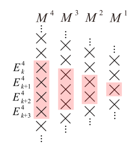
Figure 14: Schematic picture of the eigenvalues (denoted by crosses) of the sub matrices for 4-orbital system. From the Cauchy interlacing inequality, the eigenvalues of $M^{k-1}$ should exist between the eigenvalues of $M^{k}$. If the eigenvalues of $M^{4}$ have 4-fold degeneracy ($E=E^{4}_{k}=E^{4}_{k+1}=E^{4}_{k+2}=E^{4}_{k+3}$), one of the eigenvalues of $M^{1}$ should coincide with $E$. The shaded crosses have the same energy $E$. This indicates the zeros have the $4$-fold degeneracy.

References

- Abrikosov et al. (1975) A. A. Abrikosov, L. P. Gorkov, and I. E. Dzyaloshinski, Methods of Quantum Field Theory in Statistical Physics (Dover, New York) (1975).
- Fetter and Walecka (2012) Alexander L Fetter and John Dirk Walecka, Quantum theory of many-particle systems (Dover, New York) (2012).
- Dzyaloshinskii (2003) Igor Dzyaloshinskii, “Some consequences of the Luttinger theorem: The Luttinger surfaces in non-Fermi liquids and Mott insulators,” Phys. Rev. B 68, 085113 (2003).
- Stanescu et al. (2007) Tudor D. Stanescu, Philip Phillips, and Ting-Pong Choy, “Theory of the Luttinger surface in doped Mott insulators,” Phys. Rev. B 75, 104503 (2007).
- Seki and Yunoki (2017) Kazuhiro Seki and Seiji Yunoki, “Topological interpretation of the Luttinger theorem,” Phys. Rev. B 96, 085124 (2017).
- Stanescu and Kotliar (2006) Tudor D. Stanescu and Gabriel Kotliar, “Fermi arcs and hidden zeros of the Green function in the pseudogap state,” Phys. Rev. B 74, 125110 (2006).
- Dave et al. (2013) Kiaran B. Dave, Philip W. Phillips, and Charles L. Kane, “Absence of Luttinger’s Theorem due to Zeros in the Single-Particle Green Function,” Phys. Rev. Lett. 110, 090403 (2013).
- Sakai et al. (2010) Shiro Sakai, Yukitoshi Motome, and Masatoshi Imada, “Doped high- cuprate superconductors elucidated in the light of zeros and poles of the electronic Green’s function,” Phys. Rev. B 82, 134505 (2010).
- Yamaji and Imada (2011) Youhei Yamaji and Masatoshi Imada, “Composite fermion theory for pseudogap phenomena and superconductivity in underdoped cuprate superconductors,” Phys. Rev. B 83, 214522 (2011).
- Kane and Mele (2005) C. L. Kane and E. J. Mele, “ Topological Order and the Quantum Spin Hall Effect,” Phys. Rev. Lett. 95, 146802 (2005).
- Hasan and Kane (2010) M. Z. Hasan and C. L. Kane, “Colloquium: Topological insulators,” Rev. Mod. Phys. 82, 3045–3067 (2010).
- Qi and Zhang (2011) Xiao-Liang Qi and Shou-Cheng Zhang, “Topological insulators and superconductors,” Rev. Mod. Phys. 83, 1057–1110 (2011).
- Ando (2013) Yoichi Ando, “Topological insulator materials,” Journal of the Physical Society of Japan 82, 102001 (2013).
- Chiu et al. (2016) Ching-Kai Chiu, Jeffrey C. Y. Teo, Andreas P. Schnyder, and Shinsei Ryu, “Classification of topological quantum matter with symmetries,” Rev. Mod. Phys. 88, 035005 (2016).
- Ryu et al. (2010) Shinsei Ryu, Andreas P Schnyder, Akira Furusaki, and Andreas W W Ludwig, “Topological insulators and superconductors: tenfold way and dimensional hierarchy,” New Journal of Physics 12, 065010 (2010).
- Kitaev (2009) Alexei Kitaev, “Periodic table for topological insulators and superconductors,” in AIP conference proceedings, Vol. 1134 (American Institute of Physics, 2009) pp. 22–30.
- Essin and Gurarie (2011) Andrew M. Essin and Victor Gurarie, “Bulk-boundary correspondence of topological insulators from their respective Green’s functions,” Phys. Rev. B 84, 125132 (2011).
- Fu and Kane (2007) Liang Fu and C. L. Kane, “Topological insulators with inversion symmetry,” Phys. Rev. B 76, 045302 (2007).
- Kruthoff et al. (2017) Jorrit Kruthoff, Jan de Boer, Jasper van Wezel, Charles L. Kane, and Robert-Jan Slager, “Topological Classification of Crystalline Insulators through Band Structure Combinatorics,” Phys. Rev. X 7, 041069 (2017).
- Po et al. (2017) Hoi Chun Po, Ashvin Vishwanath, and Haruki Watanabe, “Symmetry-based indicators of band topology in the 230 space groups,” Nature Communications 8, 1–9 (2017).
- Bradlyn et al. (2017) Barry Bradlyn, L Elcoro, Jennifer Cano, MG Vergniory, Zhijun Wang, C Felser, MI Aroyo, and B Andrei Bernevig, “Topological quantum chemistry,” Nature 547, 298–305 (2017).
- Tang et al. (2019a) Feng Tang, Hoi Chun Po, Ashvin Vishwanath, and Xiangang Wan, “Efficient topological materials discovery using symmetry indicators,” Nature Physics 15, 470–476 (2019a).
- Zhang et al. (2019) Tiantian Zhang, Yi Jiang, Zhida Song, He Huang, Yuqing He, Zhong Fang, Hongming Weng, and Chen Fang, “Catalogue of topological electronic materials,” Nature 566, 475–479 (2019).
- Tang et al. (2019b) Feng Tang, Hoi Chun Po, Ashvin Vishwanath, and Xiangang Wan, “Comprehensive search for topological materials using symmetry indicators,” Nature 566, 486–489 (2019b).
- Vergniory et al. (2019) MG Vergniory, L Elcoro, Claudia Felser, Nicolas Regnault, B Andrei Bernevig, and Zhijun Wang, “A complete catalogue of high-quality topological materials,” Nature 566, 480–485 (2019).
- Tang et al. (2019c) Feng Tang, Hoi Chun Po, Ashvin Vishwanath, and Xiangang Wan, “Topological materials discovery by large-order symmetry indicators,” Science Advances 5, eaau8725 (2019c).
- Xu et al. (2020) Yuanfeng Xu, Luis Elcoro, Zhi-Da Song, Benjamin J Wieder, MG Vergniory, Nicolas Regnault, Yulin Chen, Claudia Felser, and B Andrei Bernevig, “High-throughput calculations of magnetic topological materials,” Nature 586, 702–707 (2020).
- Iraola et al. (2021) Mikel Iraola, Niclas Heinsdorf, Apoorv Tiwari, Dominik Lessnich, Thomas Mertz, Francesco Ferrari, Mark H. Fischer, Stephen M. Winter, Frank Pollmann, Titus Neupert, Roser Valentí, and Maia G. Vergniory, “Towards a topological quantum chemistry description of correlated systems: The case of the Hubbard diamond chain,” Phys. Rev. B 104, 195125 (2021).
- Denton et al. (2022) Peter Denton, Stephen Parke, Terence Tao, and Xining Zhang, “Eigenvectors from eigenvalues: a survey of a basic identity in linear algebra,” Bulletin of the American Mathematical Society 59, 31–58 (2022).
- Gurarie (2011) V. Gurarie, “Single-particle Green’s functions and interacting topological insulators,” Phys. Rev. B 83, 085426 (2011).
- Wang and Zhang (2012) Zhong Wang and Shou-Cheng Zhang, “Simplified Topological Invariants for Interacting Insulators,” Phys. Rev. X 2, 031008 (2012).
- Wang and Yan (2013) Zhong Wang and Binghai Yan, “Topological Hamiltonian as an exact tool for topological invariants,” Journal of Physics: Condensed Matter 25, 155601 (2013).
- González and Fernández-Rossier (2012) J. W. González and J. Fernández-Rossier, “Impurity states in the quantum spin Hall phase in graphene,” Phys. Rev. B 86, 115327 (2012).
- Slager et al. (2015) Robert-Jan Slager, Louk Rademaker, Jan Zaanen, and Leon Balents, “Impurity-bound states and Green’s function zeros as local signatures of topology,” Phys. Rev. B 92, 085126 (2015).
- Alvarado et al. (2020) M. Alvarado, A. Iks, A. Zazunov, R. Egger, and A. Levy Yeyati, “Boundary Green’s function approach for spinful single-channel and multichannel Majorana nanowires,” Phys. Rev. B 101, 094511 (2020).
- Benalcazar et al. (2017) Wladimir A Benalcazar, B Andrei Bernevig, and Taylor L Hughes, “Quantized electric multipole insulators,” Science 357, 61–66 (2017).
- Schindler et al. (2018) Frank Schindler, Ashley M Cook, Maia G Vergniory, Zhijun Wang, Stuart SP Parkin, B Andrei Bernevig, and Titus Neupert, “Higher-order topological insulators,” Science Advances 4, eaat0346 (2018).
- Wilkinson (1963) J. H. Wilkinson, Rounding errors in algebraic processes. Prentice-Hall, Inc., Engle-wood Cliffs, N.J. (1963).
- Hwang (2004) Suk-Geun Hwang, “Cauchy’s interlace theorem for eigenvalues of Hermitian matrices,” The American Mathematical Monthly 111, 157–159 (2004).
- Kohmoto (1985) Mahito Kohmoto, “Topological invariant and the quantization of the Hall conductance,” Annals of Physics 160, 343–354 (1985).
- Haldane (1988) F. D. M. Haldane, “Model for a Quantum Hall Effect without Landau Levels: Condensed-Matter Realization of the ”Parity Anomaly”,” Phys. Rev. Lett. 61, 2015–2018 (1988).
- Qi et al. (2008) Xiao-Liang Qi, Taylor L. Hughes, and Shou-Cheng Zhang, “Topological field theory of time-reversal invariant insulators,” Phys. Rev. B 78, 195424 (2008).
- Liu et al. (2010) Chao-Xing Liu, Xiao-Liang Qi, HaiJun Zhang, Xi Dai, Zhong Fang, and Shou-Cheng Zhang, “Model Hamiltonian for topological insulators,” Phys. Rev. B 82, 045122 (2010).
- Su et al. (1979) W. P. Su, J. R. Schrieffer, and A. J. Heeger, “Solitons in Polyacetylene,” Phys. Rev. Lett. 42, 1698–1701 (1979).
- Velasco and Paredes (2017) Carlos G. Velasco and Belén Paredes, “Realizing and Detecting a Topological Insulator in the AIII Symmetry Class,” Phys. Rev. Lett. 119, 115301 (2017).
- Liu et al. (2019) Zhu-Xi Liu, Zhi-Hua Li, and An-Min Wang, “Fractional charged edge states in ladder topological insulators,” Journal of Physics: Condensed Matter 31, 125402 (2019).
- Fu et al. (2007) Liang Fu, C. L. Kane, and E. J. Mele, “Topological Insulators in Three Dimensions,” Phys. Rev. Lett. 98, 106803 (2007).
- Turner et al. (2010) Ari M. Turner, Yi Zhang, and Ashvin Vishwanath, “Entanglement and inversion symmetry in topological insulators,” Phys. Rev. B 82, 241102(R) (2010).
- Matsugatani and Watanabe (2018) Akishi Matsugatani and Haruki Watanabe, “Connecting higher-order topological insulators to lower-dimensional topological insulators,” Phys. Rev. B 98, 205129 (2018).
- Fang and Fu (2019) Chen Fang and Liang Fu, “New classes of topological crystalline insulators having surface rotation anomaly,” Science Advances 5, eaat2374 (2019).
- (51) http://www.physics.rutgers.edu/pythtb/.
- Fukui (2020) Takahiro Fukui, “Theory of edge states based on the Hermiticity of tight-binding Hamiltonian operators,” Phys. Rev. Research 2, 043136 (2020).
- Hatsugai (1993) Yasuhiro Hatsugai, “Edge states in the integer quantum Hall effect and the Riemann surface of the Bloch function,” Phys. Rev. B 48, 11851–11862 (1993).
- Shindou and Nagaosa (2001) Ryuichi Shindou and Naoto Nagaosa, “Orbital Ferromagnetism and Anomalous Hall Effect in Antiferromagnets on the Distorted fcc Lattice,” Phys. Rev. Lett. 87, 116801 (2001).
- Murakami (2007) Shuichi Murakami, “Phase transition between the quantum spin Hall and insulator phases in 3D: emergence of a topological gapless phase,” New Journal of Physics 9, 356 (2007).
- Wan et al. (2011) Xiangang Wan, Ari M. Turner, Ashvin Vishwanath, and Sergey Y. Savrasov, “Topological semimetal and Fermi-arc surface states in the electronic structure of pyrochlore iridates,” Phys. Rev. B 83, 205101 (2011).
- Burkov (2018) AA Burkov, “Weyl metals,” Ann. Rev. Cond. Mat. Phys. 9, 359–378 (2018).
- Wang et al. (2012a) Zhijun Wang, Yan Sun, Xing-Qiu Chen, Cesare Franchini, Gang Xu, Hongming Weng, Xi Dai, and Zhong Fang, “Dirac semimetal and topological phase transitions in Bi (, K, Rb),” Phys. Rev. B 85, 195320 (2012a).
- Morimoto and Furusaki (2014) Takahiro Morimoto and Akira Furusaki, “Weyl and Dirac semimetals with topological charge,” Phys. Rev. B 89, 235127 (2014).
- Yang and Nagaosa (2014) Bohm-Jung Yang and Naoto Nagaosa, “Classification of stable three-dimensional Dirac semimetals with nontrivial topology,” Nature Communications 5, 4898 (2014).
- Rice and Mele (1982) M. J. Rice and E. J. Mele, “Elementary Excitations of a Linearly Conjugated Diatomic Polymer,” Phys. Rev. Lett. 49, 1455–1459 (1982).
- Xiao et al. (2010) Di Xiao, Ming-Che Chang, and Qian Niu, “Berry phase effects on electronic properties,” Rev. Mod. Phys. 82, 1959–2007 (2010).
- Wang et al. (2021) Tong Wang, Zhiming Pan, Tomi Ohtsuki, Ilya A. Gruzberg, and Ryuichi Shindou, “Multicriticality of two-dimensional class-D disordered topological superconductors,” Phys. Rev. B 104, 184201 (2021).
- Li et al. (2009) Jian Li, Rui-Lin Chu, J. K. Jain, and Shun-Qing Shen, “Topological Anderson Insulator,” Phys. Rev. Lett. 102, 136806 (2009).
- Kobayashi et al. (2013) Koji Kobayashi, Tomi Ohtsuki, and Ken-Ichiro Imura, “Disordered Weak and Strong Topological Insulators,” Phys. Rev. Lett. 110, 236803 (2013).
- Wang et al. (2012b) Lei Wang, Hua Jiang, Xi Dai, and X. C. Xie, “Pole expansion of self-energy and interaction effect for topological insulators,” Phys. Rev. B 85, 235135 (2012b).
- Witczak-Krempa et al. (2014) William Witczak-Krempa, Gang Chen, Yong Baek Kim, and Leon Balents, “Correlated Quantum Phenomena in the Strong Spin-Orbit Regime,” Annual Review of Condensed Matter Physics 5, 57–82 (2014).
- Tran et al. (2022) Minh-Tien Tran, Duong-Bo Nguyen, Hong-Son Nguyen, and Thanh-Mai Thi Tran, “Topological Green function of interacting systems,” Phys. Rev. B 105, 155112 (2022).
- Hatsugai (2004) Yasuhiro Hatsugai, “Explicit Gauge Fixing for Degenerate Multiplets: A Generic Setup for Topological Orders,” J. Phys. Soc. Jpn. 73, 2604–2607 (2004).
- Fukui and Hatsugai (2007) Takahiro Fukui and Yasuhiro Hatsugai, “Quantum Spin Hall Effect in Three Dimensional Materials: Lattice Computation of Z2 Topological Invariants and Its Application to Bi and Sb,” J. Phys. Soc. Jpn. 76, 053702 (2007).
- Chen (2019) Xiaomei Chen, “Note on eigenvectors from eigenvalues,” arXiv:1911.09081 (2019).
- Price (2020) Hannah M. Price, “Four-dimensional topological lattices through connectivity,” Phys. Rev. B 101, 205141 (2020).
- Wang et al. (2020) You Wang, Hannah M Price, Baile Zhang, and YD Chong, “Circuit implementation of a four-dimensional topological insulator,” Nature Communications 11, 1–7 (2020).