Bayesian Poroelastic Aquifer Characterization from
InSAR Surface Deformation Data
Part II: Quantifying the Uncertainty

Abstract

Uncertainty quantification of groundwater (GW) aquifer parameters is critical for efficient management and sustainable extraction of GW resources. These uncertainties are introduced by the data, model, and prior information on the parameters. Here we develop a Bayesian inversion framework that uses Interferometric Synthetic Aperture Radar (InSAR) surface deformation data to infer the laterally heterogeneous permeability of a transient linear poroelastic model of a confined GW aquifer. The Bayesian solution of this inverse problem takes the form of a posterior probability density of the permeability. Exploring this posterior using classical Markov chain Monte Carlo (MCMC) methods is computationally prohibitive due to the large dimension of the discretized permeability field and the expense of solving the poroelastic forward problem. However, in many partial differential equation (PDE)-based Bayesian inversion problems, the data are only informative in a few directions in parameter space. For the poroelasticity problem, we prove this property theoretically for a one-dimensional problem and demonstrate it numerically for a three-dimensional aquifer model. We design a generalized preconditioned Crank–Nicolson (gpCN) MCMC method that exploits this intrinsic low dimensionality by using a low-rank based Laplace approximation of the posterior as a proposal, which we build scalably. The feasibility of our approach is demonstrated through a real GW aquifer test in Nevada. The inherently two dimensional nature of InSAR surface deformation data informs a sufficient number of modes of the permeability field to allow detection of major structures within the aquifer, significantly reducing the uncertainty in the pressure and the displacement quantities of interest.

Water Resources Research

University of Texas at Austin, Oden Institute for Computational Engineering and Sciences, Austin, TX, United States University of Texas at Austin, Geological Sciences, Austin, TX, United States University of Texas at Austin, Aerospace Engineering & Engineering Mechanics, Austin, TX, United States Washington University in St. Louis, Electrical and Systems Engineering, St. Louis, MO, United States University of Texas at Austin, Mechanical Engineering, Austin, TX, United States

Amal Alghamdiamal.m.alghamdi@gmail.com

Using InSAR data reduces the uncertainty in selected quantities of interest compared to using prior knowledge only

The preconditioned Crank–Nicolson (pCN) MCMC method is extended to exploit posterior curvature and allow better chain mixing

We demonstrate the intrinsic low dimensionality of the poroelastic inverse problem that is critical for the success of the MCMC method

1 Introduction

Efficient groundwater (GW) resources management is critical for mitigating the global-scale problem of GW depletion [Wada . (2010), Wada . (2012), Wada . (2014), Famiglietti (2014)]. This is the result of extracting GW at rates that exceed the natural recharge, which then leads to significant drops in GW pressure and (possibly irreversible) compaction [Wada . (2010), Konikow  Kendy (2005), Xue . (2005), Holzer  Galloway (2005)]. Making informed management and control decisions requires accurate GW aquifer models, typically in the form of a time-dependent partial differential equation (PDE). These models are used to predict the aquifer response (e.g. GW pressure drop and aquifer compaction) to GW extraction activities. The major source of uncertainty in these models is the uncertainty in the aquifer properties [Eaton (2006), Bohling  Butler (2010), Oliver  Chen (2011)]. The goal of our work is to devise a framework to systematically quantify the uncertainty in GW aquifer model properties. Here we only consider uncertainty in one parameter field, the aquifer permeability, and one data source, surface deformation data, but the framework we present can be generalized to multiple parameter fields and data sources. To estimate the permeability, we take advantage, in particular, of the evergrowing InSAR data that provide frequent, large-scale, and up to sub-millimeter accurate surface deformation measurements globally [Ferretti . (2007), Tomás . (2014)].

Bayes’ theorem—which has been adopted in GW applications since as early as 1986 [Carrera  Neuman (19861), Carrera  Neuman (19862), Carrera  Neuman (19863), McLaughlin  Townley (1996), Linde . (2017)]—provides a natural means of incorporating observational data, e.g., pressure or surface deformation data at the aquifer site, to quantify the uncertainty in the aquifer model parameters (such as physical properties, source terms, and/or boundary or initial conditions). The Bayesian framework updates our assumed “prior” knowledge about the aquifer parameters through what is known as the “likelihood” distribution, which determines how likely it is for the observational data to result from the modeled system with a particular parameter realization. The updated probability distribution is called the “posterior” distribution and is regarded as the solution of the inverse problem. Bayesian inversion, therefore, provides a characterization of the uncertainty in the parameters, as opposed to finding just a point estimate as is with deterministic inversion.

The Markov chain Monte Carlo (MCMC) method is often the method of choice for characterizing the posterior distribution for PDE-based Bayesian inverse problems. MCMC generates samples of the posterior probability density function (PDF)—each of which requires solution of at least the forward PDEs—from which sample statistics can be computed. Conventional MCMC methods view the parameter-to-observable map as a black box and thus are not capable of exploiting the structure of this map to accelerate convergence of MCMC chains. As such, most work on Bayesian inversion governed by PDEs has been restricted to simple PDEs or low parameter dimensions (or both).

Over the past decade, several powerful MCMC methods have emerged that exploit the geometry and smoothness—and in some cases the underlying low-dimensionality—of the parameter-to-observable map to enable efficient MCMC sampling from high-dimensional PDE-based posteriors [Cui . (2016), Flath . (2011), Martin . (2012), Bui-Thanh . (2013), Petra . (2014), Beskos . (2017)]. These methods have been applied to several large-scale Bayesian inverse problems governed by complex forward problems, including seismic wave propagation [Martin . (2012)] and ice sheet flow [Isaac . (2015)]. What these methods all have in common is the use of the Hessian of the negative log posterior to exploit the geometry of the posterior. Moreover, the low rank structure of the Hessian can be used to identify the (often) low dimensional manifold (of dimension $r$ much smaller than the nominal dimension of the discretized parameters) on which the parameters are informed by the data. To that end, randomized methods (e.g., randomized singular value decomposition and randomized generalized eigensolvers) are devised to identify this low dimensional manifold at a cost of $O(r)$ PDE solves only. Characterizing high-dimensional posterior distributions governed by three-dimensional transient poroelastic GW aquifer models has been explored by HesseStadler14 via a Gaussian approximation of the posterior distribution for model problems. Full MCMC sampling of posteriors governed by high-dimensional GW models of such complexity has yet to be explored.

In AlghamdiHesseChenEtAl2020A, Part I of this two-part series of articles, we built a Bayesian framework to characterize the lateral heterogeneity in a three-dimensional time-dependent poroelastic aquifer model and applied it to a test case in Nevada using InSAR surface deformation data. There, we addressed the choice of the prior distribution and the data noise model. We also took a first step in exploring the posterior by inverting for the maximum a posteriori (MAP) point, which is the most likely permeability realization with respect to the posterior distribution. We used independent GPS measurements [Burbey . (2006)] for validation. A brief summary of the pertinent results from Part I is provided in section 3.

We summarize the contribution of Part II as follows: (1) We demonstrate the decaying eigenvalues of the data misfit part of the Hessian analytically, through Fourier analysis, for a simplified 1D poroelasticity problem. We additionally provide numerical evidence of the data misfit Hessian compactness for the three-dimensional fully-coupled quasi-static linear poroelastic aquifer model considered here. This property determines the applicability of the aforementioned class of scalable MCMC methods. (2) We propose a generalization of the preconditioned Crank–Nicolson (pCN) MCMC method [Cotter . (2012)], referred to as gpCN thereafter, that identifies and exploits this low dimensional manifold using randomized eigensolvers to construct a low-rank based Laplace approximation of the posterior. Besides the initial cost of creating the low-rank based Laplace approximation, which is negligible in comparison to the cost of generating MCMC chains, gpCN has no additional cost per MCMC sample in comparison to pCN. Furthermore, we compare convergence properties of pCN and gpCN. (3) We apply gpCN to characterize the high-dimensional subsurface permeability for the Nevada test case aquifer, and quantify the associated uncertainty (both in the parameters and the selected state-variable-based quantities of interest (QoIs)). We discuss how information from the data reduces the prior uncertainty in the parameters and the state variables in terms of the location in the physical domain and the dominant parameters modes inferred from the data. The three integrated contributions demonstrate a successful design and application of a scalable MCMC method to a real-world GW Bayesian inverse problem governed by a coupled forward problem with high dimensional parameters and using InSAR data.

The reminder of the paper is structured as follows. In section 2, we review the quasi-static linear poroelasticity model and the Bayesian framework that we established in Part I. We discuss low-rank based Laplace approximation of the posterior and present gpCN, our generalization of pCN MCMC method. We describe the test case to which we apply our framework in section 3. We demonstrate gpCN performance and present results on characterizing the uncertainty in the permeability and selected state-variable-based QoI for the Nevada test case in section 4. We summarize our conclusions in section 5.

2 Methods

In Part I of this two-part series of articles, we formulate a Bayesian inversion framework governed by quasi-static linear poroelasticity. The solution of the Bayesian inverse problem takes the form of a posterior distribution that characterizes the heterogeneity of groundwater aquifer permeability. Here, we review the forward model, the quasi-static linear poroelasticity model, and the formulation of the inverse problem, the Bayesian framework, in sections 2.1 and 2.2, respectively. We also demonstrate the compactness of the data misfit Hessian for a simplified one dimensional poroelasticity problem. In sections 2.3 and 2.4, we build a low-rank based Laplace approximation and present the gpCN MCMC method that exploits this intrinsic low dimensionality in the poroelasticity inverse problem.

2.1 Quasi-Static Linear Poroelasticity

In the Bayesian inversion framework, we model the aquifer as a poroelastic medium governed by the linear poroelasticity theory developed by Biot1941. Biot theory describes the coupling between the fluid pressure field in a saturated porous medium and the accompanying elastic deformation of the solid skeleton. The classical formulation of Biot system in a space-time domain $\Omega\times(0,T]$ can be written as

$$\left(S_{\epsilon}p+\alpha\nabla\cdot\mathbf{u}\right)_{t}-\nabla\cdot\left(\frac{\kappa}{\mu}\nabla p\right)= f_{p}$$

$$-\nabla\cdot\left(\boldsymbol{\sigma}(\mathbf{u})-\alpha p\mathbf{I}\right)= \mathbf{f_{u}},$$ (1)

where $(\cdot)_{t}$ denotes time derivative, $p=p(\mathbf{x},t)$ is the deviation from hydrostatic pressure, $\mathbf{u}=\mathbf{u}(\mathbf{x},t)$ is the displacement of the solid skeleton, $f_{p}=f_{p}(\mathbf{x},t)$ is a fluid source per unit volume, $\mathbf{f_{u}}=\mathbf{f_{u}}(\mathbf{x},t)$ is the body force per unit volume, $S_{\epsilon}$ is the specific storage, $\kappa(\mathbf{x})$ is the medium permeability field, $\mu$ is the dynamic viscosity of the pore fluid, and $\alpha$ is the Biot–Willis coupling parameter. The tensor $\boldsymbol{\sigma}(\mathbf{u})$ is the stress tensor for isotropic linear elasticity, and it is parameterized by the drained shear modulus $G$ and the Poisson’s ratio $\nu$. We write the unknown medium permeability $\kappa(\mathbf{x})$ in terms of the log-permeability field, which we denote $m(\mathbf{x})$, so that $\kappa(\mathbf{x})=e^{m(\mathbf{x})}$. This parameterization ensures that the inferred permeability field is positive when solving the inverse problem for $m(\mathbf{x})$. The system (1) together with well-defined boundary and initial conditions, given in AlghamdiHesseChenEtAl2020A, form the forward problem.

We use a three-field formulation of the poroelasticity system (1) in which Darcy flux is introduced as a state variable $\mathbf{q}(\mathbf{x},t)=-\frac{\kappa}{\mu}\nabla p$, adding a third equation to the system (1). Following FerronatoCastellettoGambolati10, we employ a mixed finite element method (MFEM) to discretize the three-field formulation in space and use backward Euler method for discretization in time. In this MFEM, the pressure $p$ is approximated by piecewise constant functions, the displacement $\mathbf{u}$ is approximated in the first-order Lagrange polynomial space, and the flux $\mathbf{q}$ is approximated in the lowest-order Raviart–Thomas space. This MFEM discretization has the advantage of conserving mass discretely and reducing the non-physical pressure oscillations that can form in some other discretizations of the poroelasticity system [Phillips  Wheeler (2009), Ferronato . (2010), Haga . (2012)]. To simplify notation, we define the discretized “global” space-time system, which combines solving for all time steps simultaneously, as

$$\mathbf{\bar{S}}(\mathbf{m})\mathbf{\bar{X}}=\mathbf{\bar{F}},$$ (2)

where the block lower triangular matrix $\mathbf{\bar{S}}$ combines the discretized differential operators of the three-field formulation of the poroelasticity system (1). $\mathbf{\bar{S}}$ depends on the discretized log permeability $\mathbf{m}\in\mathbb{R}^{n_{n}}$, which we approximate in the first order Lagrange polynomial space, where $n_{n}$ is the number of degrees of freedom (DOFs) of the discretized parameter field. The vector $\mathbf{\bar{F}}$ combines the source terms and the natural boundary conditions at all time steps, and the vector $\mathbf{\bar{X}}$ consists of the pressure, displacement, and fluid flux DOFs at all time steps as well. The discretization details can be found in Part I [Alghamdi . (2020)].

2.2 Poroelasticity Bayesian Inversion Framework Constrained by InSAR Surface Deformation Data

Our goal is to characterize the aquifer heterogeneous permeability $\kappa=e^{m}$ in the poroelasticity model (1) from InSAR Line-of-Sight (LOS) surface deformation data $\mathbf{d}^{\text{obs}}\in\mathbb{R}^{n_{\text{obs}}}$, where $n_{\text{obs}}$ is the number of observational data (total number of pixels in deformation maps in this case). The LOS surface deformation $u_{\text{LOS}}$ is given by

$$u_{\text{LOS}}=\alpha_{1}u_{1}+\alpha_{2}u_{2}+\alpha_{3}u_{3},$$ (3)

where $u_{1}$, $u_{2}$ and $u_{3}$ are the east, north and vertical surface displacements, respectively, and $\alpha_{1}$, $\alpha_{2}$ and $\alpha_{3}$ are the eastward, northward and vertical components of the LOS unit look vector $\alpha_{\text{LOS}}=[\alpha_{1},\alpha_{2},\alpha_{3}]$. In this study, we only use one LOS net deformation map available at $t=t_{\text{InSAR}}$. In general, multiple deformation maps or deformation time series can be available.

Assuming modeling errors are negligible compared to noise in the data, for a given log permeability field $\mathbf{m}(\mathbf{x})$, the relation between the observational data $\mathbf{d}^{\text{obs}}$ and the model output is given by

$$\mathbf{d}^{\text{obs}}=\mathbfcal{F}(\mathbf{m})+\boldsymbol{\eta}.$$ (4)

The map $\mathbfcal{F}(\cdot):\mathbb{R}^{n_{n}}\rightarrow\mathbb{R}^{n_{\text{obs}}}$ is the parameter-to-observable map which, for a given $\mathbf{m}$, gives the observables, i.e the modeled LOS surface deformation values at the observational data locations (pixels centers) and times. Evaluating $\mathbfcal{F}(\mathbf{m})$ requires solving model (1) using the given log permeability $\mathbf{m}$. In particular, $\mathbfcal{F}(\mathbf{m})\coloneqq\mathbf{\bar{B}}\mathbf{\bar{X}}=\mathbf{\bar{B}}\mathbf{\bar{S}}(\mathbf{m})^{-1}\mathbf{\bar{F}}$, where we define the pointwise linear observation operator $\mathbf{\bar{B}}$ which extracts the pointwise observables from the modeled displacement DOFs included in the global vector $\mathbf{\bar{X}}$. The solution $\mathbf{\bar{X}}$ is obtained by solving the “global” system (2). The random vector $\boldsymbol{\eta}\sim\mathcal{N}(\mathbf{0},\mathbf{\Gamma}_{\text{noise}})$ is measurement noise which we assume is additive and Gaussian with mean $\mathbf{0}$ and covariance matrix $\mathbf{\Gamma}_{\text{noise}}\in\mathbb{R}^{n_{\text{obs}}\times n_{\text{obs}}}$.

We use relation (4) to define the likelihood probability distribution that determines how likely it is for the observational data $\mathbf{d}^{\text{obs}}$ to be measured from an aquifer with permeability $\mathbf{m}$—in the absence of model error. In other words, the likelihood distribution is the probability distribution of the discrepancy between the observed data and the model outcome which, based on the relation (4), is given by

$$\pi_{\text{likelihood}}(\mathbf{d}^{\text{obs}}|\mathbf{m})\propto e^{-\ell(\mathbf{d}^{\text{obs}};\mathbf{m})},$$ (5)

where the symbol $\propto$ denotes equality up to a multiplicative constant and $\ell$ is the negative log of the likelihood, or the data misfit, which is given by

$$\ell(\mathbf{d}^{\text{obs}};\mathbf{m})=\frac{1}{2}(\mathbfcal{F}(\mathbf{m})-\mathbf{d}^{\text{obs}})^{T}\mathbf{\Gamma}_{\text{noise}}^{-1}(\mathbfcal{F}(\mathbf{m})-\mathbf{d}^{\text{obs}}).$$ (6)

Bayes theory gives the posterior probability distribution $\pi_{\text{post}}(\mathbf{m}|\mathbf{d}^{\text{obs}})$, which quantifies the uncertainty in the parameter $\mathbf{m}$ given the observational data $\mathbf{d}^{\text{obs}}$. The posterior distribution incorporates information about the model and the data, via the likelihood distribution. Statistical prior assumptions about the parameters are encoded into the prior distribution $\pi_{\text{prior}}(\mathbf{m})$. Bayesian formulation of inverse problems was introduced in [Tarantola . (1982)] and is given by

$$\pi_{\text{post}}(\mathbf{m}|\mathbf{d}^{\text{obs}}) \propto\pi_{\text{likelihood}}(\mathbf{d}^{\text{obs}}|\mathbf{m})\pi_{\text{prior}}(\mathbf{m})$$

$$\propto\text{exp}\left(-\frac{1}{2}(\mathbf{\bar{B}}\mathbf{\bar{X}}-\mathbf{d}^{\text{obs}})^{T}\mathbf{\Gamma}_{\text{noise}}^{-1}(\mathbf{\bar{B}}\mathbf{\bar{X}}-\mathbf{d}^{\text{obs}})-\frac{1}{2}(\mathbf{m}-\bar{\mathbf{m}})^{T}\mathbf{\Gamma}_{\text{prior}}^{-1}(\mathbf{m}-\bar{\mathbf{m}})\right).$$ (7)

We assume the prior distribution is a discretized Matérn Gaussian field with mean $\bar{\mathbf{m}}\in\mathbb{R}^{n_{n}}$ and covariance matrix $\mathbf{\Gamma}_{\text{prior}}\in\mathbb{R}^{n_{n}\times n_{n}}$. The latter dictates our assumptions about the pointwise variance and the spatial correlation of the log permeability field features. For this class of priors, the precision operator $\mathbf{\Gamma}_{\text{prior}}^{-1}$ admits a representation $\mathbf{\Gamma}_{\text{prior}}^{-1}=\mathbf{A}\mathbf{M}_{m}^{-1}\mathbf{A}$ in terms of an elliptic differential operator $\mathbf{A}$ and a mass matrix $\mathbf{M}_{m}$ in the discretized parameter space [Lindgren . (2011), Alghamdi . (2020)].

The posterior distribution is a distribution in a very large dimensional space $\mathbb{R}^{n_{n}}$, and evaluating the posterior at a single realization $\mathbf{m}$ requires solving the model (1) forward in time. Computing moments and other expected values of interest from the posterior distribution is computationally prohibitive using traditional MCMC sampling methods. Fortunately, in many PDE-based Bayesian inversion problems, the data are informative in only relatively few directions in parameter space $r\ll n_{n}$. This property can be exploited to obtain low-rank based approximations of the posterior, which additionally can be used to build effective MCMC proposals, as we present in the remaining of this section.

2.3 Low-Rank Based Laplace Approximation of the Posterior

2.3.1 The Laplace Approximation

In Part I we focused on solution of the optimization problem of maximizing the posterior distribution to find the MAP point $\mathbf{m}_{\text{MAP}}$. Besides being the most likely realization of the permeability field, the MAP point is also needed to form the Laplace approximation of the posterior, which is a Gaussian approximation obtained by making a quadratic approximation of the negative log posterior at the MAP point [MacKay (2003)]. This approximation is valid if the parameter-to-observable map is approximately linear over the support of the prior distribution. Additionally, it can be used in building effective proposals for dimension invariant MCMC algorithms as we discuss in section 2.4.

The negative log of the posterior (7) can be written as

$$-\log \left(\pi_{\text{post}}\left(\mathbf{m}\right)\right)$$

$$= \frac{1}{2}\left(\mathbfcal{F}(\mathbf{m})-\mathbf{d}^{\text{obs}}\right)^{T}\mathbf{\Gamma}_{\text{noise}}^{-1}\left(\mathbfcal{F}(\mathbf{m})-\mathbf{d}^{\text{obs}}\right)+\frac{1}{2}\left(\mathbf{m}-\bar{\mathbf{m}}\right)^{T}\mathbf{\Gamma}_{\text{prior}}^{-1}\left(\mathbf{m}-\bar{\mathbf{m}}\right)-c_{1},$$ (8)

where $c_{1}$ is the log of the posterior normalization constant. Using a Taylor expansion at the point $\mathbf{m}_{\text{MAP}}$ in parameter space, a quadratic approximation of (8) is given by

$$-\log \left(\pi_{\text{post}}\left(\mathbf{m}_{\text{MAP}}+\hat{\mathbf{m}}\right)\right)\approx c_{2}+\frac{1}{2}{\hat{\mathbf{m}}}^{T}\mathbf{H}(\mathbf{m}_{\text{MAP}})\hat{\mathbf{m}},$$ (9)

where $\hat{\mathbf{m}}=\mathbf{m}-\mathbf{m}_{\text{MAP}}$. To obtain (9), we use the fact that the gradient of the negative log posterior with respect to the parameter $\mathbf{m}$ is zero at the MAP point. The constant $c_{2}$ is defined as

$$c_{2}= \frac{1}{2}\left(\mathbfcal{F}(\mathbf{m}_{\text{MAP}})-\mathbf{d}^{\text{obs}}\right)^{T}\mathbf{\Gamma}_{\text{noise}}^{-1}\left(\mathbfcal{F}(\mathbf{m}_{\text{MAP}})-\mathbf{d}^{\text{obs}}\right)$$

$$+ \frac{1}{2}\left(\mathbf{m}_{\text{MAP}}-\bar{\mathbf{m}}\right)^{T}\mathbf{\Gamma}_{\text{prior}}^{-1}\left(\mathbf{m}_{\text{MAP}}-\bar{\mathbf{m}}\right)-c_{1}.$$ (10)

The matrix $\mathbf{H}(\mathbf{m}_{\text{MAP}})\in\mathbb{R}^{n_{n}\times n_{n}}$ is the Hessian operator of the negative log of the posterior (7) evaluated at the MAP point and it is given by

$$\mathbf{H}(\mathbf{m})=\mathbf{H}_{\text{misfit}}(\mathbf{m})+\mathbf{\Gamma}_{\text{prior}}^{-1},$$ (11)

where the data misfit Hessian $\mathbf{H}_{\text{misfit}}(\mathbf{m})$ is given by

$$\mathbf{H}_{\text{misfit}}(\mathbf{m})=\nabla\mathbfcal{F}(\mathbf{m})^{T}\mathbf{\Gamma}_{\text{noise}}^{-1}\nabla\mathbfcal{F}(\mathbf{m})+\sum_{i}^{n_{\text{obs}}}{\left(\mathbf{\Gamma}_{\text{noise}}^{-1}(\mathbfcal{F}(\mathbf{m})-\mathbf{d}^{\text{obs}})\right)_{i}\nabla^{2}\mathbfcal{F}_{i}(\mathbf{m})}.$$ (12)

The resulting Laplace approximation is the Gaussian distribution:

$$\pi_{\text{Laplace}}(\mathbf{m})\sim \mathcal{N}\left(\mathbf{m}_{\text{MAP}},\mathbf{H}(\mathbf{m}_{\text{MAP}})^{-1}\right).$$ (13)

2.3.2 Spectral Properties of the Hessian

In many PDE-based inverse problems, it is often the case that the data misfit Hessian operator is compact and only a few parameter dimensions, $O(r)$, are informed by the data [Flath . (2011), Bui-Thanh . (2012), Isaac . (2015), Villa . (2020)]. In Alghamdi2020, we provide an analytical formula for the eigenvalues and the eigenfunctions of the Hessian of an idealized one-dimensional steady-state poroelasticity problem. We assume this problem is defined on an interval $[0,L]$, and that we have continuous deformation observations everywhere in this interval. Specifically, the eigenvalues $\lambda_{i}$ and eigenfunctions $\phi_{i}$ of the data misfit Hessian operator in this case are given by

$$\lambda_{i}=\frac{f_{L}^{2}\mu^{2}}{e^{2}\kappa_{0}^{4}}\left(\frac{2L}{i\pi}\right)^{4},\quad\phi_{i}(x)=\cos\left(\frac{i\pi x}{2L}\right),\quad i=1,3,5,...,$$ (14)

where $f_{L}$ is the Darcy flux at the boundary $x=L$, $e$ is Young’s modulus, and $\kappa_{0}$ is the constant permeability value at which the data misfit Hessian operator is evaluated. We note from the expressions in (14) that the eigenvalues have a rapid decay of $O(\frac{1}{i^{4}})$, and the eigenfunctions corresponding to dominant eigenvalues are smoother. This means that the more oscillatory a permeability mode is, the more difficult it is to infer from the deformation data. Note that the expected information gain (from prior to posterior) from the data in each mode is given by $\log(1+\lambda_{i})$ under a Gaussian assumption [Alexanderian . (2016)]. The rapid decay of eigenvalues in  (14) implies that the data inform the permeability field in a low dimensional manifold. Although this analysis is carried out for an idealized one-dimensional case, numerical evidence suggests rapid eigenvalue decay—independent of the discretization dimension—of the data misfit Hessian of the 3D poroelasticity problem we study; see section 4. Moreover, analogous to the 1D analysis result, larger eigenvalues correspond to smoother eigenvectors.

2.3.3 Sampling from the Laplace Approximation

The gpCN method described in the next section requires the ability to generate samples $\boldsymbol{\eta}_{\text{Laplace}}$ from the distribution $\pi_{\text{Laplace}}(\mathbf{m})$. To sample from this Gaussian distribution, $\mathbf{H}^{-\frac{1}{2}}$ is applied to a white noise vector. However, constructing the Hessian matrix explicitly and computing its Cholesky factorization is computationally prohibitive in high parameter dimensions. The Hessian construction costs $n_{n}$ pairs of incremental forward (27) and incremental adjoint (28) poroelasticity solves; see A for details.

Instead of building the Hessian explicitly, we take advantage of the fact that applying the Hessian to a vector can be carried out in a matrix-free manner and costs only a pair of incremental forward and incremental adjoint solves, and the data misfit Hessian is inherently low-rank. This allows us to build a low-rank based representation of the Hessian at $\mathbf{m}_{\text{MAP}}$ by solving a generalized eigenvalue problem using a randomized generalized eigensolver—at a cost of just $O(r)$ incremental forward and adjoint poroelasticity solves. We use this approximation to create a low-rank based Laplace approximation, $\pi_{\text{Laplace,r}}(\mathbf{m})$, of the posterior.

The following approach of approximating the Hessian at the MAP point has been applied to the inverse problem for the basal friction coefficient of the Antarctic ice sheet [Isaac . (2015)], and is integrated in the hIPPYlib library [Villa . (2018)]. This approach is based on solving the generalized eigenvalue problem:

$$\mathbf{H}_{\text{misfit}}(\mathbf{m}_{\text{MAP}})\mathbf{w}_{i}=\lambda_{i}\mathbf{\Gamma}_{\text{prior}}^{-1}\mathbf{w}_{i}\quad\text{for}\quad i=1,..,r.$$ (15)

The eigenvalues $\lambda_{i}$ of this generalized eigenvalue problem indicate whether the corresponding eigendirection $\mathbf{w}_{i}$ in the high dimensional parameter space $\mathbb{R}^{n_{n}}$ is mostly informed by the data (when $\lambda_{i}>1$) or by the prior (when $\lambda_{i}<1$). Also, the magnitude of $\lambda_{i}$ reflects the level of certainty of inferring the corresponding eigendirection from the data. The diagonal matrix of the first $r$ dominant eigenvalues, $\lambda_{i}$, and the matrix of the corresponding eigenvectors, $\mathbf{w}_{i}$, of this generalized eigenvalue problem are denoted as $\mathbf{\Lambda}_{r}=\text{diag}([\lambda_{1},\lambda_{2},...,\lambda_{r}])$ and $\mathbf{W}_{r}=[\mathbf{w}_{1},..,\mathbf{w}_{r}]$, respectively. The matrix $\mathbf{W}_{r}$ has $\mathbf{\Gamma}_{\text{prior}}^{-1}$-orthonormal columns, that is $\mathbf{W}_{r}^{T}\mathbf{\Gamma}_{\text{prior}}^{-1}\mathbf{W}_{r}=\mathbf{I}_{r}$, where $\mathbf{I}_{r}$ denotes the identity matrix in $\mathbb{R}^{r}$.

The eigenvalue problem (15) along with the Sherman–Woodbury formula are then used to obtain the following low-rank approximation of the Laplace approximation covariance matrix (the inverse of the Hessian at the MAP point); see [Villa . (2020)]:

$$\mathbf{H}(\mathbf{m}_{\text{MAP}})^{-1} =(\mathbf{H}_{\text{misfit}}(\mathbf{m}_{\text{MAP}})+\mathbf{\Gamma}_{\text{prior}}^{-1})^{-1}$$

$$\approx\mathbf{\Gamma}_{\text{prior}}-\mathbf{W}_{r}\mathbf{D}_{r}\mathbf{W}_{r}^{T}.$$ (16)

The matrix $\mathbf{D}_{r}$ is given by $\mathbf{D}_{r}=\text{diag}([\frac{\lambda_{1}}{1+\lambda_{1}},\frac{\lambda_{2}}{1+\lambda_{2}},...,\frac{\lambda_{r}}{1+\lambda_{r}}])$. The value $\frac{\lambda_{i}}{1+\lambda_{i}}$ is negligible for $\lambda_{i}\ll 1$, which provides a basis for truncation. We denote the low-rank based covariance matrix given by the inverse of the Hessian in (16) by $\mathbf{\Gamma}_{\text{Laplace,r}}\coloneqq\mathbf{\Gamma}_{\text{prior}}-\mathbf{W}_{r}\mathbf{D}_{r}\mathbf{W}_{r}^{T}$. A sample $\boldsymbol{\eta}_{\text{Laplace,r}}$ from this low-rank based Laplace approximation $\pi_{\text{Laplace,r}}(\mathbf{m})=\mathcal{N}(\mathbf{m}_{\text{MAP}},\mathbf{\Gamma}_{\text{Laplace,r}})$ can be generated scalably using [Villa . (2020)]:

$$\boldsymbol{\eta}_{\text{Laplace,r}}=(\mathbf{I}-\mathbf{W}_{r}\mathbf{S}_{r}\mathbf{W}_{r}^{T}\mathbf{\Gamma}_{\text{prior}}^{-1})\boldsymbol{\eta}+\mathbf{m}_{\text{MAP}}$$ (17)

where $\mathbf{S}_{r}=\text{diag}([1-\frac{1}{\sqrt{1+\lambda_{1}}},1-\frac{1}{\sqrt{1+\lambda_{2}}},...,1-\frac{1}{\sqrt{1+\lambda_{r}}}])$ and $\boldsymbol{\eta}\sim\mathcal{N}(0,\mathbf{\Gamma}_{\text{prior}})$. The cost of sampling from this approximation is dominated by the cost of generating the prior sample $\boldsymbol{\eta}$ (mainly applying $\mathbf{A}^{-1}$ via a scalable multigrid solve as discussed in Part I), and the matrix–vector multiplications by sparse and low-rank matrices.

2.4 Generalized Preconditioned Crank-Nicolson (gpCN) MCMC method

To characterize the posterior distribution, MCMC methods generate samples of the posterior PDF (each of which requires at least a forward PDE solve) from which sample statistics can be computed. As stated earlier, for PDE-governed posteriors in a high dimensional parameter space, it is often the case that the low rank structure of the Hessian can be used to identify the low dimensional manifold on which the parameters are informed by the data, which limits the expensive PDE solves to exploration of just a low dimensional subspace of the parameter space.

In this work, we design a generalization of the preconditioned Crank–Nicolson (gpCN) MCMC method. Preconditioned Crank–Nicolson (pCN) is a dimension-invariant MCMC method that uses prior information to build the proposal distribution [Cotter . (2012), Pinski . (2015)]. The gpCN algorithm is also dimension-invariant, yet has the advantage of capturing posterior curvature information in a relatively inexpensive manner. It uses an approximation of the gradient and the low-rank based approximation of the Hessian at the MAP point discussed in section 2.3, rather than computing exact gradient directions and Hessian matrices at numerous samples in parameter space. The gpCN proposed sample $\boldsymbol{\eta}_{\text{prop}}^{(k)}$ in the ${k}^{\text{th}}$ Metropolis Hastings (MH) iteration (described in Algorithm 1) is given by

$$\boldsymbol{\eta}_{\text{prop}}^{(k)} =\mathbf{m}_{\text{MAP}}+\sqrt{1-\beta^{2}}(\boldsymbol{\eta}_{\text{post}}^{(k-1)}-\mathbf{m}_{\text{MAP}})+\beta\boldsymbol{\eta}_{0}^{(k)}$$ (18)

where $\boldsymbol{\eta}_{0}^{(k)}\sim\mathcal{N}(0,\mathbf{\Gamma}_{\text{Laplace,r}})$ and $\boldsymbol{\eta}_{\text{post}}^{(k-1)}$ is the ${(k-1)}^{\text{th}}$ MH iteration posterior sample. The proposed sample $\boldsymbol{\eta}_{\text{prop}}^{(k)}$ is then subject to acceptance or rejection based on the MH algorithm. The parameter $0<\beta<1$ is a step size that can be chosen to achieve an acceptable balance between exploring the parameter space and the acceptance rate of the MCMC chain. The smaller the value of $\beta$, the higher the acceptance rate but the longer the chain takes to explore the posterior distribution and generate independent samples. Larger $\beta$ values, however, allow the chain to visit farther points in parameter space but lead to lower acceptance rates. The cost of each MH iteration is dominated by the cost of evaluating $\pi_{\text{post}}(\boldsymbol{\eta}_{\text{prop}}^{(k)})$, which amounts to a single solution of the forward poroelasticity problem (1) for the log permeability realization $\boldsymbol{\eta}_{\text{prop}}^{(k)}$. The gpCN method is integrated in hIPPYlib [Villa . (2018)].

Algorithm 1 MH algorithm for generalized preconditioned Crank–Nicolson (gpCN) method

Input $\beta$, $\mathbf{\Gamma}_{\text{Laplace,r}}$, $\mathbf{m}_{\text{MAP}}$, number-of-samples

  for $k=1,2,3,...,\text{number-of-samples}$ do

     draw $\boldsymbol{\eta}_{0}^{(k)}\sim\mathcal{N}(0,\mathbf{\Gamma}_{\text{Laplace,r}})$

     calculate $\boldsymbol{\eta}_{\text{prop}}^{(k)}$ using formula (18)

     $\alpha_{\text{gpCN}}\leftarrow\frac{\pi_{\text{post}}(\boldsymbol{\eta}_{\text{prop}}^{(k)})\pi_{\text{Laplace,r}}(\boldsymbol{\eta}_{\text{post}}^{(k-1)})}{\pi_{\text{post}}(\boldsymbol{\eta}_{\text{post}}^{(k-1)})\pi_{\text{Laplace,r}}(\boldsymbol{\eta}_{\text{prop}}^{(k)})}$

     draw scalar $s\sim\mathcal{U}([0,1])$

     if $s<\min(1.0,\alpha_{\text{gpCN}})$ then

        $\boldsymbol{\eta}_{\text{post}}^{(k)}\leftarrow\boldsymbol{\eta}_{\text{prop}}^{(k)}$

     else

        $\boldsymbol{\eta}_{\text{post}}^{(k)}\leftarrow\boldsymbol{\eta}_{\text{post}}^{(k-1)}$

     end if

  end for

3 Nevada Test Case

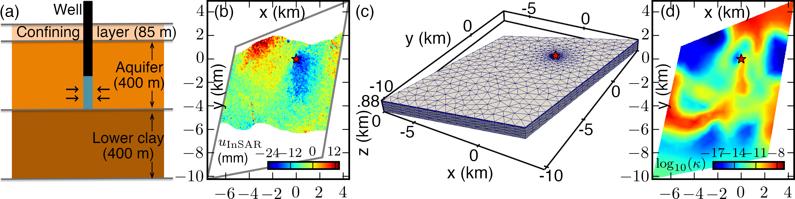
Figure 1: Overview of the Nevada test case. (a) A conceptual illustration of the aquifer model. The well is screened in the lowest half of the aquifer (blue segment). (b) InSAR-observed LOS deformation (east, north, and vertical displacements projected onto the radar line-of-sight) between May 4, 2003 and October 26, 2003 over the study area. (c) The computational mesh we use to model the aquifer. The mesh has 4,081 nodes. (d) Two-dimensional horizontal slice of the inferred permeability, $e^{\mathbf{m}_{\text{MAP}}}$, at mid-aquifer depth (in decimal logarithm) using InSAR data in Figure 1b and the mesh in Figure 1c. In panels (b)–(d), $x$ is the east direction and $y$ is the north direction relative to the well location $(x,y)=(0,0)$ (marked by the red star).

3.1 Study Site, InSAR Deformation Data, and Aquifer Computational Model

Our study site is located southeast of Mesquite, Nevada. The aquifer is $\sim$ 400 m thick, which is confined by an $\sim$ 85 m thick brittle layer at the top and a clay layer that is at least 400 m thick at the bottom (Figure 1a). A controlled aquifer test was performed at a newly installed municipal well WX31 between May 7, 2003 and July 9, 2003 [Burbey (2006)]. This well pumped 9,028 m³ of GW per day during the study period, and it was relatively isolated from other wells in the area. The regional GW recharge is due mainly to winter precipitation in the surrounding mountains, which was negligible during the summer pumping test. Burbey06 analyzed the aquifer geomechanical response to the pumping test using InSAR and GPS data. They found significant deviations between the observed deformation pattern and the expected deformation pattern from a homogeneous aquifer. This finding motivates us to investigate the lateral permeability heterogeneity of the aquifer using the Bayesian framework.

We processed an Envisat interferogram (05/04/2003-10/26/2003) that captures the surface deformation associated with the pumping test along the radar LOS direction (Figure 1b). Here the LOS unit look vector is $\alpha_{\text{LOS}}=[0.381,-0.08,0.921]$ (refer to section 2.2 for definition), which means that the measured LOS deformation $\mathbf{d}^{\text{obs}}$ is mostly sensitive to vertical motion ($\alpha_{3}\approx 1$). The observed deformation pattern (Figure 1b) shows a subsidence bowl that is shifted toward the southeast of the well and an uplift signal in the northwest of the domain. The latter is likely due to a fault existence northwest the well [Burbey (2008), Alghamdi . (2020)]. We found that the noise in the Envisat interferogram is mainly due to phase decorrelation that is uncorrelated in space ($\sigma_{\text{InSAR}}=3.2$ mm). Thus we chose the noise covariance operator $\mathbf{\Gamma}_{\text{noise}}$ to be a diagonal matrix with diagonal values $\sigma_{\text{InSAR}}^{2}$.

Our aquifer model is described in detail in AlghamdiHesseChenEtAl2020A, we assume a 3D poroelastic medium governed by the Biot model (1) and represent the pumping well as a volumetric sink term $f_{p}$. The parameter values of the forward model (1) are provided in Table 2 and based on previously estimated values by Burbey06. We discretized the model (Figure 1a) using a 4,081-node unstructured tetrahedral layered mesh (Figure 1c). The discretization on this mesh results in a total of ${n_{\text{state}}=72,980}$ pressure, displacement, and fluid flux DOFs per time step. We additionally created finer meshes of 16,896 and 67,133 nodes, which result in ${n_{\text{state}}=320,824}$ and ${n_{\text{state}}=1,322,067}$, respectively, for the purpose of studying the eigenvalues decay of the prior-preconditioned data misfit Hessian $\mathbf{\Gamma}_{\text{prior}}\mathbf{H}_{\text{misfit}}$.

We imposed zero normal displacement at the bottom boundary, zero displacement at the lateral boundaries, no traction at the top boundary, and no GW flux at all boundaries. Under the assumption of zero initial deviation from the hydrostatic pressure everywhere in the domain at $t=0$, we ran the model for $T=175$ days using 154 variable-length time steps. Initial time steps are 1.2 hours to capture rapid pressure decay that occurs after the onset of pumping and increased gradually to reach five days toward the end of the simulation. Each time step involves solving a linear system of size $n_{\text{state}}$.

3.2 Estimating the Permeability MAP Point using the Bayesian Framework

Based on a heuristic approach [Alghamdi . (2020)], we chose the weakest bilaplacian-like Matérn class prior that yet sufficiently regularizes the inverse problem to allow the (Gauss–)Newton method to converge (defined as reducing the gradient norm by four orders of magnitude). The average-over-domain pointwise standard deviation (SD) of this prior is $\sim 1.5$ in decimal logarithm, and its mean is the constant permeability value estimated by Burbey08 as shown in Table 2. The spatial correlation length of the permeability values in these samples is $\rho=2$ km in the lateral direction and an order of magnitude larger in the vertical direction. The latter constraint inhibits permeability variations in the vertical direction. We impose this constraint because (1) vertical variations are likely not informed by deformation data obtained on the surface; (2) the large aspect ratio of the aquifer horizontal-to-vertical dimensions leads to predominantly horizontal flow.

In the Part I paper [Alghamdi . (2020)], we used the InSAR surface deformation data (Figure 1b) to solve for the permeability realization that is most likely to be the true permeability field. This is known as the maximum a posteriori (MAP) point of the posterior distribution (Equation (7)). We found that the MAP point (Figure 1d) reveals distinct features in the lateral permeability field: high permeability channel extending from south the well to the southwest and low permeability barrier to the northwest of the well. We validated the InSAR-based permeability MAP point solution using an independent GPS data set as well as a synthesized data set. We computed the MAP point using (Gauss–)Newton method and observed a mesh-independent convergence. We also demonstrated the consistency of the solution with respect to a wide range of prior assumptions, and InSAR data multi-look choices, given a consistent data noise treatment.

3.3 Creating Low-Rank Based Laplace Approximation of the Posterior and MCMC Sampling

The Bayesian inversion framework allows us to quantify the uncertainty in the solution by sampling the posterior distribution. To estimate the uncertainty in the aquifer permeability, we first build the low-rank based Laplace approximation $\pi_{\text{Laplace,r}}$ of the posterior, a process that entails solving the generalized eigenvalue problem (15) using a randomized generalized eigensolver [Villa . (2020)], to obtain the low-rank based approximation of posterior covariance matrix (16). We study two approximations in which we use truncation values $r=80$ and $r=150$, respectively. This low-rank based Laplace approximation is feasible to compute—it mainly costs $O(r)$ incremental forward (27) and incremental adjoint (28) solves—and can serve (depending on how close the parameter to observable map is to a linear one) as a good approximation of the posterior distribution $\pi_{\text{post}}$. Additionally, we use this approximation in the gpCN proposal (see Algorithm 1) to sample the true posterior.

To that end, we generate five MCMC chains, using the gpCN MCMC method (Algorithm 1), each of length 50,000, with additional 1,000 burn-in samples. Each chain start point $\boldsymbol{\eta}_{\text{post}}^{(0)}$ is an independent sample from the low-rank based Laplace approximation $\pi_{\text{Laplace,r}}$, with $r=80$. We similarly generate two pCN chains [Cotter . (2012)]. Generating a single gpCN chain (and similarly a pCN chain) costs 50,000 forward solves of the system (1), discretized on the 4,081-node mesh. These solves are required to evaluate the ratio $\alpha_{\text{gpCN}}$ in Algorithm 1. We store pressure $p$ and displacement $\mathbf{u}$ solutions evaluated at time $t_{\text{InSAR}}\approx 5.7$ months, the time at which the LOS deformation (Figure 1b) is observed relative to the start of the simulation, for different realizations of $\mathbf{m}$. We set the step size $\beta=0.25$ in gpCN proposal formula (18) and set $\beta=0.01$ in pCN proposal. These values were found with a trial-and-error approach to balance between high acceptance rate and large step size. To compare several posterior-based QoI vs prior-based QoI, we generate 1,000 samples from the prior distribution and the low-rank based Laplace approximation (with $r=80$) directly and solve the system (1) at each sample. We carry out the implementation using the FEniCS library for finite element discretization in space [Logg . (2012)] and the hIPPYlib library for state-of-the-art Bayesian and deterministic PDE-constrained inversion algorithms [Villa . (2018)].

4 Results and Discussion

Here we first establish the low rank property of the data misfit Hessian for the Nevada test-case poroelasticity problem introduced in section 4.1. This property is critical for the applicability of the gpCN algorithm. Then we study the convergence and mixing of the gpCN algorithm and compare it to the performance of the pCN algorithm in section 4.2. Finally, we use the gpCN algorithm to quantify the uncertainty in the aquifer permeability and state variables QoI, given the InSAR data information, in sections 4.3 and 4.4.

4.1 The Prior Preconditioned Data Misfit Hessian Spectrum

The plausibility of the low-rank based Laplace approximation and the computational feasibility of the gpCN method, discussed in sections 2.3 and 2.4, rely on the inherent low rank structure of the data misfit Hessian. This property allows for truncating the low-rank based Laplace approximation at $r\ll n_{n}$. In section 2.3 we proved that this property holds for an idealized 1D poroelasticity problem. To demonstrate this property for the 3D Nevada test problem introduced in section 3 we computed the eigenvalues and eigendirections of the prior-preconditioned data misfit Hessian evaluated at the MAP point (Figure 2). The bottom right panel shows the decay of the eigenvalues on increasingly refined meshes. The decay patterns in the 16,896-node and 67,133-node meshes are almost identical, which demonstrates a mesh-independent eigenvalue decay on sufficiently resolved meshes. On all three meshes, only about $r=70$–$80\ll n_{n}$ eigenvalues are larger than one, and therefore, only the $r$ eigendirections that correspond to these eigenvalues can be inferred from InSAR data with high confidence. Selected eigendirections are shown in Figure 2. Similar to the 1D problem in section 2.3, the larger the eigenvalue the smoother the corresponding eigendirection, indicating that it is easier to infer smooth modes. The distinctive features of the first few eigendirections, which are inferred strongly from the data, are localized near the well and the surrounding subsidence bowl, where surface deformation is largest.

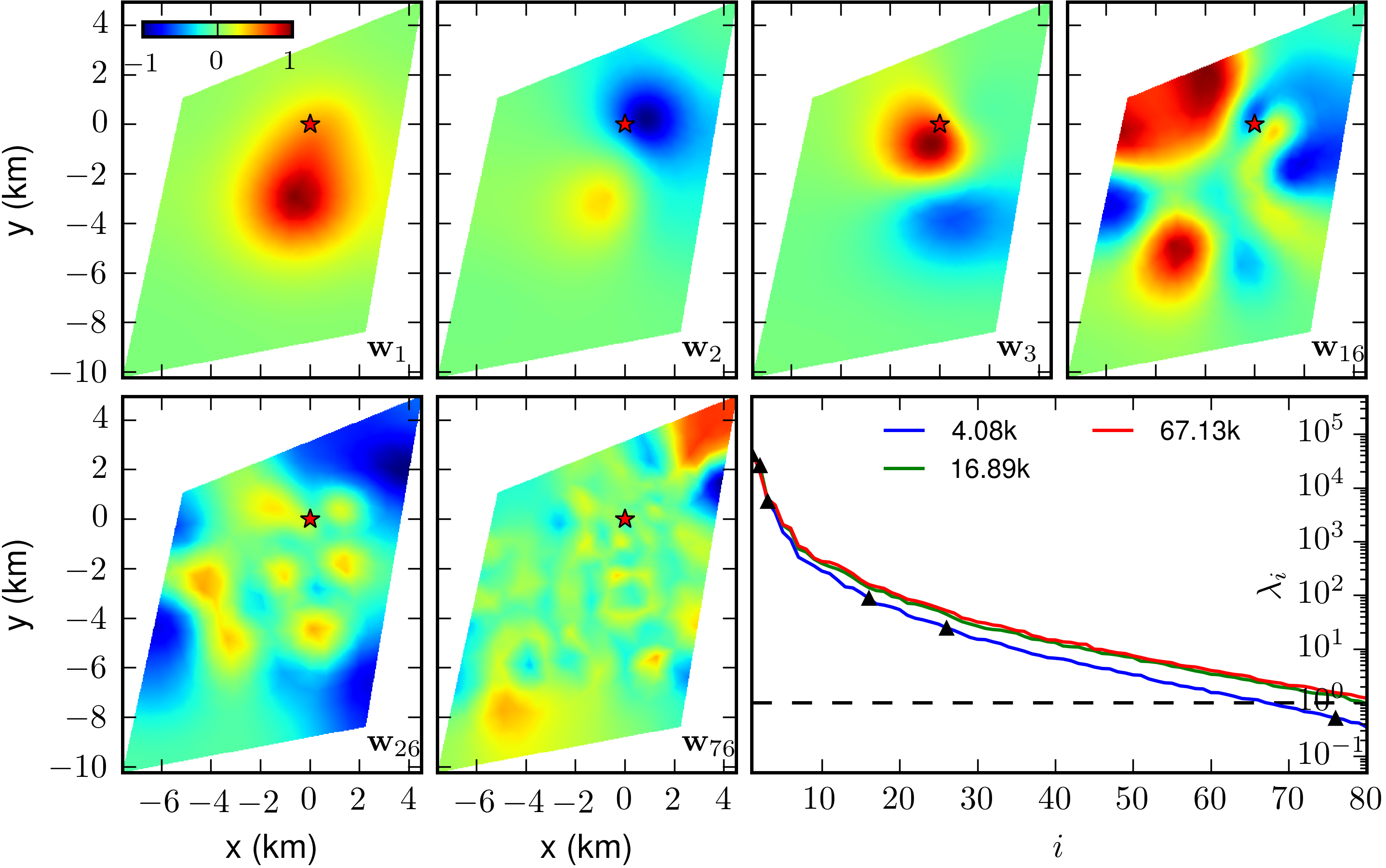
Figure 2: Eigenvectors $\mathbf{w}_{i}$ for ${i=1,2,3,16,26,76}$ of the generalized eigenproblem (15) using InSAR data and the $4{,}081$-node mesh. (Bottom right panel) Eigenvalues of the data misfit Hessian using the 4,081-node (blue), the 16,896-node (green), and the 67,133-node (red) meshes. The black dashed line is ${\lambda_{i}=1}$. The eigenvalues corresponding to the eigenvectors $\mathbf{w}_{i}$ for ${i=1,2,3,16,26,76}$ in the $4{,}081$-node mesh are marked by black triangles. In all meshes, only $\sim$70–80 eigendirections can be inferred from the data (i.e. those inferred with high confidence, corresponding to $\lambda_{i}>1$).

4.2 Performance of the gpCN algorithm

For uncertainty quantification in realistic 3D transient multi-physics problems it is essential to improve the sampling of the parameter space. Incorporating log posterior Hessian information in gpCN proposal, through the low-rank based Laplace approximation, leads to better convergence properties, compared to the pCN algorithm, see Table 1 for methods performance. The gpCN algorithm achieves an acceptance rate of $\sim 22\%$ when using a step size $\beta=0.25$. To achieve a similar acceptance rate for the pCN algorithm, $\sim 24\%$, a much smaller number $\beta=0.01$ is required, which leads to smaller MCMC steps and slower exploration of the feasible parameter space. Consequently, the sample autocorrelation in gpCN chains decays much faster than in pCN chains, as shown in the bottom right panel in Figure 3. The large step-size in gpCN chains increases the number of independent MCMC samples and leads to a larger effective sample size compared to pCN chains (Table 1). Visualizing chains mixing at selected points in space (Figure 3) highlights the performance difference between the two methods. The pCN chains vary slowly, fail to converge and do not explore the feasible parameter space while gpCN chains move more rapidly and exhibit more of a “fuzzy worm” pattern [Bui-Thanh (2012)] in which correlation between samples is weaker.

Table 1: pCN and gpCN performance

Method	# chainsa	PDE solves per chain	$\beta$	Acceptance rate	IATb	ESS/chainc
pCN	2	50,000	$0.01$	$\sim 24\%$	9754	5
gpCN	5	50,000	$0.25$	$\sim 22\%$	494	101
a Each chain is of length 50,000 samples.
b IAT is the pointwise integrated autocorrelation time reported as average over the domain and over the number of chains.
c $\text{ESS}=\frac{\text{Chain length}}{\text{IAT}}$ is the effective sample size.

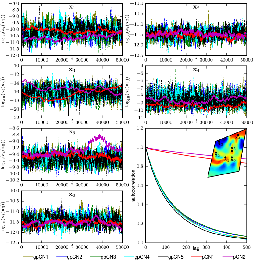
Figure 3: pCN and gpCN chains mixing at selected points in space $\mathbf{x}_{1}=(-2.0,-4.0,0.6)$, $\mathbf{x}_{2}=(-5.0,-2.5,0.6)$, $\mathbf{x}_{3}=(-4.0,1.0,0.6)$, $\mathbf{x}_{4}=(2.0,3.0,0.6)$, $\mathbf{x}_{5}=(0,-2.0,0.6)$, and $\mathbf{x}_{6}=(0,-4.0,0.6)$ in km. (Bottom right panel) autocorrelation versus lag. Autocorrelation values are reported as average over the domain. The two pCN chains and the five gpCN chains are labeled pCN1, pCN2, and gpCN1–gpCN5, respectively.

4.3 Uncertainty Quantification of the Aquifer Permeability

In this section we present the solution of the Bayesian inverse problem through the variance, samples, and selected marginal distributions of the permeability posterior distribution. In particular we study both the low-rank based Laplace approximation and the MCMC-based posterior distributions.

4.3.1 Permeability Pointwise Standard Deviation and Samples

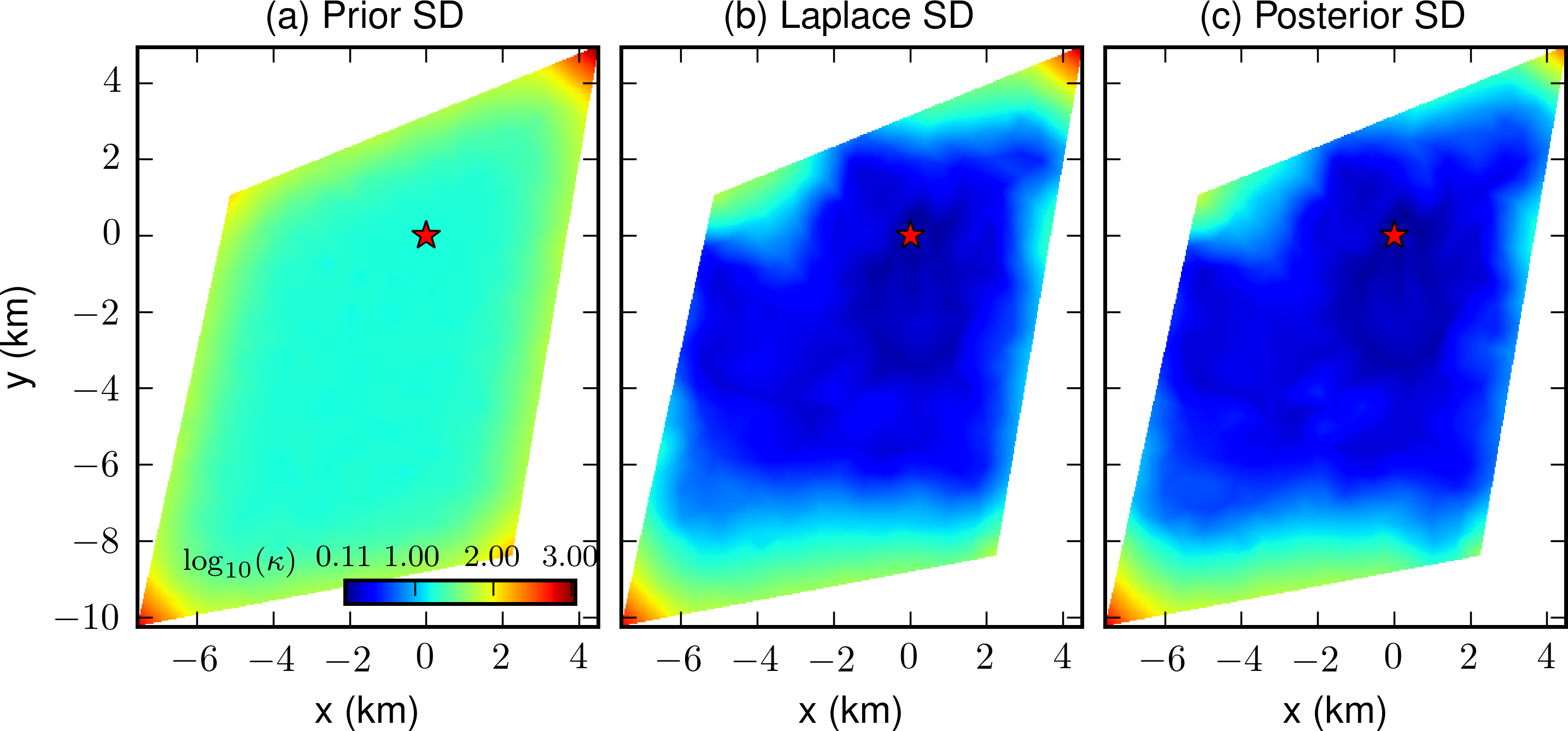
Figure 4: Two-dimensional horizontal slices of the permeability pointwise standard deviation (in decimal logarithm) at mid-aquifer depth of (a) the prior distribution, (b) the low-rank based Laplace approximation ($r=80$), and (c) the MCMC-based true posterior. In all the panels, $x$ is the east direction and $y$ is the north direction relative to the well location $(x,y)=(0,0)$ (marked by the red star).

The posterior distribution incorporates information from InSAR data and the aquifer model. This significantly reduces the pointwise standard deviation (SD) of the permeability posterior distributions compared to the prior pointwise SD in most of the domain. Figure 4 shows this is the case for both the low-rank based Laplace approximation and the MCMC-based posterior. The spatial variation of the SD inferred from the low-rank based Laplace approximation in panel 4b is very similar to the SD of the MCMC-based true posterior distribution in panel 4c. The MCMC-based true posterior, however, infers a slightly larger area where permeability can be inferred with high confidence. This is also reflected in the samples obtained from these three distributions. Samples from the prior distribution exhibit varying random patterns (Figure 5a) whereas samples from the low-rank based Laplace approximation and the MCMC-based true posterior (Figure 5b and 5c) show consistent features, e.g. a low permeability area northwest the well and a high permeability channel extending toward the south/southwest. In the latter two distributions, permeability patterns at the southern part of the domain display more randomness than in the center and the north. This randomness is expected because the SD at the southern part is relatively larger (Figures 4b and 4c) and is likely a result of two factors, the southern part of the domain is far from the major part of the subsidence bowl, and the InSAR data we use in the inversion does not cover that area of the domain.

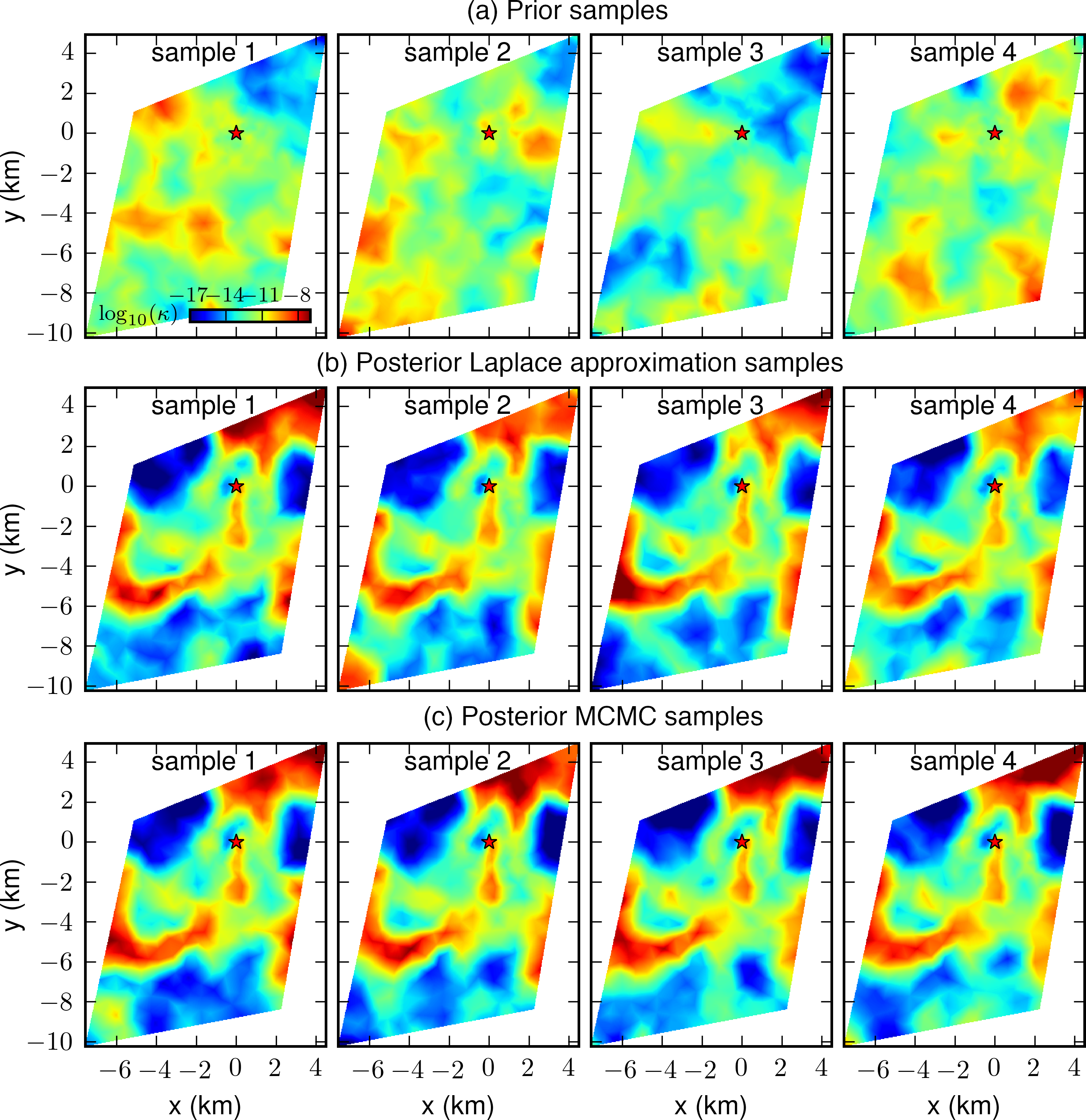
Figure 5: Two-dimensional horizontal slices of permeability samples (in decimal logarithm) at mid-aquifer depth from (a) the prior distribution, (b) the low-rank based posterior Laplace approximation ($r=80$), and (c) the true posterior distribution (MCMC samples).

4.3.2 Location-wise Permeability PDF Marginals

To illustrate the broad range of results we compare 1D marginals of the prior distribution to posterior distributions inferred using both the low-rank based Laplace approximation and MCMC at selected points in the domain ($\mathbf{x}_{i}$ for $i=1,2,...,6$ in Figure 6). The posterior distributions inferred from the Laplace approximations with $r=80$ and $r=150$ modes are very similar. This demonstrates that most of the information from the data is contained in the first 80 modes and adding the next 70 modes in the low-rank based Laplace approximation provides only limited additional information. The marginals of the MCMC-based true posterior distribution at points $\mathbf{x}_{i}$ are obtained by applying 1D Gaussian kernel density estimation (KDE) to the pointwise values of the MCMC samples at $\mathbf{x}_{i}$. These marginals confirm the observation from the pointwise SD values (Figure 4) that the posterior distribution is significantly narrower than the prior distribution. Moreover, the pointwise marginals reveal that the MCMC-based true posterior exhibits more certainty in the permeability inference compared to the low-rank based Laplace approximation in most of the selected pointwise locations ($\mathbf{x}_{2}$ to $\mathbf{x}_{6}$).

The certainty in the inferred permeability varies with location in the domain as shown in Figure 6. We notice, for example, inference with high certainty at the location $\mathbf{x}_{5}$, which is located in the high permeability channel extending south from the well and within the subsidence bowl. On the other hand, the existence of a low permeability region northwest of the well reduces the GW flux and increases the uncertainty in the parameters in the region beyond this flow barrier, for example at location $\mathbf{x}_{3}$. This effect was also observed by HesseStadler14 in synthetic model problems and we refer to it here as the shadowed region. The uncertainty in the permeability of the shadowed region is large, because in the absence of flow there is no surface deformation that informs the model permeability in this region.

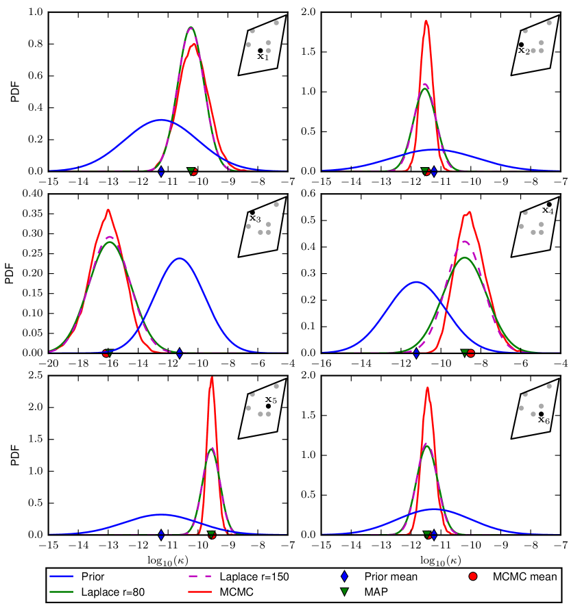
Figure 6: One-dimensional marginals at selected points $\mathbf{x}_{i}$ for $i=1,2,...,6$ (coordinates are provided in Figure 3) of the prior distribution, the low-rank based Laplace approximation (using $r=80$ and $r=150$), and the MCMC-based true posterior distribution.

Slight deviation of the MCMC-based true posterior from a Gaussian distribution can be observed from the posterior two-dimensional marginals (see Figure 7). The mean of the marginals at $\{\mathbf{x}_{4},\mathbf{x}_{1}\}$ and $\{\mathbf{x}_{3},\mathbf{x}_{4}\}$ is different from the MAP point and the distribution displays right-skewness of the marginal at $\{\mathbf{x}_{3},\mathbf{x}_{4}\}$. On the whole though, the deviations of the MCMC-based true posterior from Gaussian distribution are minor in this particular case.

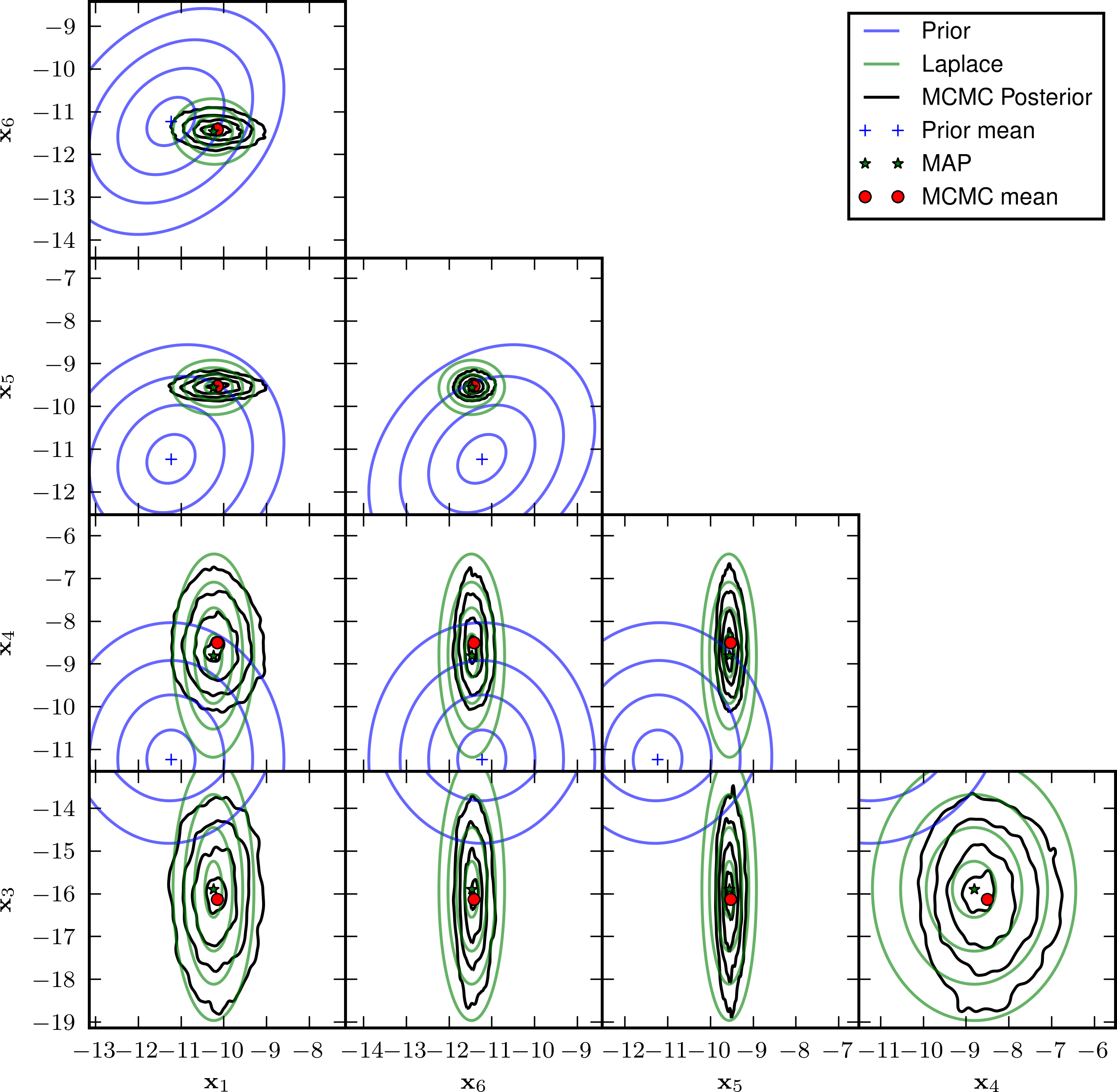
Figure 7: Two-dimensional marginals at selected pairs of points in space $\{\mathbf{x}_{i},\mathbf{x}_{j}\}$ for $i,j=1,3,4,5,6$ and $i\neq j$ (coordinates are provided in Figure 3) of the prior, the low-rank based Laplace approximation ($r=80$), and the MCMC-based true posterior. The values of the contour lines of each distribution are $c_{\text{cl}}\times\max(\Pi)$ for $c_{\text{cl}}=0.1,0.3,0.6,0.9$, where $\Pi$ is the distribution PDF.

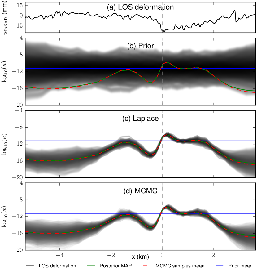
Figure 8: Prior, low-rank based Laplace approximation, and true posterior marginals over a line. (a) InSAR LOS deformation signal over a line segment $l_{1}$ parallel to the $x$ axes, extends from the west to the east of the domain, and passes by the well location at the surface. Marginal distributions, over a line segment $l_{2}$ parallel to the $x$ axes, extends from the west to the east of the domain, and passes by the well location at $z=.6$ km, computed from (b) the prior, (c) the low-rank based Laplace approximation, and (d) the MCMC-based true posterior. We apply KDE to pointwise values of the samples at evenly spaced 1,000 grid points of $l_{2}$ to generate the approximate marginal PDFs. The gray shade is proportional to the PDF value. Values of the estimated PDF beyond the shaded area are negligible. The well location is marked with a gray dotted vertical line and the prior mean, the MAP point, and the MCMC samples mean are shown in blue, green and dotted red, respectively (in decimal logarithm).

Figure 8 shows marginals over a line segment parallel to the $x$ axes that extends from the west to the east of the domain and passes by the well at point $(x,y,z)=(0,0,.6\text{ km})$. We observe that, compared to the prior distribution (Figure 8b), the posterior distributions characterize the permeability with much more certainty especially in the middle part of the line segment near the well from $\sim-2$ to $\sim 2$ km (Figures 8c and 8d). This is mainly because this interval coincides with significant deformation signal or deformation gradient (Figure 8a). In particular, the sharp drop in the permeability just west to the well location is inferred with very high certainty as evident by the narrow marginal distribution at that location. The location of this feature coincides with large gradient in the subsidence from almost no deformation just west to the well to significant subsidence at and east to the well. This demonstrates that large gradients in the deformation data inform the permeability characterization strongly.

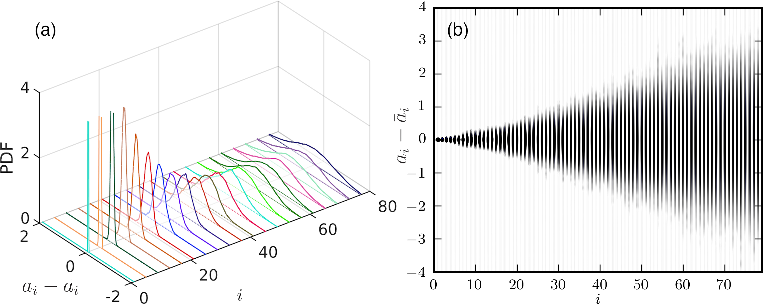
Figure 9: Marginal distributions of the gpCN MCMC samples components $a_{i}$ in the first $r=80$ eigendirections $\mathbf{w}_{i}$, for $i=1,2,...,r$. The PDFs are shifted by their means $\bar{a}_{i}$. (a) PDFs of $a_{i}$ (for better visualization, we display only every fourth PDF and truncate the PDF plot at $\text{PDF}=4$). (b) PDFs of $a_{i}$ are plotted vertically in gray scale. The darker the gray shade, the higher the PDF value. Values of the estimated PDF beyond the shaded area are negligible (less than $\sim.0003$).

4.3.3 Permeability PDF Marginals Over the Eigendirections $\mathbf{w}_{i}$

In the preceding discussion, we studied the permeability characterization location-wise in the physical domain. Uncertainty in the permeability characterization can be viewed from a different perspective, in the directions of the parameter space that are determined by the generalized eigenvalue problem (15) [Petra . (2014)]. To that end, we compute the marginals of the MCMC-based posterior distribution in the first $r=80$ eigendirections $\mathbf{w}_{i}$ (we show selected directions in Figure 2). We denote with $a_{i}$, for $i=1,2,...,r$, the components of the $j^{\text{th}}$ MCMC sample $\boldsymbol{\eta}_{\text{post}}^{(j)}$ in the eigendirections $\mathbf{w}_{i}$, $j=0,1,...,n_{s}$ where $n_{s}=250,000$ is the total number of gpCN MCMC samples. We can write the sample $\boldsymbol{\eta}_{\text{post}}^{(j)}$ as a linear combination of the eigendirections $\mathbf{w}_{i}$ as follows:

$$\boldsymbol{\eta}_{\text{post}}^{(j)}=\sum_{i=1}^{n_{n}}a_{i}\mathbf{w}_{i}$$ (19)

Using the $\mathbf{\Gamma}_{\text{prior}}^{-1}$-orthogonality of the directions $\mathbf{w}_{i}$, the components $a_{i}$ are given by $a_{i}=\mathbf{w}_{i}^{T}\mathbf{\Gamma}_{\text{prior}}^{-1}\boldsymbol{\eta}_{\text{post}}^{(j)}$. We use 1D Gaussian KDE to approximate the distribution of each component $a_{i}$ over the samples $\boldsymbol{\eta}_{\text{post}}^{(j)}$ for $j=0,1,...,n_{s}$. We show $a_{i}$ distributions in Figure 9, shifted by their averages $\bar{a}_{i}$ for ease of comparison. We notice that, as expected, the more dominant the eigendirection in the generalized eigenvalue problem (15), the more certain the inference of the component in that direction. The first few directions, in particular, are inferred with significantly high confidence. We also observe that the distributions of some $a_{i}$’s deviate slightly from a Gaussian distribution showing a mild skewness.

4.4 Uncertainty Quantification of the State Variables

Quantifying the propagation of uncertainty in the parameters to the state variables QoIs, e.g. pore pressure and total subsidence, is of interest in GW management applications [Qin . (2018)]. We show the prior and posterior predictive distributions of the pressure $p(\mathbf{x}_{i},t_{\text{InSAR}})$, at the well location $\mathbf{x}_{0}=(0,0,.6)$, and locations $\mathbf{x}_{1},\mathbf{x}_{2},\mathbf{x}_{4}$ and $\mathbf{x}_{4}$ (coordinates are provided in Figure 3) in Figure 10. We also show these predictive distributions for total subsidence volume $-\int_{\Gamma^{\text{top}}}u_{3}(t_{\text{InSAR}})ds$, where $\Gamma^{\text{top}}$ is the domain top surface (bottom panel in Figure 10). We use KDE to estimate the PDF of each of those QoIs. We note that these distributions can be highly non-Gaussian and that the prior-based distributions vary across a much wider range compared to the narrow posterior-based distributions. In some locations, $\mathbf{x}_{1}$, $\mathbf{x}_{2}$ and $\mathbf{x}_{5}$ for example, relying only on prior knowledge significantly underestimates the expected pressure drop; the posterior-based QoI mean at these locations is considerably larger in magnitude than that of the prior-based QoI. We also note appreciable differences between the low-rank based Laplace approximation and the MCMC based posterior predictives. The mixing behaviour of the chains for these QoIs distributions (shown in Figure 11) is similar to what was observed for the parameter chains in section 4.2.

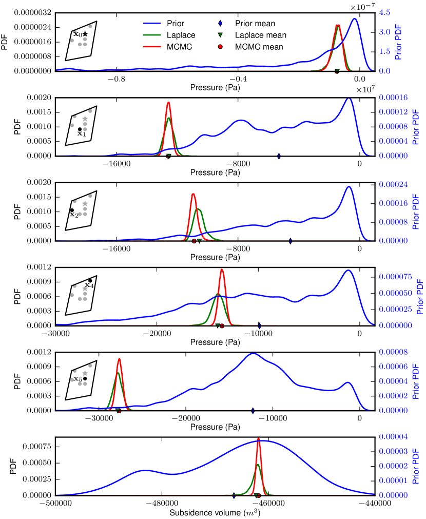
Figure 10: Prior, low-rank based Laplace approximation, and MCMC-based posterior predictives for pointwise pressure values at selected locations ($\mathbf{x}_{0},\mathbf{x}_{1},\mathbf{x}_{2},\mathbf{x}_{4}$, and $\mathbf{x}_{5}$) and total subsidence volume (bottom panel). In all panels, the values of the Laplace approximation-based and MCMC-based PDFs are measured by the left $y$-axis scale while the right $y$-axis scale measures the prior PDF.

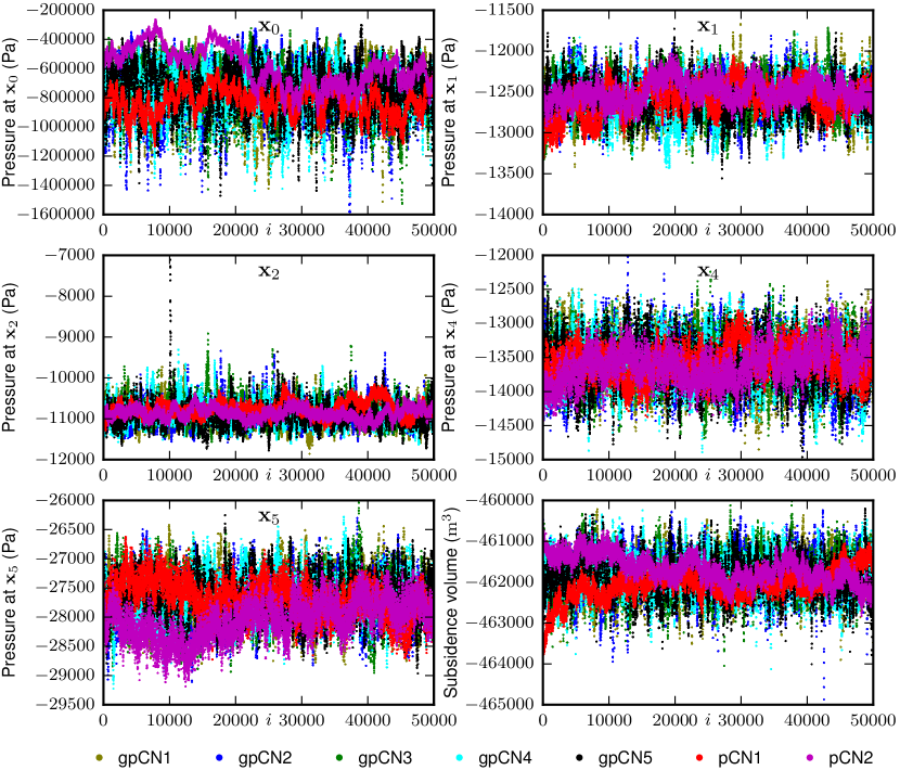
Figure 11: pCN and gpCN MCMC-based mixing of the pointwise pressure values at selected locations ($\mathbf{x}_{0},\mathbf{x}_{1},\mathbf{x}_{2},\mathbf{x}_{4}$, and $\mathbf{x}_{5}$) and total subsidence volume (bottom right panel). The two pCN chains and the five gpCN chains are labeled pCN1, pCN2, and gpCN1–gpCN5, respectively.

5 Conclusion

The use of InSAR surface deformation data to quantify the uncertainty in GW aquifer models via solution of poroelasticity-governed high dimensional Bayesian inverse problems is important for data-driven, model-predictive management of GW resources. The intrinsic low dimensionality of this inverse problem, evident by the rapid decay in data misfit Hessian eigenfunctions, makes solving this problem computationally tractable when the right computational tools are used, e.g. our proposed gpCN MCMC method employing low-rank-based Laplace approximation proposals, scalable priors based on inverses of differential operators, and an inexact Newton method with adjoint-based gradients and Hessian actions to find the MAP point. The use of these tools guarantees that the number of forward poroelasticity PDE solves required to solve the inverse problem is independent of the parameter dimension. In the Nevada test case, for example, only $r\approx 80$ (out of $n_{n}=4{,}081$) directions are sufficient to construct the low-rank based Laplace approximation.

The information content of InSAR data is rich enough to enable characterizing the permeability and state variable derived QoI with high certainty. Location-wise, the permeability in the aquifer in regions that undergo a detectable subsidence signal or large subsidence gradient is inferred with narrow variance. However, what can be inferred about areas that are “shadowed” from the source (well WX31) beyond a flow barrier is very limited. The update in the prior statistical characterization of selected state variable derived QoI via learning from InSAR data is also critical. Our results show for example that relying on prior knowledge alone leads to underestimating the pressure drop in some locations.

Appendix A Adjoint-Based Derivation of the Hessian Operator

We derive the Hessian operator in the Newton iteration that we form for finding the MAP point. Maximizing the posterior distribution (7) with respect to the parameter $\mathbf{m}$ to find the MAP point is equivalent to minimizing the negative log posterior, i.e.

$$\min_{\mathbf{m}\in{\rm I\!R}^{n_{n}}}\mathcal{J}(\mathbf{m})=\frac{1}{2}(\mathbf{\bar{B}}\mathbf{\bar{X}}- \mathbf{d}^{\text{obs}})^{T}\mathbf{\Gamma}_{\text{noise}}^{-1}(\mathbf{\bar{B}}\mathbf{\bar{X}}-\mathbf{d}^{\text{obs}})+\frac{1}{2}(\mathbf{m}-\bar{\mathbf{m}})^{T}\mathbf{\Gamma}_{\text{prior}}^{-1}(\mathbf{m}-\bar{\mathbf{m}}),$$ (20)

where $\mathbf{\bar{X}}$ depends on $\mathbf{m}$ through the solution of the forward problem $\mathbf{\bar{S}}(\mathbf{m})\mathbf{\bar{X}}=\mathbf{\bar{F}}$.

To derive the gradient using the adjoint method, we form the Lagrangian for the constrained optimization problem (20) to be:

$$\mathcal{L}(\mathbf{m},\mathbf{\bar{X}},\mathbf{\bar{Y}})= \frac{1}{2}(\mathbf{\bar{B}}\mathbf{\bar{X}}-\mathbf{d}^{\text{obs}})^{T}\mathbf{\Gamma}_{\text{noise}}^{-1}(\mathbf{\bar{B}}\mathbf{\bar{X}}-\mathbf{d}^{\text{obs}})$$

$$+ \frac{1}{2}(\mathbf{m}-\bar{\mathbf{m}})^{T}\mathbf{\Gamma}_{\text{prior}}^{-1}(\mathbf{m}-\bar{\mathbf{m}})+\mathbf{\bar{Y}}^{T}(\mathbf{\bar{S}}(\mathbf{m})\mathbf{\bar{X}}-\mathbf{\bar{F}}).$$ (21)

where $\mathbf{\bar{Y}}$ is the Lagrange multiplier (also called the adjoint variable).

At a minimum of (21), the partial derivatives of the Lagrangian with respect to the state variable, ${\partial\mathcal{L}}/{\partial\mathbf{\bar{X}}}$, the parameter, ${\partial\mathcal{L}}/{\partial\mathbf{m}}$, and the adjoint variable, ${\partial\mathcal{L}}/{\partial\mathbf{\bar{Y}}}$, vanish. We set ${\partial\mathcal{L}}/{\partial\mathbf{\bar{X}}}$ and ${\partial\mathcal{L}}/{\partial\mathbf{\bar{Y}}}$ to zero, which gives the state equation and the adjoint equation respectively:

$$\frac{\partial\mathcal{L}}{\partial\mathbf{\bar{Y}}}(\mathbf{\bar{X}},\mathbf{\bar{Y}},\mathbf{m})= \mathbf{\bar{S}}(\mathbf{m})\mathbf{\bar{X}}-\mathbf{\bar{F}}=0\quad\text{(state)},$$ (22)

$$\frac{\partial\mathcal{L}}{\partial\mathbf{\bar{X}}}(\mathbf{\bar{X}},\mathbf{\bar{Y}},\mathbf{m})= \mathbf{\bar{B}}^{T}\mathbf{\Gamma}_{\text{noise}}^{-1}(\mathbf{\bar{B}}\mathbf{\bar{X}}-\mathbf{d}^{\text{obs}})+\mathbf{\bar{S}}^{T}(\mathbf{m})\mathbf{\bar{Y}}=0\quad\text{(adjoint)}.$$ (23)

We satisfy these two conditions by solving the discretized state and adjoint equations exactly for the given value of $\mathbf{m}$. Thus we seek the parameter $\mathbf{m}$ that ensures that the gradient

$$\frac{\partial\mathcal{L}}{\partial\mathbf{m}}(\mathbf{\bar{X}},\mathbf{\bar{Y}},\mathbf{m})= \mathbf{\Gamma}_{\text{prior}}^{-1}(\mathbf{m}-\bar{\mathbf{m}})+\mathbf{\bar{C}}^{T}(\mathbf{m})\mathbf{\bar{Y}}$$ (24)

vanishes. The operator $\mathbf{\bar{C}}$ is the partial derivative (sensitivity) of the residual $\mathcal{R}=\mathbf{\bar{S}}\mathbf{\bar{X}}-\mathbf{\bar{F}}$ with respect to the parameter $\mathbf{m}$

$$\mathbf{\bar{C}}=\frac{\partial}{\partial\mathbf{m}}(\mathbf{\bar{S}}\mathbf{\bar{X}}-\mathbf{\bar{F}})=\frac{\partial}{\partial\mathbf{m}}(\mathbf{\bar{S}}\mathbf{\bar{X}}).$$ (25)

We solve the equation ${\partial\mathcal{L}}/{\partial\mathbf{m}}=0$ using Newton’s method.

To derive the Newton iteration we form the Lagrangian $\mathcal{L}_{\mathcal{H}}$:

$$\mathcal{L}_{\mathcal{H}}:= {\delta\mathbf{\bar{X}}}^{T}\left(\mathbf{\bar{B}}^{T}\mathbf{\Gamma}_{\text{noise}}^{-1}(\mathbf{\bar{B}}\mathbf{\bar{X}}-\mathbf{d}^{\text{obs}})+\mathbf{\bar{S}}^{T}(\mathbf{m})\mathbf{\bar{Y}}\right)$$

$$+ {\delta\mathbf{\bar{Y}}}^{T}\big{(}\mathbf{\bar{S}}(\mathbf{m})\mathbf{\bar{X}}-\mathbf{\bar{F}}\big{)}$$

$$+ {\delta\mathbf{m}}^{T}\big{(}\mathbf{\Gamma}_{\text{prior}}^{-1}(\mathbf{m}-\bar{\mathbf{m}})+\mathbf{\bar{C}}^{T}(\mathbf{m})\mathbf{\bar{Y}}\big{)},$$ (26)

where $\delta\mathbf{\bar{X}}$ and $\delta\mathbf{\bar{Y}}$ are Lagrange multipliers for the adjoint (23) and state (22) equations, and $\delta\mathbf{m}$ is the direction in which the Hessian acts. The so-called incremental forward and incremental adjoint problems are defined as follows:

$$\frac{\partial\mathcal{L}_{\mathcal{H}}}{\partial\mathbf{\bar{Y}}} =\mathbf{\bar{S}}(\mathbf{m}){\delta\mathbf{\bar{X}}}+\mathbf{\bar{C}}(\mathbf{m}){\delta\mathbf{m}}=0.\quad\text{(incremental forward)},$$ (27)

$$\frac{\partial\mathcal{L}_{\mathcal{H}}}{\partial\mathbf{\bar{X}}} =\mathbf{\bar{B}}^{T}\mathbf{\Gamma}_{\text{noise}}^{-1}\mathbf{\bar{B}}{\delta\mathbf{\bar{X}}}+\mathbf{\bar{S}}^{T}(\mathbf{m}){\delta\mathbf{\bar{Y}}}+\Big{(}\frac{\partial}{\partial\mathbf{\bar{X}}}(\mathbf{\bar{C}}^{T}(\mathbf{m})\mathbf{\bar{Y}})\Big{)}^{T}\delta\mathbf{m}$$

$$=\mathbf{W}_{\mathbf{\bar{X}}\mathbf{\bar{X}}}{\delta\mathbf{\bar{X}}}+\mathbf{\bar{S}}^{T}(\mathbf{m}){\delta\mathbf{\bar{Y}}}+\mathbf{W}_{\mathbf{\bar{X}}\mathbf{m}}(\mathbf{m})\delta\mathbf{m}=0.\quad\text{(incremental adjoint)}$$ (28)

The Hessian action in the direction $\delta\mathbf{m}$ is given by:

$$\frac{\partial\mathcal{L}_{\mathcal{H}}}{\partial\mathbf{m}} =\frac{\partial}{\partial\mathbf{m}}({\delta\mathbf{\bar{X}}}^{T}\mathbf{\bar{S}}^{T}(\mathbf{m})\mathbf{\bar{Y}})+\frac{\partial}{\partial\mathbf{m}}({\delta\mathbf{\bar{Y}}}^{T}\mathbf{\bar{S}}(\mathbf{m})\mathbf{\bar{X}})+\mathbf{\Gamma}_{\text{prior}}^{-1}\delta\mathbf{m}+\frac{\partial}{\partial\mathbf{m}}({\delta\mathbf{m}}^{T}\mathbf{\bar{C}}^{T}(\mathbf{m})\mathbf{\bar{Y}})$$

$$=\mathbf{W}_{\mathbf{m}\mathbf{\bar{X}}}(\mathbf{m})\delta\mathbf{\bar{X}}+\mathbf{\bar{C}}^{T}(\mathbf{m})\delta\mathbf{\bar{Y}}+\mathbf{\Gamma}_{\text{prior}}^{-1}\delta\mathbf{m}+\mathbf{R}_{\mathbf{m}\mathbf{m}}(\mathbf{m})\delta\mathbf{m}.$$ (29)

Substituting the solutions for $\delta\mathbf{\bar{X}}$ and $\delta\mathbf{\bar{Y}}$ from the systems (27) and (28) into the expression (29) gives the Hessian expression:

$$\mathbf{H}(\mathbf{m})= \mathbf{\Gamma}_{\text{prior}}^{-1}+\mathbf{H}_{\text{misfit}}(\mathbf{m}),$$ (30)

where

$$\mathbf{H}_{\text{misfit}}(\mathbf{m})\coloneqq \mathbf{R}_{\mathbf{m}\mathbf{m}}(\mathbf{m})+\mathbf{\bar{C}}^{T}(\mathbf{m})\mathbf{\bar{S}}^{-T}(\mathbf{m})(\mathbf{W}_{\mathbf{\bar{X}}\mathbf{\bar{X}}}\mathbf{\bar{S}}^{-1}(\mathbf{m})\mathbf{\bar{C}}(\mathbf{m})-\mathbf{W}_{\mathbf{\bar{X}}\mathbf{m}}(\mathbf{m}))$$

$$-\mathbf{W}_{\mathbf{m}\mathbf{\bar{X}}}(\mathbf{m})\mathbf{\bar{S}}^{-1}(\mathbf{m})\mathbf{\bar{C}}(\mathbf{m}).$$ (31)

The matrices $\mathbf{W}_{\mathbf{\bar{X}}\mathbf{\bar{X}}},\mathbf{W}_{\mathbf{\bar{X}}\mathbf{m}},\mathbf{W}_{\mathbf{m}\mathbf{\bar{X}}}$, and $\mathbf{R}_{\mathbf{m}\mathbf{m}}$ are defined as follows

$$\mathbf{W}_{\mathbf{\bar{X}}\mathbf{\bar{X}}}=\mathbf{\bar{B}}^{T}\mathbf{\Gamma}_{\text{noise}}^{-1}\mathbf{\bar{B}},\ \mathbf{W}_{\mathbf{\bar{X}}\mathbf{m}}=\frac{\partial}{\partial\mathbf{m}}(\mathbf{\bar{S}}^{T}\mathbf{\bar{Y}}),\ \mathbf{W}_{\mathbf{m}\mathbf{\bar{X}}}=\frac{\partial}{\partial\mathbf{\bar{X}}}(\mathbf{\bar{C}}^{T}\mathbf{\bar{Y}}),\ \mathbf{R}_{\mathbf{m}\mathbf{m}}=\frac{\partial}{\partial\mathbf{m}}(\mathbf{\bar{C}}^{T}\mathbf{\bar{Y}}).$$

Forming the Hessian, evaluated at a given $\mathbf{m}$, explicitly, requires applying the operator $\mathbf{\bar{S}}^{-1}$ to each column of $\mathbf{\bar{C}}$ to form the matrices product $\mathbf{\bar{S}}^{-1}\mathbf{\bar{C}}$. Applying the operator $\mathbf{\bar{S}}^{-1}$ to a vector amounts to an incremental forward poroelasticity solve, equation (27). Therefore, forming the GN Hessian explicitly costs $n_{n}$ poroelasticity PDEs solves (note that no additional solves are required for forming the product $\mathbf{\bar{C}}^{T}\mathbf{\bar{S}}^{-T}$ since it is the transpose of the product $\mathbf{\bar{S}}^{-1}\mathbf{\bar{C}}$). However, applying $\mathbf{H}$ to a direction mainly costs applying the operators $\mathbf{\bar{S}}^{-1}$ and $\mathbf{\bar{S}}^{-T}$ each to a vector which is the cost of two poroelasticity PDEs solves (one incremental forward (27) and one incremental adjoint (28)).

Appendix B Forward Model Parameters

Table 2: Forward model parameters

(a) Model parameters

Volumetric force ($\mathbf{f_{u}}$)	0
Pumping rate ($-\int_{\Omega}f_{p}\mathrm{d}\mathbf{x}$)	$9{,}028$ $\text{m}^{3}/\text{day}$
Fluid viscosity ($\mu$)	$0.001$ $\text{Pa}\cdot\text{s}$
Biot-Willis coefficient ($\alpha$)	$0.998$
Height of the domain ($h$)	$885$ m
Water density ($\rho$)	$997.97$ $\text{Kg}/\text{m}^{3}$
Gravitational acceleration ($g$)	$9.8$ $\text{m}/\text{s}^{2}$
Water compressibility ($\beta_{w}$)	$4.4\times 10^{-10}$ $\text{Pa}^{-1}$

(b) Layer parameters

	Units	Aquifer	Confining layer	Lower clay
Poisson’s ratio ($\nu$)	-	$0.25$	$0.25$	$0.25$
Drained shear modulus ($G$)	Pa	$3.4\times 10^{8}$	$3.5\times 10^{8}$	$8\times 10^{8}$
Specific storage ($S_{\epsilon}$)	$\text{Pa}^{-1}$	$2.1\times 10^{-9}$	$1.2\times 10^{-9}$	$1.2\times 10^{-9}$
Prior mean value ($\text{log}_{10}(\kappa)$)	$\text{m}^{2}$ (for $\kappa$)	-11.2	-14.2	-14.2