Learning the exchange-correlation functional from nature with fully differentiable density functional theory

Abstract

Improving the predictive capability of molecular properties in ab initio simulations is essential for advanced material discovery. Despite recent progress making use of machine learning, utilizing deep neural networks to improve quantum chemistry modelling remains severely limited by the scarcity and heterogeneity of appropriate experimental data. Here we show how training a neural network to replace the exchange-correlation functional within a fully-differentiable three-dimensional Kohn-Sham density functional theory (DFT) framework can greatly improve simulation accuracy. Using only eight experimental data points on diatomic molecules, our trained exchange-correlation networks enable improved prediction accuracy of atomization energies across a collection of 104 molecules containing new bonds and atoms that are not present in the training dataset.

Fast and accurate predictive models of atomic and molecular properties are key in advancing novel material discovery. With the rapid development of machine learning (ML) techniques, considerable effort has been dedicated to accelerating predictive simulations, enabling the efficient exploration of configuration space. Much of this work focuses on end-to-end ML approaches gilmer2017-neural-message-passing , where the models are trained to predict some specific molecular or material property using tens to hundreds of thousands of data points, generated via simulations schutt2018schnet . Once trained, ML models have the advantage of accurately predicting the simulation outputs much faster than the original simulations smith2017ani-1 . The level of accuracy achieved by ML models with respect to the simulated data can be very high, and may even reach chemical accuracy on select systems outside the original training dataset faber2017prediction-ml-better . Although these machine learning approaches show considerable promise, they rely heavily on the availability of large datasets for training.

While there has been a concerted effort in accelerating predictive models, less attention has been dedicated to using machine learning to increase the accuracy of the model itself with respect to the experimental data. In particular, as ML models typically rely on some underlying simulation for the training data, the trained models can never exceed the simulations in terms of accuracy. However, training ML models using experimental data is challenging as the available data is highly heterogeneous as well as limited, making it difficult to train accurate ML models tailored to reproducing a specific system or physical property. This limitation also poses a great challenge to the generalization capability of ML models to systems outside the training data.

One emerging solution to this problems is to use machine learning to build models which learn the exchange-correlation (xc) functional within the framework of Density Functional Theory (DFT) snyder2012ml-xc ; lei2019design-xc ; nagai2020completing ; dick2020mlxc ; li2021kohn-sham-regularizer ; chen2020deepks . Here, the Kohn-Sham scheme (KS-DFT) hohenberg1964inhomogeneous ; kohn1965self-ks can be used to calculate various ground-state properties of molecules and materials, the accuracy of which largely depends on the quality of the employed xc functional. Work along these lines in the one-dimensional case show promise snyder2012ml-xc ; li2021kohn-sham-regularizer , but are severely limited by the lack of availability of experimental data for one-dimensional systems. An alternative approach is to learn the xc functional using a dataset constructed from electron density profiles obtained from coupled-cluster (CCSD) simulations vcivzek1966correlation-ccsd , and the xc energy densities obtained from an inverse Kohn-Sham scheme kanungo2019exact-inverse-ks . However, this method is fundamentally limited to, at most, match the accuracy of the original simulations. Recently, Nagai et al. nagai2020completing reported on successfully representing the xc functional as a neural network, trained to fit 2 different properties of 3 molecules using the three-dimensional KS-DFT calculation in PySCF sun2018pyscf via gradient-less optimization. While their results show promise in predicting various material properties, gradient-less methods in training neural networks typically suffer from bad convergence maheswaranathan2019guided-es and are too computationally intensive to scale to larger and more complex neural networks.

In this context, we present here a new machine learning approach to learn the xc functional using heterogeneous experimental data. We achieve this by incorporating a deep neural network representing the xc functional in a fully differentiable three-dimensional KS-DFT calculation. In our method, the xc functional is represented by a network that takes the three-dimensional electron density profile as its input and produces the xc energy density as its output. Notably, using a xc neural network (XCNN) in a fully differentiable KS-DFT calculation gives us a framework to train the xc functional using any available experimental properties, however heterogeneous, which can be simulated via standard KS-DFT. Moreover, as the neural network is independent of the specific physical system (atom type, structure, number of electrons, etc.), a well-trained XCNN should be generalizable to a wide range of systems, including those outside the pool of training data. In this paper, we demonstrate this approach using a dataset comprising atoms and molecules from the first few rows of the periodic table, but the results are readily extendable to more complex structures.

A critical part of realizing our method is writing a KS-DFT code in a fully differentiable manner. This is achieved here by writing the KS-DFT code using an automatic differentiation library, PyTorch neurips2019-pytorch , and by providing separately the gradients of all the KS-DFT components which are not available in PyTorch. The KS-DFT calculation involves self-consistent iterations of solving the Kohn-Sham equations,

$$H[n](\mathbf{r})\phi_{i}(\mathbf{r}) =\varepsilon_{i}\phi_{i}(\mathbf{r}),$$ (1)

$$n(\mathbf{r}) =\sum_{i}f_{i}|\phi_{i}(\mathbf{r})|^{2},$$ (2)

where $n(\mathbf{r})$ is the electron density as a function of a 3D coordinate ($\mathbf{r}$), $f_{i}$ is the occupation number of the $i$-th orbital ($\phi_{i}$), $\varepsilon_{i}$ is the Kohn-Sham orbital energy, and $H[n](\mathbf{r})$ is the Hamiltonian operator, a functional of the electron density profile $n$ and a function of the 3D coordinate. The Hamiltonian operator is given in atomic units as $H[n](\mathbf{r})=-\nabla^{2}/2+v(\mathbf{r})+v_{H}[n](\mathbf{r})+v_{xc}[n](\mathbf{r})$ with $-\nabla^{2}/2$ representing the kinetic operator, $v(\mathbf{r})$ the external potential operator including ionic Coulomb potentials, $v_{H}[n](\mathbf{r})$ the Hartree potential operator, and $v_{xc}[n](\mathbf{r})$ the xc potential operator. The xc potential operator is defined as the functional derivative of the xc energy with respect to the density, i.e. $v_{xc}[n](\mathbf{r})=\delta E_{xc}[n]/\delta n(\mathbf{r})$.

In this work, the orbitals in the above equations are represented using contracted Gaussian-type orbital basis sets pritchard2019new-bse , $b_{j}(\mathbf{r})$ for $j=\{1...n_{b}\}$ where $n_{b}$ is the number of basis elements. As the basis set is non-orthogonal, Eq. (1) becomes the Roothaan’s equation roothaan1951new ,

$$\mathbf{F}[n]\mathbf{p}_{i}=\varepsilon_{i}\mathbf{Sp}_{i},$$ (3)

where $\mathbf{p}_{i}$ is the basis coefficient for the $i$-th orbital, $\mathbf{S}$ is the overlap matrix with elements $S_{rc}=\int b_{r}(\mathbf{r})b_{c}^{*}(\mathbf{r})\mathrm{d}\mathbf{r}$, and $\mathbf{F}[n]$ is the Fock matrix as a functional of the electron density profile, $n$, with elements $F_{rc}=\int b_{r}(\mathbf{r})H[n](\mathbf{r})b_{c}^{*}(\mathbf{r})\mathrm{d}\mathbf{r}$. Unless specified otherwise, all calculations involved in this paper use 6-311++G(3pd,3df) basis sets clark1983efficient-pople-set .

Equation (3) can be solved by performing an eigendecomposition of the Fock matrix to obtain the orbitals from the electron density profile. The ionic Coulomb potential, Hartree potential, and the kinetic energy operators in the Fock matrix are constructed by calculating the Gaussian integrals with libcint sun2015libcint . The contribution from the xc potential operator in the Fock matrix is constructed by integrating it with the basis using the SG-3 integration grid dasgupta2017standard-sg3 , with Becke scheme to combine multi-atomic grids becke1988multicenter . The KS-DFT calculation proceeds by solving Eq. (3) and computing Eq. (2) iteratively until convergence or self-consistency is reached. The schematics of our differentiable KS-DFT code is shown in Fig. 1.

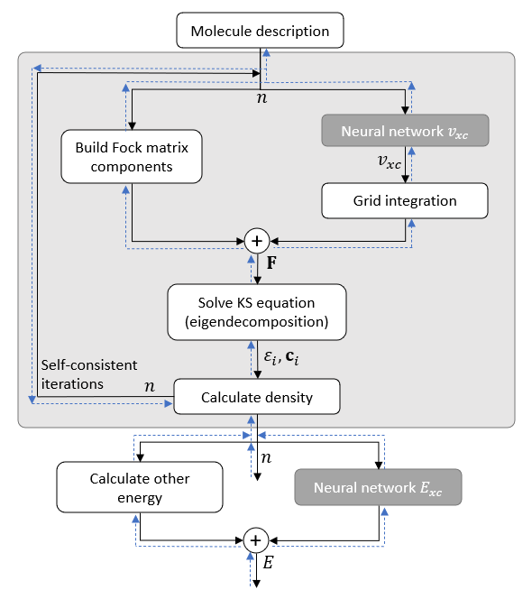
Figure 1: Schematics of the xc neural network and differentiable KS-DFT code. The trainable neural network is illustrated with darker gray boxes. The solid dark lines show the forward calculation flow while the dashed blue lines show the gradient backpropagation flow.

Although modern automatic differentiation libraries provide many operations that enable an automatic propagation of gradient calculations, there are many gradient operations that have to be implemented specifically for this project. An important example is the self-consistent cycle iteration. Previous approaches employed a fixed number of linear mixing iterations to achieve self-consistency, and let the automatic differentiation library propagate the gradient through the chain of iterations tamayo2018automatic-diffiqult ; li2021kohn-sham-regularizer . In contrast, we implement the gradient propagation of the self-consistency cycle using an implicit gradient calculation (see supplementary materials), allowing us to deploy a better self-consistent algorithm, achieving faster and more robust convergence than linear mixing. We implemented the gradient calculation of the self-consistency cycle in xitorch kasim2020xitorch , a publicly available computational library written specifically for this project.

Another example is the gradient calculation of the eigendecomposition with (near-)degenerate eigenvalues. This often produces numerical instabilities in the gradient calculation. To solve this problem, we follow the calculation by Kasim kasim2020derivatives-degen to obtain a numerically stable gradient calculation in cases of (near-)degeneracy, which is also implemented in xitorch. Other parts in KS-DFT that require specific gradient implementations are the calculation of the xc energy, the Gaussian basis evaluation, and the Gaussian integrals. The details of the gradient calculations in these cases can be found in the supplementary materials.

With the fully differentiable KS-DFT code to hand, the xc energy represented by a deep neural network can be trained efficiently. For this work we will test two different types of xc deep neural networks (XCNN) based on two rungs of Jacob’s ladder – the Local Density Approximation (LDA) and the Generalized Gradient Approximation (GGA). These xc energies can be written as:

$$E_{\rm nnLDA}[n] =\alpha E_{\rm LDA(xc)}[n]+\beta\int n(\mathbf{r})f(n,\xi)\ \mathrm{d}\mathbf{r}$$ (4)

$$E_{\rm nnPBE}[n] =\alpha E_{\rm PBE(xc)}[n]+\beta\int n(\mathbf{r})f(n,\xi,s)\ \mathrm{d}\mathbf{r},$$ (5)

where $E_{\rm LDA(xc)}$ is the LDA exchange kohn1965self-ks and correlation energy perdew1992accurate-pw92 , and $E_{\rm PBE(xc)}$ is the PBE exchange-correlation energy perdew1996generalized-gga-pbe . Here $\alpha$ and $\beta$ are two tunable parameters, and $f(\cdot)$ is the trainable neural network. The LDA and PBE energies are calculated using Libxc lehtola2018recent and wrapped with PyTorch to provide the required gradient calculations.

The XCNNs take inputs of the local electron density $n$, the relative spin polarization $\xi=(n_{\uparrow}-n_{\downarrow})/n$, and the normalized density gradient $s=|\nabla n|/(24\pi^{2}n^{4})^{1/3}$ perdew1996generalized-gga-pbe . The neural network is an ordinary feed-forward neural network with 3 hidden layers consist of 32 elements each with a softplus nair2010rectified-relu-softplus activation function to ensure infinite differentiability of the neural network. To avoid non-convergence of the self-consistent iterations during the training, the parameters $\alpha$ and $\beta$ are initialized to have values of 1 and 0 respectively.

For the XCNN training, we compiled a small dataset consisting of experimental atomization energies (AE) from the NIST CCCBDB database NIST_CCCBDB , atomic ionization potentials (IP) from the NIST ASD database NIST_ASD , and calculated density profiles using a CCSD calculation vcivzek1966correlation-ccsd . The calculated density profiles are used as a regularization to ensure that the learned xc does not produce electron densities that are too far from CCSD predictions, a concern discussed by Medvedev et al. medvedev2017density-deviate .

The dataset is split into 2 groups: training and validation. The training dataset is used directly to update the parameters of the neural network via the gradient of a loss function (see supplementary materials for details on the loss function). After the training is finished, we selected a model checkpoint during the training that gives the lowest loss function for the validation dataset.

The complete list of atoms and molecules used in the training and validation datasets is shown in Table 1. Importantly, the size of the dataset used in this work is orders of magnitude smaller than datasets used in most ML-related work present in the literature on predicting molecular properties ramakrishnan2014quantum-qm9 ; chmiela2017machine-md17 ; brockherde2017bypassing-ks . We note that some atoms are only present in the validation set and not in the training set, to include checkpoints that are able to generalize well to new types of atoms outside the training set.

Table 1: Atoms and molecules presented in the training and validation datasets.

Type	Atomization energy	Density profile	Ionization potential
Training	H2, LiH, O2, CO	H, Li, Ne, H2, Li2, LiH, B2, O2, CO	O, Ne
Validation	N2, NO, F2, HF	He, Be, N, N2, F2, HF	N, F

Table 2: Mean absolute error (MAE) in kcal/mol of the atomization energy and ionization potential for atoms and molecules in the test dataset. The column “IP 18” represents the deviation in ionization potential for atoms H-Ar. Column “AE 104” is the MAE of atomization energy of a collection of 104 molecules from ref. curtiss1997assessment-g2 . Column “DP 99” is the difference of the density profile (in $\times 10^{-3}$ Bohr^-3) for the 104 molecules, excluding 5 molecules that have multiple possible density profiles. The following 4 columns present the atomization energies of subsets of molecules from the full 104-molecule set: “AE 16 HC” for 16 hydrocarbons, “AE 25 subs HC” for 25 substituted hydrocarbons, “AE 34 others-1” for 34 non-hydrocarbon molecules containing only first and second row atoms, and “AE 30 others-2” for 30 non-hydrocarbon molecules containing at least one third row atom. The suffix “-IP” in the XCNN calculation indicates that the xc neural networks were trained with the ionization potential dataset. The bolded values are the best MAE in the respective column for each group of approximations.

Calculation	IP 18	AE 104	DP 99	AE 16 HC	AE 25 subs HC	AE 33 others-1	AE 30 others-2
Local density approximations (LDA)
LDA (exchange only)	24.6	28.2	25.7	48.7	29.0	25.4	19.8
LDA (PW92 perdew1992accurate-pw92 )	6.9	70.5	23.3	97.0	101.1	58.8	43.7
XCNN-LDA	50.8	15.5	10.9	22.7	19.4	7.8	16.6
XCNN-LDA-IP	15.2	18.5	9.8	25.4	21.8	8.4	22.9
Generalized gradient approximations (GGA)
PBE perdew1996generalized-gga-pbe	3.6	16.5	2.6	15.1	23.2	18.0	9.8
XCNN-PBE	10.7	7.4	2.4	5.4	8.4	6.5	8.5
XCNN-PBE-IP	4.1	8.1	2.4	6.8	9.6	6.7	8.6
Other approximations
SCAN sun2015strongly-scan	3.7	5.0	1.1	3.8	8.2	4.0	4.6
CCSD (basis: cc-pvqz dunning1989gaussian-ccpvqz )	2.0	12.1	0.0	11.1	17.7	11.2	9.0
CCSD(T) (basis: cc-pvqz)	1.3	3.5	N/A	2.2	5.6	2.5	3.5

To test the performance of the trained XCNNs, we prepared a test dataset consisting of the atomization energies of 104 molecules from ref. curtiss1997assessment-g2 , and the ionization potentials of atoms H-Ar. The experimental geometric data as well as the atomization energies for the 104 molecules were obtained from the NIST CCCBDB database NIST_CCCBDB , while the ionization potentials are obtained from the NIST ASD database NIST_ASD (see supplementary materials for the details in compiling the datasets). There are actually 146 molecules in ref. curtiss1997assessment-g2 , however, only 104 molecules have experimental data in CCCBDB, so we limit our dataset to those. While each molecule in the training and validation datasets only contain 2 atoms from the first two rows of the periodic table (i.e. H-Ne), molecules in the test dataset contain 2-14 atoms from the first three rows of the periodic table (i.e. H-Ar). A complete list of all the molecules used in the test dataset can be found in the supplementary materials.

Our first experiment is done by training the XCNN without the ionization potential dataset, i.e., using only atomization energies and density profile data. The results are presented in Table 2. We see that in this case both XCNN-LDA and XCNN-PBE provide significant improvement over their bases, i.e. LDA and PBE, respectively. In terms of average atomization energy prediction errors across the 104 test molecules, XCNN-LDA achieves more than 4 times lower error than LDA (PW92) and XCNN-PBE achieves more than 2 times lower error than PBE. Importantly, although the training and validation sets contain atomization energies only for 8 diatomic molecules, both XCNNs provide improvements on atomization energy predictions of the 104-molecule test dataset, which includes molecules with up to 14 atoms.

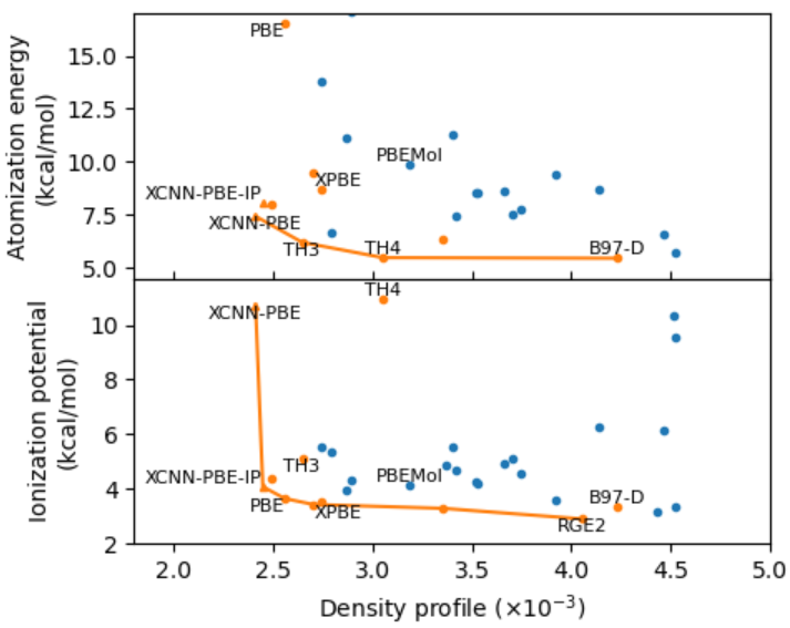
Figure 2: Objective plots for GGA functionals. The orange data points are the functionals that lie on the Pareto front for the 3 objectives (atomization energy, density profile, ionization energy). The orange line shows the Pareto front on 2 objectives in the respective plots. XCNN-PBE and XCNN-PBE-IP are shown by the orange triangle which also lies on the Pareto front. The full list can be found in the supplementary materials. Only functionals with deviations within the range are shown for clarity.

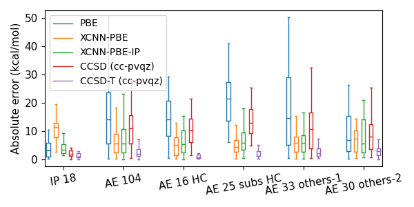
Figure 3: Statistical comparison of PBE, XCNN-PBE, CCSD, and CCSD(T) for each group. The line in the box represents the median of the absolute error. For clarity, outliers are not shown.

By looking into the subsets of the atomization energy dataset, both XCNN-LDA and XCNN-PBE also achieve better atomization energy predictions than their bases on all of the subsets. The substantial improvements seen on the hydrocarbon and substituted hydrocarbon molecules show the generalization capability of the technique to molecules with bonds not present in neither the training nor the validation dataset (e.g., C–H, C–C, C=C). Moreover, both XCNNs can also predict better atomization energy on the “AE-30 others-2” subset containing third-row atoms that are not present in the training and validation datasets. The improvement of atomization energy predictions on unseen atoms and bonds demonstrate a very promising generalization capability of the machine learning models outside the training distribution.

Despite these encouraging results on the atomization energies, both XCNNs lead to significantly worse predictions of atomic ionization potentials compared with their bases. Therefore, for the next experiment we trained the XCNN by adding ionization potential data into the training and validation datasets, as shown in Tab. 1. The xc neural networks trained with this additional data are called “XCNN-LDA-IP” and “XCNN-PBE-IP”. Adding ionization potential data to the training and validation datasets improves the performance of XCNNs on the ionization potential at the cost of slightly increasing the error on the atomization energy predictions. Although the ionization potential predictions of XCNN-IPs do not have lower error compared to their bases, they produce considerably better predictions on the atomization energies of the tested molecules than their bases.

When compared to other 48 GGAs on XCNN-PBE and XCNN-PBE-IP give the lowest errors on density profiles deviation. Moreover, when comparing on atomization energy, density profile, and ionization potential, both XCNN-PBEs lie on the Pareto front as can be seen in Figure 2. This means that there is no other GGAs that can provide improvement on all aspects considered in this paper. Detailed results on GGAs comparison can be seen in the supplementary materials.

Another interesting result is that even though CCSD simulation is used in the training and validation datasets, the trained XCNN-PBE can achieve considerably better predictions on atomization energies than CCSD. A detailed comparison of our XCNN-PBE results with CCSD calculations is presented in Fig. 3. We see that the results from XCNN-PBE are in most cases better than calculations based on CCSD. This result highlights a key advantage of our method over other ML-based methods that rely fully on simulation data: as our method utilizes heterogeneous experimental data in the training, it enables us to learn xc functionals that can exceed in accuracy even the simulations used to train them.

Although the trained XCNNs cannot make better predictions than higher level of approximations, e.g. SCAN sun2015strongly-scan and CCSD(T), the presented method shows that significant improvement can be made within the same level of approximation. The level of accuracy can be improved in the future work by using a higher level of approximation, such as moving to the higher rungs of Jacob’s ladder or incorporating more global density information with neural networks in calculating the xc energy. While perfectly viable within our framework, such investigations remain outside the scope of the current paper.

We presented a novel approach to train machine-learned xc functionals within the framework of fully-differential Kohn-Sham DFT using experimental data. Our xc neural networks, trained on a few atoms and diatomic molecules, are able to improve the prediction of atomization and ionization energies across a set of 104 molecules, including larger molecules containing atoms and bonds not present in the training dataset. We have limited our study to a minimal training dataset and to a relatively small neural network, but our results are readily extendable to substantially larger systems, bigger experimental datasets, additional heterogeneous physics quantities, and to the use of more sophisticated neural networks. This demonstration of experimental-data-driven xc functional learning, embedded within a differentiable DFT simulator, shows great promise to advance computational material discovery. The codes can be found in kasim2020-xitorch ; kasim2021-dqc ; kasim2021-xcnn .

- (1) Justin Gilmer, Samuel S Schoenholz, Patrick F Riley, Oriol Vinyals, and George E Dahl. Neural message passing for quantum chemistry. In International Conference on Machine Learning, pages 1263–1272. PMLR, 2017.
- (2) Kristof T Schütt, Huziel E Sauceda, P-J Kindermans, Alexandre Tkatchenko, and K-R Müller. Schnet–a deep learning architecture for molecules and materials. The Journal of Chemical Physics, 148(24):241722, 2018.
- (3) Justin S Smith, Olexandr Isayev, and Adrian E Roitberg. Ani-1: an extensible neural network potential with dft accuracy at force field computational cost. Chemical science, 8(4):3192–3203, 2017.
- (4) Felix A Faber, Luke Hutchison, Bing Huang, Justin Gilmer, Samuel S Schoenholz, George E Dahl, Oriol Vinyals, Steven Kearnes, Patrick F Riley, and O Anatole Von Lilienfeld. Prediction errors of molecular machine learning models lower than hybrid dft error. Journal of chemical theory and computation, 13(11):5255–5264, 2017.
- (5) John C Snyder, Matthias Rupp, Katja Hansen, Klaus-Robert Müller, and Kieron Burke. Finding density functionals with machine learning. Physical review letters, 108(25):253002, 2012.
- (6) Xiangyun Lei and Andrew J Medford. Design and analysis of machine learning exchange-correlation functionals via rotationally invariant convolutional descriptors. Physical Review Materials, 3(6):063801, 2019.
- (7) Ryo Nagai, Ryosuke Akashi, and Osamu Sugino. Completing density functional theory by machine learning hidden messages from molecules. npj Computational Materials, 6(1):1–8, 2020.
- (8) Sebastian Dick and Marivi Fernandez-Serra. Machine learning accurate exchange and correlation functionals of the electronic density. Nature communications, 11(1):1–10, 2020.
- (9) Li Li, Stephan Hoyer, Ryan Pederson, Ruoxi Sun, Ekin D Cubuk, Patrick Riley, and Kieron Burke. Kohn-sham equations as regularizer: Building prior knowledge into machine-learned physics. Physical Review Letters, 126(3):036401, 2021.
- (10) Yixiao Chen, Linfeng Zhang, Han Wang, and Weinan E. Deepks: A comprehensive data-driven approach toward chemically accurate density functional theory. Journal of Chemical Theory and Computation, 2020.
- (11) Pierre Hohenberg and Walter Kohn. Inhomogeneous electron gas. Physical review, 136(3B):B864, 1964.
- (12) Walter Kohn and Lu Jeu Sham. Self-consistent equations including exchange and correlation effects. Physical review, 140(4A):A1133, 1965.
- (13) Jiří Čížek. On the correlation problem in atomic and molecular systems. calculation of wavefunction components in ursell-type expansion using quantum-field theoretical methods. The Journal of Chemical Physics, 45(11):4256–4266, 1966.
- (14) Bikash Kanungo, Paul M Zimmerman, and Vikram Gavini. Exact exchange-correlation potentials from ground-state electron densities. Nature communications, 10(1):1–9, 2019.
- (15) Qiming Sun, Timothy C Berkelbach, Nick S Blunt, George H Booth, Sheng Guo, Zhendong Li, Junzi Liu, James D McClain, Elvira R Sayfutyarova, Sandeep Sharma, et al. Pyscf: the python-based simulations of chemistry framework. Wiley Interdisciplinary Reviews: Computational Molecular Science, 8(1):e1340, 2018.
- (16) Niru Maheswaranathan, Luke Metz, George Tucker, Dami Choi, and Jascha Sohl-Dickstein. Guided evolutionary strategies: Augmenting random search with surrogate gradients. In International Conference on Machine Learning, pages 4264–4273. PMLR, 2019.
- (17) Adam Paszke, Sam Gross, Francisco Massa, Adam Lerer, James Bradbury, Gregory Chanan, Trevor Killeen, Zeming Lin, Natalia Gimelshein, Luca Antiga, Alban Desmaison, Andreas Kopf, Edward Yang, Zachary DeVito, Martin Raison, Alykhan Tejani, Sasank Chilamkurthy, Benoit Steiner, Lu Fang, Junjie Bai, and Soumith Chintala. Pytorch: An imperative style, high-performance deep learning library. In H. Wallach, H. Larochelle, A. Beygelzimer, F. d'Alché-Buc, E. Fox, and R. Garnett, editors, Advances in Neural Information Processing Systems, volume 32, pages 8026–8037. Curran Associates, Inc., 2019.
- (18) Benjamin P Pritchard, Doaa Altarawy, Brett Didier, Tara D Gibson, and Theresa L Windus. New basis set exchange: An open, up-to-date resource for the molecular sciences community. Journal of chemical information and modeling, 59(11):4814–4820, 2019.
- (19) Clemens Carel Johannes Roothaan. New developments in molecular orbital theory. Reviews of modern physics, 23(2):69, 1951.
- (20) Timothy Clark, Jayaraman Chandrasekhar, Günther W Spitznagel, and Paul Von Ragué Schleyer. Efficient diffuse function-augmented basis sets for anion calculations. iii. the 3-21+ g basis set for first-row elements, li–f. Journal of Computational Chemistry, 4(3):294–301, 1983.
- (21) Qiming Sun. Libcint: An efficient general integral library for g aussian basis functions. Journal of computational chemistry, 36(22):1664–1671, 2015.
- (22) Saswata Dasgupta and John M Herbert. Standard grids for high-precision integration of modern density functionals: Sg-2 and sg-3. Journal of computational chemistry, 38(12):869–882, 2017.
- (23) Axel D Becke. A multicenter numerical integration scheme for polyatomic molecules. The Journal of chemical physics, 88(4):2547–2553, 1988.
- (24) Teresa Tamayo-Mendoza, Christoph Kreisbeck, Roland Lindh, and Alán Aspuru-Guzik. Automatic differentiation in quantum chemistry with applications to fully variational hartree–fock. ACS central science, 4(5):559–566, 2018.
- (25) Muhammad F Kasim and Sam M Vinko. -torch: differentiable scientific computing library. arXiv preprint arXiv:2010.01921, 2020.
- (26) Muhammad Firmansyah Kasim. Derivatives of partial eigendecomposition of a real symmetric matrix for degenerate cases. arXiv preprint arXiv:2011.04366, 2020.
- (27) John P Perdew and Yue Wang. Accurate and simple analytic representation of the electron-gas correlation energy. Physical review B, 45(23):13244, 1992.
- (28) John P Perdew, Kieron Burke, and Matthias Ernzerhof. Generalized gradient approximation made simple. Physical review letters, 77(18):3865, 1996.
- (29) Susi Lehtola, Conrad Steigemann, Micael JT Oliveira, and Miguel AL Marques. Recent developments in libxc—a comprehensive library of functionals for density functional theory. SoftwareX, 7:1–5, 2018.
- (30) Vinod Nair and Geoffrey E Hinton. Rectified linear units improve restricted boltzmann machines. In Icml, 2010.
- (31) Editor: R. D. Johnson III. NIST Computational Chemistry Comparison and Benchmark Database. NIST Standard Reference Database Number 101 (Release 21, August 2020), [Online]. Available: https://dx.doi.org/10.18434/T47C7Z. National Institute of Standards and Technology, Gaithersburg, MD., 2020.
- (32) A. Kramida, Yu. Ralchenko, J. Reader, and and NIST ASD Team. NIST Atomic Spectra Database (ver. 5.8), [Online]. Available: https://dx.doi.org/10.18434/T4W30F[2020, October]. National Institute of Standards and Technology, Gaithersburg, MD., 2020.
- (33) Michael G Medvedev, Ivan S Bushmarinov, Jianwei Sun, John P Perdew, and Konstantin A Lyssenko. Density functional theory is straying from the path toward the exact functional. Science, 355(6320):49–52, 2017.
- (34) Raghunathan Ramakrishnan, Pavlo O Dral, Matthias Rupp, and O Anatole von Lilienfeld. Quantum chemistry structures and properties of 134 kilo molecules. Scientific Data, 1, 2014.
- (35) Stefan Chmiela, Alexandre Tkatchenko, Huziel E Sauceda, Igor Poltavsky, Kristof T Schütt, and Klaus-Robert Müller. Machine learning of accurate energy-conserving molecular force fields. Science advances, 3(5):e1603015, 2017.
- (36) Felix Brockherde, Leslie Vogt, Li Li, Mark E Tuckerman, Kieron Burke, and Klaus-Robert Müller. Bypassing the kohn-sham equations with machine learning. Nature communications, 8(1):1–10, 2017.
- (37) Larry A Curtiss, Krishnan Raghavachari, Paul C Redfern, and John A Pople. Assessment of gaussian-2 and density functional theories for the computation of enthalpies of formation. The Journal of Chemical Physics, 106(3):1063–1079, 1997.
- (38) Jianwei Sun, Adrienn Ruzsinszky, and John P Perdew. Strongly constrained and appropriately normed semilocal density functional. Physical review letters, 115(3):036402, 2015.
- (39) Thom H Dunning Jr. Gaussian basis sets for use in correlated molecular calculations. i. the atoms boron through neon and hydrogen. The Journal of chemical physics, 90(2):1007–1023, 1989.
- (40) M.F. Kasim. xitorch: differentiable scientific computing library. https://github.com/xitorch/xitorch, 2020.
- (41) M.F. Kasim. Dqc: Differentiable quantum chemistry. https://github.com/mfkasim1/dqc, 2021.
- (42) M.F. Kasim. Xcnn: xc neural network in differentiable dft. https://github.com/mfkasim1/xcnn, 2021.