Mask-GVAE: Blind Denoising Graphs via Partition

Abstract.

We present Mask-GVAE, a variational generative model for blind denoising large discrete graphs, in which ”blind denoising” means we don’t require any supervision from clean graphs. We focus on recovering graph structures via deleting irrelevant edges and adding missing edges, which has many applications in real-world scenarios, for example, enhancing the quality of connections in a co-authorship network. Mask-GVAE makes use of the robustness in low eigenvectors of graph Laplacian against random noise and decomposes the input graph into several stable clusters. It then harnesses the huge computations by decoding probabilistic smoothed subgraphs in a variational manner. On a wide variety of benchmarks, Mask-GVAE outperforms competing approaches by a significant margin on PSNR and WL similarity.

1. Introduction

Recently, graph learning models (Kipf and Welling, 2017; Wu et al., 2019) have achieved remarkable progress in many graph related tasks. Compared with other machine learning models that build on i.i.d. assumption, graph learning models require as input a more sophisticated graph structure. Meanwhile, how to construct a graph structure from raw data is still an open problem. For instance, in a social network the common practice to construct graph structures is based on observed friendships between users (Li et al., 2019a); in a protein-protein interaction (PPI) network the common practice is based on truncated spatial closeness between proteins (Dobson and Doig, 2003). However, these natural choices of graphs may not necessarily describe well the intrinsic relationships between the node attributes in the data (Dong et al., 2016; Pang and Cheung, 2017), e.g., observed friendship does not indicate true social relationship in a social network (Zhang and Chen, 2018), truncated spatial closeness may incorporate noisy interactions and miss true interactions between proteins in a PPI network (Wang et al., 2018). In this work, we assume we are given a degraded graph structure, e.g., having missing/irrelevant edges. We aim to recover a graph structure that removes irrelevant edges and adds missing edges. As in practice noisy-clean graph pairs are rare (Majumdar, 2018), we propose to de-noise the input noisy graph without any supervision from its clean counterpart, which is referred to as blind graph denoising.

Latent generative models such as variational autoencoders (VAEs) (Kingma and Welling, 2013) have shown impressive performance on denoising images (Im et al., 2017) and speech (Chorowski et al., 2019). As images or speech exist in a continuous space, it is easy to utilize gradient descent weapons to power the denoising process. On the contrary, our problem setting involves a large discrete structure, thus it is challenging to generalize the current deep generative models to our problem setting.

We present Mask-GVAE, the first variational generative model for blind denoising large graphs. A key insight of Mask-GVAE is that graph Laplacian eigenvectors associated with small eigenvalues (low eigenvectors) are stable against random edge perturbations if there is a significant cluster structure (Karrer et al., 2008; Peng and Yoshida, 2020; Eldridge et al., 2018). From another viewpoint, (Huang et al., 2009) finds the stability of low eigenvectors lays the foundation of robustness of spectral clustering (Von Luxburg, 2007). Likewise, many real-world graphs do hold these distinct substructures, e.g., PPI network (Ahn et al., 2010), social network (Li et al., 2019a), and co-authorship network (Zhou et al., 2009). We show an illustrative example in Figure 1. In Mask-GVAE, we first use graph neural networks (GNNs) (Kipf and Welling, 2017; Li et al., 2020a) and normalized cut (Shi and Malik, 2000) for the fast estimation of low eigenvectors, i.e., cluster mask. We then encode the latent variables and generate probabilistic smoothed subgraphs, conditioned on the cluster mask and latent variables. A discrete graph is then sampled upon the denoised subgraphs to circumvent the non-differentiability problem (Simonovsky and Komodakis, 2018).

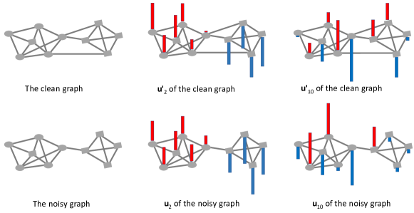
Figure 1. Graph Laplacian eigenvectors of a graph and noisy one. $\mathbf{u}_{2}$ (the eigenvector w.r.t. the second smallest eigenvalue) is stable against random noise while $\mathbf{u}_{10}$ (the eigenvector w.r.t. the largest eigenvalue) fluctuates.

An important requirement of Mask-GVAE is the ability to fast estimate stable cluster masks. While there are some neural networks proposed for computing cluster masks (Cavallari et al., 2017; Shaham et al., 2018; Chen et al., 2019; Nazi et al., 2019), they either rely on other outsourcing tools such as K-means (Shaham et al., 2018), or require as input supervised information (Chen et al., 2019). We propose an end-to-end neural network to encode cluster mask in an unsupervised manner. It differs from the above methods as (1) it uses GNN for fast computation of low eigenvectors, as GNN quickly shrinks high eigenvectors and keeps low eigenvectors (Wu et al., 2019; Li et al., 2020a); (2) it generalizes normalized cut (Shi and Malik, 2000) to work as the loss function, since the optimal solution of spectral relaxed normalized cut coincides with the low eigenvectors of normalized Laplacian (Von Luxburg, 2007).

Another challenge for Mask-GVAE is how to incorporate hard domain-specific constraints, i.e., cluster mask, into variational graph generation. In the literature, GVAE (Kusner et al., 2017) constructs parse trees based on the input graph and then uses Recurrent Neural Networks (RNNs) to encode to and decode from these parse trees. It utilizes the binary mask to delete invalid vectors. NeVAE (Samanta et al., 2019) and CGVAE (Liu et al., 2018) both leverage GNNs to generate graphs which match the statistics of the original data. They make use of a similar mask mechanism to forbid edges that violate syntactical constraint. Our model also uses the mask mechanism to generate cluster-aware graphs.

Our contributions are summarized as follows.

• We study the blind graph denoising problem. Compared with the state-of-the-art methods that mainly focus on graphs with limited sizes, our solution is the first one that does not rely on explicit eigen-decomposition and can be applied to large graphs.

• We present Mask-GVAE, the first variational generative model for blind denoising large graphs. Mask-GVAE achieves superior denoising performance to all competitors.

• We theoretically prove low eigenvectors of graph Laplacian are stable against random edge perturbations if there is a significant cluster structure, which lays the foundation of many subgraph/cluster based denoising methods.

• We evaluate Mask-GVAE on five benchmark data sets. Our method outperforms competing methods by a large margin on peak signal-to-noise ratio (PSNR) and Weisfeiler-Lehman (WL) similarity.

The remainder of this paper is organized as follows. Section 2 gives the problem definition. Section 3 describes our methodology. We provide a systematic theoretical study of the stability of low eigenvectors in Section 4. We report the experimental results in Section 5 and discuss related work in Section 6. Finally, Section 7 concludes the paper.

2. Problem definition

Consider a graph $G=(V,A,X)$ where $V=\{v_{1},v_{2},\ldots,v_{N}\}$ is the set of nodes. We use an $N\times N$ adjacency matrix $A$ to describe the connections between nodes in $V$. $A_{ij}\in\{0,1\}$ represents whether there is an undirected edge between nodes $v_{i}$ and $v_{j}$. We use $X=\{x_{1},x_{2},\ldots,x_{N}\}$ to denote the attribute values of nodes in $V$, where $x_{i}\in\mathbb{R}^{d}$ is a $d$-dimensional vector.

We assume a small portion of the given graph structure $A$ is degraded due to noise, incomplete data preprocessing, etc. The corruptions are two-fold: (1) missing edges, e.g., missing friendship links among users in a social network, and (2) irrelevant edges, e.g., incorrect interactions among proteins in a protein-protein interaction network. The problem of graph denoising is thus defined to recover a graph $\hat{G}=(V,\hat{A},X)$ from the given one $G=(V,A,X)$. In this work, we don’t consider noisy nodes and features, leaving this for future work.

Graph Laplacian regularization has been widely used as a signal prior in denoising tasks (Dong et al., 2016; Pang and Cheung, 2017). Given the adjacency matrix $A$ and the degree matrix $D$ with $D_{ii}=\sum_{j}A_{ij}$, the graph Laplacian matrix is defined as $L=D-A$. Recall $L$ is a positive semidefinite matrix, $X_{:,k}^{\top}LX_{:,k}=\frac{1}{2}\sum_{i,j=1}^{N}A_{ij}(X_{ik}-X_{jk})^{2}$ measures the sum of pairwise distances between nodes in $G$, and $X_{:,k}$ is the $k$-th column vector of $X$. In this work, we consider the recovered structure $\hat{A}$ should be coherent with respect to the features $X$. In this context, the graph denoising problem has the following objective function:

(1) $$\arg\min{}\ \ \mathcal{L}=\sum_{i<j}|A_{ij}-\hat{A}_{ij}|+\omega\Tr(X^{\top}\hat{L}X),\\$$

where the first term is a fidelity term ensuring the recovered structure $\hat{A}$ does not deviate from the observation $A$ too much, and the second term is the graph Laplacian regularizer. $\hat{L}$ is the graph Laplacian matrix for $\hat{A}$. $\omega\geq 0$ is a weighting parameter. $\Tr(\cdot)$ is defined as the sum of elements on the main diagonal of a given square matrix. In this work, we focus on blind graph denoising, i.e., we are unaware of the clean graph and the only knowledge we have is the observed graph $G=(V,A,X)$.

Our problem formulation is applicable to many real applications as illustrated below.

Application 1

In many graph-based tasks where graph structures are not readily available, one needs to construct a graph structure first (Pang and Cheung, 2017; Zeng et al., 2019; Hu et al., 2020). As an instance, the k-nearest neighbors algorithm (k-NN) is a popular graph construction method in image segmentation tasks (Felzenszwalb and Huttenlocher, 2004). One property of a graph constructed by k-NN is that each pixel (node) has a fixed number of nearest neighbors, which inevitably introduces irrelevant and missing edges. Thus, graph denoising can be used to get a denoised graph $\hat{A}$ by admitting small modifications with the observed signal prior $A$.

Application 2

Consider a knowledge graph (KG) where nodes represent entities and edges encode predicates. It is safe to assume there are some missing connections and irrelevant ones, as KGs are known for their incompleteness (Zhang et al., 2020). In this context, the task of graph denoising is to modify the observed KG such that its quality can be enhanced.

Application 3

Consider a co-authorship network as another example where a node represents an author and an edge represents the co-authorship relation between two authors. Due to the data quality issue in the input bibliographic data (e.g., name ambiguity) (Kim and Diesner, 2016), the constructed co-authorship network may contain noise in the form of irrelevant and missing edges. In this scenario, our graph denoising method can be applied to the co-authorship network to remove the noise.

We then contrast the difference between graph denoising and other related areas including adversarial learning and link prediction below.

graph denoising vs. adversarial learning

An adversarial learning method considers a specific task, e.g., node classification (Zügner et al., 2018). In this regard, there is a loss function (e.g., cross-entropy for node classification) guiding the attack and defense. Differently, we consider the general graph denoising without any task-specific loss. We thus don’t compare with the literature of adversarial learning in this work.

graph denoising vs. link prediction

While link prediction is termed as predicting whether two nodes in a network are likely to have a link (Liben-Nowell and Kleinberg, 2007), currently most methods (Liben-Nowell and Kleinberg, 2007; Zhang and Chen, 2018) focus on inferring missing links from an observed network. Differently, graph denoising considers the observed network consists of both missing links and irrelevant links. Moreover, while link prediction can take advantage of a separate trustworthy training data to learn the model, our blind setting means our model needs to denoise the structures based on the noisy input itself.

3. Methodology

Motivated by the recent advancements of discrete VAEs (Lorberbom et al., 2019) and denoising VAEs (Im et al., 2017; Chorowski et al., 2019) on images and speech, we propose to extend VAEs to the problem of denoising large discrete graphs. However, current graph VAEs still suffer from the scalability issues (Salha et al., 2019, 2020) and cannot be generalized to large-scale graph settings. As another issue, current VAEs suffer from a particular local optimum known as component collapsing (Kingma et al., 2016), meaning a good optimization of prior term results in a bad reconstruction term; if we directly attaching Eq.1 and the loss function of VAE, the situation would be worse. In this work, we present Mask-GVAE, which first decomposes a large graph into stable subgraphs and then generates smoothed subgraphs in a variational manner. Specifically, Mask-GVAE consists of two stages, one computing the cluster mask and the other generating the denoised graph.

3.1. Cluster mask

A cluster mask $C$ encodes the stable low eigenvectors of graph Laplacian. Specifically, $C\in\{0,1\}^{N\times K}$ is a binary mask, where $K$ is the number of clusters, $C_{ik}=1$ represents node $i$ belongs to cluster $k$ and $C_{ik}=0$ otherwise.

The loss function

The definition of graph cut is:

(2) $$\frac{1}{K}\sum_{k}cut(V_{k},\overline{V_{k}}),$$

where $V_{k}$ is the node set assigned to cluster $k$, $\overline{V_{k}}=V\setminus V_{k}$, $cut(V_{k},\overline{V_{k}})=\sum_{i\in V_{k},j\in\overline{V_{k}}}A_{ij}$ and it calculates the number of edges with one end point inside cluster $V_{k}$ and the other in the rest of the graph. Taking $C$ into consideration, the graph cut can be re-written as:

(3) $$\frac{1}{K}\sum_{k}(C_{:,k}^{\top}DC_{:,k}-C_{:,k}^{\top}AC_{:,k})=\frac{1}{K}\Tr(C^{\top}LC),$$

in which $D$ and $L$ are the degree and Laplacian matrices respectively. $C_{:,k}^{\top}DC_{:,k}$ stands for the number of edges with at least one end point in $V_{k}$ and $C_{:,k}^{\top}AC_{:,k}$ counts the number of edges with both end points in cluster $V_{k}$. The normalized cut (Shi and Malik, 2000; Nazi et al., 2019) thus becomes:

(4) $$\frac{1}{K}\Tr((C^{\top}LC)\oslash(C^{\top}DC)),$$

where $\oslash$ is element-wise division. Note an explicit constraint is that $C^{\top}C$ is a diagonal matrix, we thus apply a penalization term (Li et al., 2020b), which results in a differentiable unsupervised loss function:

(5) $$\mathcal{L}_{u}=\frac{1}{K}\Tr((C^{\top}LC)\oslash(C^{\top}DC))+\varphi\big{|}\big{|}\ \frac{K}{N}C^{\top}C-I_{K}\ \big{|}\big{|}_{F}^{2},$$

where $\big{|}\big{|}\cdot\big{|}\big{|}_{F}$ represents the Frobenius norm of a matrix.

The network architecture

Our architecture is similar to (Nazi et al., 2019; Li et al., 2020b) , which has two main parts: (1) node embedding, and (2) cluster assignment. In the first part, we leverage two-layer graph neural networks, e.g., GCN (Kipf and Welling, 2017), Heatts (Li et al., 2020a), to get two-hop neighborhood-aware node representations, thus those nodes that are densely connected and have similar attributes can be represented with similar node embeddings. In the second part, based on the node embeddings, we use two-layer perceptrons and softmax function to assign similar nodes to the same cluster. The output of this neural network structure is the cluster mask $C$, which is trained by minimizing the unsupervised loss $\mathcal{L}_{u}$ in Eq. 5.

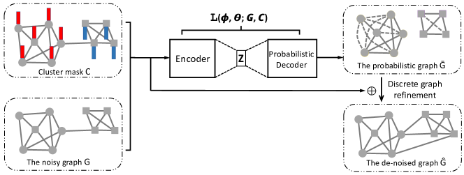
Figure 2. The proposed Mask-GVAE. It first utilizes the cluster mask $C$ and the noisy graph $G$ to learn the probabilistic de-noised graph $\bar{G}$. The learning process is conditioned on $C$ as cluster results are robust against random noise (Proposition 4.1). With the optimum of the learning process, it then draws discrete graph $\hat{G}$ at test time to meet the fidelity constraint.

3.2. Denoised graph generation

In this subsection, we describe our method (illustrated in Figure 2) which produces a denoised graph $\hat{A}$ that is conditioned on the cluster mask $C$ and meets the fidelity constraint. As discussed, we use a latent variable model parameterized by neural networks to generate the graph $\hat{G}$. Specifically, we focus on learning a parameterized distribution over the graph $G$ and the cluster mask $C$ as follows:

(6) $$P(\hat{A}|G,C)=\int q_{\phi}(Z|G,C)p_{\theta}(\hat{A}|G,C,Z)dZ,$$

where $q_{\phi}(Z|G,C)$ is the encoder and $p_{\theta}(\hat{A}|G,C,Z)$ is the decoder. While the encoder is straightforward and we can use the corresponding encoders in existing work (Kipf and Welling, 2016), the decoder is hard due to the following two factors:

• Discrete decoding: Generating discrete graphs is challenging.

• Cluster awareness: Existing graph generation methods cannot explicitly incorporate cluster information.

To satisfy the discrete decoding, we decouple the decoder into two steps: (1) probabilistic graph decoder, which produces a probabilistic graph $\bar{A}$ in training, and (2) discrete graph refinement, in which we sample a discrete graph $\hat{A}$ in testing based on the prior knowledge $G$ and $\bar{A}$. To address the cluster awareness, we propose to directly incorporate cluster information into the learning process by using the mask (Kusner et al., 2017) mechanism, which powers the model with the ability to generate denoised graph with smoothed subgraphs.

Graph encoder

We follow VGAE (Kipf and Welling, 2016) by using the mean field approximation to define the variational family:

(7) $$q_{\phi}(Z|G,C)=\prod_{i=1}^{N}q_{\phi_{i}}(z_{i}|A,X),$$

where $q_{\phi_{i}}(z_{i}|A,X)$ is the predefined prior distribution, namely, isotropic Gaussian with diagonal covariance. The parameters for the variational marginals $q_{\phi_{i}}(z_{i}|A,X)$ are specified by a two-layer GNN (Kipf and Welling, 2017; Li et al., 2020a):

(8) $$\mu,\sigma=\text{GNN}_{\phi}(A,X),$$

where $\mu$ and $\sigma$ are the vector of means and standard deviations for the variational marginals $\{q_{\phi_{i}}(z_{i}|A,X)\}_{i=1}^{N}$. $\phi=\{\phi_{i}\}_{i=1}^{N}$ is the parameter set for encoding.

Probabilistic graph decoder

We first compute the edge probability:

(9) $$p_{\theta}(\bar{A}_{ij}|G,C,Z)=\bar{A}_{ij}=\text{sigmoid}(W_{a1}\text{ReLU}(W_{a2}E_{ij})),$$

where $E_{ij}=[Z_{i}|X_{i}]\odot[Z_{j}|X_{j}]$, $Z_{i}|X_{i}$ is a concatenation of $Z_{i}$ and $X_{i}$, $\odot$ represents element-wise multiplication. Intuitively we compute the edge probability by two-layer perceptrons and sigmoid function.

The loss function

We approximate $p(\bar{A}|G,C,Z)$ by:

(10) $$\begin{split}p(\bar{A}|G,C,Z)=\prod_{(CC^{\top})_{ij}=1}\bar{A}_{ij}\prod_{(CC^{\top})_{ij}=0}(1-\bar{A}_{ij}),\end{split}$$

where $(CC^{\top})_{ij}=1$ denotes node $i$ and node $j$ are in the same cluster and $(CC^{\top})_{ij}=0$ otherwise. When the number of clusters $K$ is large, it is beneficial to re-scale both $CC^{\top}_{ij}=1$ and $CC^{\top}_{ij}=0$ within $A_{ij}=1$ .

(11) $$S=CC^{\top}\odot A,$$

where $S_{ij}=1$ denotes node $i$ and node $j$ are adjacent and in the same cluster w.r.t. the cluster mask $C$. With $S$, $(A-S)$ can be used to denote the inter-cluster connections.

The overall loss for Mask-GVAE is:

(12) $$\begin{split}\mathcal{L}(\phi,\theta;G,C)=\mathcal{L}_{prior}-\mathbb{E}_{q_{\phi}(Z/G,C)}(\log p(\bar{A}|G,C,Z)),\end{split}$$

where $\mathcal{L}_{prior}=\text{KL}(q(Z|G,C)||p(Z))$ is the prior loss with $p(Z)=\prod_{i=1}^{N}P(z_{i})=\prod_{i=1}^{N}\mathcal{N}(z_{i}|0,I)$. Intuitively, Eq. 12 takes into consideration both the objective function in Eq. 1 and cluster structures.

Discrete graph refinement

At testing time, we draw discrete samples from the probabilistic graph $\bar{G}=(V,\bar{A},X)$. To ensure the de-noised graph $\hat{A}$ does not deviate from the observation $A$ too much, we set a budget $\Delta$ to measure their difference. We split the budget into two parts, $\Delta/2$ for adding edges, and $\Delta/2$ for deleting edges. The refinement strategy is simply sampling without replacement from the formulated Category distributions.

To delete edges, we restrict ourselves to existing inter-cluster connections $(A-S)_{ij}=1$.

$$E_{ij}^{-}=\frac{\exp{(1-\bar{A}_{ij})}}{\sum\exp{(1-\bar{A}_{ij})}}\ \ \ \ if\ \ \ \ (A-S)_{ij}=1.$$

We sample without replacement $\Delta/2$ edges according to their probabilities $E_{ij}^{-}$. The sampled edge set is then deleted from the original graph structure $A$. To add edges, we are allowed to add connections for intra-cluster nodes $(CC^{\top}-A)_{ij}=1$.

$$E_{ij}^{+}=\frac{\exp{\bar{A}_{ij}}}{\sum\exp{\bar{A}_{ij}}}\ \ \ \ if\ \ \ \ (CC^{\top}-A)_{ij}=1.$$

We sample $\Delta/2$ edges according to their probabilities $E_{ij}^{+}$. The sampled edge set is added into the original graph structure $A$. With this strategy, we can generate the final denoised graph structure $\hat{A}$.

Connection between Mask-GVAE and Eq. 1

The first term of Eq. 1 is used to ensure the proximity between the input graph $A$ and the denoised graph $\hat{A}$, which is achieved in Mask-GVAE by the reconstruction capacity of VAEs and the discrete budget in the sampling stage. Next, we illustrate the connection between the graph Laplacian term in Eq. 1 and Mask-GVAE. We can re-write the graph Laplacian regularization when $d=1$ as:

(13) $$X^{\top}LX_{d=1}=\frac{1}{2}(\underbrace{\sum_{S_{ij}=1}(X_{i}-X_{j})^{2}}_{intra-cluster}+\underbrace{\sum_{(A-S)_{ij}=1}(X_{i}-X_{j})^{2}}_{inter-cluster}),$$

By decomposing the Laplacian regularization into these two terms, we focus on intra/inter-cluster connections when adding/deleting edges. As attributed graph clustering aims to discover groups of nodes in a graph such that the intra-group nodes are not only more similar but also more densely connected than the inter-group ones (Wang et al., 2015), this heuristic contributes to the overall optimization of the graph Laplacian term.

3.3. The Proposed Training Method

Our solution consists of a cluster mask module $f(\cdot)$ and a denoised graph generation module $g(\cdot)$. As the error signals of the denoised graph generation module are obtained from the cluster mask module and the cluster mask module needs the denoised graphs as inputs for robust cluster results, we design an iterative framework, to alternate between minimizing the loss of both $g(\cdot)$ and $f(\cdot)$. We refer to Algorithm 1 for details of the training procedure.

We denote the parameters of the cluster mask module $f(\cdot)$ as $\mathcal{W}_{f}$ and the parameters of the denoised graph generation module $g(\cdot)$ as $\mathcal{W}_{g}$. At the beginning of Algorithm 1, we use the cluster mask module $f(\cdot)$ to get the initial cluster results. We then exploit the denoised graph generator $g(\cdot)$ so as to get a denoised graph $\hat{G}$ (line 4). Based on that, we utilize the idea of randomized smoothing (Jia et al., 2020; Cohen et al., 2019) and feed both $G$ and $\hat{G}$ into the cluster mask module $f(\cdot)$ to compute $\mathcal{L}_{u}$ (line 7). With the optimum of $f(\cdot)$, we get the robust cluster mask $C$ to power the learning process of $g(\cdot)$ (line 9).

Input: $G$, $K$.

Output: $\hat{G}$.

1 Initial: parameters $\mathcal{W}_{g}$,$\mathcal{W}_{f}$;

2repeat

3       $C\leftarrow$ $f(G,K)$;

4       $\hat{G}\leftarrow$ $g(G,C)$;

5       $\mathcal{L}_{prior}\leftarrow\text{KL}(q(Z|G,C)||p(Z))$;

6       $\mathcal{L}(\phi,\theta;G,C)\leftarrow\mathcal{L}_{prior}-\mathbb{E}_{q_{\phi}(Z/G,C)}(\log p(\bar{A}|G,C,Z))$;

7       $\mathcal{L}_{u}\leftarrow f(\{G,\hat{G}\})$;

8       // Update parameters according to gradients

9      $\mathcal{W}_{g}\leftarrow^{+}-\bigtriangledown_{\mathcal{W}_{g}}\mathcal{L}(\phi,\theta;G,C)$;

10       $\mathcal{W}_{f}\leftarrow^{+}-\bigtriangledown_{\mathcal{W}_{f}}\mathcal{L}_{u}$;

11      

12until deadline;

Algorithm 1 Training the model

3.4. Complexity Analysis

We analyze the computational complexity of our proposed method. The intensive parts of Mask-GVAE contain the computation of Eq. 5 and Eq. 12. Aside from this, the convolution operation takes $O(|E|dh)$ (Kipf and Welling, 2017) for one input graph instance with $|E|$ edges where $h$ is the number of feature maps of the weight matrix.

Regarding Eq. 5, the core is to compute the matrices $(C^{\top}LC)$ and $(C^{\top}DC)$. Using sparse-dense matrix multiplications, the complexity is $O(|E|K^{2})$. For Eq. 12, the intensive part is the topology reconstruction term. As the optimization is conditioned on existing edges, the complexity is $O(|E|)$. Thus, it leads to the complexity of $O(|E|K^{2}+|E|dh)$ for one input graph instance.

We compare with VGAE (Kipf and Welling, 2016) and one of our baseline DOMINANT (Ding et al., 2019), whose operations require several convolution layers with $O(|E|dh)$ and topology reconstruction term on all possible node pairs $O(N^{2})$. Thus, the complexity of VGAE and DOMINANT is $O(N^{2}+|E|dh)$. As observed in the experiments, usually we have $|E|K^{2}\leq N^{2}$ for large graphs, e.g., Citeseer, Pubmed, Wiki, Reddit. When compared with NE (Wang et al., 2018) and ND (Feizi et al., 2013), our solution wins as both NE and ND rely on explicit eigen-decomposition.

4. Assumption analysis

The stability of cluster mask under random noise is vital for Mask-GVAE, and that stability is dominated by the stability of low eigenvectors of graph Laplacian (Von Luxburg, 2007). In this part, we initiate a systematic study of the stability of low eigenvectors, using the notion of average sensitivity (Varma and Yoshida, 2019), which is the expected size of the symmetric difference of the output low eigenvectors before and after we randomly remove a few edges. Let the clean graph be $G^{\prime}=(V,A^{\prime},X)$, the degree matrix be $D^{\prime}$ and the clean Laplacian matrix be $L^{\prime}=D^{\prime}-A^{\prime}$. We denote the $i$-th smallest eigenvalue of $L^{\prime}$ as $\lambda^{\prime}_{i}$, and the corresponding eigenvector as $\mathbf{u^{\prime}}_{i}$. We consider the noisy graph $G=(V,A,X)$ is generated from the clean one $G^{\prime}$ by the following procedure: for each edge $(i,j)$ in $G^{\prime}$, remove it with probability $q$ independently. Following (Huang et al., 2009), we analyze the bi-partition of the graph data, as a larger number of clusters can be found by applying the bi-partition algorithm recursively.

Assumption 4.1.

Let the node degrees of the clean graph be $\sum\limits_{i=1}^{N}d{{}^{\prime}}_{i}^{2}=N^{\chi}$ and the number of edges be $m^{\prime}=N^{\varphi}$, the following properties hold.

1. $\exists\epsilon\geq 2,s.t.,\frac{2\epsilon}{\epsilon-1}\lambda^{\prime}_{2}<\lambda^{\prime}_{3}$ and $\lambda^{\prime}_{3}\geq\max(\frac{25}{2}\epsilon q\lambda^{\prime}_{N},\frac{3}{2}\epsilon\log N)$.

2. $q\leq\frac{\lambda^{\prime}_{2}}{\kappa N^{\beta}}$ and $\beta\geq\frac{1}{2}\max(\chi,\varphi)$ with $\kappa>1$.

Assumption 4.1.1 implies the graph has at most one outstanding sparse cut by the higher-order Cheeger inequality (Lee et al., 2014; Peng and Yoshida, 2020). It has been discussed that the eigenspaces of Laplacian with such a large eigengap are stable against edge noise (Von Luxburg, 2007). Assumption 4.1.2 indicates the probability of edge noise is small w.r.t. the number of nodes. To better understand Assumption 4.1, let us consider the example in Figure 1. It is easy to check $\chi=2.32$, $\varphi=1.3$, $\lambda^{\prime}_{2}=0.78$, $\lambda^{\prime}_{3}=3.28$ and $\lambda^{\prime}_{N}=6.96$. Let $q=0.01$, then we can get $\beta=1.16$ and $\kappa=5.4$.

Table 1. Statistics of graphs used in graph clustering

Data	Nodes	Edges	Class	features
Citeseer	3,327	4,732	6	3,703
Pubmed	19,717	44,338	3	500
Wiki	2,405	17,981	17	4,973

Denote $\mathbb{E}[\sin(\angle(\mathbf{u^{\prime}}_{2},\mathbf{u}_{2}))]$ as the expected $\sin(\angle(\cdot,\cdot))$ for the angle between $\mathbf{u^{\prime}}_{2}$ and $\mathbf{u}_{2}$, then the following proposition holds.

Proposition 4.1.

Under Assumption 4.1, $\mathbb{E}[\sin(\angle(\mathbf{u^{\prime}}_{2},\mathbf{u}_{2}))]$ under random noise satisfies $\mathbb{E}[\sin(\angle(\mathbf{u^{\prime}}_{2},\mathbf{u}_{2}))]\leq\frac{1}{\kappa}$.

Please refer to Appendix A for the proof. For the example in Figure 1, we can check $\mathbb{E}[\sin(\angle(\mathbf{u^{\prime}}_{2},\mathbf{u}_{2}))]\approx 0.07\leq 1/5.4$.

5. Experiments

We first validate the effectiveness of our graph clustering algorithm. Then we evaluate Mask-GVAE on blind graph denoising tasks.

5.1. Graph clustering

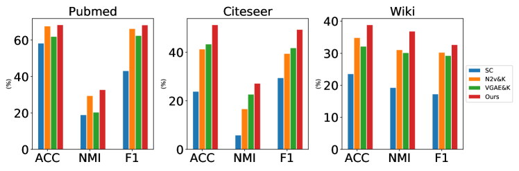
Figure 3. Graph clustering performance comparison of different methods

Data and baselines

We use three benchmark data sets, i.e., Pubmed, Citeseer (Sen et al., 2008) and Wiki (Yang et al., 2015). Statistics of the data sets can be found in Table 1. As baselines, we compare against (1) Spectral Clustering (SC) (Von Luxburg, 2007), which only takes the node adjacency matrix as affinity matrix; (2) Node2vec (Grover and Leskovec, 2016) + Kmeans (N2v&K), which first uses Node2vec to derive node embeddings and then utilizes K-means to generate cluster results; and (3) VGAE (Kipf and Welling, 2016) + Kmeans (VGAE&K).

Setup

For our method, we let the output dimension of the second-layer perceptrons equal to the number of clusters. We use the same network architecture through all the experiments. Our implementation is based on Tensorflow. We train the model using full batch based Adam optimizer with exponential decay. We set $\varphi=0.01$. The output dimension of the first-layer GNN is 32. The best variants of GNN are chosen from GCN (Kipf and Welling, 2017) and Heatts (Li et al., 2020a). In addition, we use a dropout rate of 0.3 for all layers. The initial learning rate is 0.01. We leverage node class labels as the ground truth for graph clustering.

Results

The clustering accuracy (ACC), normalized mutual information (NMI) and macro F1 score (F1) are shown in Figure 3. Our method outperforms the competitors on all data sets. As ours does not rely on K-means to derive cluster memberships, this cluster performance indicates the effectiveness of our framework on graph clustering tasks.

5.2. Graph denoising

Baselines

We use the following approaches as our baselines:

• DOMINANT (Ding et al., 2019), a graph neural network that performs anomaly detection on attributed graph. It computes the degree of anomaly by the distance of recovered features/edges and the input features/edges. In this work, we consider the top anomaly edges as noisy edges and remove them from the input graphs.

• NE (Wang et al., 2018), a blind graph denoising algorithm that recovers the graph structure based on diffusion algorithms. It is designed to remove irrelevant edges in biological networks. It relies on explicit eigen-decomposition and cannot be applied to large graphs.

• ND (Feizi et al., 2013), a blind graph denoising algorithm that solves an inverse diffusion process to remove the transitive edges. It also relies on explicit eigen-decomposition and cannot be applied to large graphs.

• E-Net (Xu et al., 2020), a non-blind graph enhancement neural network that draws inspirations from link prediction method (Zhang and Chen, 2018). For a fair comparison, we replace the supervision (clean graphs) used in E-Net with the noisy version.

• Our-ablation, an ablation of our framework that does not utilize cluster mask. It resembles VGAE (Kipf and Welling, 2016) with two differences: (1) we use a multi-layer perceptron in decoders while VGAE uses a non-parameterized version, and (2) we replace GCN (Kipf and Welling, 2017) with Heatts (Li et al., 2020a).

Metrics

We follow image denoising (Pang and Cheung, 2017; Zeng et al., 2019) to use peak signal-to-noise ratio (PSNR) when the clean graph $G^{\prime}=(V,A^{\prime},X)$ is known.

(14) $$\text{MSE}=\frac{\sum_{i}^{N}\sum_{j}^{i}(A^{\prime}_{ij}-\hat{A}_{ij})^{2}}{N(N-1)}.$$

PSNR is then defined as:

(15) $$\text{PSNR}=10\log(\frac{1}{\text{MSE}}).$$

As for the structural similarity, we leverage Weisfeiler-Lehman Graph Kernels (Shervashidze et al., 2011).

(16) $$WL=\frac{\langle\phi(\hat{A}),\phi(A^{\prime})\rangle}{\sqrt{\langle\phi(\hat{A}),\phi(\hat{A})\rangle\langle\phi(A^{\prime}),\phi(A^{\prime})\rangle}},$$

where $\langle\cdot,\cdot\rangle$ denotes dot product, $\phi(\cdot)$ represents a vector derived by Weisfeiler-Lehman Graph Kernels.

For all metrics, a greater value denotes a better performance.

Table 2. Blind denoising performance comparison of different methods on benchmarks

Datasets	IMDB-BIN		IMDB-MULTI		REDDIT-BIN		MUTAG		PTC-MR
(No. Graphs)	1000		1500		2000		188		344
(Avg. Nodes)	19.8		13.0		508.5		17.9		14.3
(Avg. Edges)	193.1		65.9		497.8		19.8		14.7
Metrics	PSNR	WL	PSNR	WL	PSNR	WL	PSNR	WL	PSNR	WL
DOMINANT (Ding et al., 2019)	$50.81\pm 0.33$	$19.79\pm 0.41\%$	$49.29\pm 0.65$	$54.33\pm 0.81\%$	$74.97\pm 1.17$	$21.88\pm 0.69\%$	$55.09\pm 0.47$	$25.74\pm 1.10\%$	$42.21\pm 0.51$	$24.88\pm 0.45\%$
ND (Feizi et al., 2013)	$47.08\pm 0.11$	$22.47\pm 0.14\%$	$53.22\pm 0.05$	$55.73\pm 0.03\%$	-	-	$43.00\pm 0.18$	$9.37\pm 0.22\%$	$38.12\pm 0.27$	$22.84\pm 0.30\%$
NE (Wang et al., 2018)	$51.81\pm 0.17$	$25.87\pm 0.09\%$	$55.40\pm 0.21$	$57.30\pm 0.14\%$	-	-	$54.30\pm 0.22$	$25.65\pm 0.18\%$	$47.92\pm 0.05$	$22.85\pm 0.11\%$
E-Net (Xu et al., 2020)	$49.18\pm 0.97$	$18.38\pm 1.15\%$	$55.57\pm 1.01$	$56.14\pm 1.62\%$	$87.48\pm 1.33$	$22.54\pm 1.07\%$	$52.42\pm 1.58$	$30.53\pm 1.42\%$	$50.73\pm 1.66$	$34.51\pm 0.92\%$
Our-ablation	$52.75\pm 0.48$	$21.47\pm 0.33\%$	$55.82\pm 0.59$	$57.85\pm 0.55\%$	$75.35\pm 1.10$	$23.44\pm 0.96\%$	$55.76\pm 0.68$	$27.90\pm 1.12\%$	$47.52\pm 0.44$	$33.20\pm 0.83\%$
Mask-GVAE	$\bf{55.74\pm 0.51}$	$\bf{26.41\pm 0.49\%}$	$\bf{56.86\pm 0.66}$	$\bf{58.25\pm 0.74\%}$	$\bf{98.41\pm 0.71}$	$\bf{25.32\pm 0.56\%}$	$\bf{56.72\pm 0.31}$	$\bf{36.84\pm 0.22\%}$	$\bf{52.06\pm 0.56}$	$\bf{38.73\pm 0.36\%}$

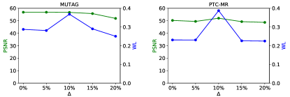
Figure 4. Influence of the estimated noise $\Delta$ on the denoising performance of MUTAG(left) and PTC-MR(right)

Data

We use five graph classification benchmarks: IMDB-Binary and IMDB-Multi (Yanardag and Vishwanathan, 2015) connecting actors/actresses based on movie appearance, Reddit-Binary (Yanardag and Vishwanathan, 2015) connecting users through responses in Reddit online discussion, MUTAG (Kriege and Mutzel, 2012) containing mutagenic compound, PTC (Kriege and Mutzel, 2012) containing compounds tested for carcinogenicit, as the clean graphs. For each $A^{\prime}$, we add noise to edges to produce $A$ by the following methods: (1) randomly adding 10% nonexistent edges, (2) randomly removing 10% edges with respect to the existing edges in $A^{\prime}$, as adopted in E-Net (Xu et al., 2020). We refer to Table 2 for the detailed information about the obtained noisy graphs.

Setup

For Mask-GVAE, we adopt the same settings as in the experiment of graph clustering except that we use Bayesian Information Criterion (BIC) to decide the optimal number of clusters. For all methods, we denoise the given graphs with the same budget, i.e., we add 10% edges to recover missing edges and remove 10% edges to delete irrelevant edges, based on the intermediate probabilistic graphs.

Table 3. Running time (in seconds) comparison of different methods

Data sets	IMDB-MULTI	REDDIT-BIN	PTC-MR
DOMINANT	73	1895	11
ND	41	-	6
NE	43	-	14
E-Net	216	2114	19
Mask-GVAE	79	1043	21

Results

Table 2 lists the experimental results on the five data sets respectively. We analyse the results from the following two perspectives.

Scalability: Both ND and NE suffer from a long run time and take more than 1 day on the larger data set Reddit-Binary, as they both rely on explicit eigen-decomposition. On the contrary, E-Net and our method can take advantage of GNN and avoid explicit eigen-decomposition, which makes the algorithms scalable to very large networks.

Performance: Among all approaches, Mask-GVAE achieves the best performance on all data sets in terms of the two measures PSNR and WL similarity. It also beats Our-ablation, which shows the effectiveness of cluster mask.

Running time

Table 3 lists the running time on the three selected data sets. As can be seen, on small-sized graphs like PTC-MR, Mask-GVAE requires longer time as it needs to compute the cluster mask. On medium-sized graphs like IMDB-MULTI, the running time of Mask-GVAE is comparable to that of DOMINANT and NE/ND. On large-sized graphs like REDDIT-BIN, Mask-GVAE uses less time compared with all baselines, as the optimization of denoised graph generation in Mask-GVAE is conditioned on the observed edges.

Sensitivity

We test the sensitivity of Mask-GVAE to the degree of noise and modularity (Newman, 2006) in given graphs. We target random cluster graphs (Newman, 2009) and generate 200 synthetic graphs with an average of 100 nodes. We set the degree of noise to 10%, 20% and 30%. We control the modularity to be 0.05 (weak cluster structure) and 0.35 (strong cluster structure). Table 4 lists the results. As can be seen, our solution consistently outperforms baselines in most cases, regardless of the degree of noise and cluster structure. In addition, we observe most methods perform better in PSNR on strong clustered graphs (modularity = 0.35), which shows the importance of clusters in current denoising approaches.

Estimating the degree of noise

Estimating the degree of noise for the given inputs is still an open problem (Guo et al., 2019). In this work, we use budget $\Delta$ to represent our estimation on the degree of noise in the given graphs. In this part, we evaluate how the budget $\Delta$ affects the denoising performance. Taking MUTAG/PTC-MR with 10% noise as an example, we vary $\Delta$ from 0% to 20% and plot the corresponding denoising performance in Figure 4. As we increase $\Delta$, the curve of PSNR is quite flat, indicating our model is robust to the estimated noise on PSNR. As for WL, it first increases then drops, meaning that an appropriate noise estimation is essential for the performance of our model on structural similarity.

Table 4. Performance comparison of different methods on the random cluster graphs

Degree of noise	10%				20%				30%
Modularity	0.05		0.35		0.05		0.35		0.05		0.35
-	PSNR	WL	PSNR	WL	PSNR	WL	PSNR	WL	PSNR	WL	PSNR	WL
DOMINANT	74.01	48.57%	75.54	48.57%	71.05	37.88%	72.64	34.51%	70.39	35.23%	72.59	34.50%
ND	72.70	48.19%	75.67	46.60%	71.30	27.20%	73.74	28.73%	70.37	18.01%	71.98	17.20%
NE	74.48	46.67%	76.82	44.24%	71.98	35.06%	73.66	33.66%	70.33	27.67%	72.10	28.07%
E-Net	75.91	48.17%	77.58	47.88%	72.24	38.94%	74.09	36.47%	70.36	34.99%	72.51	33.09%
Mask-GVAE	76.32	48.94%	78.01	50.07%	72.73	48.37%	74.66	36.82%	70.49	36.14%	72.68	35.99%

Visualization

We target Citeseer and add 30% noise. In Figure 5, we derive node embeddings before/after Mask-GVAE by Node2vec (Grover and Leskovec, 2016) and project the embeddings into a two-dimensional space with t-SNE, in which different colors denote different classes. For noised Citeseer, nodes of different classes are mixed up, as reflected by the geometric distances between different colors. Mask-GVAE can make a distinct difference between classes.

Case study

To have a better understanding of how Mask-GVAE works, we target a subgraph of co-authorship network which consists of 11 scholars in the area of Data Base (DB) and Data Mining (DM). The subgraph is based on Google Scholar and constructed as follows: (1) for each scholar, we use a one-hot representation with 300 dimensions encoding his/her research keywords, and (2) we construct an adjacency matrix $A$ by denoting $A_{ij}=1$ and $A_{ji}=1$ if the two scholars have co-authored papers. We apply Mask-GVAE on this subgraph and set $K=2$ and $\Delta=1$ to remove irrelevant edges. As can be seen from Figure 6, Mask-GVAE identifies the connection between “Wenjie Zhang” and “Wei Wang (UCLA)” as the noisy edge. We further notice that the noisy edge is constructed based on paper (Li et al., 2019b), which is actually co-authored by “Wenjie Zhang” and “Wei Wang (UNSW)”. One possible explanation is that Google Scholar fails to distinguish “Wei Wang (UNSW)” and “Wei Wang (UCLA)”, as a result the paper (Li et al., 2019b) appears on the Google Scholar page of “Wei Wang (UCLA)” mistakenly.

As a comparison, when we apply ND, NE and E-Net on this subgraph, only NE can pick up the noisy connection, while ND and E-Net cannot. One possibility is Mask-GVAE and NE are designed to keep the cluster structure. But ND targets “Jeffery Xu Yu” and “Wei Wang (UCLA)” and E-Net targets “Jeffery Xu Yu” and “Jiawei Han”, both of which are true connections.

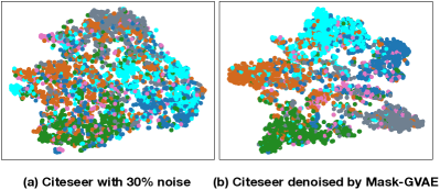
Figure 5. Two-dimensional visualization of node embeddings before and after the denoising of Mask-GVAE on Citeseer.

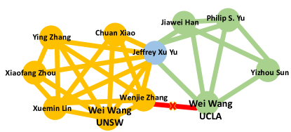
Figure 6. A case to show how Mask-GVAE denoises graphs

6. Related work

Graph Laplacian in denoising tasks. Several studies have utilized graph Laplacian in various denoising tasks, including image denoising (Pang and Cheung, 2017; Zeng et al., 2019), signal denoising (Dong et al., 2016), and 3D point cloud denoising (Hu et al., 2020). As graph structures are not readily available in these domains, these studies differ in how they construct graph structures, i.e., structures are only created as an auxiliary source to recover a high quality image/signal/3D point cloud. Only recently, E-Net (Xu et al., 2020) has proposed to adopt Graph Laplacian regularization in non-blind graph denoising tasks, in order to restore a denoised graph with global smoothing and sparsity.

Graph denoising. Although there have been many studies on image denoising, graph denoising has been studied less, in particular, the study of blind denoising large discrete graphs is still lacking. It is worth noting the study of signal denoising on graphs (Chen et al., 2014; Padilla et al., 2017) is different from the study of graph structure denoising. When it comes to structure denoising, ND (Feizi et al., 2013) formulates the problem as the inverse of network convolution, and introduces an algorithm that removes the combined effect of all indirect paths by exploiting eigen-decomposition. NE (Wang et al., 2018) recovers the graph structure based on diffusion algorithms and follows the intuition that nodes connected by high-weight paths are more likely to have direct edges. Low-rank estimation (Hsieh et al., 2012) and sparse matrix estimation (Richard et al., 2012) assume the given graph is incomplete and noisy, thus they aim to recover the structure with the property of low-rank/sparsity. (Morris and Frey, 2004) infers the hidden graph structures based on the heuristic that a set of hidden, constituent subgraphs are combined to generate the observed graph. Inspired by link prediction (Zhang and Chen, 2018), E-Net (Xu et al., 2020) enhances the quality of graph structure via exploiting subgraph characteristics and GNNs. Moreover, E-NET requires supervision of the clean graphs, which is different from our blind setting.

Utilization of substructure. It is a common practice to utilize certain substructures (i.e., clusters or subgraphs) in denoising tasks (Morris and Frey, 2004; Xu et al., 2020; Feizi et al., 2013) or other related areas (Zhang and Chen, 2018; Chiang et al., 2019). The underlying ideas can be generally classified into two groups. The first group is related to scalability, i.e., substructures make the algorithms scalable to very large networks. Representative works include ND (Feizi et al., 2013), E-Net (Xu et al., 2020), Cluster-GCN (Chiang et al., 2019). The second group considers substructures can provide meaningful context for the tasks at hand. For example, SEAL (Zhang and Chen, 2018) shows that local subgraphs reserve rich information related to link existence. However, all these methods are heuristic methods and shed little light on when these substructure based ideas fail. In this work, we prove that in order to make substructure heuristics work, the given graph should have a distinct cluster structure. Moreover, it is the robustness of low eigenvectors in graph Laplacian matrix that lays the foundation of these heuristics.

Discrete graph generation. Directly generating discrete graph with gradient descent methods is intractable. In this regard, several efforts have been made to bypass the difficulty. (Bello et al., 2017) learns a policy network with reinforcement learning, (Jang et al., 2016) approximates the discrete data by Gumbel distribution, (Simonovsky and Komodakis, 2018) circumvents the problem by formulating the loss on a probabilistic graph and drawing discrete graphs thereafter, which we follow in this work.

7. Conclusion

In this paper, we present Mask-GVAE, the first variational generative model for blind denoising large discrete graphs. Given the huge search space of selecting proper candidates, we decompose the graph into several subgraphs and generate smoothed clusters in a variational manner, which is based on the assumption that low eigenvectors are robust against random noise. The effectiveness of Mask-GVAE is validated on five graph benchmarks, with a significant improvement on PSNR and WL similarity.

Appendix A Proof of Proposition 4.1

Lemma A.1.

If Assumption 4.1 holds, then $P(\lambda_{3}\geq(1-\frac{1}{\epsilon})\lambda^{\prime}_{3})\geq 1-N^{-\frac{1}{8}}$.

We first prove lemma A.1. Let $E$ be the set of edges of $G^{\prime}$, $F$ be the set of edges removed from $E$, $E_{e}=E_{ii}+E_{jj}-E_{ij}-E_{ji}$, $E_{ij}$ is the matrix with 1 for position $(i,j)$ and 0 for others, and $E_{F}=\sum_{e\in F}E_{e}$, if $(i,j)\in E$. Let $X_{e}$ be an indicator random variable of the event that $e\in F$. Thus, $E_{F}=\sum_{e\in E}=X_{e}E_{e}$, $E_{F}$ is the Laplacian matrix of the induced graph $F$. It is easy to get $P[X_{e}=1]=q$, $\mathbb{E}[E_{F}]=qL^{\prime}$. Let $\mu=\lambda_{max}(\mathbb{E}[E_{F}])=q\lambda^{\prime}_{N}$. Furthermore, note that $0\leq\lambda(X_{e}E_{e})\leq\lambda_{max}(X_{e}E_{e})\leq 2$. By the matrix Chernoff bound in Peng and Yoshida (Peng and Yoshida, 2020), for any $s>0$, we have

$$P(\lambda_{max}(E_{F})\geq(1+s)\mu)\leq N\Big{(}\frac{\exp(s)}{(1+s)^{1+s}}\Big{)}^{\frac{1}{2}\mu}.$$

Set $1+s=\frac{25}{2},(1+s)\mu=\frac{3}{2}\log N$, then $P(\lambda_{max}(E_{F})\geq(1+s)\mu)\leq N^{-\frac{1}{8}}$. Thus with probability at least $1-N^{-\frac{1}{8}}$, $\lambda_{max}(E_{F})\leq\max(\frac{25}{2}\mu,\frac{3}{2}\log N)=\max(\frac{25}{2}q\lambda^{\prime}_{N},\frac{3}{2}\log N)\leq\frac{\lambda^{\prime}_{3}}{\epsilon}$ holds. Due to the fact that $\lambda_{3}\geq\lambda^{\prime}_{3}-\lambda_{max}(E_{F})$, $P(\lambda_{3}\geq(1-\frac{1}{\epsilon})\lambda^{\prime}_{3})\geq 1-N^{-\frac{1}{8}}$ holds.

With lemma A.1, we prove Proposition 4.1 based on the well-known Davis-Kahan perturbation theorem.

It is easy to show that $\mathbb{E}[\|L-L^{\prime}\|_{F}]=q\|L^{\prime}\|_{F}$.

Define $\delta=\min\{|\lambda_{j}-\lambda^{\prime}_{2}|,j\neq 2\}$, we can get the following bound according to Davis-Kahan theorem,

$$\mathbb{E}[\sin(\angle(\mathbf{u}_{2},\mathbf{u^{\prime}}_{2}))]\leq\mathbb{E}[\frac{1}{\delta}\|L-L^{\prime}\|_{F}]=\frac{1}{\delta}(q\|L^{\prime}\|_{F}).$$

Easy to check $\|L^{\prime}\|_{F}^{2}=O(\max(N^{\chi},N^{\varphi}))$.

By Lemma A.1, we have $P(\lambda_{3}\geq(1-\frac{1}{\epsilon})\lambda^{\prime}_{3})\geq 1-N^{-\frac{1}{8}}$. Note that if $\frac{2\epsilon}{\epsilon-1}\lambda^{\prime}_{2}<\lambda^{\prime}_{3}$, then $\delta=\lambda^{\prime}_{2}$, thus

if $\beta>\frac{1}{2}\max(\chi,\varphi)$, then $\mathbb{E}[\sin(\angle(\mathbf{u}_{2},\mathbf{u^{\prime}}_{2}))]\rightarrow 0$.

if $\beta=\frac{1}{2}\max(\chi,\varphi)$, then $\mathbb{E}[\sin(\angle(\mathbf{u}_{2},\mathbf{u^{\prime}}_{2}))]\leq\frac{1}{\kappa}$.

References

- (1)
- Ahn et al. (2010) Yong-Yeol Ahn, James P Bagrow, and Sune Lehmann. 2010. Link communities reveal multiscale complexity in networks. Nature 466, 7307 (2010), 761–764.
- Bello et al. (2017) Irwan Bello, Hieu Pham, Quoc V Le, Mohammad Norouzi, and Samy Bengio. 2017. Neural combinatorial optimization with reinforcement learning. International Conference on Learning Representations (ICLR) (2017).
- Cavallari et al. (2017) Sandro Cavallari, Vincent W Zheng, Hongyun Cai, Kevin Chen-Chuan Chang, and Erik Cambria. 2017. Learning community embedding with community detection and node embedding on graphs. In Proceedings of the 2017 ACM on Conference on Information and Knowledge Management (CIKM). ACM, 377–386.
- Chen et al. (2014) Siheng Chen, Aliaksei Sandryhaila, José MF Moura, and Jelena Kovacevic. 2014. Signal denoising on graphs via graph filtering. In 2014 IEEE Global Conference on Signal and Information Processing (GlobalSIP). IEEE, 872–876.
- Chen et al. (2019) Zhengdao Chen, Xiang Li, and Joan Bruna. 2019. Supervised community detection with line graph neural networks. International Conference on Learning Representations (ICLR) (2019).
- Chiang et al. (2019) Wei-Lin Chiang, Xuanqing Liu, Si Si, Yang Li, Samy Bengio, and Cho-Jui Hsieh. 2019. Cluster-GCN: An efficient algorithm for training deep and large graph convolutional networks. In Proceedings of the 25th ACM SIGKDD International Conference on Knowledge Discovery & Data Mining. 257–266.
- Chorowski et al. (2019) Jan Chorowski, Ron J Weiss, Samy Bengio, and Aäron van den Oord. 2019. Unsupervised speech representation learning using wavenet autoencoders. IEEE/ACM transactions on audio, speech, and language processing 27, 12 (2019), 2041–2053.
- Cohen et al. (2019) Jeremy M Cohen, Elan Rosenfeld, and J Zico Kolter. 2019. Certified adversarial robustness via randomized smoothing. ICML (2019).
- Ding et al. (2019) Kaize Ding, Jundong Li, Rohit Bhanushali, and Huan Liu. 2019. Deep anomaly detection on attributed networks. In Proceedings of the 2019 SIAM International Conference on Data Mining. SIAM, 594–602.
- Dobson and Doig (2003) P. D. Dobson and A. J. Doig. 2003. Distinguishing enzyme structures from non-enzymes without alignments. Journal of molecular biology 330, 4 (2003), 771–783.
- Dong et al. (2016) Xiaowen Dong, Dorina Thanou, Pascal Frossard, and Pierre Vandergheynst. 2016. Learning Laplacian matrix in smooth graph signal representations. IEEE Transactions on Signal Processing 64, 23 (2016), 6160–6173.
- Eldridge et al. (2018) Justin Eldridge, Mikhail Belkin, and Yusu Wang. 2018. Unperturbed: spectral analysis beyond Davis-Kahan. In Proceedings of Algorithmic Learning Theory, Vol. 83. PMLR, 321–358.
- Feizi et al. (2013) Soheil Feizi, Daniel Marbach, Muriel Médard, and Manolis Kellis. 2013. Network deconvolution as a general method to distinguish direct dependencies in networks. Nature Biotechnology (2013), 726–733.
- Felzenszwalb and Huttenlocher (2004) Pedro F Felzenszwalb and Daniel P Huttenlocher. 2004. Efficient graph-based image segmentation. International journal of computer vision 59, 2 (2004), 167–181.
- Grover and Leskovec (2016) Aditya Grover and Jure Leskovec. 2016. node2vec: Scalable feature learning for networks. In Proceedings of the 22nd ACM SIGKDD International Conference on Knowledge Discovery and Data Mining (SIGKDD). 855–864.
- Guo et al. (2019) Shi Guo, Zifei Yan, Kai Zhang, Wangmeng Zuo, and Lei Zhang. 2019. Toward convolutional blind denoising of real photographs. In Proceedings of the IEEE Conference on Computer Vision and Pattern Recognition. 1712–1722.
- Hsieh et al. (2012) Cho-Jui Hsieh, Kai-Yang Chiang, and Inderjit S Dhillon. 2012. Low rank modeling of signed networks. In Proceedings of the 18th ACM SIGKDD International Conference on Knowledge Discovery and Data Mining (SIGKDD). 507–515.
- Hu et al. (2020) Wei Hu, Xiang Gao, Gene Cheung, and Zongming Guo. 2020. Feature graph learning for 3d point cloud denoising. IEEE Transactions on Signal Processing 68 (2020), 2841–2856.
- Huang et al. (2009) Ling Huang, Donghui Yan, Nina Taft, and Michael I Jordan. 2009. Spectral clustering with perturbed data. In Proceedings of the 21st International Conference on Neural Information Processing Systems (NeurIPS). 705–712.
- Im et al. (2017) Daniel Im Jiwoong Im, Sungjin Ahn, Roland Memisevic, and Yoshua Bengio. 2017. Denoising criterion for variational auto-encoding framework. In Thirty-First AAAI Conference on Artificial Intelligence. 2059–2065.
- Jang et al. (2016) Eric Jang, Shixiang Gu, and Ben Poole. 2016. Categorical reparameterization with gumbel-softmax. International Conference on Learning Representations (ICLR) (2016).
- Jia et al. (2020) Jinyuan Jia, Binghui Wang, Xiaoyu Cao, and Neil Zhenqiang Gong. 2020. Certified Robustness of Community Detection against Adversarial Structural Perturbation via Randomized Smoothing. In Proceedings of The Web Conference 2020. 2718–2724.
- Karrer et al. (2008) Brian Karrer, Elizaveta Levina, and Mark EJ Newman. 2008. Robustness of community structure in networks. Physical review E 77, 4 (2008), 046119.
- Kim and Diesner (2016) Jinseok Kim and Jana Diesner. 2016. Distortive effects of initial-based name disambiguation on measurements of large-scale coauthorship networks. Journal of the Association for Information Science and Technology 67, 6 (2016), 1446–1461.
- Kingma et al. (2016) Durk P Kingma, Tim Salimans, Rafal Jozefowicz, Xi Chen, Ilya Sutskever, and Max Welling. 2016. Improved variational inference with inverse autoregressive flow. In Advances in neural information processing systems. 4743–4751.
- Kingma and Welling (2013) Diederik P Kingma and Max Welling. 2013. Auto-encoding variational bayes. International Conference on Learning Representations (ICLR) (2013).
- Kipf and Welling (2016) Thomas N Kipf and Max Welling. 2016. Variational Graph Auto-Encoders. NeurIPS Workshop on Bayesian Deep Learning (2016).
- Kipf and Welling (2017) Thomas N. Kipf and Max Welling. 2017. Semi-Supervised Classification with Graph Convolutional Networks. In International Conference on Learning Representations (ICLR).
- Kriege and Mutzel (2012) Nils Kriege and Petra Mutzel. 2012. Subgraph matching kernels for attributed graphs. ICML (2012), 291–298.
- Kusner et al. (2017) Matt J Kusner, Brooks Paige, and José Miguel Hernández-Lobato. 2017. Grammar variational autoencoder. In Proceedings of the 34th International Conference on Machine Learning (ICML). 1945–1954.
- Lee et al. (2014) James R Lee, Shayan Oveis Gharan, and Luca Trevisan. 2014. Multiway spectral partitioning and higher-order cheeger inequalities. Journal of the ACM (JACM) 61, 6 (2014), 1–30.
- Li et al. (2019a) Jia Li, Yu Rong, Hong Cheng, Helen Meng, Wenbing Huang, and Junzhou Huang. 2019a. Semi-Supervised Graph Classification: A Hierarchical Graph Perspective. In The World Wide Web Conference (WWW). 972–982.
- Li et al. (2020a) Jia Li, Jianwei Yu, Jiajin Li, Honglei Zhang, Kangfei Zhao, Yu Rong, Hong Cheng, and Junzhou Huang. 2020a. Dirichlet Graph Variational Autoencoder. In Neurips.
- Li et al. (2020b) Jia Li, Honglei Zhang, Zhichao Han, Yu Rong, Hong Cheng, and Junzhou Huang. 2020b. Adversarial attack on community detection by hiding individuals. In Proceedings of The Web Conference 2020. 917–927.
- Li et al. (2019b) Wen Li, Ying Zhang, Yifang Sun, Wei Wang, Mingjie Li, Wenjie Zhang, and Xuemin Lin. 2019b. Approximate nearest neighbor search on high dimensional data-experiments, analyses, and improvement. IEEE Transactions on Knowledge and Data Engineering (2019).
- Liben-Nowell and Kleinberg (2007) David Liben-Nowell and Jon Kleinberg. 2007. The link-prediction problem for social networks. Journal of the American society for information science and technology 58, 7 (2007), 1019–1031.
- Liu et al. (2018) Qi Liu, Miltiadis Allamanis, Marc Brockschmidt, and Alexander Gaunt. 2018. Constrained graph variational autoencoders for molecule design. In Proceedings of the 32nd International Conference on Neural Information Processing Systems (NeurIPS). 7806–7815.
- Lorberbom et al. (2019) Guy Lorberbom, Andreea Gane, Tommi Jaakkola, and Tamir Hazan. 2019. Direct Optimization through for Discrete Variational Auto-Encoder. In Advances in Neural Information Processing Systems. 6200–6211.
- Majumdar (2018) Angshul Majumdar. 2018. Blind denoising autoencoder. IEEE transactions on neural networks and learning systems 30, 1 (2018), 312–317.
- Morris and Frey (2004) Quaid D Morris and Brendan J Frey. 2004. Denoising and untangling graphs using degree priors. In Proceedings of the 16th International Conference on Neural Information Processing Systems (NeurIPS). 385–392.
- Nazi et al. (2019) Azade Nazi, Will Hang, Anna Goldie, Sujith Ravi, and Azalia Mirhoseini. 2019. GAP: Generalizable Approximate Graph Partitioning Framework. International Conference on Learning Representations Workshop (2019).
- Newman (2006) Mark EJ Newman. 2006. Modularity and community structure in networks. Proceedings of the national academy of sciences 103, 23 (2006), 8577–8582.
- Newman (2009) Mark EJ Newman. 2009. Random graphs with clustering. Physical review letters 103, 5 (2009), 058701.
- Padilla et al. (2017) Oscar Hernan Madrid Padilla, James Sharpnack, and James G Scott. 2017. The DFS fused lasso: Linear-time denoising over general graphs. The Journal of Machine Learning Research 18, 1 (2017), 6410–6445.
- Pang and Cheung (2017) Jiahao Pang and Gene Cheung. 2017. Graph Laplacian regularization for image denoising: Analysis in the continuous domain. IEEE Transactions on Image Processing 26, 4 (2017), 1770–1785.
- Peng and Yoshida (2020) Pan Peng and Yuichi Yoshida. 2020. Average Sensitivity of Spectral Clustering. In Proceedings of the 26th ACM SIGKDD International Conference on Knowledge Discovery and Data Mining (SIGKDD).
- Richard et al. (2012) Emile Richard, Pierre-André Savalle, and Nicolas Vayatis. 2012. Estimation of simultaneously sparse and low rank matrices. In Proceedings of the 29th International Coference on International Conference on Machine Learning (ICML). 51–58.
- Salha et al. (2020) Guillaume Salha, Romain Hennequin, Jean-Baptiste Remy, Manuel Moussallam, and Michalis Vazirgiannis. 2020. FastGAE: Fast, Scalable and Effective Graph Autoencoders with Stochastic Subgraph Decoding. arXiv preprint arXiv:2002.01910 (2020).
- Salha et al. (2019) Guillaume Salha, Romain Hennequin, Viet Anh Tran, and Michalis Vazirgiannis. 2019. A degeneracy framework for scalable graph autoencoders. Proceedings of the Twenty-Eighth International Joint Conference on Artificial Intelligence (IJCAI-19) (2019).
- Samanta et al. (2019) Bidisha Samanta, DE Abir, Gourhari Jana, Pratim Kumar Chattaraj, Niloy Ganguly, and Manuel Gomez Rodriguez. 2019. Nevae: A deep generative model for molecular graphs. In Thirty-Third AAAI Conference on Artificial Intelligence (AAAI). 1110–1117.
- Sen et al. (2008) Prithviraj Sen, Galileo Namata, Mustafa Bilgic, Lise Getoor, Brian Galligher, and Tina Eliassi-Rad. 2008. Collective classification in network data. AI magazine 29, 3 (2008), 93–106.
- Shaham et al. (2018) Uri Shaham, Kelly Stanton, Henry Li, Boaz Nadler, Ronen Basri, and Yuval Kluger. 2018. Spectralnet: Spectral clustering using deep neural networks. International Conference on Learning Representations (ICLR) (2018).
- Shervashidze et al. (2011) Nino Shervashidze, Pascal Schweitzer, Erik Jan Van Leeuwen, Kurt Mehlhorn, and Karsten M Borgwardt. 2011. Weisfeiler-lehman graph kernels. Journal of Machine Learning Research 12, Sep (2011), 2539–2561.
- Shi and Malik (2000) Jianbo Shi and Jitendra Malik. 2000. Normalized cuts and image segmentation. IEEE Transactions on pattern analysis and machine intelligence 22, 8 (2000), 888–905.
- Simonovsky and Komodakis (2018) Martin Simonovsky and Nikos Komodakis. 2018. Graphvae: Towards generation of small graphs using variational autoencoders. In Artificial Neural Networks and Machine Learning (ICANN). Springer, 412–422.
- Varma and Yoshida (2019) Nithin Varma and Yuichi Yoshida. 2019. Average sensitivity of graph algorithms. arXiv preprint arXiv:1904.03248 (2019).
- Von Luxburg (2007) Ulrike Von Luxburg. 2007. A tutorial on spectral clustering. Statistics and computing 17, 4 (2007), 395–416.
- Wang et al. (2018) Bo Wang, Armin Pourshafeie, Marinka Zitnik, Junjie Zhu, Carlos D Bustamante, Serafim Batzoglou, and Jure Leskovec. 2018. Network enhancement as a general method to denoise weighted biological networks. Nature communications 9, 1 (2018), 1–8.
- Wang et al. (2015) Meng Wang, Chaokun Wang, Jeffrey Xu Yu, and Jun Zhang. 2015. Community detection in social networks: an in-depth benchmarking study with a procedure-oriented framework. VLDB 8, 10 (2015), 998–1009.
- Wu et al. (2019) Felix Wu, Amauri Souza, Tianyi Zhang, Christopher Fifty, Tao Yu, and Kilian Weinberger. 2019. Simplifying Graph Convolutional Networks. In Proceedings of the 36th International Conference on Machine Learning (ICML). PMLR, 6861–6871.
- Xu et al. (2020) J. Xu, Y. Yang, C. Wang, Z. Liu, J. Zhang, L. Chen, and J. Lu. 2020. Robust Network Enhancement from Flawed Networks. IEEE Transactions on Knowledge and Data Engineering (2020), 1–1.
- Yanardag and Vishwanathan (2015) P. Yanardag and S.V.N. Vishwanathan. 2015. Deep Graph Kernels. In KDD. 1365–1374.
- Yang et al. (2015) Cheng Yang, Zhiyuan Liu, Deli Zhao, Maosong Sun, and Edward Chang. 2015. Network representation learning with rich text information. In The International Joint Conference on Artificial Intelligence (IJCAL).
- Zeng et al. (2019) Jin Zeng, Jiahao Pang, Wenxiu Sun, and Gene Cheung. 2019. Deep graph Laplacian regularization for robust denoising of real images. In Proceedings of the IEEE Conference on Computer Vision and Pattern Recognition (CVPR) Workshop.
- Zhang et al. (2020) Chuxu Zhang, Huaxiu Yao, Chao Huang, Meng Jiang, Zhenhui Li, and Nitesh V Chawla. 2020. Few-Shot Knowledge Graph Completion. AAAI (2020).
- Zhang and Chen (2018) Muhan Zhang and Yixin Chen. 2018. Link prediction based on graph neural networks. In Proceedings of the 32nd International Conference on Neural Information Processing Systems (NeurIPS). 5171–5181.
- Zhou et al. (2009) Yang Zhou, Hong Cheng, and Jeffrey Xu Yu. 2009. Graph clustering based on structural/attribute similarities. Proceedings of the VLDB Endowment 2, 1 (2009), 718–729.
- Zügner et al. (2018) Daniel Zügner, Amir Akbarnejad, and Stephan Günnemann. 2018. Adversarial Attacks on Neural Networks for Graph Data. In KDD. 2847–2856.