Invertible Neural Networks versus MCMC for Posterior Reconstruction in Grazing Incidence X-Ray Fluorescence

Abstract

Grazing incidence X-ray fluorescence is a non-destructive technique for analyzing the geometry and compositional parameters of nanostructures appearing e.g. in computer chips. In this paper, we propose to reconstruct the posterior parameter distribution given a noisy measurement generated by the forward model by an appropriately learned invertible neural network. This network resembles the transport map from a reference distribution to the posterior. We demonstrate by numerical comparisons that our method can compete with established Markov Chain Monte Carlo approaches, while being more efficient and flexible in applications.

1 Introduction

Computational progress is deeply tied with making the structure of computer chips smaller and smaller. Hence there is a need for efficient methods that investigate the critical dimensions of a microchip. Optical scattering techniques are frequently used for the characterization of periodic nanostructures on surfaces in the semiconductor industry [7, 11]. As a non-destructive technique, grazing incidence X-ray fluorescence (GIXRF) is of particular interest for many industrial applications. Mathematically, the reconstruction of nanostructures, i.e., of their geometrical parameters, can be rephrased in an inverse problem. Given grazing incidence X-ray fluorescence measurements $y$, we want to recover the distribution of the parameters $x$ of a grating. To account for measurement errors, it appears to be crucial to take a Bayesian perspective. The main cause of uncertainty is due to inexact measurements $y$, which are assumed to be corrupted by additive Gaussian noise with different variance in each component.

The standard approach to recover the distribution of the parameters are Markov Chain Monte Carlo (MCMC) based algorithms [1]. Instead, in this paper, we make use of invertible neural networks (INNs) [4, 10] within the general concept of transport maps [12]. This means that we sample from a reference distribution and seek a diffeomorphic transport map, or more precisely its approximation by an INN, which maps this reference distribution to the problem posterior. This approach has some advantages over standard MCMC–based methods: i) Given a transport map, which is computed in an offline step, the generation of independent posterior samples essentially reduces to sampling the freely chosen reference distribution. Additionally, observations indicate that learning the transport map requires less time than generating a sufficient amount of independent samples via MCMC. ii) Although the transport map is conditioned on a specific measurement, it can serve as a good initial guess for the transport related to similar measurements or as a prior in related inversion problems. Hence the effort to find a transport for different runs within the same experiment reduces drastically. An even more sophisticated way of using a pretrained diffeomorphism has been recently suggested in [16].

Having trained the INN, we compare its ability to recover the posterior distribution with the established MCMC method for fluorescence experiments. Although, a similar INN approach with a slightly simpler noise model was recently also reported for reservoir characterization in [14], we are not aware of any comparison of this kind in the literature.

The outline of the paper is as follows: We start with introducing INNs with an appropriate loss function to sample posterior distributions of inverse problems in Section 2. Here we follow the lines of an earlier version of [10]. In particular, the likelihood function has to be adapted to our noise model with different variances in each component of the measurement for the application at hand. Then, in Section 3, we describe the forward model in GIXRF in its experimental, numerical and surrogate setting. The comparison of INN with MCMC posterior sampling in done in Section 4. Finally, conclusions are drawn and topics of further research are addressed in Section 5.

2 Posterior Reconstruction by INNs

In this section, we explain, based on [10], how the posterior of an inverse problems can be analyzed using INNs. In the following, products, quotients and exponentials of vectors are meant componentwise. Denote by $p_{x}$ the density function of a distribution $P_{X}$ of a random variable $X\colon\Omega\to\mathbb{R}^{d}$. Further, let $p_{x|y}(\cdot|y)$ be the density function of the conditional distribution $P_{X|Y=y}$ of $X$ given the value of a random variable $Y\colon\Omega\to\mathbb{R}^{n}$ at $Y=y\in\mathbb{R}^{n}$. We suppose that we have a differentiable forward model $f:\mathbb{R}^{d}\rightarrow\mathbb{R}^{n}$. In our applications the forward model will be given by the GIXRF method. We assume that the measurements $y$ are corrupted by additive Gaussian noise $\mathcal{N}(0,b^{2}\operatorname{diag}(w^{2}))$, where the (positive) weight vector $w\in\mathbb{R}^{n}$ accounts for the different scales of the measurement components. The factor $b^{2}>0$ models the intensity of the noise. In other words,

$$y=f(x)+\eta,$$

where $\eta$ is a realization of a $\mathcal{N}(0,b^{2}\operatorname{diag}(w^{2}))$ distributed random variable. Then the sampling density reads as

$$p_{y|x}(y|x)=\frac{1}{(2\pi)^{\frac{n}{2}}b^{n}(\prod_{i=1}^{n}w_{i})}\exp\left(-\frac{1}{2}\left\|\frac{y-f(x)}{bw}\right\|^{2}\right).$$ (1)

Given a measurement $y$ from the forward model, we are interested in the inverse problem posterior distribution $P_{X|Y=y}$. By Bayes’ formula the inverse problem posterior density can be rewritten as

$$p_{x|y}=\frac{p_{y|x}p_{x}}{\int_{\mathbb{R}^{d}}p_{y|x}(y|x)p_{x}(x)\ \mathrm{d}x}\propto p_{y|x}\,p_{x}.$$

Let $p_{\xi}$ be the density function of an easy to sample distribution $P_{\Xi}$ of a random variable $\Xi\colon\Omega\to\mathbb{R}^{d}$. Following for example [12], we want to find a differentiable and invertible map $\mathcal{T}\colon\mathbb{R}^{d}\to\mathbb{R}^{d}$, such that $\mathcal{T}$ pushes $P_{\Xi}$ to $P_{X|Y=y}$, i.e.,

$$P_{X|Y=y}=\mathcal{T}_{\#}P_{\Xi}\coloneqq P_{\Xi}\circ\mathcal{T}^{-1}.$$ (2)

Recall that $\mathcal{T}_{\#}p_{\xi}=p_{\xi}\circ\mathcal{T}^{-1}|\det\nabla T^{-1}|$ for the corresponding density functions, where $\nabla T^{-1}$ denotes the Jacobian of $T^{-1}$.

Once $\mathcal{T}$ is learned for some measurement $y$, sampling from the posterior $P_{X|Y=y}$ can be approximately done by evaluating $\mathcal{T}$ at samples from the reference distribution $P_{\Xi}$ (see also [12]). Since it is in general hard or even impossible to find the analytical map $\mathcal{T}$, we aim to approximate $\mathcal{T}$ by an invertible neural network $T=T(\,\begin{picture}(-1.0,2.0)(-1.0,-2.0)\circle*{0.5}\end{picture}\ \,;\theta)\colon\mathbb{R}^{d}\to\mathbb{R}^{d}$ with network parameters $\theta$. In this paper, we use a variation of the INN proposed in [4], see [3]. More precisely, $T$ is a composition

$$T=T_{L}\circ P_{L}\circ\dots\circ T_{1}\circ P_{1},$$ (3)

where $P_{\ell}$ are permutation matrices and $T_{\ell}$ are invertible mappings of the form

$$T_{\ell}(\xi_{1},\xi_{2})=(x_{1},x_{2})\coloneqq\left(\xi_{1}\,\mathrm{e}^{s_{\ell,2}(\xi_{2})}+t_{\ell,2}(\xi_{2}),\,\xi_{2}\,\mathrm{e}^{s_{\ell,1}(x_{1})}+t_{\ell,1}(x_{1})\right)$$ (4)

for some splitting $(\xi_{1},\xi_{2})\in\mathbb{R}^{d}$ with $\xi_{i}\in\mathbb{R}^{d_{i}}$, $i=1,2$. Here $s_{\ell,2},t_{\ell,2}:\mathbb{R}^{d_{2}}\rightarrow\mathbb{R}^{d_{1}}$ and $s_{\ell,1},t_{\ell,1}:\mathbb{R}^{d_{1}}\rightarrow\mathbb{R}^{d_{2}}$ are ordinary feed-forward neural networks. The parameters $\theta$ of $T(\cdot;\theta)$ are specified by the parameters of these subnetworks. The inverse of the layers $T_{\ell}$ is analytically given by

$$T_{\ell}^{-1}(x_{1},x_{2})=(\xi_{1},\xi_{2})\coloneqq\left(\big{(}x_{1}-t_{\ell,2}(\xi_{2})\big{)}\,\mathrm{e}^{-s_{\ell,2}(\xi_{2})},\,\big{(}x_{2}-t_{\ell,1}(x_{1})\big{)}\,\mathrm{e}^{-s_{\ell,1}(x_{1})}\right)$$ (5)

and does not require an inversion of the feed-forward subnetworks. Hence the whole map $T$ is invertible and allows for a fast evaluation of both forward and inverse map.

In order to learn the INN, we utilize the Kullback-Leibler divergence as a measure of distance between two distribution as loss function

$$L(\theta)\coloneqq\operatorname{KL}(T_{\#}p_{\xi},\,p_{x|y})=\int_{\mathbb{R}^{d}}T_{\#}p_{\xi}\log\left(\frac{T_{\#}p_{\xi}}{p_{x|y}}\right)\,\mathrm{d}x.$$ (6)

Minimizing the loss function $L$ by e.g. a standard stochastic gradient descent algorithm requires the computation of the gradient of $L$. To ensure that this is feasible, we rewrite the loss $L$ in the following way.

Proposition 1

Let $T=T(\,\begin{picture}(-1.0,2.0)(-1.0,-2.0)\circle*{0.5}\end{picture}\ \,;\theta)\colon\mathbb{R}^{d}\rightarrow\mathbb{R}^{d}$ be a Lebesgue measurable diffeomorphism parameterized by $\theta$. Then, up to an additive constant, (6) can be written as

$$L(\theta)=-\mathbb{E}_{\xi}\Bigl{[}\log p_{y|x}\bigl{(}y|T(\xi)\bigr{)}+\log p_{x}\bigl{(}T(\xi)\bigr{)}+\log|\det\nabla T(\xi)|\Bigr{]}.$$ (7)

For the Gaussian likelihood (1), this simplifies to

$$L(\theta) =\mathbb{E}_{\xi}\Bigl{[}\frac{1}{2b^{2}}\left\|\frac{y-(f\circ T)(\xi)}{w}\right\|^{2}-\log p_{x}\bigl{(}T(\xi)\bigr{)}-\log|\det\nabla T(\xi)|\Bigr{]}.$$ (8)

Proof

By definition of the push-forward density and the transformation formula [15, Theorem 7.26], we may rearrange

$$\operatorname{KL}\bigl{(}T_{\#}p_{\xi},p_{x|y}\bigr{)}$$

$$\qquad=\int_{\mathbb{R}^{d}}(p_{\xi}\circ T^{-1})(x)\,|\det\nabla T^{-1}(x)|\,\log\left(\frac{(p_{\xi}\circ T^{-1})(x)|\det\nabla T^{-1}(x)|}{p_{x|y}(x|y)}\right)\,\mathrm{d}x$$

$$\qquad=\int_{\mathbb{R}^{d}}p_{\xi}(\xi)\,\log\left(\frac{p_{\xi}(\xi)}{p_{x|y}(T(\xi)|y)\,|\det\nabla T(\xi)|}\right)\,\mathrm{d}\xi$$

$$\qquad=\operatorname{KL}\bigl{(}p_{\xi},T^{-1}_{\#}p_{x|y}\bigr{)}$$

$$\qquad=-\mathbb{E}_{\xi}\left[\log p_{x|y}(T(\xi)|y)+\log|\det\nabla T(\xi)|\right]+\mathbb{E}_{\xi}[\log p_{\xi}].$$

Now Bayes’ formula yields

$$\log p_{x|y}(T(\xi)|y)=\log\Bigl{(}p_{y|x}(y|T(\xi))\,p_{x}(T(\xi))\Bigr{)}-\log p_{y}(y).$$

Ignoring the constant terms since they are irrelevant for the minimization of $L$, we obtain (7). The rest of the assertion follows by (1). $\Box$

The different terms on the right-hand side of (7), resp. (8) are interpretable: The first term forces the samples pushed through $T$ to have the correct forward mapping, the second assures that the samples are pushed to the support of the prior distribution and the last term employs a counteracting force to the first. To see this note that the first term is minimized if $T$ pushes $p_{\xi}$ to a delta distribution, whereas the log determinant term would be unbounded in that case. Hence there is an equilibrium between those terms directly influenced by the error parameter $b$, i.e. as $b$ tends to zero, the push-forward tends to a delta distribution.

The computation of the gradient of the empirical loss function $L$ corresponding to (8) requires besides standard differentiations of elementary functions and of the network $T$, the differentiation of i) the forward model $f$ within the chain rule of $f\circ T$, ii) of $p_{x}$, and iii) of $|\det\nabla T|$. This can be done by the following observations:

1. In the next section, we describe how a feed-forward neural network can be learned to approximate the forward mapping in GIXRF. Then this network will serve as forward operator and its gradient can be computed by standard backpropagation.

2. The prior density $p_{x}$ has to be known. In our application, we can assume that the geometric parameters $x$ are uniformly distributed in a compact set which is specified for each component of $x\in\mathbb{R}^{d}$ in the numerical section. This has the consequence that the term $\log p_{x}$ is constant within the support of $p_{x}$ and is not defined outside. Therefore, we impose an additional boundary loss that penalizes samples out of the support of the prior, more precisely, if the prior is supported in $[s_{1},t_{1}]\times...\times[s_{d},t_{d}]$, then we use

   $$L_{\mathrm{bd}}(x)=\lambda_{\mathrm{bd}}\sum_{i=1}^{d}\bigl{(}\operatorname{ReLU}(x_{i}-t_{i})+\operatorname{ReLU}(s_{i}-x_{i})\bigr{)},\qquad\lambda_{\mathrm{bd}}>0.$$

   Note that the non-differentiable $\operatorname{ReLU}$ function at zero can be replaced by various smoothed variants.

3. For general networks, $\log|\det\nabla T|$ in the loss function is hard to compute and is moreover either not differentiable or has a huge Lipschitz constant. However, it becomes simple for INNs due to their special structure. Since $T_{\ell}=T_{2,\ell}\circ T_{1,\ell}$ with $T_{1,\ell}(\xi_{1},\xi_{2})=(x_{1},\xi_{2})\coloneqq\left(\xi_{1}\mathrm{e}^{s_{\ell,2}(\xi_{2})}+t_{\ell,2}(\xi_{2}),\xi_{2}\right),$ and $T_{2,\ell}(x_{1},\xi_{2})=(x_{1},x_{2})\coloneqq\left(x_{1},\xi_{2}\mathrm{e}^{s_{\ell,1}(x_{1})}+t_{\ell,1}(x_{1})\right)$ we have

   $$\nabla T_{1,\ell}(\xi_{1},\xi_{2})=\begin{pmatrix}\mathrm{diag}\left(\mathrm{e}^{s_{\ell,2}(\xi_{2})}\right)&\mathrm{diag}\left(\nabla_{\xi_{2}}\left(\xi_{1}\mathrm{e}^{s_{\ell,2}(\xi_{2})}+t_{\ell,2}(\xi_{2})\right)\right)\\ 0&I_{d_{2}}\end{pmatrix}$$

   so that $\det\nabla T_{1,\ell}(\xi_{1},\xi_{2})=\prod_{k=1}^{d_{1}}\mathrm{e}^{\left(s_{\ell,2}(\xi_{2})\right)_{k}}$ and similarly for $\nabla T_{2,\ell}$. Applying the chain rule in (3), noting that the Jacobian of $P_{\ell}$ is just $P_{\ell}^{\mbox{\tiny{T}}}$ with $\det P_{\ell}^{\mbox{\tiny{T}}}=1$, and that $\det(AB)=\det(A)\det(B)$, we conclude

   $$\log(|\det\left(\nabla T(\xi)\right)|)=\sum_{\ell=1}^{L}\left(\operatorname{sum}\left(s_{\ell,2}\left((P_{\ell}\xi^{\ell})_{2}\right)\right)+\operatorname{sum}\left(s_{\ell,1}\left((T_{1,\ell}P_{\ell}\xi^{\ell})_{1}\right)\right)\right),$$

   where $\operatorname{sum}$ denotes the sum of the components of the respective vector, $\xi^{1}\coloneqq\xi$ and $\xi^{\ell}=T_{\ell-1}P_{\ell-1}\xi^{\ell-1}$, $\ell=2,\ldots,L$.

3 Forward Model from GIXRF

In this section, we consider a silicon nitride ($\mathrm{Si_{3}N_{4}}$) lamellar grating on a silicon substrate. The grating oxidized in a natural fashion resulting in a thin $\mathrm{SiO_{2}}$ layer. A cross-section of the lamellar grating is shown in Fig. 1, left. It can be characterized by seven parameters $x\in\mathbb{R}^{d}$, $d=7$, namely the height ($h$) and middle-width (cd) of the line, the sidewall angle (swa), the thickness of the covering oxide layer ($t_{t}$), the thickness of the etch offset of the covering oxide layer beside the lamella ($t_{g}$) and additional layers on the substrate ($t_{s}$, $t_{b}$).

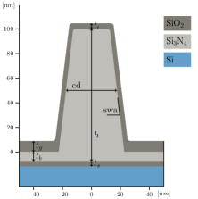
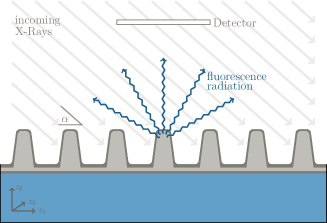
Figure 1: Left: Cross-section of one grating line with characterizing parameters. Right: Cross-section of the grating with incoming X-rays (typically in $z_{3}$ direction) and emitted fluorescence radiation.

To determine the parameters, we want to apply the GIXRF technique recently established to find the geometry parameters of nanostructures and its atomic composition [2, 8].

Experimental Setting.

In GIXRF, the angles $\alpha_{i}$, $i=1,\ldots,n$ between an incident monochromatic X-ray beam and the sample surface is varied around a critical angle for total external reflection. Depending on the local field intensity of the X-ray radiation, atoms are ionized and are emitting a fluorescence radiation. The resulting detected fluorescence radiation $(F(\alpha_{i};x))_{i=1}^{n}$ is characteristic for the atom type.

Besides direct experimental measurements of the fluorescence $F$, its mathematical modeling at each angle $\alpha$ can be done in two steps, namely by computing the intensity of the local electromagnetic field $E$ arising from the incident wave (X-ray) with angle $\alpha$ and then to use its modulus to obtain the fluorescence value $F(\alpha,x)$. The propagation of $E$ is in general described by Maxwell’s equations and simplifies for our specific geometry to the partial differential equation

$$\operatorname{\nabla_{z}}\cdot\left(\mu(z;x)^{-1}\operatorname{\nabla_{z}}E(z)\right)-\omega^{2}\varepsilon(z;x)\,E(z)=0,\quad z\in\mathbb{R}^{2}.$$ (9)

Here $\omega$ is the frequency of the incident plane wave, $\varepsilon$ and $\mu$ are the permittivity and permeability depending on the grating parameters $x$, resp. From the 2D distribution of $E$ in (9), more precisely from the resulting field intensities $|E|$, the fluorescence radiation $F(\alpha;x)$ at the detector can be calculated by an extension of the Sherman equation [17]. This computation requires just the appropriately scaled summation of the values of $|E|^{2}$ on the FEM mesh of the Maxwell solver used. The really time consuming part is the numerical computation of $E$ for each angle $\alpha_{i}$, $i=1,\ldots,n$ by solving the PDE (9).

Numerical treatment.

In order to compute $E$ given by (9) with appropriate boundary conditions, we employ the finite element method (FEM) implemented in the JCMsuite software package to discretize and solve the corresponding scattering problem on a bounded computational unit cell in the weak formulation as described in [13]. This formulation yields a splitting of the complete $\mathbb{R}^{2}$ into an interior domain hosting the total field and an exterior domain, where only the purely outward radiating scattered field is present. At the boundaries, Bloch-periodic boundary conditions are applied in the periodic lateral direction and an adaptive perfectly matched layer (PML) method was used to realize transparent boundary conditions.

Surrogate NN model

The evaluation of the fluorescence intensity $F$ for a single realization of the parameters $x$ involves solving (9) for each angle $\alpha_{i}$, $i=1,\dots,n$. Since this is very time consuming, we learn instead a simple feed-forward neural network with one hidden layer with $256$ nodes and ReLU activation as surrogate $f\colon\mathbb{R}^{d}\to\mathbb{R}^{n}$ of $F$ such that the $L^{2}$ error between $\left(f_{i}(x)\right)_{i=1}^{n}$ and $\left(F(\alpha_{i};x)\right)_{i=1}^{n}$ becomes minimal. The network was trained on roughly $10^{4}$ sample pairs $(F,x)$ which were numerically generated as described above in a time consuming procedure. The $L^{2}$-error of the surrogate, evaluated on a separate test set containing about $10^{3}$ sample pairs was smaller than $2\cdot 10^{-3}$. This is sufficient for the application, since we have measurement noise on the data of at least one order of magnitude larger for both the experimental data and the synthetic study. Hence we neglect the approximation error of the FE model and the surrogate further on.

4 Numerical Results

In this section, we solve the statistical inverse problem of GIXRF using the Bayesian approach with an INN and the MCMC method based on our surrogate NN forward model for virtual and experimental data. Note that obtaining training data for the forwardNN took multiple days of computation on a compute server with 120 CPUs. We compare the resulting posterior distributions and the computational performance. To the best of our knowledge, this was not done in the literature so far for any forward model.

The fluorescence intensities for the silicon nitride layer of the lamellar grating depicted in Fig. 1 were measured for $n=178$ different incidence angles $\alpha_{i}$ ranging from $0.8^{\circ}$ to $14.75^{\circ}$. The seven parameters of the grating were considered to be uniformly distributed according to the domains listed in Tab. 1.

Parameter:	$h$	$cd$	$\mathrm{swa}$	$t_{t}$	$t_{b}$	$t_{g}$	$t_{s}$
Domain:	$[85,\,100]$	$[45,\,55]$	$[76,\,88]$	$[2,\,4]$	$[0,\,5]$	$[2,\,10]$	$[0.1,\,3]$

Table 1: Domains of the different parameters. Units are given in $[\mathrm{nm}]$ for all parameters except the sidewall angle ($\mathrm{swa}$), which is given in $[^{\circ}]$.

To gain maximal performance of the MCMC method, we utilize an affine invariant ensemble sampler for the Markov-Chain Monte Carlo algorithm [5]. This allows parallel computations with multiple Markov chains and reduces the number of method specific free parameters for the MCMC steps. The error parameter $b$ is usually a priori unknown and is thus subject to expert knowledge. However, MCMC algorithms can introduce those as additional posterior hyperparameters for reconstruction by a slight modification of the prior. Define $\tilde{x}\coloneqq(x,b)\sim P_{\tilde{x}}$, where $P_{\tilde{x}}$ is given by the density $p_{(x,b)}=p_{x}\,p_{b}$ for uniform $p_{b}$. Using this error model in the likelihood in (1), we obtain $p_{y|(x,b)}$. Then the MCMC algorithm applied to $p_{(x,b)|y}$ yields the distribution of the parameter $b$ as well.

To approximate the INN that pushes the example density forward to the posterior one, we learn an INN with $L=10$ layers. Each subnetwork of each layer is chosen as a two layer ReLU feedforward network with $256$ hidden nodes in each layer. The network is trained on the empirical counterpart of the loss (8) by sampling from a standard Gaussian distribution using an adaptive moment estimation optimization (Adam) algorithm, see [9]. We trained for 80 epochs, an epoch consists of 40 parameter updates with a batch-size of 200. The learning rate is lowered by a factor of 0.1 every 20 epochs. The INN model is built and trained with the freely available FrEIA software package .

The time that is required to obtain $2\cdot 10^{4}$ posterior samples via the MCMC algorithm varies between $1.5$ and $3.5$ hours on a standard Laptop. In comparison the training of the INN takes less than $20$ minutes, and $2\cdot 10^{4}$ independent posterior samples are generated in less than one second.

4.1 Synthetic Data

As a first application, we perform a virtual experiment for the GIXRF to obtain a problem with known ground truth. To approach that, we pick a pair $(x_{\mathrm{true}},f(x_{\mathrm{true}}))$ and vary $b\in\{10^{-2},3\cdot 10^{-2},10^{-1}\}$. Using these values of $b$ we obtain a synthetic noisy measurement according to $y_{\mathrm{meas}}=y_{\mathrm{true}}+\varepsilon$ for various realizations of $\varepsilon$ of $\mathcal{N}(0,b^{2}\operatorname{diag}(y_{\mathrm{true}}^{2}))$. For the computation of the INN, we set $b$ according to the true value, whereas MCMC is able to estimate a distribution of the parameter $b$ for given $y_{\mathrm{meas}}$. For the application of both MCMC and INN, we set $y=y_{\mathrm{meas}}$ and $w=y_{\mathrm{meas}}$ (note that we regard $w=y_{\mathrm{meas}}$ as a constant). Fig. 2 displays the one dimensional marginals of the posterior for both the MCMC and the INN approach alongside the ground truth for three different values of $b$.

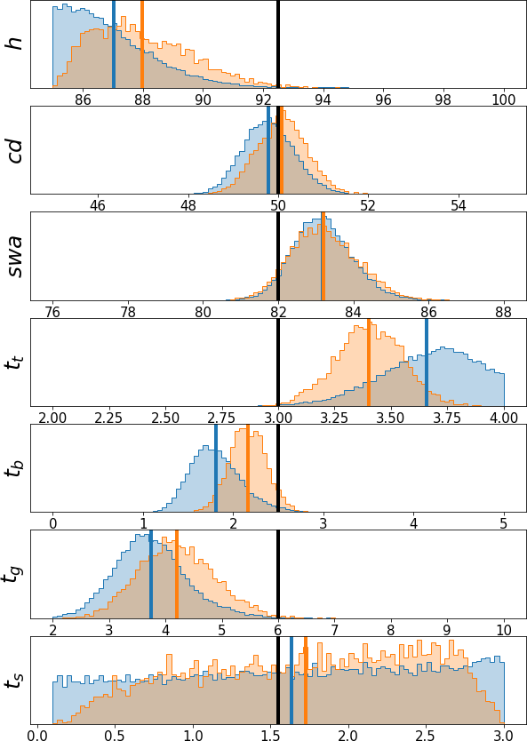
(a) $b=0.1$

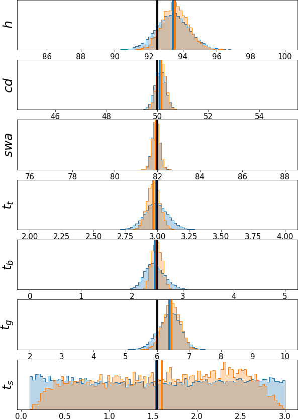
(b) $b=0.03$

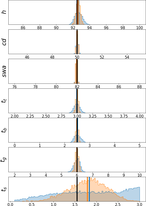
(c) $b=0.01$

Figure 2: One dimensional marginals of posterior samples for different values of $b$ generated by MCMC (blue) and INN (orange) together with their means as solid lines. The values of the ground truth $x_{i}$, $i=1,\ldots,7$ are displayed as solid black lines.

First one sees that the width of the marginals decreases as $b$ gets smaller. Comparing the INN and MCMC marginals shows an almost identical shape and support for most of the parameters, where the uncertainties obtained by the INN tend to be a bit smaller. The posterior means of the MCMC and INN approach are in proximity of each other relative to the domain size, in particular in the cases, where $b$ is smaller. It is remarkable that although the reconstruction in $b=0.1$ is far-off from the ground truth, both methods agree in their estimate. This can be explained by the large magnitude of noise. The noise realization for $b=0.1$ changes the measurements drastically such that a different parameter configuration becomes more likely. Furthermore, both methods identify the last parameter to be the least sensitive.

4.2 Experimental Data

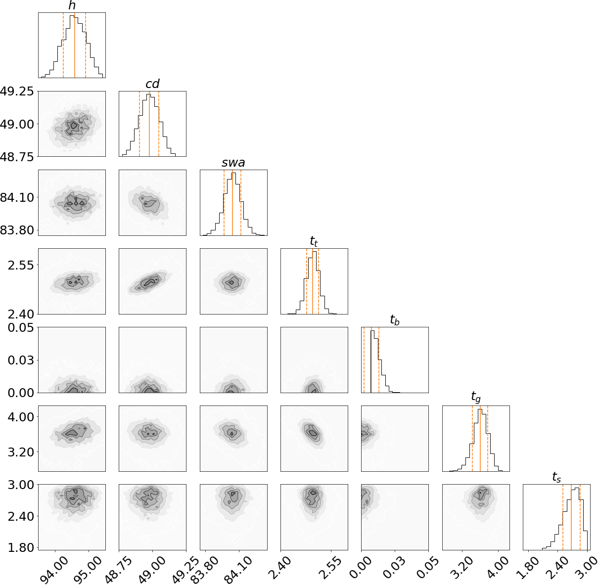
(a) INN.

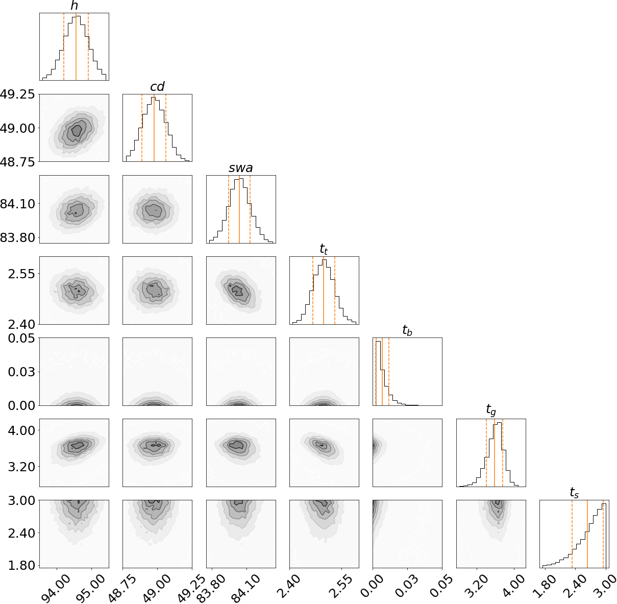
(b) MCMC.

Figure 3: Comparison of 2D densities of the posterior for $y_{\mathrm{meas}}$ calculated via the different methods. The straight vertical line depicts the mean, the dashed ones the standard deviation.

In the next experiment, we use fluorescence measurements $y_{\mathrm{meas}}=\left(F(\alpha_{i};x)\right)_{i=1}^{n}$ obtained from an GIXRF experiment. Here neither exact values of the parameters $x$ nor of the noise level $b$ are available. In the noise model (1) we use $w=y_{\mathrm{meas}}$. To train the INN we set the value $b$ to the mean $0.02$ of the reconstructed $b$ obtained by the MCMC algorithm. Fig. 3 depicts the one and two dimensional marginals of the posterior for both the MCMC and the INN calculations on a smaller subset of the parameter domain. The means and supports of the posteriors agree well. Fig. 3 also shows that the posterior is mostly a sharp Gaussian. The $Si_{3}N_{4}$ height etch offset $t_{b}$ is known to be close to zero for the real grating, which explains the non-Gaussian accumulation at the boundary of the interval. Similar holds true for the height of the lower $SiO_{2}$ layer.

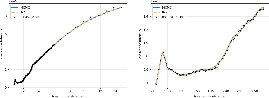
Figure 4: Forward fit of posterior means obtained by INN (orange) and MCMC (blue). Measurement data are represented by black points. The right image is a zoom into the left one.

Finally, we apply the forward model $f$ to the componentwise mean of the sampled posterior values $x\in\mathbb{R}^{7}$. The results are shown in Fig. 4. The resulting $f(x)$ fits both for the MCMC and for the INN quite well with the experimental measurement $y_{\mathrm{meas}}$. The differences in the mean and shape of the posteriors seem to be small and may be caused by small numerical or model errors.

5 Conclusions

We have shown that INNs provide comparable results to established MCMC methods in sampling posterior distributions of parameters in GIXRF, but outperform them in terms of computational time. Moreover INNs are more flexible for different applications and are expected to perform well in high dimensions. Since INNs are often used in very high-dimensional problems, such as generative modeling of images, this suggests that our approach could scale well to more challenging high-dimensional problems. So far, we considered only a single measurement $y_{\mathrm{meas}}$, but extensions to capture different measurements seem to be feasible. Furthermore, we will figure out, whether the noise parameter $b$ can be learned as well in the INN framework. Finally, we intend to have a closer look at multimodal distributions as done, e.g., in [6].

References

- [1] C. Andrieu, N. de Freitas, A. Doucet, and M. I. Jordan. An introduction to MCMC for machine learning. Machine Learning, 50:5–43, 2003.
- [2] A. Andrle, P. Hönicke, P. Schneider, Y. Kayser, M. Hammerschmidt, S. Burger, F. Scholze, B. Beckhoff, and V. Soltwisch. Grazing incidence x-ray fluorescence based characterization of nanostructures for element sensitive profile reconstruction. In Modeling Aspects in Optical Metrology VII, volume 11057, page 110570M. International Society for Optics and Photonics, 2019.
- [3] L. Ardizzone, J. Kruse, C. Rother, and U. Köthe. Analyzing inverse problems with invertible neural networks. In 7th International Conference on Learning Representations, ICLR 2019, New Orleans, LA, USA, May 6-9, 2019, 2019.
- [4] L. Dinh, J. Sohl-Dickstein, and S. Bengio. Density estimation using real NVP. In 5th International Conference on Learning Representations, ICLR 2017, Toulon, France, April 24-26, 2017, Conference Track Proceedings, 2017.
- [5] D. Foreman-Mackey, D. W. Hogg, D. Lang, and J. Goodman. EMCEE: The MCMC hammer. Publications of the Astronomical Society of the Pacific, 125(925):306–312, 2013.
- [6] P. Hagemann and S. Neumayer. Stabilizing invertible neural networks using mixture models. ArXiv preprint arXiv:2009.02994, 2020.
- [7] M.-A. Henn, H. Gross, S. Heidenreich, F. Scholze, C. Elster, and M. Bär. Improved reconstruction of critical dimensions in extreme ultraviolet scatterometry by modeling systematic errors. Measurement Science and Technology, 25(4):044003, 2014.
- [8] P. Hönicke, A. Andrle, Y. Kayser, K. V. Nikolaev, J. Probst, F. Scholze, V. Soltwisch, T. Weimann, and B. Beckhoff. Grazing incidence-x-ray fluorescence for a dimensional and compositional characterization of well-ordered 2d and 3d nanostructures. Nanotechnology, 31(50):505709, 2020.
- [9] D. P. Kingma and J. Ba. Adam: A method for stochastic optimization. In Y. Bengio and Y. LeCun, editors, 3rd International Conference on Learning Representations, ICLR 2015, San Diego, CA, USA, May 7-9, 2015, Conference Track Proceedings, 2015.
- [10] J. Kruse, G. Detommaso, R. Scheichl, and U. Köthe. HINT: Hierarchical invertible neural transport for density estimation and Bayesian inference. ArXiv preprint arXiv:1905.10687, 2020.
- [11] C. Mack. Fundamental principles of optical lithography: the science of microfabrication. John Wiley & Sons, 2008.
- [12] Y. Marzouk, T. Moselhy, M. Parno, and A. Spantini. Sampling via measure transport: An introduction. Handbook of Uncertainty Quantification, page 1–41, 2016.
- [13] J. Pomplun, S. Burger, L. Zschiedrich, and F. Schmidt. Adaptive Finite Element Method for Simulation of Optical Nano Structures. Physica Status Solidi (B), 244(10):3419–3434, 2007.
- [14] G. Rizzuti, A. Siahkoohi, P. A. Witte, and F. J. Herrmann. Parameterizing uncertainty by deep invertible networks, an application to reservoir characterization. ArXiv preprint arXiv:2004.07871, 2020.
- [15] W. Rudin. Real Analysis. McGraw-Hill, 3rd edition, 1987.
- [16] A. Siahkoohi, G. Rizzuti, M. Louboutin, P. A. Witte, and F. J. Herrmann. Preconditioned training of normalizing flows for variational inference in inverse problems. ArXiv preprint arXiv:2101.03709, 2021.
- [17] V. Soltwisch, P. Hönicke, Y. Kayser, J. Eilbracht, J. Probst, F. Scholze, and B. Beckhoff. Element sensitive reconstruction of nanostructured surfaces with finite elements and grazing incidence soft x-ray fluorescence. Nanoscale, 10(13):6177–6185, 2018.