A simpler spectral approach for clustering in directed networks

Abstract

We study the task of clustering in directed networks. We show that using the eigenvalue/eigenvector decomposition of the adjacency matrix is simpler than all common methods which are based on a combination of data regularization and SVD truncation, and works well down to the very sparse regime where the edge density has constant order. Our analysis is based on a Master Theorem describing sharp asymptotics for isolated eigenvalues/eigenvectors of sparse, non-symmetric matrices with independent entries. We also describe the limiting distribution of the entries of these eigenvectors; in the task of digraph clustering with spectral embeddings, we provide numerical evidence for the superiority of Gaussian Mixture clustering over the widely used k-means algorithm.

1 Introduction

The proverbial effectiveness of spectral clustering (“good, bad, and spectral”, said Kannan et al. (2004)), observed for long by practitioners, begins to be well-understood from a theoretical point of view. More and more problem-specific spectral algoritms are periodically designed, with better computational performance and accuracy. Most of the theoretical studies used to be concentrated on symmetric interactions and undirected networks, but over the last decade a flurry of works has tackled the directed case: the 2013 survey Malliaros and Vazirgiannis (2013) gave an account of the richness of directed network clustering, but since then the field expanded in various directions.

In directed networks, the directionality of interactions is taken into account. This is more realistic from a modeling point of view, but at the cost of intricate technicalities in the analysis. In this context, the aim of this paper is to take a step back at spectral algorithms and convince the readers of a simple, yet largely unnoticed truth: when clustering directed networks, directly using eigenvalues and eigenvectors (as opposed to SVD) of the untouched adjacency matrix (as opposed to symmetrized and/or regularized versions), works very well, especially in harder and sparser regimes. This statement was hinted in some works, but remained essentially ignored and not backed by theoretical results. In this paper, our goal is to rigorously prove and illustrate this statement.

Spectral clustering of directed networks: overview and related work

As well-summarized in Von Luxburg (2007), spectral algorithms often consist of three steps: (1) a matrix representation of the data, (2) a spectral truncation procedure, and (3) a geometric clustering method on the eigen/singular vectors.

The matrix representation depends on the nature of the data and interaction measurements. Early works were focused on symmetric interactions: the interaction $A_{x,y}$ between two nodes $u,v$ was considered undirected, ie $A_{x,y}=A_{x,y}$. The matrix of interactions $A$ is then hermitian. But in many applications, the interaction are intrinsically directional, with $A_{x,y}$ and $A_{y,x}$ not necessarily equal, or, equivalently, the network is directed. This covers a wider range of models: buyer/seller networks, ecologic systems with predator-prey interactions, citations in scientific papers, etc.

Forerunners in digraph clustering avoided using the interaction matrix $A$; one reason for that is the lack of an orthogonal decomposition for non-normal matrices. Instead, they represented their data with naive symmetrizations of $A$, such as $A+A^{*}$ or the so-called co-citation and bibliometric symmetrizations $AA^{*}$ and $A^{*}A$ (which reduces to studying the SVD of $A$), see Satuluri and Parthasarathy (2011) for an overview. Variants of the graph Laplacian were then introduced (Chung (2005)); they were hermitian but incorporated in some way the directionality of edges and were provable relaxations of normalized-cut problems (see Leicht and Newman (2008) and references in (Malliaros and Vazirgiannis, 2013, §4.2-4.3)); others used random-walks approaches similar to PageRank (Chen et al. , Pentney and Meila (2005)). It is quite striking that in the survey Malliaros and Vazirgiannis (2013), the authors classify the clustering methods (Chap. 4 therein) without mentioning the use of the adjacency matrix of directed networks. Implicit in these early works was the belief that directed networks need to be transformed or symmetrized. More recently, Cucuringu et al. (2019) and Laenen and Sun (2020) cleverly introduced $\mathbb{C}$-valued Hermitian matrices.

The use of adjacency matrices was advocated later, notably in Li et al. (2015), and several more theoretical works, among them Mariadassou et al. (2010); Zhou and Amini (2019); Van Lierde et al. (2019). These works can roughly be split in two categories. On one side, the authors of many papers seemed reluctant to use eigenvalues of non-symmetric matrices, and favored the SVD instead, whose theoretical analysis is tractable in some cases. This is notably the case for Sussman et al. (2012); Mariadassou et al. (2010); Zhou and Amini (2019). However, as we’ll see later, the SVD for non-hermitian matrices suffers the same problem as the eigendecomposition of hermitian matrices: it is sensitive to heterogeneity, and thus less powerful in sparse regimes. On the other side, Li et al. (2015); Van Lierde et al. (2019); Chen et al. (2018) are closer in spirit to our work. They explicitly advocate the use of eigenvalues of non-symmetric matrices as a better option for inference problems. The theoretical analysis performed in Li et al. (2015); Van Lierde et al. (2019) allows them to guarantee performance in very specific cases, where the underlying graphs have a strong and dense structure (upper-triangular , cyclic or purely acyclic). In a different context (matrix completion), the paper Chen et al. (2018) was one of the first to prove the efficiency of eigenvalues of non-hermitian matrices in high-dimensional problems.

Spectral decompositions of network matrices are generally known to reflect some of the underlying interaction structure between the nodes; this non-rigorous statement has now been mathematically understood in a variety of ways, many of them based on a mathematical model for community networks called the stochastic block-model (Holland et al. (1983); Abbe (2017)). Any clustering algorithm can be tested on synthetic data from the SBM to evaluate the reconstruction accuracy, that is, the number of nodes which have been correctly assigned to their community by the algorithm. In this work, we deal with a vast generalization of SBMs, the weighted, inhomogeneous, directed Erdős-Rényi random graph.

Definition 1.

Let $P,W$ be two real $n\times n$ matrices, with $P$ having entries in $[0,1]$. A random weighted graph is defined as follows: the edge set is $V=[n]$; each one of the $n^{2}$ potential edges $(x,y)\subset V\times V$ is present in the graph with probability $P_{x,y}$ and independently of the others; if present, its weight is $W_{x,y}$. The resulting directed graph will be noted $G=(V,E)$ and its weighted adjacency matrix $A$ is defined by $A_{x,y}\coloneqq W_{x,y}\mathbf{1}_{(x,y)\in E}$.

This allows for virtually any structure: classical block-models (assortative or disassortative), cyclic structures (Van Lierde et al. (2019)), path-wise structures (Laenen and Sun (2020)), overlapping communities (Ding et al. (2016)), bipartite clustering when both sides have the same size (Zhou and Amini (2019, 2018)), contextual information on the edges…

In SBMs, a key parameter is the density $d$, the number of edges divided by the size $n$. For inference problems, a lower density means a sparser information. Analyzing the performance of spectral clustering methods can be done using classical perturbation results in regimes where $d$ is large, often of order $n$ (the ‘dense’ regime), see Rohe et al. (2011) for instance. However, many real-world networks lie in sparser regimes $d\ll n$, like $d\lesssim\log(n),d\to\infty$ (the ‘semi-sparse regime’) or even $d=O(1)$ (the ‘sparse regime’), a radically difficult regime in which node degrees are extremely heterogeneous and the graph is not even connected. This behaviour has an impact on spectral quantities when they satisfy Fisher-Courant-Weyl inequalities, like eigenvalues of normal matrices or SVD of non-normal ones, deeply reducing their performance, see Benaych-Georges et al. (2019). This is why most theoretical works (for both directed and undirected models) were concentrated on $d\sim\log(n)$ regimes (Abbe et al. (2020b) among others). In the sparse undirected regime, the celebrated Kesten-Stigum threshold (Bordenave et al. (2018)) gives a spectral condition for the emergence of a second eigenvalue $\lambda_{2}$, beyond the Perron one, in the spectrum of the non-backtracking matrix. The entries of its eigenvector are correlated with the block structure when there are two blocks. In this paper, we describe a general theory of directed Kesten-Stigum-like thresholds for every directed sparse SBM, irregardless of the number of blocks, their size, etc.

Contributions.

We prove a Master Theorem describing the sharp asymptotics of eigenvalues and eigenvectors of sparse non-symmetric matrices with independent entries, like adjacency matrices of inhomogeneous directed Erdős-Rényi graphs. This is of independent interest in the field of random matrices. We show how to apply this theorem to the directed SBM and we introduce an elementary community-detection algorithm based on the adjacency matrix. We show why using both left and right eigenvectors is mandatory in sparse regimes. We give numerical and heuristic evidence for why Gaussian Mixture clustering is much more adapted than the popular k-means algorithm. Finally, we illustrate the strength of our method on synthetic data.

Notations.

We use the standard Landau notations $o(\cdot),O(\cdot),\sim$; for $k$ integer, $[k]$ stands for $\{1,\dotsc,k\}$. The letters $u,v,w$ will be kept for vectors, the letters $x,y,z$ will be kept for elements of $[n]$ (nodes). We see vectors in $\mathbb{C}^{n}$ as functions from $[n]$ to $\mathbb{C}$, that is $u=(u(1),\dotsc,u(n))$. The notation $|u|_{p}$ stands for the $p$-norm of a vector, $|u|_{p}^{p}=|u(1)|^{p}+\dotsc+|u(n)|^{p}$. We drop the index $p$ iff $p=2$ (euclidean norm). If $M$ is a matrix, $\|M\|=\sup_{|u|=1}|Mx|$ and $\|M\|_{\infty}=\max M$. The Hadamard product of two matrices $A,B$ with the same shape is defined as the entrywise product: $(A\odot B)_{x,y}=A_{x,y}B_{x,y}$. The Frobenius norm is $\|M\|_{F}=\sqrt{\sum_{x,y}|M_{x,y}|^{2}}$.

2 The Master Theorem

Let $P,W$ be two real $n\times n$ matrices, with $P$ having entries in $[0,1]$. The weighted, inhomogeneous directed Erdős-Rényi model was defined in Definition 1. The weighted adjacency matrix will be noted $A$. We focus on the $n\to\infty$ limit and we suppose in the assumptions thereafter that the graph is sparse, the weights are bounded and the spectral decomposition of $\mathbf{E}[A]$ is not degenerate. Let $Q=\mathbf{E}[A]$ and $K=\mathbf{E}[A\odot A]$ be the first and second entrywise-moments of $A$, given by

$$Q=P\odot W\qquad\text{ and }\qquad K=P\odot W\odot W,$$ (1)

in other words $Q_{x,y}=P_{x,y}W_{x,y}$ and $K_{x,y}=P_{x,y}|W_{x,y}|^{2}$. Our assumptions are as follows:

1. $\|P\|_{\infty}=O(1/n)$ and $\|W\|_{\infty}=O(1)$.

2. The matrix $Q$ has rank $r=O(1)$, is real diagonalizable, and its $r$ eigenvalues $\mu_{i}$ are well-separated in the sense that there is a constant $c>0$ such that $|\mu_{i}-\mu_{j}|>c,|\mu_{j}|>c$.

3. the right (resp. left) unit eigenvectors $\varphi_{i}$ and $\xi_{i}$ associated with $\mu_{i}$ are delocalized, in that

   $$|\varphi_{i}|_{\infty},|\xi_{i}|_{\infty}=O\left(\frac{1}{\sqrt{n}}\right)$$ (2)

These assumptions will be commented later. We note $\rho=\|K\|$. The detection threshold is

$$\upvartheta=\max\left(\sqrt{\rho},\|W\|_{\infty}\right)$$

and we note $r_{0}$ the number of eigenvalues of $Q$ with modulus strictly greater than $\upvartheta$.

Definition 2.

Let $\mu_{i}$ be an eigenvalue of $Q$ with left and right unit eigenvectors $\varphi_{i},\xi_{i}$. If $|\mu_{i}|>\upvartheta$, the (left and right) eigendefects of $\mu_{i}$ are defined by

$$R_{i}=|(K-\mu_{i}^{2}I)^{-1}\varphi_{i}^{2}|_{1}\qquad\qquad L_{i}=|(K^{*}-\mu_{i}^{2}I)^{-1}\xi_{i}^{2}|_{1}$$ (3)

where $\varphi_{i}^{2},\xi_{i}^{2}$ are the entrywise squares of $\varphi_{i},\xi_{i}$.

These novel quantities will play a role of paramount importance in all this paper and will be commented later. Let us first state our main result, after which we will give some intuition on (3).

Theorem 3 (Master Theorem).

Under the above hypotheses, the following holds with probability going to $1$ when $n\to\infty$. The $r_{0}$ eigenvalues of $A$ with highest modulus, $\lambda_{1},\dotsc,\lambda_{r_{0}}$, are asymptotically equal to the $r_{0}$ eigenvalues of $Q$ with highest modulus: $|\lambda_{i}-\mu_{i}|=o(1)$. All the other $n-r_{0}$ eigenvalues of $A$ are asymptotically smaller than $\upvartheta$. Moreover, if $u_{i},v_{i}$ is a left/right pair of unit eigenvectors of $A$ associated with $\lambda_{i}$, and if $\varphi_{i},\xi_{i}$ is a left/right pair of unit eigenvectors of $Q$ associated with $\mu_{i}$, then

$$\left||\langle u_{i},\varphi_{j}\rangle|-\frac{|\langle\varphi_{i},\varphi_{j}\rangle|}{|\mu_{i}|\sqrt{R_{i}}}\right|=o(1)\qquad\text{ and }\qquad\left||\langle v_{i},\xi_{j}\rangle|-\frac{|\langle\xi_{i},\xi_{j}\rangle|}{|\mu_{i}|\sqrt{L_{i}}}\right|=o(1).$$ (4)

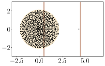
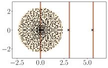
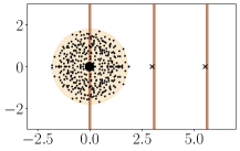
(a)	(b)	(c)

Figure 1: Spectra of inhomogeneous Erdős-Rényi graphs, with no weights, $n=1000$ nodes. The underlying connectivity matrix $P$ is a block-matrix; the inset of each picture shows a colorplot of $P$, with darker colors indicating higher values. The points are the eigenvalues of $A$. The brown lines indicate the non-zero eigenvalues $\mu_{i}$ of $Q$. The beige circle behind the eigenvalues has radius $\upvartheta$. The outliers close to $\mu_{i}$ for $i\in[r_{0}]$ are visible for each picture.

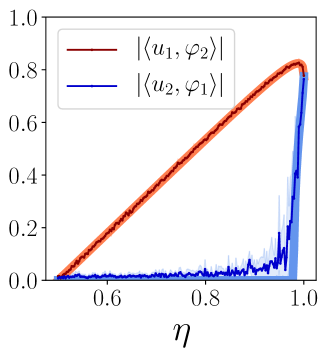
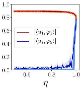
Figure 2: Bottom: An illustration of the ‘right eigenvector part’ of the Master Theorem, for the two-block SBM described in Theorem 8 with parameters $s=10$ and $\eta$ ranging from $0.5$ to $1$. For each $\eta$ the results are averaged over $50$ samples (coloured zone is for standard errors). The thin darker lines are $\langle u_{i},\varphi_{j}\rangle$ for $i,j\in\{1,2\}$. The thick lighter lines are our theoretical predictions $\langle\varphi_{i},\varphi_{j}\rangle/\mu_{i}\sqrt{R_{i}}$. The second eigenvector begins to be informative as soon as the second eigenvalue reaches $\upvartheta$, which happens at around $0.979$ in agreement with our predictions.

The eigendefects in Definition 2 measure how much the eigenequations of $Q$ can be ‘entrywise squared’. For instance, let $\mu$ be an eigenvalue of $Q$ with eigenvector $\varphi$. Then, $(Q-\mu_{i}I)\varphi_{i}=0$. But is $\varphi^{2}_{i}$ an eigenvector of $K$ with eigenvalue $\mu_{i}^{2}$ ? If $i\in[r_{0}]$, the answer is obviously no since $\mu_{i}^{2}>\|K\|$; then, the quantity $1/|(K-\mu_{i}^{2})^{-1}\varphi_{i}^{2}|_{1}$ appearing in the theorem above is a measure of how far $\varphi_{i}^{2}$ is from being a $\mu_{i}^{2}$-eigenvector of $K$. The theorem says that when $\mu_{i}$ is gives rise to an outlier $\lambda_{i}$ in the spectrum of $A$, then the overlap $\langle u_{i},\varphi_{i}\rangle$ between the real eigenvector and the sample eigenvector is higher when $\varphi_{i}^{2}$ is far from being an eigenvector of $K$. At a high level, this surprising and new phenomenon comes from an elementary formula regarding the covariance of Poisson sums (see Lemma 21 in Appendix B), and we conjecture that a similar phenomenon will hold for every random matrix model which is asymptotically Poisson.

Remark 4 (Comments on the hypotheses. ).

Under Hypothesis 1, if $\|P\|_{\infty}\leqslant C/n$, then the expected degree of $x\in[n]$ is $d_{x}=P_{x,1}+\dotsb+P_{x,n}\leqslant C$ so the average density $d$ is smaller than $C$ (sparse regime). Our proof holds in the semi-sparse regime $d\to\infty,d=n^{o(1)}$, but it is not our primary motivation. In this semi-sparse regime is can be proved that $|\mu_{i}|\sqrt{R_{i}}$ goes to $1$, resulting in perfect alignment $\langle u_{i},\varphi_{i}\rangle\to 1$.

Real diagonalizability in Hypothesis 2 is here to simplify the proof but the Master Theorem will hold for complex eigendecompositions. The low-rank assumption is standard in the litterature; it can be relaxed by replacing the rank with the effective rank, as in Bordenave et al. (2020). The separation assumption is not necessary for eigenvalue asymptotics, but strong separation is necessary for eigenvector overlaps.

Note that every bound in the hypotheses (such as the bound on $W$, the rank or the delocalization) can be extended to $n^{o(1)}$ at virtually no cost.

Theorem 3 follows the line of research initiated in Massoulié (2014); Bordenave et al. (2018) and continued by different works, among which Stephan and Massoulié (2020); Bordenave et al. (2020); Pal and Zhu (2019). We give an overview of the proof of Theorem 3 in Appendix B.

3 Spectral embeddings of directed SBM

3.1 Model definition

A powerful aspect of our Master Theorem lies in its application to clustering in directed stochastic blockmodels. In the following, we fix a number of clusters $r$, and a number of vertices $n$, understood to be large. Let $\sigma_{g},\sigma_{d}:[n]\mapsto[r]$ be the left and right cluster assignments; that is, a vertex $x$ is said to be in the $i$-th left (resp. right) cluster if $\sigma_{g}(x)=i$ (resp. $\sigma_{d}(x)=i$). Let $F$ be an arbitrary $r\times r$ matrix with positive entries; the directed SBM is then a random graph $G=([n],E)$ with vertex set $[n]$ and such that for each directed edge $(i,j)$, we have

$$\mathbb{P}((i,j)\in E)=\frac{F_{\sigma_{g}(i),\sigma_{d}(j)}}{n}.$$

The aim is then to recover the left (or right) cluster memberships, given an observation of $G$. Note that, for ease of exposition, we did not include weights: $W$ is thus the all-one matrix, and in this setting we have $Q=P=\mathbf{E}[A]$. It is relatively simple to compute the spectral decomposition of $Q$ in this setting:

Proposition 5.

Let $A$ be the adjacency matrix of $G$. The non-zero eigenvalues of $P=\mathbf{E}[A]$ are exactly those of the modularity matrix $F\Pi$, where

$$\Pi_{ij}=\frac{\left|\sigma_{g}^{-1}(j)\cap\sigma_{d}^{-1}(i)\right|}{n}.$$

Additionnally, the associated left eigenvectors of $P$ are constant on the right clusters, while the right eigenvectors are constant on the left clusters.

Therefore, as per our main theore, the left/right eigenvectors of the adjacency matrix of $G$ are close to their expectation, which is constant on the right/left clusters. We thus expect a clustering algorithm on those eigenvectors to be able to recover at least a fraction of the community memberships. We refer to Appendix D for a more complete spectral analysis of the matrix $P$, as well as a formulation of Theorem 3 suited to the SBM setting.

Remark 6.

Whenever $\sigma_{g}=\sigma_{d}$, as is often the case, both left and right eigenvectors are constant on the clusters; this effectively doubles the signal to recover $\sigma_{d}$.

An important question to ask is the following: how many eigenvectors of $A$ do we need to be able to reconstruct the clusters ? It is often assumed that $r$ eigenvectors are needed to recover the memberships (see e.g. Von Luxburg (2007)). However, in our DSBM setting, we propose the following heuristic:

Partial cluster recovery is possible as soon as the first $r_{0}$ eigenvectors of $\mathbf{E}[A]$
are sufficient to recover the clusters.

Here, $r_{0}$ is the same as in Theorem 3, and denotes the number of eigenvalues of $\mathbf{E}[A]$ that get reflected in the spectrum of $A$. Since we showed that the eigenvectors of $\mathbf{E}[A]$ are constant on the clusters, this is equivalent to the function $k\mapsto(\psi_{1}(k),\dots,\psi_{r_{0}}(k))$ being injective, where the $\psi_{i}$ are the right (resp. left) eigenvectors of $F\Pi$ (resp. $\Pi F$). This can happen when $r_{0}\ll r$, and even in some cases when $r_{0}=1$, which is a huge improvement on the threshold for reconstruction. Additional eigenvectors may of course increase the recovery accuracy; however, in some cases, the additional information they bring is nullified by the increase in dimensions for the clustering algorithms.

3.2 SBM with a pathwise structure

General case.

We restrict to the classical SBM described earlier, with a specific shape known as pathwise structure, and notably studied in Laenen and Sun (2020). It is a good model for flow data. In this model, we have $\sigma_{d}=\sigma_{g}$, and the clusters partition $[n]$ in $r$ parts of equal size. The underlying $r\times r$ connectivity $F$ is given by

$$F=s\begin{pmatrix}1/2&\eta\\ 1-\eta&1/2&\eta\\ \\ &\ddots&\ddots&\ddots\\ \\ &&1-\eta&1/2&\eta\\ &&&1-\eta&1/2\end{pmatrix}$$ (5)

where $s>1$ is the density parameter and $\eta\in[1/2,1]$. The modularity matrix is therefore given by $F/r$. The matrix $F$ shown in (5) is a tridiagonal Toeplitz matrix; such matrices have been extensively studied and their eigendecomposition is known (see Appendix E.3): as a result, cluster recovery is possible as soon as the top eigenvalue of $F/r$ is at least one. This happens in particular whenever $s\geq 2r$.

Two blocks: explicit computations.

In the case of two blocks $r=2$ with the same size $n/2$, the connectivity matrix $F$ is equal to

$$F=\begin{pmatrix}s/2&s\eta\\ s(1-\eta)&s/2\end{pmatrix}$$ (6)

Define the parameter $\theta=2\sqrt{\eta(1-\eta)}$. The spectral structure of $F$ is described in the following lemma:

Lemma 7.

The two eigenvalues of $F$ are $\upsilon_{1}=s\frac{1+\theta}{2}$ and $\upsilon_{2}=s\frac{1-\theta}{2}$, with corresponding unit right eigenvectors $f_{i}$ and unit left eigenvectors $f_{i}$ given by

$$f_{1}=(\sqrt{\eta},\sqrt{1-\eta}), g_{1}=(\sqrt{1-\eta},\sqrt{\eta}),$$

$$f_{2}=(\sqrt{\eta},-\sqrt{1-\eta}), g_{2}=(\sqrt{1-\eta},-\sqrt{\eta}).$$

The eigenvectors of $P$ thus verify

$$\varphi_{i}(x)\propto f_{i}(\sigma(x))\qquad\text{and}\qquad\xi_{i}(x)\propto g_{i}(\sigma(x)),$$

and Theorem 3 applies in this setting:

Theorem 8.

Under the above assumptions, with high probability the following holds.

1) If $s<4(1+\theta)/(1-\theta)^{2}$, then $r_{0}=1$. The Perron eigenvalue of $A$, namely $\lambda_{1}$, is asymptotically equal to $\upsilon_{1}/2$, and all the other eigenvalues have modulus asymptotically smaller than $\sqrt{\upsilon_{1}/2}$. Moreover, if $u_{1},v_{1}$ is a left/right pair of unit eigenvectors associated with $\lambda_{1}$, then $\lim_{n\to\infty}|\langle u_{1},\varphi_{1}\rangle|=\lim_{n\to\infty}|\langle v_{1},\xi_{1}\rangle|=a_{1,1}$ where $a_{1,1}$ is a completely explicit function of $s,\eta$ that satisfies

$$a_{1,1}=1-\frac{2}{s}\cdot\frac{1+\theta^{2}}{(1+\theta)^{2}}+O\left(\frac{1}{s^{2}}\right)$$

2) If instead $s<4(1+\theta)/(1-\theta)^{2}$, then $r_{0}=2$. The Perron eigenvalue of $A$, namely $\lambda_{1}$, is asymptotically equal to $s\upsilon_{1}/2$, the second eigenvalue $\lambda_{2}$ is asymptotically equal to $\upsilon_{2}/2$ and all the other eigenvalues have modulus asymptotically smaller than $\sqrt{\upsilon_{1}/2}$.

Moreover, if $u_{i},v_{i}$ is a left/right pair of unit eigenvectors associated with $\lambda_{i}$ for $i=1,2$, then $\lim_{n\to\infty}|\langle u_{1},\varphi_{1}\rangle|=\lim_{n\to\infty}|\langle v_{1},\xi_{1}\rangle|=a_{1,1}$ as above, and additionnally $\lim_{n\to\infty}|\langle u_{2},\varphi_{2}\rangle|=\lim_{n\to\infty}|\langle v_{2},\xi_{2}\rangle|=a_{2,2}$ with $a_{2,2}$ a completely explicit function of $s,\eta$ that satifies

$$a_{2,2}=1-\frac{2}{s}\cdot\frac{1+\theta^{2}}{(1-\theta)^{2}}+O\left(\frac{1}{s^{2}}\right).$$

The threshold $s>4(1+\theta)/(1-\theta)^{2}$ can also be rewritten as $\eta>\eta(s)$, where $\eta$ is an explicit function of $s$ (see equation (48) in the Appendix). This will be the preferred formulation through the rest of the paper. Note that $\eta(s)$ decreases to $1/2$ quite slowly: as an example, we have $\eta(10)\approx 0.979$ and $\eta(50)\approx 0.885$, and it can be shown that $\eta(s)\sim cs^{-1/4}$.

4 Geometric clustering and community detection

Our Master Theorem describes the information given by the spectral embedding $\mathcal{X}$ on the underlying model. Most spectral clustering pipelines then perform geometric clustering based on $\mathcal{X}$.

4.1 Algorithm and measure of performance

Our algorithm computes the left and right eigenvectors $x_{i},y_{i}$ associated with the $r_{0}$ largest eigenvalues of $M$, then defines an embedding of the nodes of $[n]$ in $\mathbb{R}^{2k}$ by setting

$$\mathcal{X}^{A}(x)=(u_{1}(x),\dotsc,u_{r_{0}}(x),v_{1}(x),\dotsc,v_{r_{0}}(x)).$$ (7)

Then, we cluster these $n$ points using the Gaussian Mixture Model for clustering (McLachlan and Basford ). We insist on the fact that no data preprocessing is needed: no high-degree trimming, no pruning, no normalization. The complexity of our algorithm is similar to all the spectral clustering procedures: it needs the computation of at most $2r$ left/right eigenvectors where $r$ is generally $O(\log(n)^{c})$, and then doing a clustering method with at most $r$ clusters on a $n\times 2r_{0}$ embedding.

Remark 9.

The number $r_{0}$ is a priori problem-dependent. However, since $r_{0}\leqslant r$ and $r$ is low in most problems, one can loop over $r_{0}$ at a minor cost. The Master Theorem allows for a more reasonnable possibility, which is to directly estimate $r_{0}$ from the data as the number of isolated eigenvalues outside the bulk of the spectrum. This can easily be done either by visual inspection (see Figure 1) or by some ad hoc statistical rule and it does not require a priori knowledge of $r$ — unlike many methods in the litterature.

1:  Data: a $n\times n$ adjacency matrix $A$; a number of clusters $k$; a rank $r_{0}$.

2:  Compute the $r_{0}$ largest eigenvalues of $M$ and their unit left and right eigenvectors $u_{i},v_{i}$.  

3:  Define the spectral embedding $\mathcal{X}^{A}=\{\mathcal{X}_{x}^{A}:x\in[n]\}$ as in (7). 

4:  Apply a GMM-clustering method on the cloud $\mathcal{X}^{M}$.

5:  return  The partition of $[n]$ based on the output of GMM-clustering.

Algorithm 1 Spectral clustering of $n$ nodes, based on the adjacency matrix $A$.

In the stochastic block-model, we have a notion of ground-truth clustering $\sigma:V\to[k]$, where $\sigma(x)=i$ denotes the membership of node $x$ to the $i$-th cluster. If our procedure outputs a clustering $\hat{\sigma}$, the performance of this clustering is measured through the overlap, also called Rand Index: it is the proportion of pairs of nodes on which $\sigma$ and $\hat{\sigma}$ agree on membership, that is

$$\mathrm{ov}(\sigma,\hat{\sigma})=\frac{1}{\binom{n}{2}}\sum_{\{x,y\}}\mathbf{1}\{\sigma\text{ and }\hat{\sigma}\text{ agree on the edge }\{x,y\}\},$$ (8)

where ‘agree’ means that either $\sigma(x)=\sigma(y)$ and $\hat{\sigma}(x)=\hat{\sigma}(y)$, or $\sigma(x)\neq\sigma(y)$ and $\hat{\sigma}(x)\neq\hat{\sigma}(y)$. Without any information on $\sigma$, a blind guess for $\sigma(x)$ is to randomly assign $x$ to one of the $k$ clusters. This is called a dummy label, $\hat{\sigma}_{\mathrm{dummy}}$. The adjusted overlap is often preferred to the former:

$$\mathrm{aov}(\sigma,\hat{\sigma})=\frac{\mathrm{ov}(\sigma,\hat{\sigma})-\mathbf{E}[\mathrm{ov}(\sigma,\hat{\sigma}_{\mathrm{dummy}})]}{1-\mathbf{E}[\mathrm{ov}(\sigma,\hat{\sigma}_{\mathrm{dummy}})]}.$$ (9)

An adjusted overlap of $1$ indicates a perfect recovery of $\sigma$ (up to permutation), while an overlap of $0$ indicates that $\hat{\sigma}$ is not better than a dummy guess at recovering $\sigma$. In the litterature this is often called Adjusted Rand Index. It will be our measure of performance in our numerical experiments.

Remark 10 (notions of consistency).

Strong consistency of a procedure corresponds to $\mathrm{aov}=1$, that is: all the labels are correctly guessed. Weak consistency is when $\lim\mathrm{aov}=1$ when $n\to\infty$. Partial consistency is when $\liminf\mathrm{aov}>0$, meaning that the algorithm does strictly better than random guess, a task called detection. In the undirected setting, strong consistency is feasible in the regime $d/\log(n)\to\infty$ (Abbe et al. (2020b) and weak consistency as long as $d\to\infty$ (Gao et al. (2017) and the survey section therein). Note that in the sparse regime with $d$ constant (this paper), even weak consistency is not achievable because of a constant proportion of isolated nodes. Partial consistency in the undirected case was achieved in Bordenave et al. (2018); Mossel et al. (2015) under a spectral condition on the modularity matrix. We expect similar results to the ones above to hold in the undirected case.

4.2 Choice of the clustering algorithm

When it comes to the last step of spectral clustering, i.e. geometric clustering on the spectral embedding, the overwhelming choice of algorithm is the $k$-means (see for example Van Lierde et al. (2019); Zhou and Amini (2019)). It is very simple to implement, and its tractability allows for explicit performance bounds for spectral clustering (Cucuringu et al., 2019, Theorem 2). However, our numerical experiments (see Appendix A) show an interesting phenomenon: the addition of a second informative eigenvector appears to decrease the algorithm’s performance ! Our assumption is that the increase in dimensions for clustering caused by the introduction of the second eigenvector nullifies the additional information it brings. To the contrary, our experiments showed a significative increase in performance when using GMMs, although very little is known in terms of their theoretical footing. A mix of theoretical and empirical results allow us to present a simple explanation: the eigenvectors of $G$ are indeed close to a mixture of Gaussian distributions.

Theorem 11.

Consider the SBM as described in Section 3, with $\sigma_{d}=\sigma_{g}$. Assume that $\mu_{i}$ is an isolated informative eigenvalue of $P$, and let $u_{i}$ be a right eigenvector of the adjacency matrix of $G$ such that $|u_{i}|=\sqrt{n}$. Then we have the following convergence in distribution: for all $j\in[r]$,

$$\frac{1}{\operatorname{Card}(\sigma^{-1}(j))}\sum_{\sigma(x)=j}\delta_{u_{i}(x)}\xrightarrow[n\to+\infty]{d}Z_{i,j},$$

where $Z_{ij}$ is a random variable with known mean $\mu_{ij}$ and variance $\sigma_{ij}^{2}$ (see equation (52) in the Appendix). Similar results hold for the right eigenvector $v_{i}$.

In the above theorem, $\delta$ denotes the Dirac delta; the LHS is therefore simply the discrete measure on the entries of $u_{i}$ on the $j$-th community. The proof of this theorem, as well as an explicit derivation of $\mu_{ij}$ and $\sigma_{i}j$, can be found in the Appendix. It implies, in particular, that the distribution of $u_{i}$ can be seen as a mixture of $r$ different distributions.

We do not claim (and it is indeed false, see Remark 13) that $Z_{i,j}\sim\mathscr{N}(\mu_{ij},\sigma_{ij}^{2})$; however, numerical experiments performed in Figure 5 appear to show that, at least when the mean degree of the graph is large, the distribution of $u_{i}$ behaves as a mixture of Gaussian distributions. This brings us to the conjecture:

Conjecture 12.

When the top eigenvalue of $P$ goes to infinity, the distribution of $Z_{ij}$ approaches that of a normal random variable with same mean and variance.

If proven true, this conjecture would give theoretical footing to the performance of GMMs, whose edge over other algorithms is only observed empirically for now.

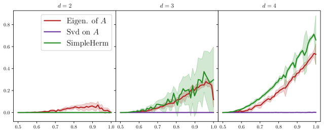
(a) $k=2$ blocks

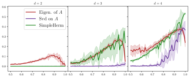
(b) $k=4$ blocks

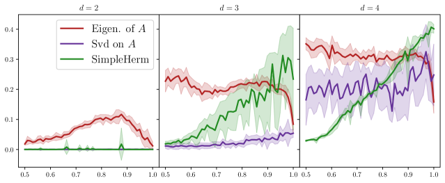
(c) $k=6$ blocks

Figure 3: Averages of labels reconstruction scores (adjusted overlaps), averaged over 20 runs for 50 values of $\eta$ ranging from $0.5$ to $1$, and for different mean degree $d$. The number of nodes is $n=2500$. Coloured zones are for standard errors of the corresponding method. The parameter $s$ corresponding to the various values $d$ are given in Table 1 page 1).

4.3 Numerical validation of our results

Tested methods.

We compare our Algorithm 1 with two other methods for digraph clustering. Both methods end with a k-means clustering on a spectral embedding. The first method uses the $k$ left and $k$ right top singular vectors of the adjacency matrix, where $k$ is the number of blocks. The second one is SimpleHerm: we define a complex Hermitian matrix by $H_{x,y}=\omega A_{x,y}+\overline{\omega}A_{v,u}$ where $\omega$ is the $\lceil 2\pi k\rceil$-th root of unity.We then use the eigenvector of the smallest eigenvalue $\lambda_{1}$ of $L=I-D^{-1/2}HD^{-1/2}$ with $D$ the diagonal degree matrix ($D_{x,x}=d^{+}_{x}+d^{-}_{x}$); since its entries are complex, it is viewed as an embedding on $\mathbb{R}^{2}$. This method was introduced in Laenen and Sun (2020), and was convincingly shown to outperform other classical methods in semi-sparse regimes.

SVD and our method are agnostic to problem structure, but SimpleHerm is well-fitted to flow networks. The performance guarantees of our method relies on the probabilistic properties of the SBM, while SimpleHerm satisfies deterministic Cheeger-like inequalities (see Laenen and Sun (2020)). It would be interesting to test these methods on more general models of directed networks.

Setting.

For $50$ values of $\eta$ equally spread between $0.5$ and $1$ we sampled $20$ directed SBMs with connectivity matrix $F$ as in (5) and with $n=2500$ nodes. The parameters are $k$, the number of blocks and equal to $2,4,6$ (the blocks have the same size $n/k$). For the parameter $s$, we chose the unique $s(d,k)$ so that the the mean degree of our model with $k$ blocks (given in the formula (42)) is equal to $d=2,3$ or $4$, see Table 1 at page 1 and discussion therein. We insist on the fact that the mean degree in our model is extremely low, and in particular stays under the $\log(n)=\log(2500)\approx 7.82$ barrier. Our performance measure is the adjusted overlap (9), between the labelling output by the tested method, and the true labelling.

Results.

The results of our experiments are in Figure 3. With extremely low degrees ($d=2$), our method (red curve) is the only one to catch a signal, the two other ones are unable to detect any community structure. For slightly higher $d=3,4$, our method seems to globally compare with SimpleHerm and be superior to SVD. When the asymmetry is closer to $1/2$ (hard regime), our method performs better, see for instance the very neat advantage for $k=6$ blocks, where our method reaches more than 20% overlap for $\eta\approx 1/2$, against no detection at all for the other methods. When $\eta$ approaches $1$, the performance of our method collapses back to low overlaps, while SimpleHerm has very high performances. We expect this phenomenon to be caused by the fact that when $\eta\to 1$, the eigenvectors of $F$ all align with $(1,0,\dotsc,0)$. On a side note, we remark that our method has a better precision, with the standard error (coloured zones) being generally smaller.

5 Conclusion and future prospects

We rigorously described the behaviour of a simple spectral embeddings, using the eigenvectors of non-symmetric matrices, and we numerically show that our algorithm using Gaussian Mixture clustering has suprisingly good results against state-of-the art methods in digraph clustering, especially in the difficult regime where the model density is $O(1)$. The main weakness of our theory is that it does not apply to rectangular matrices directly, but the randomsplit-squaring strategy as in Bordenave et al. (2020) is directly applicable here. Since our theory is new, we chose to keep the exposition as simple and general as possible, but many new directions seem to be promising: among them is the possibility to use the distance-matrix $A^{(\ell)}_{x,y}=\mathbf{1}_{d^{+}(x,y)\leqslant\ell}$ instead of $A$, which should result in a method which is more robust to adversarial perturbations, as in Abbe et al. (2020a); Stephan and Massoulié (2019). Regarding the gaussianity of the model, we conjecture that the fluctuations of the eigenvalues are Gaussian in the sparse regime; as mentioned, the fluctuations of the eigenvector entries will not be Gaussian, but we now explore a proof of the convergence of these fluctuations when the density of the model increases.

Appendix A Gaussian Mixture clustering and Gaussian fluctuations

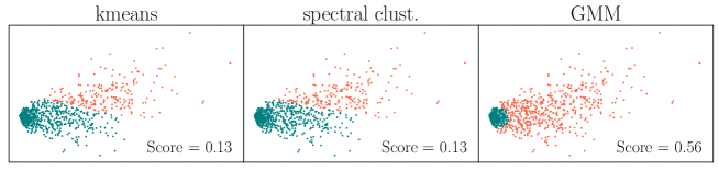
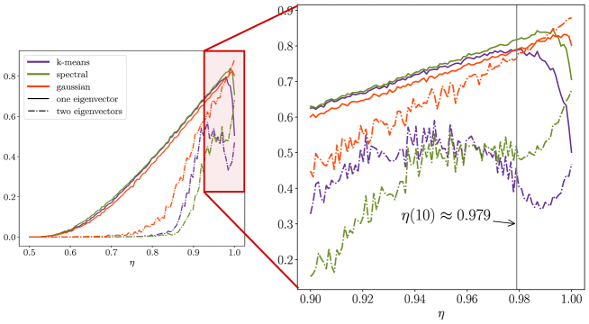
Figure 4: Top. Here $n=2000$, $s=10$ and $\eta=.99>\eta(10)=$, thus $r_{0}=2$. The Score is the adjusted overlap in (9).
Middle. For the two-block model with $\eta\in[0.5,1]$ we plotted the average Adjusted overlap over 100 runs of several clustering methods on spectral embeddings using either the embedding with the Perron vector $x\mapsto(u_{1}(x),0)$ (solid lines) or the embedding with two dominant eigenvectors $x\mapsto(u_{1}(x),u_{2}(x))$ (dashdot lines). In the inset we see that the performance of GMM is not reduced by the addition of the second informative eigenvector at the critical point $\eta(10)$.

In Figure 4, we performed some experiments regarding which clustering method to use on the spectral embedding. We simply used three popular methods, implemented in Python’s Sklearn library (Pedregosa et al. [2011]):

• k-means, the most popular method in graph clustering,

• Spectral-Clustering, which solves a norm-cut problem on the singular vectors of a distance matrix, a method known to be powerful when the clusters are non-convex,

• Gaussian Mixture clustering, which fits the parameters of a mixture of gaussians to the data using the E-M algorithm.

The first panel in Figure 4 is only a visual illustration of what spectral embeddings on a two-block SBM looks like. Here, the parameters are $\eta=0.99$ and $s=10$; our theory shows that there are two outliers in the spectrum of $A$. Our spectral embedding $\mathcal{X}$ in (7) has thus four dimensions (we use the left and right eigenvectors). For better visualization, we simply took the two right eigenvectors. Each point in the figure is thus $(u_{1}(x),u_{2}(x))$ for some node $x$ and the colors are the labels given by each clustering method.

The second panel in 4 shows the performance of these clustering methods, for $\eta$ between $1/2$ and $1$. We also compared the use of only one eigenvector with the use of two eigenvectors, even when there is only one informative eigenvector ($r_{0}=1$).

1. When there is only one outlier ($\eta<\eta(s)$), clustering based on the Perron eigenvectors (solid lines) yields good results, while adding a second uninformative eigenvector (dashdot lines) deeply reduces the performance of any clustering method.

2. When crossing $\eta(s)$, a second informative eigenvector appears; the performance of clustering methods based on the Perron eigenvector are reduced, in accordance with the correlation decrease of $|\langle u_{1},\varphi_{1}\rangle|$ predicted by Theorem 8 (see the golden line in Fig 1, first panel).

3. But, when $\eta>\eta(s)$, the performance of kmeans and spectral-clustering based on the two informative eigenvectors $u_{1},u_{2}$ first decreases, since these algorithms seem to struggle exploiting the extra information given by the second eigenvector (Figure 4, top panel). Only the Gaussian mixture model incorporates this extra information efficiently: it is the only method for which clustering based on two informative vectors is better than with only one (the two orange lines cross short after $\eta(s)$).

We did not try other clustering methods — these experiments are only indicative of a seemingly high performance for gaussian clustering. In Theorem 11, we showed that the spectral embeddings have a limiting distribution, accessible through the $Z_{i,j}$. If $Z_{i,j}$ was Gaussian, the performance of GMM would be completely understood, but as mentioned before Conjecture 12, in the sparse regime, the limiting distributions $Z_{i,j}$ (or equivalently, the spectral embeddings) are not Gaussian. The following remark explains why.

Remark 13.

$Z_{i,j}$ has a positive atom at $0$ (and possibly many other atoms): indeed, following the notations of the very last subsection, it is easily seen that the limit $\mathscr{Z}_{i,j}$ is equal zero when the Galton-Watson tree $\mathscr{T}_{j}$ is empty, which happens with strictly positive probability so $\mathbf{P}(Z_{i,j}>0)>0$; but clearly, the extinction probability of $\mathscr{T}_{j}$ goes to zero when $\nu_{1}$, the highest modularity eigenvalue, goes to infinity. Note that the atom at zero is visible in Figure 5-(a).

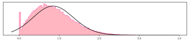
(a): $r_{0}=1$. Histogram of the entries of $u_{1}$.

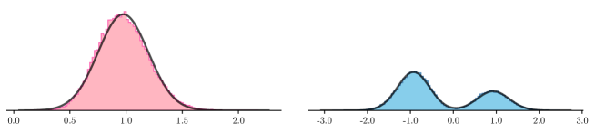
(b) $r_{0}=2$. Histogram of $u_{1}$ in pink, and $u_{2}$ in blue.

Figure 5: An illustration of Theorem 11, for the two-block SBM with connectivities as in (5) and clusters sizes $p_{1}=2/3,p_{2}=1/3$. Here, $n=5000$ and there are 10 samples in each picture. The grey lines are the densities of the gaussian mixtures in (11).

The shapes of the random variables $Z_{i,j}$ are visible in Figure 5. In this figure, we plotted the histograms of the entries of $u_{i}$ in two different $5000$-nodes blockmodels, with connectivies $F_{1}$ (top) and $F_{2}$ (bottom) given by:

$$F_{1} =\begin{pmatrix}6&4\\ 5&3\end{pmatrix} F_{2}=\begin{pmatrix}48&6\\ 12&24\end{pmatrix}$$ (10)

with two clusters of size $p_{1}=2/3,p_{2}=1/3$ — the same size on the left and on the right. In the first model, there is only one outlier; in the second, there are two.

Note that the Theorem implies that for $i\in[r_{0}]$, the densities of the discrete distributions

$$\frac{1}{n}\sum_{x\in[n]}\delta_{u_{i}(x)}$$

converge in distribution to $p_{1}Z_{i,1}+p_{2}Z_{i,2}$. The plots are the histograms of the $u_{i}(x)$ over 10 samples. In the figure, the grey lines are the densities of the gaussian mixtures

$$\mathcal{N}_{i}=p_{1}\mathscr{N}(\mu_{i,1},\sigma_{i,1}^{2})+p_{2}\mathscr{N}(\mu_{i,2},\sigma_{i,2}^{2}),$$ (11)

where $i\in\{1,2\}$ and $\mu_{i,j},\sigma_{i,j}^{2}$ are the means and variances of the limiting random variables $Z_{i,j}$. It is clearly seen that in the first plot, the limit of $u_{1}$ is not Gaussian; in the second plot, the degrees of the graph are much higher (we are already on the semi-sparse regime), and the Gaussian approximations for both eigenvectors are strikingly convincing.

Appendix B A bird’s eye view on the proof of Theorem 3

The proof of Theorem 3 follows the celebrated high-trace method, introduced in Massoulié [2014], Bordenave et al. [2018]. Considerable advances and simplifications have recently been made; on one hand, Stephan and Massoulié [2020] performed this method on the non-backtracking matrix of weighted, inhomogeneous undirected graphs; on the other hand, Bordenave et al. [2020] performed this method on the adjacency matrix of weighted, homogeneous directed graphs. In both of these papers, the underlying matrices $P$ and $W$ were Hermitian, which is no longer the case here. Our Master Theorem bridges the gap, and considers the adjacency matrix of weighted, inhomogeneous directed graphs with general $P,W$.

We hereby sketch the main ideas at a high level, and when needed we link our proof with the formerly cited papers. We emphasize that the proofs of theorems like Theorem 3 are often very technical. In this appendix, we tried to be as elementary as possible, to hide the technical details already written in other papers, and to give a short, accessible summary of the proof ideas — at the cost of completeness.

B.1 Warmup: notations

Probabilistic domination.

For readability, we introduce notations regarding the asymptotic order of real random variables. Let

$$X=(X_{n}:n\in\mathbb{N})\qquad\qquad Y=(Y_{n}:n\in\mathbb{N})$$

be two families of real random variables. We write $X\preceq Y$ if there is a constant $D$ such that for every constant $c>0$, for $n$ large enough,

$$\mathbb{P}(|X_{n}|>\log(n)^{D}|Y_{n}|)\leqslant\log(n)^{-c},$$

in other words, $|X_{n}|$ is smaller than $|Y_{n}|$ up to logarithmic terms, with probability smaller than every polylogarithm (typically, $n^{\delta}$ for small $\delta$). Finally, we write $X\ll Y$ if for every constants $c,D>0$, for $n$ large enough,

$$\mathbb{P}(|X_{n}|>\log(n)^{-D}|Y_{n}|)\leqslant\log(n)^{-c}.$$

In other words, $|X_{n}|/|Y_{n}|$ goes to zero faster than every polylogarithm. With this handy device, it is easily seen that $X_{n}\preceq Y_{n}$ and $Y_{n}\ll Z_{n}$ imply $X_{n}\ll Z_{n}$. These notations are common in the field of random matrix theory, and they truly simplify the exposition compared with Stephan and Massoulié [2020], Bordenave et al. [2020].

Spectral decomposition.

Before starting, we write the spectral decomposition of $Q=\mathbf{E}[A]$:

$$Q=\sum_{i=1}^{r}\mu_{i}\varphi_{i}\psi_{i}^{*}.$$

The $\mu_{i}$ are the $r$ nonzero eigenvalues; we order them by decreasing modulus, $|\mu_{1}|>\dotsb>|\mu_{r}|$. The $\varphi_{i}$ are the corresponding unit right eigenvectors; they do not always an orthonormal basis, because $Q$ has not been supposed normal. The $\psi_{i}$ are the unique (up to a sign) left eigenvectors satisfying $\langle\varphi_{i},\psi_{j}\rangle=\delta_{i,j}$, and in general they do not have unit-length. In the statement of the Master Theorem, the unit left eigenvectors $\xi_{i}$ are thus $\psi_{i}/|\psi_{i}|$.

Thresholds, spectral gap.

We recall that $r_{0}$ is the number of eigenvalues of $Q$ with modulus greater than $\upvartheta=\max(\|W\|_{\infty},\sqrt{\rho})$ where $\rho=\sqrt{\|K\|}$ and we introduce $\Phi=(\varphi_{1},\dotsc,\varphi_{r_{0}}),\Psi=(\psi_{1},\dotsc,\psi_{r_{0}})$ and $\Sigma=\mathrm{diag}(\mu_{1},\dotsc,\mu_{r_{0}})$. The spectral gap of our model is defined as

$$\tau=\sqrt{\frac{\upvartheta}{|\mu_{r_{0}}|}}.$$

It is very important to note that $\tau<1$. The closer to $1$, the harder the problem; the bounds of Theorem 3 are actually of the form $\left|\lambda_{i}-\mu_{i}\right|\preceq\tau^{\ell}$, where $\ell$ is a carefully chosen parameter that grows logarithmically with $n$.

Covariance functionals, eigendefects and cross-defects

We will first need a notation for the Hadamard products of vectors in $\mathbb{R}^{n}$:

$$\varphi^{i,j}=\varphi_{i}\odot\varphi_{j}\qquad\text{ and }\qquad\psi^{i,j}=\psi_{i}\odot\psi_{j},$$ (12)

so that in the statement of the Master Theorem, $\varphi_{i}^{2}$ is equal to $\varphi^{i,i}$. In the proof we will only use the $\varphi^{i,i}$ notation.

We introduce two functions $\Gamma,\Gamma^{*}:\mathbb{C}\times\mathbb{C}^{n}\to\mathbb{C}$ by

$$\Gamma(z,\xi)=\sum_{t=0}^{\infty}\frac{\langle\mathbf{1},K^{t}\xi\rangle}{z^{t}}\qquad\text{ and }\qquad\Gamma^{*}(z,\xi)=\sum_{t=0}^{\infty}\frac{\langle\mathbf{1},(K^{*})^{t}\xi\rangle}{z^{t}}.$$ (13)

Let us recall that the norm of $K$ is $\rho$; consequently, the sums above are convergent when $|z|$ is strictly greater than $\rho$, and in particular when $z=\mu_{i}^{2}$ with $i\in[r_{0}]$. In this case, one has

$$\Gamma(\mu_{i}^{2},\varphi^{i,i})=\mu_{i}^{2}\sqrt{R_{i}}\qquad\text{ and }\qquad\Gamma^{*}(\mu_{i}^{2},\psi^{i,i})=\mu_{i}^{2}\sqrt{L_{i}}.$$ (14)

Proof.

Let $\xi=\varphi^{i,i}$. We have $\Gamma(\mu_{i}^{2},\xi)=\sum_{t=0}^{\infty}\frac{\langle\mathbf{1},K^{t}\xi\rangle}{\mu_{i}^{2t}}=\langle\mathbf{1},(\sum_{t=0}^{\infty}(K/\mu_{i}^{2})^{t})\xi\rangle$. The Neumann summation formula shows that since $\|K/\mu_{i}^{2}\|<1$, the matrix sum in this expression is nothing but $(I-K/\mu_{i}^{2})^{-1}=\mu_{i}^{2}(\mu_{i}^{2}I-K)^{-1}$, and that this matrix has all entries nonnegative. Since $\xi$ also has nonnegative entries, $|(\mu_{i}^{2}I-K)^{-1}\xi|_{1}=\langle\mathbf{1},(\mu_{i}^{2}I-K)^{-1}\xi\rangle$, and we recognize the right eigendefects. ∎

Since we’ll also need ‘cross defects’ like $\Gamma(\mu_{i}\mu_{j},\varphi^{i,j})$, we introduce the notations $\Gamma_{\mathrm{left}},\Gamma_{\mathrm{right}}$ for two matrices of size $r_{0}\times r_{0}$ defined by

$$(\Gamma_{\mathrm{left}})_{i,j}=\Gamma(\mu_{i}\mu_{j},\varphi^{i,j})\qquad\text{ and }\qquad(\Gamma_{\mathrm{right}})_{i,j}=\Gamma^{*}(\mu_{i}\mu_{j},\psi^{i,j}).$$

B.2 The Pseudo-Master Theorem: $A$ is nearly diagonalized by pseudo-eigenvectors

The tools for studying matrix $A$ are the pseudo-eigenvectors. Consider the eigenvalue $\mu_{i}$ of $Q$. We define two vectors $U_{i}=A^{\ell}\varphi_{i}/\mu_{i}^{\ell}$ and $V_{i}=(A^{*})^{\ell}\psi_{i}/\mu_{i}^{\ell}$, where

$$\ell=\lfloor\kappa\log(n)\rfloor$$ (15)

and $\kappa$ is a positive constant to be chosen later. To put it in matrix form, these vectors are the columns of the $n\times r_{0}$ matrices

$$U=A^{\ell}\Phi\Sigma^{-\ell}\qquad\text{ and }\qquad V=(A^{*})^{\ell}\Psi\Sigma^{-\ell}.$$

The key aspects of $U$ and $V$ are summarized in the following list of statements, which is a pseudo-version of the Master Theorem. We recall that the symbols $\ll,\preceq$ where rigorously defined in the preceding subsection.

Theorem 14 (Pseudo-Master Theorem).

For a sufficiently small choice of $\kappa$, the following holds.

1. $U$ and $V$ are nearly inverses:

   $$\|U^{*}V-I\|\ll 1$$ (16)

2. $U$ and $\Psi$ are nearly inverses, and $V$ and $\Phi$ are nearly inverses:

   $$\|\Psi^{*}U-I\|\ll 1\qquad\qquad\|\Phi^{*}V-I\|\ll 1$$ (17)

3. $V$ and $U$ nearly diagonalize $A^{\ell}$:

   $$\|V^{*}A^{\ell}U-\Sigma^{\ell}\|\ll 1$$ (18)

4. $\Gamma_{\mathrm{left}}$ is nearly the Gram matrix of $U$, and the same for $\Gamma_{\mathrm{right}}$ and $V$:

   $$\|U^{*}U-\Gamma_{\mathrm{left}}\|\ll 1\qquad\qquad\|V^{*}V-\Gamma_{\mathrm{right}}\|\ll 1$$ (19)

5. $A^{\ell}$ is negligible outside of the vector spaces spanned by the pseudo-eigenvectors:

   $$\|A^{\ell}\mathrm{Proj}_{\mathrm{im}(V)^{\perp}}\|\preceq\upvartheta^{\ell},\qquad\qquad\|\mathrm{Proj}_{\mathrm{im}(U)^{\perp}}A^{\ell}\|\preceq\upvartheta^{\ell},$$ (20)

   where $\mathrm{Proj}_{C^{\perp}}$ denotes the projection matrix on the orthocomplement of the subspace $C$.

A crucial point in this theorem is that the error scale (up to polylog factors) is $\upvartheta$: only the last bound, (20), is actually sharp. The other error terms are meant to be negligible.

Proving the Pseudo-Master Theorem (PMT) is really the core of the proof, and where lie most of the difficulties. From the PMT, it is only a matter of linear algebra and perturbation theory to prove the Master Theorem: we simply summarize the spirit in the next subsection, and we quickly jump to the proof of the PMT.

B.3 Master Theorem = Pseudo-Master Theorem + perturbation theory

Given the statements in the preceding subsection, the main theorem follows from a standard algebraic analysis, which builds on detailed quantitative variants of the Bauer-Fike theorem. We refer the reader to the comprehensive studies in [Stephan and Massoulié, 2020, Section 4] or [Bordenave et al., 2020, Section 8], which are technical, but can be applied directly without any further modification. In this short paragraph, we simply explain the ideas.

The main trick is to define a matrix $S=U\Sigma^{\ell}V^{*}$. If we had $V^{*}U=I$, this matrix would be exactly diagonalizable with eigenvalues $\mu_{i}^{\ell}$; but $V^{*}U$ is only close to $I$. Fortunately, it is easily seen that if $U,V$ are well-conditioned, then $S$ is diagonalizable, with eigenvalues close to the $\mu_{i}^{\ell}$ and eigenvectors close to the $U_{i},V_{j}$. The fact that $U,V$ are well-conditioned follows from (19): by continuity, their condition number is close to the condition number of $\Gamma_{\mathrm{right}},\Gamma_{\mathrm{left}}$, who in turn are bounded:

Lemma 15.

The condition numbers of the matrices $\Gamma_{\mathrm{right}},\Gamma_{\mathrm{left}},U,V$ are all $\preceq 1$.

Proof.

Note $\pi_{s}(x)=\sqrt{(K^{*})^{s}\mathbf{1}(x)}$ and $\Pi_{s}=\mathrm{diag}(\pi_{s})$. It is easily seen that $\langle\mathbf{1},K^{s}\varphi^{i,j}\rangle=(\Phi^{*}\Pi^{2}_{s}\Phi)_{i,j}$. The matrix $\Gamma_{\mathrm{left}}$ is thus a sum of semi-definite positive matrices, with first term $I_{0}$, so its smallest eigenvalue is $\geqslant 1$ and its condition number is smaller than $\|\Gamma_{\mathrm{left}}\|$. On the other hand, note that $|\langle\mathbf{1},K^{s}\varphi^{i,j}\rangle|\leqslant|\mathbf{1}||\varphi^{i,j}|\rho^{s}$. Thanks to (2), we have $|\varphi^{i,j}|\leqslant c\sqrt{1/n}$ for some $c$; consequently, $(\Gamma_{\mathrm{left}})_{i,j}\leqslant c\sum\rho^{s}/(\mu_{i}\mu_{j})^{s}\leqslant c/(1-\tau)\preceq 1$. Finally, since the size $r_{0}$ is also $\preceq 1$, we have $\|\Gamma_{\mathrm{left}}\|\preceq 1$ and the condition number is $\preceq 1$. By the Weyl inequalities and (19), $|\mathrm{cond}(U)-\mathrm{cond}(\Gamma_{\mathrm{left}})|\leqslant\|UU^{*}-\Gamma_{\mathrm{left}}\|\ll 1$ and $\mathrm{cond}(U)\preceq 1$. ∎

The smallest eigenvalue $\nu_{r_{0}}$ of $S$ is close to $\mu_{r_{0}}^{\ell}$, and since $\tau>1$ independently of $n$ and $\ell=\lfloor\kappa\log(n)\rfloor$, we get $|\mu_{r_{0}}^{\ell}|\ll\upvartheta^{\ell}$. But we can write $A^{\ell}$ as a perturbation of $S$,

$$A^{\ell}=S+(A^{\ell}-S),$$

and, crucially, statements (18)-(20) can be bootstraped to show that $\|A^{\ell}-S\|\ll 1$. The Bauer-Fike theorem applies, and roughly says that the eigenvalues of $A^{\ell}$ are within distance $\ll\upvartheta^{\ell}$ of the eigenvalues of $S$: consequently, $A^{\ell}$ has $r_{0}$ eigenvalues $\upvartheta^{\ell}$-close to $\mu^{\ell}_{1},\dotsc,\mu_{r_{0}}^{\ell}$, and the eigenvalue $0$ of $S$ gives rise to $n-r_{0}$ eigenvalues of $A^{\ell}$ with modulus $\preceq\upvartheta^{\ell}$. A similar statement holds for the eigenvectors; extra work needs to be done for getting results on the eigenvalues of $A$, since there might be some phase effects.

The results on eigenvectors follow in the same way, with a Davis-Kahan-like custom theorem proved in Stephan and Massoulié [2020]. To ensure performant bounds, we must assume that the eigenvalues $\mu_{i}$ are well-separated, which the reason why we suppose that $|\mu_{i}-\mu_{j}|>c$ for some $c>0$ in the Hypotheses before the Master Theorem. Since $\|A^{\ell}-S\|\ll 1$ and the condition numbers of the matrices of interest are all $\preceq 1$, the Davis-Kahan theorem yields a bound of the form $|u_{i}-U_{i}/|U_{i}||\preceq\|A^{\ell}-S\|/c$, which is $\ll 1$:

$$\left|u_{i}-\frac{U_{i}}{|U_{i}|}\right|\ll 1.$$ (21)

The ‘eigenvector part’ of the Master Theorem then easily follows, by the continuity of $u\mapsto\langle u,\varphi\rangle$ and the limits in the Pseudo-Master Theorem.

Appendix C Proof of the Pseudo-Master Theorem

This section is devoted to the proof of the Pseudo-Master Theorem.

The first two sections gather some results on local approximations of random graphs: to a large extent, they are classical and well-known. We state them for completeness and because they give a good intuition on the following parts, but these statements can be retrieved using routine methods from random graph theory. Subsection C.3 states a powerful concentration result on random graphs, proved in Bordenave et al. [2020].

We use these results as a computational toolbox: in Subsections C.4 to C.7, we perform all the necessary calculations on our pseudo-eigenvectors, and we rely on an elegant generalization of Kesten martingales on inhomogeneous Galton-Watson trees. These sections differ from previous works in the sense that we had to adapt the computations to the general setting of our Master Theorem, with full inhomogeneity and non-symmetry.

Finally, the main ideas of previous works on trace methods are summarized in Subsection C.8, as they apply without modifications to our setting.

C.1 The graph has few short cycles, and small neighbourhood growth

Sparse random graphs, that is, random graphs where the mean degree of vertices is $O(1)$, have been known for long to be locally-tree like, in the sense they have very few short cycles. In our model, we supposed that $P_{x,y}\leqslant d/n$ for some $d$. As a consequence, the expected degree of a vertex $x$ is $d_{x}=P_{x,1}+\dotsb+P_{x,n}$, and is smaller than $d$, and the graph is stochastically dominated by a directed homogeneous Erdős-Rényi random graph with connectivity $d/n$. In turn, many random variables (cycle counts, edge number) are stochastically dominated by the undirected Erdős-Rényi graph of degree $2d/n$. Most properties on the local structure directly follow from classical results: absolutely no problem-specific work is needed here. We simply gather the results we will tacitly use in the sequel.

We note $(G,x)_{t}$ the forward neighbourhood of radius $t$ around $x$ in $G$, that is: the subgraph spanned by vertices $y$, for which there is a directed path with length smaller than $t$ from $x$ to $y$. The crucial choice will be the depth $\ell$ at which we look into the graph. We recall

$$\ell=\lfloor\kappa\log(n)\rfloor$$

where $\kappa$ is an explicit constant depending on $d$. With such a choice, we have the crucial property that shallow neighborhoods are nearly trees. We say that a graph is $t$-tangle-free if for every vertex $x$, the subgraph $(G,x)_{t}$ has no more than one directed cycle.

Lemma 16.

There is a constant $c=c(d)$ such that $G$ is $2\ell$-tangle-free with probability $\geqslant 1-n^{-c}$. Moreover, if $N$ is the number of vertices $x$ such that $(G,x)_{2\ell}$ contains a cycle, then $N\preceq 1$.

The proof Lemma 16 follow from the choice of the constant $\kappa$ in (C.1). We refer to [Bordenave et al., 2018] for the details.

C.2 The graph is locally approximated by trees

Let $x$ be a vertex in $G$, and $\mathcal{N}(x)$ the set of its neighbours (in the forward sense: $y$ is a neighbor or $x$ if $(x,y)\in E$, not necessarily when $(y,x)\in E$). Then $\mathcal{N}(x)$ has the following distribution : each vertex $y\neq x$ is present in $\mathcal{N}(x)$ with probability $P_{x,y}$, independently from all other vertices. It is a well-known fact that whenever the $P_{x,y}$ are small, the law of $|\mathcal{N}(x)|$ is well approximated by $\mathrm{Poi}(d_{x})$ (the so-called ‘rare events theorem’). Moreover, conditionnally on $\{\mathcal{N}(x)\neq\varnothing\}$, the distribution of a random element in $\mathcal{N}(x)$ is equal to $\pi_{x}$, where

$$(\pi_{x})_{z}=P_{x,z}/d_{x}.$$ (22)

That being said, the distribution of $k$ elements in $\mathcal{N}(x)$ is not the product distribution $(\pi_{x})^{\otimes k}$ because the elements have dependencies (they cannot be chosen multiple times, for instance), but these dependencies are nearly nonexistent. In fact, let us introduce a new distribution $\mathbb{Q}_{x}$ on random multi-sets.

• The number of elements of the random multiset $\mathcal{M}(x)$ under $\mathbb{Q}_{x}$ is a Poisson random variable with mean $d_{x}$;

• Conditionnally on $|\mathcal{M}(x)|=k$, each of these $k$ element is sampled independently on $[n]$ with probability distribution $\pi_{x}$.

The following proposition is a rigorous formulation of the intuitions given above. We set $\sigma_{x}=P^{2}_{x,1}+\dotsb+P^{2}_{x,n}$; in our regime, $\sigma_{x}=O(1/n)=o(1)$.

Proposition 17.

[Stephan and Massoulié, 2020, Lemma 8] We have

$$d_{\mathrm{TV}}(\mathbb{P}_{x},\mathbb{Q}_{x})\leqslant 2\sigma_{x}.$$ (23)

Building from those remarks, we define a random tree $T_{x}$ as follows :

• the root (at depth $0$) is a single vertex labeled $x$,

• for each vertex $i$ at depth $t$ with label $x_{i}$, the children of $i$ at depth $t+1$ with their labels have the joint distribution $\mathcal{M}(x_{i})$, independently from all other vertices at depth $\leqslant t$.

With this definition, the tree $T_{x}$ is formally undirected, but we can view it as a directed tree with directions flowing out of the root. Proposition 17 then implies that the neighbourhood distributions in $T_{x}$ and $G$ are similar, as summarized in the following result:

Lemma 18.

Whenever $\ell=\lfloor\kappa\log(n)\rfloor$ with $\kappa$ small enough, we have

$$d_{\mathrm{TV}}((G,x)_{2\ell},(T_{x},x)_{2\ell})\ll 1.$$ (24)

This lemma will not directly be used in our proof; it is only a step in the proof of Proposition 19 thereafter. We stated it anyways because it gives a rigorous meaning to the fact that $G$ is well-approximated locally by trees, and it intuitively gives a justification for our tree computations in subsequent parts of the proofs.

Note that we formulated this section only with forward neighborhoods; the propositions are also true with backward neighborhoods, and in this case we only have to see $T_{x}$ as a directed tree, with edges oriented towards the root.

C.3 Concentration of linear functionals

The graph $G$ (or the matrix $A$) is a collection of $n^{2}$ independent random variables: it is thus natural that if $F(G,x)$ is a function which depends only on a small neighborhood of the graph, then its space average

$$\frac{1}{n}\sum_{x\in[n]}F(G,x)$$ (25)

should be concentrated around its mean. This is the case, and a stronger statement actually holds: we saw in (24) that $(G,x)$ and $(T_{x},x)$ nearly have the same distribution, and it is actually known that the functional in (25) is indeed concentrated around the expectation of the same functional applied on the trees $(T_{x},x)$.

To formalize this, we say that a function $f:\mathscr{G}\times\mathbb{N}\mapsto\mathbb{R}$, where $\mathscr{G}$ denotes the set of all graphs, is $\ell$-local if $f(H,x)$ only depends on the $\ell$-neighbourhood of $x$ in $H$. Let $(T_{x},x)$ be the family of independent random rooted trees as in (24). Then the following lemma is true as long as the constant $\kappa$ in $\ell$ is small enough ($\kappa<0.01/\log(2d)$ will be sufficient).

Proposition 19.

Let $\mathscr{F}$ be a family of functions $f:\mathscr{G}\times\mathbb{N}\mapsto\mathbb{R}$, with less than $\preceq 1$ elements. We suppose that each $f\in\mathscr{F}$ is a $2\ell$-local function, that for all graphs $H$ and node $x$ one has $\sup_{f\in\mathscr{F}}f(H,x)\leqslant|(H,x)_{2\ell}|^{2}\times(c_{n}/n)$, for some $c_{n}>0$. Then

$$\sup_{f\in\mathscr{F}}\left|\sum_{x\in G}f(G,x)-\sum_{x\in[n]}\mathbf{E}\left[f(T_{x},x)\right]\right|\preceq\frac{c_{n}}{n^{0.1}}.$$

Proof.

This is a restatement of Theorem 12.5 in Bordenave et al. [2020], with $\beta=2$ and $\alpha=c_{n}/n$. The bound therein is $c_{n}n^{-1/2+2\kappa}$. A sufficiently small $\kappa$ leads to our statement. Note that if $f(H,x)\leqslant|(H,x)_{2\ell}|$, then $f$ also satisfies $f(H,x)\leqslant|(H,x)_{2\ell}|^{2}$, which is the reason why we chose to keep the exponent $2$. ∎

A crucial point in the proof of the Pseudo-Master Theorem is that the pseudo-eigenvectors $U_{i}$ and $V_{i}$ are $\ell$-local functions of $G$, and thus so are their scalar products with one another. As such, all computations in (16)-(18) reduce to computing expectations on the random trees defined in the preceding subsection. We can apply Lemma 19 to $G$ and the family $(T_{x})_{x}$; the problem was reduced to computing the expectations of our functionals on the trees $T_{x}$.

C.4 Pseudo-eigenvectors on the random tree

Let us take a quick look at the entries of $U$ and $V$, and pick one vertex $x\in[n]$ and some index $i$. By definition,

$$U_{i}(x) =\mu_{i}^{-\ell}(A^{\ell}\varphi_{i})(x)$$

$$=\mu_{i}^{-\ell}\sum_{x_{1},\dotsc,x_{\ell}}W_{x,x_{1}}W_{x_{1},x_{2}}\dotsb W_{x_{\ell-1},x_{\ell}}\varphi_{i}(x_{\ell}),$$ (26)

where the sum runs over all the paths in the graph $G$, ie sequences of vertices such that the edges $(x_{s},x_{s+1})$ are present in the graph.

This is, by definition, an $\ell$-local function ; its counterpart on the tree can thus be defined as

$$\tilde{U}_{i}(x)=\mu_{i}^{-\ell}\sum_{x_{1},\dots,x_{\ell}\in T_{x}}W_{x,\iota(x_{1})}W_{\iota(x_{1}),\iota(x_{2})}\dotsb W_{\iota(x_{\ell-1}),\iota(x_{\ell})}\varphi_{i}(\iota(x_{\ell})),$$ (27)

where the sum ranges over the vertices $x_{\ell}$ at depth $\ell$ in $T_{x}$ and the unique path $x,\dots,x_{\ell}$ connecting $x$ to $x_{\ell}$, and $\iota(x_{i})$ is the label of $x_{i}$.

C.5 The martingale equation

Let $\mathbf{E}_{\ell-1}$ denote the conditional expectation with respect to the first $\ell-1$ generations of $T_{x}$. Write

$$\mathbf{E}_{\ell-1}[\tilde{U}_{i}(x)]=\mu_{i}^{-\ell}\sum_{x_{1},\dotsc,x_{\ell-1}}W_{x,\iota(x_{1})}\dotsb W_{\iota(x_{\ell-2}),\iota(x_{\ell-1})}\mathbf{E}_{\ell-1}\left[\sum_{x_{\ell}}W_{\iota(x_{\ell-1}),\iota(x_{\ell})}\varphi_{i}(\iota(x_{\ell}))\right].$$

Let us note $y=\iota(x_{\ell-1})$; the inner expectation reads

$$\mathbf{E}_{\ell-1}\left[\sum_{x_{\ell}}W_{\iota(x_{\ell-1}),\iota(x_{\ell})}\varphi_{i}(\iota(x_{\ell}))\right]=\mathbf{E}\left[\sum_{z\in\mathcal{M}(y)}W_{y,z}\varphi_{i}(z)\right]$$

This is a sum of a $\mathrm{Poi}(d_{y})$ number of independent random variables with distribution $\pi_{y}$, so

$$\mathbf{E}\left[\sum_{z\in\mathcal{M}(y)}W_{y,z}\varphi_{i}(z)\right] =d_{y}\times\sum_{z\in[n]}\frac{P_{y,z}}{d_{y}}W_{y,z}\varphi_{i}(z)$$

$$=\sum_{y\in[n]}P_{y,z}W_{y,z}\varphi_{i}(z)$$

$$=\sum_{y\in[n]}Q_{y,z}\varphi_{i}(z)$$

$$=(Q\varphi_{i})(y)$$

$$=\mu_{i}\varphi_{i}(y)$$

where, in the last line, we used the fact the $\varphi_{i}$ is an eigenvector of $Q$. Recalling that $y=\iota(x_{\ell-1})$, we have

$$\mathbf{E}_{\ell-1}[\tilde{U}_{i}(x)]=\mu_{i}^{-\ell+1}\sum_{x_{1},\dotsc,x_{\ell-1}}W_{x,\iota(x_{1})}\dotsb W_{\iota(x_{\ell-2}),\iota(x_{\ell-1})}\varphi_{i}(\iota(x_{\ell-1})).$$

In fact, defining $\tilde{U}_{i}(x,t)$ by replacing $\ell$ by $t$ in the definition of $\tilde{U}_{i}(x)$, we showed that

$$\text{The random process }t\mapsto\tilde{U}_{i}(x,t)\text{ is a martingale}.$$ (28)

The common expectation is easily seen to be $\mathbf{E}[\tilde{U}_{i}(x,0)]=\varphi_{i}(x)$.

C.6 Proving (16)-(17)-(18)

We only give the argument for (16), the others are done in a similar fashion. The $(i,j)$ coefficient of $U^{*}V$ is $\langle U_{i},V_{j}\rangle$, which can be rewritten as

$$\langle U_{i},V_{j}\rangle=(\mu_{i}\mu_{j})^{-\ell}\langle A^{\ell}\varphi_{i},(A^{*})^{\ell}\psi_{j}\rangle=(\mu_{i}\mu_{j})^{-\ell}\langle A^{2\ell}\varphi_{i},\psi_{j}\rangle$$

Let $f(x)=f_{i,j}(x)=\psi_{j}(x)[A^{2\ell}\varphi_{i}](x)$; it is easily seen that $\langle U_{i},V_{i}\rangle=\sum_{x\in[n]}f(G,x)$, and we are ready to apply the concentration property in Proposition 19 to the family $\{f_{i,j}\}$.

Lemma 20 (correlations between pseudo-eigenvectors are concentrated).

$$\sup_{i,j}\left|\langle U_{i},V_{j}\rangle-\mu_{i}^{-\ell}\mu_{j}^{-\ell}\sum_{x\in[n]}\psi_{j}(x)\mathbf{E}[\tilde{U}_{i}(x,2\ell)]\right|\ll 1$$ (29)

Proof.

The delocalization properties of the $\varphi_{i}$ (Hypothesis (2)), the tangle-free property (there is no more than one cycle in $(G,x)$) and the fact that $|W_{x,y}|\leqslant\|W\|_{\infty}$ all together imply that

$$f(G,x)\leqslant\frac{c\|W\|^{\ell}_{\infty}}{n}|(G,x)_{2\ell}|,$$

for some universal constant $c$. But since $\|W\|_{\infty}<c^{\prime}$ for some $c^{\prime}$, any choice for $\kappa$ sufficiently small will give (for instance) $\|W\|_{\infty}^{\ell}\preceq n^{0.01}$. Proposition 19 straightforwardly leads to a $\preceq n^{-\varepsilon}$ error for some small $\varepsilon$. With our notations, this is $\ll 1$.

∎

We are now in a position to use property (28): $\mathbf{E}[\tilde{U}_{i}(x,2\ell)]=\varphi_{i}(x)$, and the orthogonality property of the left and right eigenvectors yields $\left|\langle U_{i},V_{j}\rangle-\delta_{ij}\right|\ll 1$. It is then straightforward to go from this elementwise bound to (16): for any $r_{0}\times r_{0}$ matrix $M$, one has $\|M\|\leqslant r\|M\|_{\infty}$. Since we also have $r\preceq 1$, we obtain $\|U^{*}V-I\|\preceq\|U^{*}V-I\|_{\infty}\ll 1$.

The same proof works for $V$, with the subtle difference that these left-pseudo-eigenvectors $V_{i}$ are backward-looking: $V_{i}(x)$ is a local function of $(G,x)_{\ell}^{-}$, where the $-$ superscript denotes the backward ball. But the proof is the same: Lemma 19 is true for backward functionals and the couplings in Subsection C.2 are the same, but with the $T_{x}$ oriented towards the root; everything works exactly the same.

C.7 Proving (19): martingale correlations

Statements in (19) are trickier: even if Lemma 19 still allows approximating $\langle U_{i},U_{j}\rangle$ with a tree computation, there are some strong dependencies between $\tilde{U}_{i}(x,t)$ and $\tilde{U}_{j}(x,t)$ that we cannot neglect.

Rewriting the correlation term.

Proceeding as before with $f(G,x)=[A^{\ell}\varphi_{i}](x)\cdot[A^{\ell}\varphi_{j}](x)$, we have

$$\sup_{i,j}\left|\langle U_{i},U_{j}\rangle-\sum_{x\in[n]}\mathbf{E}\left[\tilde{U}_{i}(x)\tilde{U}_{j}(x)\right]\right|\ll 1.$$ (30)

We recognize a covariance term between two martingales; let us then introduce the increments

$$\Delta_{t}=\mathbf{E}_{t-1}\left[(\tilde{U}_{i}(x,t)-\tilde{U}_{i}(x,t-1))(\tilde{U}_{j}(x,t)-\tilde{U}_{j}(x,t-1))\right]$$

A classical use of the martingale property implies that

$$\mathbf{E}\left[\tilde{U}_{i}(x)\tilde{U}_{j}(x)\right]=\varphi_{i}(x)\varphi_{j}(x)+\mathbf{E}[\Delta_{1}+\dots+\Delta_{\ell}]$$

The increment $\Delta_{t}$ has an explicit expression:

$$\Delta_{t}=\mu_{i}^{-t}\mu_{j}^{-t}\sum_{\begin{subarray}{c}x_{1},\dotsc,x_{t-1}\\ x^{\prime}_{1},\dotsc,x^{\prime}_{t-1}\end{subarray}}\prod_{s=1}^{t-1}W_{\iota(x_{s-1}),\iota(x_{s})}W_{\iota(x^{\prime}_{s-1}),\iota(x^{\prime}_{s})}\times\\ \mathbf{E}_{t-1}\left[\sum_{\begin{subarray}{c}x_{t-1}\to x_{t}\\ x^{\prime}_{t-1}\to x^{\prime}_{t}\end{subarray}}W_{\iota(x_{t-1}),\iota(x_{t})}W_{\iota(x^{\prime}_{t-1}),\iota(x^{\prime}_{t})}\varphi_{i}(\iota(x_{t}))\varphi_{j}(\iota(x^{\prime}_{t}))-\mu_{i}\mu_{j}\varphi_{i}(\iota(x_{t-1}))\varphi_{j}(\iota(x^{\prime}_{t-1}))\right].$$ (31)

Covariance of Poisson sums.

In the sum above, the only nonzero terms are when $x_{t-1}=x_{t-1}^{\prime}$: otherwise, the inner sum becomes a product of two independent random variables of respective expectations $\mu_{i}\varphi_{i}(x_{t-1})$ and $\mu_{j}\varphi_{j}(x_{t-1}^{\prime})$. Writing again $y=\iota(x_{t-1})$, the conditional expectation becomes

$$\begin{split}C_{y}:&=\mathbf{E}\left[\sum_{z,z^{\prime}\in\mathcal{M}(y)}W_{y,z}W_{y,z^{\prime}}\varphi_{i}(z)\varphi_{j}(z^{\prime})-\mu_{i}\mu_{j}\varphi_{i}(y)\varphi_{j}(y)\right]\\ &=\mathrm{Cov}\left(\sum_{z\in\mathcal{M}(y)}W_{y,z}\varphi_{i}(z),\sum_{z\in\mathcal{M}(y)}W_{y,z}\varphi_{j}(z)\right).\end{split}$$ (32)

We then make use of the following elementary lemma:

Lemma 21.

If $N$ is a Poisson random variable and $(A_{1},B_{1}),(A_{2},B_{2}),\dotsc$ are iid copies of a couple of random variable $(A,B)$, then

$$\mathrm{Cov}\left(\sum_{k=1}^{N}A_{k},\sum_{k=1}^{N}B_{k}\right)=\mathbf{E}[N]\mathbf{E}[AB].$$ (33)

In (32), $N=|\mathcal{M}(y)|$ is a $\mathrm{Poi}(d_{y})$ random variable, and the couple $(A,B)$ is simply

$$A=W_{y,Z}\varphi_{i}(Z)\qquad\text{and}\qquad B=W_{y,Z}\varphi_{j}(Z),$$

where $Z$ is a random index on $[n]$ with distribution $\pi_{y}$. Computing $C_{y}$ is now straightforward:

$$C_{y} =d_{y}\mathbf{E}[W_{y,Z}\varphi_{i}(Z)W_{y,Z}\varphi_{j}(Z)]$$

$$=d_{y}\sum_{z\in[n]}\frac{P_{yz}}{d_{y}}W_{yz}^{2}\varphi_{i}(z)\varphi_{j}(z)$$

$$=(K\varphi^{i,j})(y).$$

Let us now come back to (31). We know that we can remove every term with $x_{t-1}\neq x_{t-1}^{\prime}$, and the computations above further reduce it to

$$\Delta_{t}=(\mu_{i}\mu_{j})^{-t}\sum_{x_{1},\dots,x_{t-1}}\prod_{s=1}^{t-1}W_{\iota(x_{s-1},\iota(x_{s}))}^{2}(K\varphi^{i,j})(\iota(x_{t-1}))$$

We recognize an expression similar to the definition of $\tilde{U}_{i}$ in (27). Using the same methods, we are able to show that

$$\mathbf{E}[\Delta_{t}]=\frac{[K^{t}\varphi^{i,j}(x)]}{(\mu_{i}\mu_{j})^{t}}.$$

Finally, summing the increments, we get

$$\mathbf{E}[\tilde{U}_{i}(x)\tilde{U}_{j}(x)] =\varphi_{i}(x)\varphi_{j}(x)+\sum_{t=1}^{\ell}K^{t}\varphi^{i,j}(x)$$

$$=\sum_{t=0}^{\ell}\frac{K^{t}\varphi^{i,j}(x)}{\mu_{i}^{t}\mu_{j}^{t}}.$$ (34)

The expression for $\langle U_{i},U_{j}\rangle$ is obtained by summing (34) over all values of $x$ and plugging this into (19), thus obtaining:

$$\sup_{i,j}\left|\langle U_{i},U_{j}\rangle-\sum_{t=0}^{\ell}\frac{\langle\mathbf{1},K^{t}\varphi^{i,j}\rangle}{(\mu_{i}\mu_{j})^{t}}\right|\ll\upvartheta^{\ell}.$$ (35)

Statement (35) is pretty close to (19), at the sole difference of the summation index, which is stopped at $\ell$. Also, note that (35) is valid for every $i,j$ in $[r]$, not just in $[r_{0}]$. However, whenever $i,j\in[r_{0}]$, we have by definition

$$\sqrt{\rho}\leqslant\sqrt{\tau}\mu_{i}\quad\text{and}\quad\sqrt{\rho}\leqslant\sqrt{\tau}\mu_{j},$$

and the spectral radius of the matrix $K/(\mu_{i}\mu_{j})$ is thus at most $\tau$. Since the entries of $\varphi^{i,j}$ are of order $O(n^{-1})$, we have the bound

$$\sup_{i,j}\left|\sum_{t=\ell+1}^{\infty}\frac{\langle\mathbf{1},K^{t}\varphi^{i,j}\rangle}{(\mu_{i}\mu_{j})^{t}}\right|\leqslant C\tau^{\ell}\ll 1.$$

Combined with (35), this finally ends the proof of (19).

C.8 The trace method

All that remains now is to prove equation (20); that is, once we showed that the first $r_{0}$ eigenvalues of $A^{\ell}$ are close to the $\mu_{i}^{\ell}$, it remains to show that the $n-r_{0}$ eigenvalues are confined in a circle of radius $\upvartheta^{\ell}$. This is done in three parts:

1. a tangle-free decomposition, expressing $A^{\ell}$ as a product involving its expectation $Q$, the powers $A^{t}$ for $t\leqslant\ell$ and some additional random matrices $\underline{A}^{(t)}$, which can be understood as the centered versions of $A^{t}$.

2. a trace method on the aforementioned centered matrices, inspired by Füredi and Komlós [1981], to bound their spectral radius;

3. finally, a scalar product bound to control the whole sum whenever $x\in H^{\bot}$.

Tangle-free decomposition.

We showed in Lemma 16 that with high probability the graph $G$ is $2\ell$-tangle-free; as a result, for all vertices $u,v$ and $t\leqslant\ell$ we have

$$A^{t}_{uv}=\sum_{\gamma\in F_{uv}^{(t)}}\prod_{s=1}^{t}A_{\gamma_{s-1}\gamma_{s}},$$

where the sum ranges over all tangle-free paths (i.e. paths whose induced graph is tangle-free) of length $t$ in the complete graph $K_{n}$. The centered matrices $\underline{A}^{(t)}$ are thus similarly defined as

$$\underline{A}^{(t)}_{uv}=\sum_{\gamma\in F_{uv}^{(t)}}\prod_{s=1}^{t}\underline{A}_{\gamma_{s-1}\gamma_{s}},$$

where $\underline{A}=A-Q$ is the centered version of $A$.

To decompose $A^{t}$ in terms of the latter matrices, we make use of the following equality, valid for any $(a_{i}),(b_{i})$:

$$\prod_{s=1}^{t}a_{s}=\prod_{s=1}^{t}b_{s}+\sum_{k=1}^{t}\left(\prod_{s=1}^{k-1}b_{s}\right)(a_{k}-b_{k})\left(\prod_{s=k+1}^{t}a_{s}\right)$$

Applying this to the two above equations yields

$$A^{\ell}_{uv}=\underline{A}^{(\ell)}_{uv}+\sum_{k=1}^{\ell}\sum_{\gamma\in F_{uv}^{(\ell)}}\left(\prod_{s=1}^{k-1}\underline{A}_{\gamma_{s-1}\gamma_{s}}\right)(Q_{\gamma_{k-1}\gamma_{k}})\left(\prod_{s=k+1}^{\ell}A_{\gamma_{s-1}\gamma_{s}}\right)$$

Each term in the sum above is close to $[\underline{A}^{(k-1)}QA^{\ell-k-1}]_{uv}$, with the following caveat : the concatenation of a path in $F_{uv}^{(k-1)}$ and one in $F_{wx}^{(\ell-k-1)}$ is not necessarily tangle-free ! Nevertheless, we write

$$[\underline{A}^{(k-1)}QA^{\ell-k-1}]_{uv}=\sum_{\gamma\in F_{uv}^{(\ell)}}\left(\prod_{s=1}^{k-1}\underline{A}_{\gamma_{s-1}\gamma_{s}}\right)(Q_{\gamma_{k-1}\gamma_{k}})\left(\prod_{s=k+1}^{\ell}A_{\gamma_{s-1}\gamma_{s}}\right)+[R_{k}^{(\ell)}]_{uv},$$

so that we finally get

$$A^{\ell}=\underline{A}^{(\ell)}+\sum_{k=1}^{\ell}\underline{A}^{(k-1)}QA^{\ell-k-1}-\sum_{k=1}^{\ell}R_{k}^{(\ell)}$$ (36)

Bounding $\lVert\underline{A}^{(k)}\rVert$.

The trace method gets its name from its leverage of the following inequality:

$$\left\lVert\underline{A}^{(k)}\right\rVert=\left\lVert\left(\underline{A}^{(k)}\underline{A}^{(k)*}\right)^{m}\right\rVert^{\frac{1}{2m}}\leqslant\mathrm{tr}\left[\left(\underline{A}^{(k)}\underline{A}^{(k)*}\right)^{m}\right]^{\frac{1}{2m}}.$$

The above trace can be expanded as

$$\mathrm{tr}\left[\left(\underline{A}^{(k)}\underline{A}^{(k)*}\right)^{m}\right]=\sum_{\gamma}\prod_{i=1}^{2m}\prod_{t=1}^{k}\underline{A}_{\gamma_{i,t-1}\gamma_{i,t}},$$ (37)

where the sum ranges over all concatenations of $2m$ $k$-paths $\gamma=(\gamma_{1},\dots,\gamma_{2m})$ such that $\gamma_{i}$ is tangle-free for all $i$, and with adequate boundary conditions.

The goal is now to use a Markov bound, and thus to compute the expectation in (37); the key argument is the following:

Each term in the sum (37) has expectation zero unless $\gamma$ visits each of its edges at least twice.

We now classify the subgraphs $\gamma$ by their number of vertices $v(\gamma)$ and edges $e(\gamma)$, and we say that $\gamma$ and $\gamma^{\prime}$ are equivalent if there exists a permutation $\sigma\in\mathfrak{S}_{n}$ such that $\sigma(\gamma_{i,t})=\gamma^{\prime}_{i,t}$ for all $i,t$. All that remains is to bound the number of such equivalence classes and their contributions to the overall expectation; this is done in Bordenave et al. [2020], Stephan and Massoulié [2020] and yields the following results:

Lemma 22.

The number $\mathcal{N}(v,e)$ of equivalence classes of subgraphs $\gamma$ with $v$ vertices and $e$ edges such that each edge is visited at least twice satisfies

$$\mathcal{N}(v,e)\leqslant(2km)^{6m(e-v+1)+2m},$$ (38)

and for each $\tilde{\gamma}\in\mathcal{N}(v,e)$, the contribution $\mathcal{W}(\tilde{\gamma})$ of the equivalence class to the trace expectation is bounded above:

$$\mathcal{W}(\tilde{\gamma})\leqslant\mathcal{W}(v,e)\coloneqq n^{v-e}\rho^{e}\left(\frac{dL^{2}}{\rho}\right)^{3(e-v)+8m}$$

Now, all that remains is to sum the terms $\mathcal{N}(v,e)\mathcal{W}(v,e)$ over all possible choices of $v$ and $e$, to find the following bound:

$$\left\lVert\underline{A}^{(k)}\right\rVert\preceq\upvartheta^{k}.$$

The operator norm of $R_{k}^{(\ell)}$ is bounded using similar arguments.

A scalar product bound.

Let $w\in\mathbb{R}^{n}$; with the previously established bounds, we have

$$\left\lVert A^{\ell}w\right\rVert\preceq\upvartheta^{\ell}+\sum_{k=1}^{\ell}\upvartheta^{k}\left\lVert QA^{\ell-k-1}w\right\rVert$$

It remains to bound the rightmost norm whenever $w$ is orthogonal to the $A^{\ell}\psi_{i}$. First, we use the eigendecomposition of $Q$:

$$\left\lVert QA^{\ell-k-1}w\right\rVert =\left\lVert\sum_{i\in[r]}\mu_{i}\varphi_{i}\psi_{i}^{*}A^{\ell-k-1}w\right\rVert$$

$$\leqslant\mu_{1}\sum_{i\in[r]}\langle(A^{*})^{\ell-k-1}\psi_{i},w\rangle$$

Since $\langle w,(A^{*})^{\ell}\psi_{i}\rangle=0$ by assumption, we can use Cauchy-Schwarz and a telescopic sum to bound the scalar product:

$$\langle(A^{*})^{\ell-k-1}\psi_{i},w\rangle\leqslant|\mu_{i}|^{\ell-k-1}\sum_{t=\ell-k-1}^{\ell-1}|\mu_{i}|^{-t}\left\lVert(A^{*})^{t}\psi_{i}-\mu_{i}^{-1}(A^{*})^{t+1}\psi_{i}\right\rVert$$

The final bound thus stems from the following lemma Bordenave et al. [2020]:

Lemma 23.

For every $t\leqslant\ell$ and $i\in[r_{0}]$ we have

$$\left\lVert A^{t}\varphi_{i}-\mu_{i}^{-1}A^{t+1}\varphi_{i}\right\rVert^{2}\preceq\upvartheta^{2t},$$

and the same holds for $A^{*}$ and $\psi_{i}$.

Indeed, adopting again the notations from C.4, we have to compute the expectation on the tree of the $t+1$-local function

$$f(T,x)=(\tilde{U}_{i}(x,t)-\mu_{i}^{-1}\tilde{U}_{i}(x,t+1))^{2},$$

which can be understood as the increment variance of the martingale $\tilde{U}_{i}(x,t)$. Subsequently, we can use the same arguments as in C.7 with $i=j$, which shows

$$\mathbf{E}[f(T,x)]=[K^{t+1}\varphi^{i,i}](x)\preceq\frac{\upvartheta^{2t}}{n}.$$

Summing this for $x\in[n]$ and applying Proposition 19, we are done.

Appendix D Master Theorem for the stochastic block model

We recall the definition of $P$: given the cluster membership functions $\sigma_{g},\sigma_{d}:[n]\to[r]$ and a connectivity matrix $F$ of size $r\times r$, the entries of $P$ are given by

$$P_{x,y}=\frac{F_{\sigma_{g}(x),\sigma_{d}(y)}}{n}.$$

We introduce the probability vectors $p,q$, which are equal to the relative clusters sizes, as well as the ‘cluster intersection’ matrix $\Pi$:

$$(p)_{i}=\frac{\operatorname{Card}(\sigma_{g}^{-1}(i))}{n},\quad(q)_{i}=\frac{\operatorname{Card}(\sigma_{d}^{-1}(i))}{n}\quad\text{and}\quad\Pi_{i,j}=\frac{\operatorname{Card}(\sigma_{g}^{-1}(j)\cap\sigma_{d}^{-1}(i))}{n}.$$

The cluster membership matrices $\Sigma_{g},\Sigma_{d}$ are matrices of size $n\times r$, defined by

$$(\Sigma_{g})_{x,i}=\mathbf{1}_{\sigma_{g}(x)=i}\quad\text{and}\quad(\Sigma_{d})_{x,i}=\mathbf{1}_{\sigma_{d}(x)=i}.$$

With these notations, the following identities hold:

$$p=\frac{1}{n}\Sigma_{g}\mathbf{1}, \operatorname{diag}(p)=\frac{1}{n}(\Sigma_{g})^{*}\Sigma_{g}, P=\frac{1}{n}\Sigma_{g}F(\Sigma_{d})^{*};$$ (39)

$$q=\frac{1}{n}\Sigma_{d}\mathbf{1} \operatorname{diag}(q)=\frac{1}{n}(\Sigma_{d})^{*}\Sigma_{d}, \Pi=\frac{1}{n}(\Sigma_{d})^{*}\Sigma_{g}$$

D.1 Spectral decomposition of $P$

We prove in this section a slightly refined version of Proposition 5.

Proposition 24.

The non-zero eigenvalues of $P$ are exactly those of the modularity matrix $F\Pi$, with the same multiplicities. Further, each right eigenvector of $P$ is of the form $\Sigma_{g}f$, where $f$ is a right eigenvector of $F\Pi$, while each left eigenvector of $P$ is of the form $\Sigma_{d}g$ with $g$ a left eigenvector of $\Pi F$.

The proof of this proposition relies on the following elementary lemma, a consequence of the Sylvester identity $\det(z-XY)=\det(z-YX)$.

Lemma 25.

Let $X$ be a $n\times m$ matrix and $Y$ a $m\times n$ matrix. Then the non-zero eigenvalues of $XY$ are the same as those of $YX$, with identical multiplicities.

of Proposition 24.

We apply the above lemma to $X=\Sigma_{g}$ and $Y=\frac{1}{n}F(\Sigma_{d})^{*}$; the identities in (39) show that $XY=P$ and $YX=F\Pi$, which directly gives the desired result. Now, let $f$ be a right eigenvector of $F\Pi$, with associated eigenvalue $\lambda$, and define $\varphi=\Sigma_{g}f$. Then

$$P\varphi=\frac{1}{n}\Sigma_{g}F(\Sigma_{d})^{*}\Sigma_{g}f=\Sigma_{g}F\Pi f=\lambda\Sigma_{g}f=\lambda\varphi.$$

Combined with the previous result, this implies that all right eigenvectors of $P$ with non-zero eigenvalues are of the form $\Sigma_{g}f$ for an eigenvector $f$ of $F\Pi$. In particular, they are constant on the left clusters. The result on left eigenvectors is proved similarly. ∎

Let $f_{1},\dots,f_{r}$ (resp. $g_{1},\dots,g_{r}$) be a basis of right (resp. left) eigenvectors of $F\Pi$ (resp. $\Pi F$), not necessarily normalized. We define the entrywise products $f^{i,j}$ and $g^{i,j}$ as in equation (12). The following statement describes the unit eigenvectors of $P$ in terms of $f_{i},g_{j}$.

Lemma 26.

Let $(\varphi_{i})$ (resp. $(\xi_{i})$) be a basis of normed right (resp. left) eigenvectors of $P$. Then

$$\varphi_{i}=\frac{\Sigma_{g}f_{i}}{\sqrt{n\langle p,f^{i,i}\rangle}}\qquad\text{and}\qquad\xi_{i}=\frac{\Sigma_{d}g_{i}}{n\sqrt{n\langle q,g^{i,i}\rangle}}.$$

Proof.

In light of Proposition 24, we only have to compute the norms of $\Sigma_{g}f_{i}$ and $\Sigma_{d}g_{i}$:

$$\left|\Sigma_{g}f_{i}\right|^{2} =f_{i}^{*}(\Sigma_{g})^{*}\Sigma_{g}f_{i}=nf_{i}^{*}\operatorname{diag}(p)f_{i}=n\langle p,f^{i,i}\rangle.$$

The first equality follows, and the second is proved in identical fashion. ∎

D.2 Master Theorem for SBM

We are now ready to prove the version of the Master Theorem, adapted to the directed SBM.

Theorem 27.

Let $r_{0}$ be the number of eigenvalues $\nu_{i}$ such that $\nu_{i}^{2}>\nu_{1}$. Then, with high probability the following holds: the $r_{0}$ highest eigenvalues $\lambda_{1},\dots,\lambda_{r_{0}}$ of $A$ satisfy

$$|\lambda_{i}-\nu_{i}|=o(1),$$

and all other eigenvalues of $A$ are asymptotically smaller that $\sqrt{\nu_{1}}$. Further, if $v_{i},u_{i}$ are a pair of left/right unit eigenvectors of $A$ associated with $\lambda_{i}$, then

$$|\langle u_{i},\varphi_{j}\rangle|=a_{i,j}+o(1)\qquad\text{and}\qquad|\langle v_{i},\xi_{j}\rangle|=b_{i,j}+o(1),$$

where $a_{i,j}$ and $b_{i,j}$ are defined as

$$a_{i,j} =\frac{\left|\left\langle p,f^{i,j}\right\rangle\right|}{\sqrt{\left\langle p,f^{j,j}\right\rangle\left\langle p,(I-\nu_{i}^{-2}F\Pi)^{-1}f^{i,i}\right\rangle}}$$ (40)

$$b_{i,j} =\frac{\left|\left\langle q,g^{i,j}\right\rangle\right|}{\sqrt{\left\langle q,g^{j,j}\right\rangle\left\langle q,(I-\nu_{i}^{-2}(\Pi F)^{*})^{-1}g^{i,i}\right\rangle}}$$ (41)

The first part of this theorem is an application of Theorem 3, by means of Proposition 24. It remains to compute the $a_{i,j}$ and $b_{i,j}$ as a function of the SBM parameters. We recall that the definition of $\Gamma$ and $\Gamma^{*}$ are in (13).

Lemma 28.

Let $z\in\mathbb{C}$, and $h\in\mathbb{R}^{r}$. Then

$$\Gamma(z,\Sigma_{g}h)=n\left\langle p,(I-z^{-1}F\Pi)^{-1}h\right\rangle\qquad\text{and}\qquad\Gamma^{*}(z,\Sigma_{d}h)=n\left\langle q,(I-z^{-1}(\Pi F)^{*})^{-1}h\right\rangle.$$

Proof.

Since the graph is unweighted, we have $K=P$. By an immediate recursion, we have

$$P^{t}\Sigma_{g}h=\Sigma_{g}(F\Pi)^{t}h,$$

so that using the first identity of (39)

$$\langle\mathbf{1},P^{t}\Sigma_{g}h\rangle=n\langle p,(F\Pi)^{t}h\rangle.$$

Summing over all $t$ and using the Von Neumann summation implies the first equality, and the second is alike. ∎

As a result,

$$\nu_{i}^{2}R_{i}=\Gamma(\nu_{i}^{2},\varphi^{i,i})=\Gamma(\nu_{i}^{2},\Sigma_{g}f^{i,i})=n\left\langle p,(I-\nu_{i}^{-2}F\Pi)^{-1}f^{i,i}\right\rangle,$$

where we used the previous lemma, and similarly

$$\nu_{i}^{2}L_{i}=n\left\langle q,(I-\nu_{i}^{-2}(\Pi F)^{*})^{-1}g^{i,i}\right\rangle.$$

of Theorem 27.

Using the expressions in Theorem 3, we have

$$a_{i,j}=\frac{|\langle\varphi_{i},\varphi_{j}\rangle|}{|\nu_{i}|\sqrt{R_{i}}}\qquad\text{and}\qquad b_{i,j}=\frac{|\langle\xi_{i},\xi_{j}\rangle|}{|\nu_{i}|\sqrt{L_{i}}}.$$

Computing the numerators is straightworward using Lemma 26:

$$\langle\varphi_{i},\varphi_{j}\rangle =\frac{\left\langle\Sigma_{g}f_{i},\Sigma_{g}f_{j}\right\rangle}{n\sqrt{\langle p,f^{i,i}\rangle\langle p,f^{j,j}\rangle}}$$

$$=\frac{\langle p,f^{i,j}\rangle}{\sqrt{\langle p,f^{i,i}\rangle\langle p,f^{j,j}\rangle}}.$$

On the other hand, for the denominator, we have

$$\nu_{i}^{2}R_{i}=\Gamma(\nu_{i}^{2},\varphi^{i,i})=\frac{\Gamma(\nu_{i}^{2},\Sigma_{g}f^{i,i})}{n\langle p,f^{i,i}\rangle},$$

and using Lemma 28 we find

$$\nu_{i}^{2}R_{i}=\frac{\left\langle p,(I-\nu_{i}^{-2}F\Pi)^{-1}f^{i,i}\right\rangle}{\langle p,f^{i,i}\rangle}$$

It simply remains to simplify the expressions to prove the formula for $a_{i,j}$, and the exact same method works for $b_{i,j}$ as well. ∎

Appendix E Pathwise SBM

In this section, we derive the thresholds shown in Subsection 3.2. Let us first give some motivation on this model.

E.1 Motivation

Stochastic block-models with a pathwise structure as in (5) are well suited for modeling flow data: the intra-block connectivity is the same $s/2$ in any blocks; connections can only happen between adjacent blocks and the rate depends on the flow order: edges have a higher chance of appearing from one block $V_{i}$ to the following $V_{i+1}$, than between one block $V_{i}$ and the preceding one $V_{i-1}$ ($\eta$ versus $1-\eta$). The model in Laenen and Sun [2020] is a small variant of this one: in their model, undirected edges appear between adjacent blocks, and then one direction is chosen uniformly at random with probability $\eta$ for edges between adjacent blocks, and with probability $1/2$ for edges inside the same block. Our model allows the appearance of a double edge $(x,y),(y,x)$, which is not the case in their model. However, in the sparse regime where $s$ does not depend on $n$, the two models are contiguous and our results can be shown to hold for both.

Remark 29.

The works Van Lierde [2015], Van Lierde et al. [2019] are close in spirit to ours, although they do not approach sparse regimes. We chose to perform the computations for the specific $F$ above, but the same computations can be done for other models. In particular, it would be interesting to perform these computations for the matrix given in Van Lierde [2015], p. 73 and to recover the shape observed by the author in Figs 2.23-24.

E.2 Model density

Let us compute the mean degree $d$ in this model, when there are $k$ blocks and the asymmetry parameter is $\eta$. All the blocks have the same size $n/k$, hence they have $(n/k)^{2}$ entries; on the $k$ diagonal blocks, the mean degree is $s/2$, on the $k-1$ upper-diagonal blocks it is $s(1-\eta)$ and on the $k-1$ lower diagonals they are $s\eta$, so

$$d=\frac{1}{n^{2}}\left[k\frac{s}{2}\frac{n^{2}}{k^{2}}+(k-1)s(1-\eta)\frac{n^{2}}{k^{2}}+(k-1)s\eta\frac{n^{2}}{k^{2}}\right]=\frac{s}{k}\left(\frac{3}{2}-\frac{1}{k^{2}}\right).$$ (42)

For each $k$, the unique parameter $s$ such that the model has mean degree $d$ is given by $s(k,d)=kd(3/2-k^{-2})^{-1}$. Table 1 gives the values of $s$ used in our simulations in Figure 3.

requested mean degree $d$	2	3	4
number of blocks $k=2$	3.2	4.8	6.4
$k=4$	5.5	8.3	11.1
$k=6$	8.1	12.2	16.3

Table 1: Value of $s=s(k,d)$ such that, for the given number of blocks $k$, the mean degree of the model is equal to $d$.

E.3 Eigendecomposition of tridiagonal Toeplitz matrices.

Since the blocks on the right and on the left are identical and have the same size $n/r$, the formulas in Theorem 27 are really easy to use.

Let $F$ be the tridiagonal $k\times k$ Toeplitz matrix defined in (5). We extract the following formulas from Pasquini and Reichel [2006] (see (4) for eigenvalues and (7)-(8) for eigenvectors). The $k$ eigenvalues are

$$\tilde{\nu}_{k}=\frac{s}{2}+2s\cos\left(\frac{\pi k}{r+1}\right)\sqrt{\eta(1-\eta)}\qquad\qquad(1\leqslant k\leqslant r).$$ (43)

and the corresponding right-eigenvectors $f_{i}$ and left-eigenvectors $g_{i}$ are

$$f_{i}(j)\propto\left(\frac{1-\eta}{\eta}\right)^{j/2}\sin\left(\frac{ij\pi}{r+1}\right)\qquad\qquad g_{i}(j)\propto\left(\frac{\eta}{1-\eta}\right)^{j/2}\sin\left(\frac{ij\pi}{r+1}\right)$$ (44)

E.4 Digression: the full threshold

We hereby state an auxiliary result that might be of potential interest, which simply consists in an application of Theorem 27.

Proposition 30.

In the pathwise SBM as in (5) with $r$ blocks, degree parameter $s>1$ and asymmetry parameter $1/2\leqslant\eta\leqslant 1$, the $r$ distinct eigenvalues/eigenvectors can be detected if

$$\frac{s}{r}>\frac{1/2+c_{1}\theta}{\min_{k\in[r]}(1/2+c_{k}\theta)^{2}}$$ (45)

where $\theta=2\sqrt{\eta(1-\eta)}$ and $c_{k}=\cos(k\pi/(r+1))$.

We plotted the threshold for several values of $r$ in Figure 6. It is interesting to note that for specific values of $\theta$, the threshold for $s$ is $+\infty$; this corresponds to cases where $\theta=-2c_{k}$, and one eigenvalue is zero. This is a good illustration of the principle discussed earlier : $r_{0}=1$ suffices to recover cluster information (since the top eigenvector is nonconstant), even though it’s completely impossible to recover as many informative eigenvectors as there are clusters.

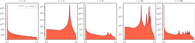
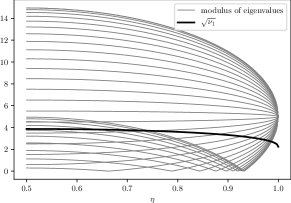
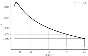
Figure 6: Top: A plot of the shape of the RHS of (45) as a function of $\eta$, for different values of $r$ ranging from $2$ to $2^{5}$, with a log-scale on the $y$-axis. The red zone represent the set of degree parameters $s$ that lie below the threshold $s(\eta,r)$ in (45): they are the values for which our method does not yield full reconstruction guarantees, since at least one eigenvalue/eigenvector couple is ‘lost in the bulk’ of the spectrum of $A$.
Bottom left: Here $s=10$ and $r=30$. The absolute values of the eigenvalues $\nu_{k}=s(1/2+c_{k}\theta)$ are plotted in grey, while the threshold $\rho=\sqrt{\nu_{1}}$ is in bold black.
Bottom right: the shape of $\eta\mapsto\eta(s)$.

E.5 Computations for the two-block case

We place ourselves in the setting of Theorem 27; recall that

$$F=\begin{bmatrix}s/2&s\eta\\ s(1-\eta)&s/2\end{bmatrix},\qquad\qquad F\Pi=\Pi F=\begin{bmatrix}s/4&s\eta/2\\ s(1-\eta)/2&s/4\end{bmatrix}\eqqcolon M.$$ (46)

Define $\theta=2\sqrt{\eta(1-\eta)}$; as in (43), the eigenvalues of $M$ are

$$\nu_{1}=\frac{s(1+\theta)}{4}\qquad\text{and}\qquad\nu_{2}=\frac{s(1-\theta)}{4},$$

with associated right and left eigenvectors

$$f_{1} =\left(\sqrt{\eta},\sqrt{1-\eta}\right) f_{2} =\left(\sqrt{\eta},-\sqrt{1-\eta}\right)$$

$$g_{1} =\left(\sqrt{1-\eta},\sqrt{\eta}\right) g_{2} =\left(\sqrt{1-\eta},-\sqrt{\eta}\right).$$

Applying Theorem 27, we have $r_{0}=2$ whenever $\nu_{2}^{2}>\nu_{1}$, which simplifies to

$$s>\frac{4(1+\theta)}{(1-\theta)^{2}},$$

which settles the first part of Theorem 8. Now, simplifying (40) whenever $i=j$, we have

$$a_{i,i}=\sqrt{\frac{\left\langle p,f^{i,i}\right\rangle}{\left\langle p,(I-\nu_{i}^{-2}M)^{-1}f^{i,i}\right\rangle}},$$

and since $p=(1/2,1/2)$ and the $f_{i}$ have unit length, this simplifies further to

$$a_{i,i}=\frac{1}{\sqrt{\left\langle\mathbf{1},(I-\nu_{i}^{-2}M)^{-1}f^{i,i}\right\rangle}}.$$ (47)

The standard adjoint formula yields, whenever $\alpha<1/\nu_{1}$,

$$(I-\alpha M)^{-1}=\frac{1}{4(1-\alpha\nu_{1})(1-\alpha\nu_{2})}\begin{pmatrix}4-\alpha s&2\alpha s\eta\\ 2\alpha s(1-\eta)&4-\alpha s,\end{pmatrix}$$

and since $f^{1,1}=f^{2,2}=(\eta,1-\eta)$, we have

$$\left\langle\mathbf{1},(I-\alpha M)^{-1}f^{i,i}\right\rangle^{-1} =\frac{4(1-\alpha\nu_{1})(1-\alpha\nu_{2})}{4-\alpha s+\alpha s\theta^{2}}$$

$$=\frac{4-2\alpha s+\alpha^{2}s^{2}\frac{1-\theta^{2}}{4}}{4-\alpha s+\alpha s\theta^{2}}$$

$$\eqqcolon\gamma(\alpha s).$$

Since we will choose $\alpha=\nu_{i}^{-2}$, we have $\alpha s->0$ and

$$\gamma(x) =\left(1-\frac{x}{2}\right)\left(1+\frac{(1-\theta^{2})x}{4}\right)+O(x^{2})$$

$$=1-\frac{1+\theta^{2}}{4}x+O(x^{2}).$$

Substituting $\alpha=\nu_{i}^{-2}$ and taking the square root, we find

$$a_{i,i}=1-\frac{1+\theta^{2}}{8}\frac{s}{\nu_{i}^{2}}+O\left(\frac{1}{s^{2}}\right)=1-\frac{2}{s}\frac{1+\theta^{2}}{(1\pm\theta)^{2}}+O\left(\frac{1}{s^{2}}\right),$$

which are the expressions in Theorem 8.

Note that it is possible to continue the computations and find explicit expressions for the $a_{i,i}$ in terms of $\eta$ and $s$, but the resulting expressions are too complex to give any more insight than the asymptotic expressions.

E.6 Computations when there are two blocks

We defined $\eta(s)$ as the unique number in $[0,1]$ such that

$$s>\frac{4(1+\theta)}{(1-\theta)^{2}}\quad\Longleftrightarrow\quad\eta>\eta(s),$$

with $\theta(\eta)=2\sqrt{\eta(1-\eta)}$ (see also Figure 6). The inverse $\theta^{-1}:[0,1]\to[1/2,1]$ is given by

$$\theta^{-1}(t)=\frac{1+\sqrt{1-t^{2}}}{2}.$$

Now, the solution $x$ of the equation

$$s=\frac{4(1+x)}{(1-x)^{2}}$$

is the solution of the quadratic $sx^{2}-(2s+4)x+s-4=0$. The discriminant is $\Delta(s)=16(2s+1)$ and the unique solution in $[0,1]$ is

$$x(s)=1+\frac{2-2\sqrt{2s+1}}{s}.$$

Finally, the smallest $\eta(s)$ for which (45) is satisfied is $\eta(s)=\theta^{-1}(x(s))$, that is,

$$\eta(s)=\frac{1+\sqrt{1-x(s)^{2}}}{2}=\frac{1+\sqrt{1-\left(1+\frac{2-2\sqrt{2s+1}}{s}\right)^{2}}}{2}.$$ (48)

It is possible to expand the term inside the square root, but with no meaningful gain. The function $\eta(s)$ has the series expansion

$$\eta(s)=\frac{1}{2}+\sqrt[4]{\frac{2}{s}}+O(s^{-3/4}),$$

but the convergence is very slow: the truncated RHS is less than one only whenever $s\geq 32$.

Appendix F Convergence of eigenvectors

The goal of this section is to prove Theorem 11. We place ourselves in the stochastic block model setting as in Section 3, with $\sigma_{g}=\sigma_{d}=\sigma$ and $q=p$. We assume that $F$ and $p$ are constant with $n$, so that the modularity matrix $M$ doesn’t depend on $n$.

F.1 Convergence of $\tilde{U}_{i}(x)$

We consider the multitype Galton-Watson trees $(\mathscr{T}_{j},o)$ as defined in Bordenave et al. [2018]: the root $o$ has type $\sigma(o)=j$, and afterwards, each vertex with type $i$ has $\mathrm{Poi}(M_{i,k})$ children of type $k$. Unlike our initial trees $T_{x}$, which are heavily $n$-dependent with node labels in $[n]$ and edge probabilities $P_{x,y}$, the tree $\mathscr{T}_{j}$ does not depend on $n$, and its labels are in $[r]$. We define on those trees the random processes

$$\mathscr{U}_{i}(j,t)=\nu_{i}^{-t}\sum_{k=1}^{r}N_{k}(\mathscr{T}_{j},t)f_{i}(k),$$

where $N_{k}(\mathscr{T}_{j},t)$ counts the number of vertices of type $k$ at depth $t$ in $\mathscr{T}_{j}$. Assume that we have chosen the $f_{i}$ such that $\phi_{i}=\Sigma_{d}f_{i}$ has unit norm; we recall that the processes $\tilde{U}_{i}(x,t)$ were defined in (27)-(28).

Lemma 31.

Let $x\in[n]$, and define $j=\sigma(x)$. Then the processes $\tilde{U}_{i}(x,t)$ and $\mathscr{U}_{i}(j,t)$ have the same distribution.

Proof.

Let $\sigma(T_{x})$ be the tree where a vertex with label $y$ is mapped to a vertex with label $\sigma(y)$. Then the root of $\sigma(T_{x})$ has label $\sigma(x)=j$. Take a vertex in $T_{x}$ with label $y$, and let $\sigma(y)=i$; the number of children of $y$ with type $k$ has distribution $\mathrm{Poi}(\tilde{M}_{yk})$, with

$$\tilde{M}_{y,k}=d_{y}\sum_{\sigma(z)=k}\frac{P_{yz}}{d_{y}}.$$

Using the definition of $P$ for the SBM, we have

$$\tilde{M}_{y,k}=\sum_{\sigma(z)=k}\frac{F_{\sigma(y),\sigma(z)}}{n}=F_{i,k}p_{k}=M_{i,k}.$$

Therefore, the laws of $\sigma(T_{x})$ and $\mathscr{T}_{j}$ coincide. Now, since there are no weights the product in (27) is equal to $1$ and we have

$$\tilde{U}_{i}(x,t)=\sum_{x_{t}}\varphi_{i}(\iota(x_{t}));$$

replacing $\varphi$ by its definition in terms of $f_{i}$,

$$\tilde{U}_{i}(x,t) =\nu_{i}^{-t}\sum_{x_{t}}f_{i}(\sigma(\iota(x_{t})))=\nu_{i}^{-t}\sum_{k=1}^{r}N_{k}(\sigma(T_{x}),t)f_{i}(k),$$

which ends the proof. ∎

This lemma allows us to translate results back and forth between the $T_{x}$ and the $\mathscr{T}_{\sigma(x)}$; we thus know from the expectation/correlation computations in Subsections C.5-C.7 that $\mathscr{U}_{i}(j,t)$ (with $j=\sigma(x)$) is a martingale with

$$\mathbf{E}[\mathscr{U}_{i}(j,t)]=f_{i}(j)\quad\text{and}\quad\mathbf{E}[\mathscr{U}_{i}(j,t)^{2}]\leqslant\Gamma_{\mathrm{right}}(i,i).$$

By the Doob martingale convergence theorem, this implies that $\mathscr{U}_{i}(j,t)$ converges in $\mathrm{L}^{2}$ as $t\to\infty$ towards a random variable $\mathscr{Z}_{i,j}$. Since we have convergence in $\mathrm{L}^{2}$, it entails

$$\mathbf{E}[\mathscr{Z}_{i,j}] =\lim_{t\to+\infty}\mathbf{E}[\mathscr{U}_{i}(j,t)]=f_{i}(j)$$

$$\mathbf{E}[\mathscr{Z}_{i,j}^{2}] =\lim_{t\to+\infty}\mathbf{E}[\mathscr{U}_{i}(j,t)^{2}]=\left[(I-\nu_{i}^{-2}M)^{-1}f^{i,i}\right](j).$$

In the last line, we used computations from Appendix D to determine the limit.

Another important fact is that the law of $\mathscr{U}_{i}(j,t)$ does not depend on $n$ whatsoever. This implies that $\mathscr{U}_{i}(j,\ell)$ converges to $\mathscr{Z}_{i,j}$ as $n\to+\infty$, which in turn yields the following proposition.

Proposition 32.

Let $Z_{i,j}$ be the limit of the random process $\mathscr{U}_{i}(j,t)$. Then,

$$\tilde{U}_{i}(x)\xrightarrow[n\to\infty]{\mathrm{L}^{2}}\mathscr{Z}_{i,\sigma(x)}.$$ (49)

F.2 Convergence of the pseudo-eigenvectors

Now that we showed convergence on the random tree, we shall use the concentration proposition 19 to translate it on the graph. Let $h:\mathbb{R}\to\mathbb{R}$ be a bounded continuous function, and define

$$f(G,x)=\frac{1}{p_{j}n}\,\mathbf{1}_{\sigma(x)=j}\,h(U_{i}(x)).$$

The function $f$ satisfies the hypotheses of Proposition 19 since $h$ is bounded, and we have

$$f(T_{x},x)=\frac{1}{p_{j}n}\,\mathbf{1}_{\sigma(x)=j}\,h(\tilde{U}_{i}(x))$$

Using Proposition 32, and the fact that $\mathrm{L}^{2}$ convergence implies convergence in distribution,

$$\mathbf{E}[\mathbf{1}_{\sigma(x)=j}\,h(\tilde{U}_{i}(x))]\to\mathbf{1}_{\sigma(x)=j}\mathbf{E}[h(\mathscr{Z}_{i,j})]$$

uniformly in $x$, so that summing over all vertices

$$\lim_{n\to+\infty}\frac{1}{p_{j}n}\sum_{\sigma(x)=j}h(U_{i}(x))=\mathbf{E}[h(\mathscr{Z}_{i,j})].$$ (50)

The above equation implies immediately that the discrete distribution of the $U_{i}(x)$ with $\sigma(x)=j$ converges weakly to $\mathscr{Z}_{i,j}$; in other words,

$$\frac{1}{p_{j}n}\sum_{\sigma(x)=j}\delta_{U_{i}(x)}\xrightarrow[n\to\infty]{\mathrm{d}}\mathscr{Z}_{i,j}.$$ (51)

F.3 Convergence of the eigenvector

Define the normalized pseudo eigenvectors:

$$\bar{U}_{i}=\frac{\sqrt{n}U_{i}}{|U_{i}|},$$

then thanks to (19) we have $|U_{i}|-\sqrt{n}\gamma\ll 1$, where

$$\gamma=\sqrt{\left\langle p,(I-\nu_{i}^{-2}M)^{-1}f^{i,i}\right\rangle}$$

from the computations in Appendix D. A consequence of our notation $\ll$ is that $\sqrt{n}/|U_{i}|$ converges in probability towards $\gamma>0$. Thanks to (51) and Slutsky’s lemma,

$$\frac{1}{p_{j}n}\sum_{\sigma(x)=j}\delta_{\bar{U}_{i}(x)}\xrightarrow[~{}n\to\infty~{}]{\mathrm{d}}Z_{i,j}\coloneqq\frac{\mathscr{Z}_{i,j}}{\gamma},$$

and consequently $Z_{i,j}$ has mean and variance

$$\mu_{i,j}=\frac{f_{i}(j)}{\sqrt{\left\langle p,(I-\nu_{i}^{-2}M)^{-1}f^{i,i}\right\rangle}}\qquad\text{and}\qquad\sigma_{i,j}^{2}=\frac{\left[(I-\nu_{i}^{-2}M)^{-1}f^{i,i}\right](j)}{\left\langle p,(I-\nu_{i}^{-2}M)^{-1}f^{i,i}\right\rangle}.$$ (52)

Now comes the last step of our proof; let $\bar{u}_{i}$ be a right eigenvector of $A$ such that $|\bar{u}_{i}|=\sqrt{n}$ (one can take $\bar{u}_{i}=\sqrt{n}u_{i}$). Then, (21) implies that

$$\left|\bar{u}_{i}-\bar{U}_{i}\right|\ll\sqrt{n}.$$ (53)

We want to show convergence for $\bar{u}_{i}$; using the Portmanteau lemma, it suffices to show bounds like (50) for Lipschitz functions. Let $h$ be a bounded function with Lipschitz constant $C$; we write

$$\left|\frac{1}{p_{j}n}\sum_{\sigma(x)=i}[h(\bar{u}_{i}(x))-h(\bar{U}_{i}(x))]\right| \leqslant\frac{1}{p_{j}n}\sum_{\sigma(x)=i}\left|h(\bar{u}_{i}(x))-h(\bar{U}_{i}(x))\right|$$

$$\leqslant\frac{C}{p_{j}n}\sum_{\sigma(x)=i}\left|\bar{u}_{i}(x)-\bar{U}_{i}(x)\right|$$

$$\leqslant\frac{C}{p_{j}n}\sqrt{p_{j}n}\left|\bar{u}_{i}-\bar{U}_{i}\right|,$$

using the Cauchy-Schwarz inequality. Using (53), we are done.

References

- Abbe [2017] Emmanuel Abbe. Community detection and stochastic block models: recent developments. The Journal of Machine Learning Research, 18(1):6446–6531, 2017.
- Abbe et al. [2020a] Emmanuel Abbe, Enric Boix-Adsera, Peter Ralli, and Colin Sandon. Graph powering and spectral robustness. SIAM Journal on Mathematics of Data Science, 2(1):132–157, 2020a.
- Abbe et al. [2020b] Emmanuel Abbe, Jianqing Fan, Kaizheng Wang, Yiqiao Zhong, et al. Entrywise eigenvector analysis of random matrices with low expected rank. Annals of Statistics, 48(3):1452–1474, 2020b.
- Benaych-Georges et al. [2019] Florent Benaych-Georges, Charles Bordenave, Antti Knowles, et al. Largest eigenvalues of sparse inhomogeneous erdős–rényi graphs. Annals of Probability, 47(3):1653–1676, 2019.
- Bordenave et al. [2018] Charles Bordenave, Marc Lelarge, and Laurent Massoulié. Nonbacktracking spectrum of random graphs: Community detection and nonregular ramanujan graphs. Ann. Probab., 46(1):1–71, 01 2018. doi: 10.1214/16-AOP1142. URL https://doi.org/10.1214/16-AOP1142.
- Bordenave et al. [2020] Charles Bordenave, Simon Coste, and Raj Rao Nadakuditi. Detection thresholds in very sparse matrix completion, 2020.
- [7] Mo Chen, Qiong Yang, Xiaoou Tang, et al. Directed graph embedding.
- Chen et al. [2018] Yuxin Chen, Chen Cheng, and Jianqing Fan. Asymmetry helps: Eigenvalue and eigenvector analyses of asymmetrically perturbed low-rank matrices. arXiv preprint arXiv:1811.12804, 2018.
- Chung [2005] Fan Chung. Laplacians and the cheeger inequality for directed graphs. Annals of Combinatorics, 9(1):1–19, 2005.
- Cucuringu et al. [2019] Mihai Cucuringu, Huan Li, He Sun, and Luca Zanetti. Hermitian matrices for clustering directed graphs: insights and applications, 2019.
- Ding et al. [2016] Zhuanlian Ding, Xingyi Zhang, Dengdi Sun, and Bin Luo. Overlapping community detection based on network decomposition. Scientific reports, 6:24115, 2016.
- Füredi and Komlós [1981] Z. Füredi and J. Komlós. The eigenvalues of random symmetric matrices. Combinatorica, 1(3):233–241, September 1981. ISSN 1439-6912. doi: 10.1007/BF02579329.
- Gao et al. [2017] Chao Gao, Zongming Ma, Anderson Y Zhang, and Harrison H Zhou. Achieving optimal misclassification proportion in stochastic block models. The Journal of Machine Learning Research, 18(1):1980–2024, 2017.
- Holland et al. [1983] Paul W Holland, Kathryn Blackmond Laskey, and Samuel Leinhardt. Stochastic blockmodels: First steps. Social networks, 5(2):109–137, 1983.
- Kannan et al. [2004] Ravi Kannan, Santosh Vempala, and Adrian Vetta. On clusterings: Good, bad and spectral. Journal of the ACM (JACM), 51(3):497–515, 2004.
- Laenen and Sun [2020] Steinar Laenen and He Sun. Higher-order spectral clustering of directed graphs, 2020.
- Leicht and Newman [2008] Elizabeth A Leicht and Mark EJ Newman. Community structure in directed networks. Physical review letters, 100(11):118703, 2008.
- Li et al. [2015] Yuemeng Li, Xintao Wu, and Aidong Lu. Analysis of spectral space properties of directed graphs using matrix perturbation theory with application in graph partition. In 2015 IEEE International Conference on Data Mining, pages 847–852. IEEE, 2015.
- Malliaros and Vazirgiannis [2013] Fragkiskos D Malliaros and Michalis Vazirgiannis. Clustering and community detection in directed networks: A survey. Physics reports, 533(4):95–142, 2013.
- Mariadassou et al. [2010] Mahendra Mariadassou, Stéphane Robin, Corinne Vacher, et al. Uncovering latent structure in valued graphs: a variational approach. The Annals of Applied Statistics, 4(2):715–742, 2010.
- Massoulié [2014] Laurent Massoulié. Community detection thresholds and the weak ramanujan property. In Proceedings of the forty-sixth annual ACM symposium on Theory of computing, pages 694–703, 2014.
- [22] Geoffrey J McLachlan and Kaye E Basford. Mixture models: Inference and applications to clustering, volume 38.
- Mossel et al. [2015] Elchanan Mossel, Joe Neeman, and Allan Sly. Reconstruction and estimation in the planted partition model. Probability Theory and Related Fields, 162(3):431–461, 2015.
- Pal and Zhu [2019] Soumik Pal and Yizhe Zhu. Community detection in the sparse hypergraph stochastic block model. arXiv preprint arXiv:1904.05981, 2019.
- Pasquini and Reichel [2006] Silvia Noschese1 Lionello Pasquini and Lothar Reichel. Tridiagonal toeplitz matrices: Properties and novel applications. 2006.
- Pedregosa et al. [2011] F. Pedregosa, G. Varoquaux, A. Gramfort, V. Michel, B. Thirion, O. Grisel, M. Blondel, P. Prettenhofer, R. Weiss, V. Dubourg, J. Vanderplas, A. Passos, D. Cournapeau, M. Brucher, M. Perrot, and E. Duchesnay. Scikit-learn: Machine learning in Python. Journal of Machine Learning Research, 12:2825–2830, 2011.
- Pentney and Meila [2005] William Pentney and Marina Meila. Spectral clustering of biological sequence data. 2005.
- Rohe et al. [2011] Karl Rohe, Sourav Chatterjee, Bin Yu, et al. Spectral clustering and the high-dimensional stochastic blockmodel. The Annals of Statistics, 39(4):1878–1915, 2011.
- Satuluri and Parthasarathy [2011] Venu Satuluri and Srinivasan Parthasarathy. Symmetrizations for clustering directed graphs. In Proceedings of the 14th International Conference on Extending Database Technology, pages 343–354, 2011.