On the Observational Difference Between the Accretion Disk-Corona Connections among Super- and Sub-Eddington Accreting Active Galactic Nuclei

Abstract

We present a systematic X-ray and multiwavelength study of a sample of 47 active galactic nuclei (AGNs) with reverberation-mapping measurements. This sample includes 21 super-Eddington accreting AGNs and 26 sub-Eddington accreting AGNs. Using high-state observations with simultaneous X-ray and UV/optical measurements, we investigate whether super-Eddington accreting AGNs exhibit different accretion disk-corona connections compared to sub-Eddington accreting AGNs. We find tight correlations between the X-ray-to-UV/optical spectral slope parameter ($\alpha_{\rm OX}$) and the monochromatic luminosity at $2500~{}{\textup{\AA}}$ ($L_{\rm 2500~{}{\textup{\AA}}}$) for both the super- and sub-Eddington subsamples. The best-fit $\alpha_{\rm OX}\textrm{--}L_{\rm 2500~{}{\textup{\AA}}}$ relations are consistent overall, indicating that super-Eddington accreting AGNs are not particularly X-ray weak in general compared to sub-Eddington accreting AGNs. We find dependences of $\alpha_{\rm OX}$ on both the Eddington ratio ($L_{\rm Bol}/L_{\rm Edd}$) and black hole mass ($M_{\rm BH}$) parameters for our full sample. A multi-variate linear regression analysis yields $\alpha_{\rm OX}=-0.13{\rm log}(L_{\rm Bol}/L_{\rm Edd})-0.10{\rm log}M_{\rm BH}-0.69$, with a scatter similar to that of the $\alpha_{\rm OX}\textrm{--}L_{\rm 2500~{}{\textup{\AA}}}$ relation. The hard (rest-frame $>2\rm~{}keV$) X-ray photon index ($\Gamma$) is strongly correlated with $L_{\rm Bol}/L_{\rm Edd}$ for the full sample and the super-Eddington subsample, but these two parameters are not significantly correlated for the sub-Eddington subsample. A fraction of super-Eddington accreting AGNs show strong X-ray variability, probably due to small-scale gas absorption, and we highlight the importance of employing high-state (intrinsic) X-ray radiation to study the accretion disk-corona connections in AGNs.

1 Introduction

Active galactic nuclei (AGNs) are powered by accretion onto central massive black holes (BHs). The inflowing gas naturally forms an accretion disk, producing luminous emission mainly in the optical and UV bands. Evidence indicates that the primary AGN X-ray emission is produced via Compton up-scattering of the accretion-disk UV/optical photons by energetic electrons in a compact corona surrounding the BH (e.g., Sunyaev & Titarchuk, 1980; Haardt & Maraschi, 1993). The emitted X-ray photon spectrum is well described with a power-law continuum with a form of $N(E)\propto E^{-\Gamma}$. The photon index ($\Gamma$) of the spectrum is expected to depend on coronal parameters such as the electron temperature and optical depth (e.g., Rybicki & Lightman, 1986; Haardt & Maraschi, 1991, 1993).

As would be expected from the paradigm described above, observations have revealed evidence that the accretion disk and X-ray corona are connected. First, there is a strong correlation between AGN UV/optical and X-ray luminosities, which is often parameterized as a relation between the optical-to-X-ray power-law slope parameter $\alpha_{\rm OX}$ and $L_{\rm 2500~{}{\textup{\AA}}}$ across a broad range in UV luminosity (e.g., Avni & Tananbaum, 1982, 1986; Kriss & Canizares, 1985; Wilkes et al., 1994; Vignali et al., 2003; Strateva et al., 2005; Steffen et al., 2006; Just et al., 2007; Gibson et al., 2008; Green et al., 2009; Lusso et al., 2010; Grupe et al., 2010; Jin et al., 2012; Laha et al., 2018; Chiaraluce et al., 2018). This correlation can also be described as the dependence of ${\sc L_{\rm 2~{}keV}}$ on $L_{2500~{}{\textup{\AA}}}$ (e.g., Tananbaum et al., 1979; Avni & Tananbaum, 1982, 1986; Wilkes et al., 1994; Strateva et al., 2005; Steffen et al., 2006; Just et al., 2007; Lusso et al., 2010; Lusso & Risaliti, 2016; Chiaraluce et al., 2018). These correlations suggest that some mechanisms (e.g., Merloni, 2003; Liu et al., 2002; Jiang et al., 2019; Arcodia et al., 2019; Cheng et al., 2020) must be in place to regulate the energetic interactions between the accretion disk and the corona. A well established $\alpha_{\rm OX}\textrm{--}L_{2500~{}{\textup{\AA}}}$ or ${\sc L_{\rm 2~{}keV}}\textrm{--}L_{2500~{}{\textup{\AA}}}$ relation can be used to identify AGNs emitting unusually weak or strong X-ray emission, relative to their UV luminosities (e.g., Gibson et al., 2008; Miller et al., 2011). A well-calibrated ${\sc L_{\rm 2~{}keV}}\textrm{--}L_{2500~{}{\textup{\AA}}}$ relation can also be used to estimate cosmological parameters (e.g., Lusso & Risaliti, 2016, 2017; Bisogni et al., 2017).

Another remarkable piece of evidence showing the disk-corona connection is the significant positive correlation between the hard X-ray photon index and Eddington ratio ($L_{\rm Bol}/L_{\rm Edd}$, where $L_{\rm Bol}$ is the bolometric luminosity and $L_{\rm Edd}$ is the Eddington luminosity; e.g., Shemmer et al. 2006, 2008; Jin et al. 2012; Risaliti et al. 2009; Brightman et al. 2013; Trakhtenbrot et al. 2017). A possible interpretation of this relationship is that in a higher $L_{\rm Bol}/L_{\rm Edd}$ system the enhanced UV/optical emission from the accretion disk results in more effective Compton cooling of the corona, decreasing its temperature and/or optical depth, which leads to the softening of the X-ray spectrum (a larger value of $\Gamma$; e.g., Haardt & Maraschi 1991, 1993; Pounds et al. 1995; Fabian et al. 2015; Cheng et al. 2020).

The AGN accretion-disk properties likely depend on the accretion rate (usually represented by $L_{\rm Bol}/L_{\rm Edd}$). Typical AGNs with $0.01\lesssim L_{\rm Bol}/L_{\rm Edd}\lesssim 0.3$ are expected to have optically thick geometrically thin accretion disks (e.g., Shakura & Sunyaev, 1973). At higher accretion rates ($L_{\rm Bol}/L_{\rm Edd}\gtrsim 0.3$), the disk likely becomes geometrically thick, as shown in the slim disk model (e.g., Abramowicz et al., 1980, 1988; Wang & Netzer, 2003; Wang et al., 2014a) and numerical simulations (e.g., Ohsuga & Mineshige, 2011; Jiang et al., 2014, 2016, 2017; Kitaki et al., 2018; Sadowski et al., 2014). The radiative efficiency of the thick disk is probably reduced compared to the thin disk, mainly due to the photon-trapping effect, although the values of the radiative efficiency predicted by numerical simulations are much larger than that of the analytic slim disk model, close to that of the thin disk. The spectral energy distribution (SED) of the thick disk is expected to be different from that of the thin disk, and the thick disk may produce enhanced extreme UV (EUV; $\sim 100\textrm{--}1200~{}\textup{\AA}$) radiation (e.g., Castelló-Mor et al., 2016; Kubota & Done, 2018). However, this difference is hard to resolve observationally due to the lack of EUV data. As a result of the changing disk structure, both the nature of the coronae and the accretion disk-corona connections may be different between super- and sub-Eddington accreting AGNs. For example, the photon-trapping effect may influence the energy transport from the accretion disk to the corona, changing the Compton cooling efficiency of hot electrons in the corona.

If super-Eddington accreting AGNs have different coronae and/or accretion disk-corona connections compared to sub-Eddington accreting AGNs, this probably manifests in altered $\alpha_{\rm OX}(L_{\rm 2~{}keV})\textrm{--}L_{\rm 2500~{}{\textup{\AA}}}$ and $\Gamma\textrm{--}L_{\rm Bol}/L_{\rm Edd}$ relations. Previous studies of these relations usually targeted samples including both super- and sub-Eddington accreting AGNs, and the two groups were not separated. There have been some suggestions that super-Eddington accreting AGNs may show relatively weak X-ray emission, deviating from the $\alpha_{\rm OX}(L_{\rm 2~{}keV})\textrm{--}L_{\rm 2500~{}{\textup{\AA}}}$ relation for sub-Eddington accreting AGNs. For example, X-ray investigations of intermediate-mass BH (IMBH) candidates with high Eddington ratios suggested that a number of IMBHs appear to have suppressed X-ray emission (e.g., Greene & Ho, 2007; Dong et al., 2012). However, weak X-ray emission observed from super-Eddington accreting AGNs might not be intrinsic, and it may instead be caused by X-ray absorption. Some narrow-line Seyfert 1 (NLS1) galaxies and quasars with high accretion rates have been found to show extreme (by factors of $>10$) X-ray variability without coordinated UV/optical variability, and they are significantly X-ray weak in the low X-ray states; their extreme X-ray weakness is probably related to the shielding of the corona by a thick inner accretion disk and its associated outflow (e.g., Liu et al., 2019; Ni et al., 2020, and references therein). In addition, although there have been some studies of the $\Gamma\textrm{--}L_{\rm Bol}/L_{\rm Edd}$ relation for AGNs with high Eddington ratios (e.g., Ai et al., 2011; Kamizasa et al., 2012), they have not compared systematically the difference between the relations among super- and sub-Eddington accreting AGNs.

In this work, we utilize an AGN sample with reverberation mapping (RM) measurements to investigate systematically the observational difference between the accretion disk-corona connections among super- and sub-Eddington accreting AGNs. The RM technique is considered to provide the most accurate measurements of BH masses for broad emission-line AGNs (e.g., Blandford & McKee, 1982; Peterson, 1993). Successful RM studies have been carried out for nearly 200 AGNs (e.g., Peterson et al., 1998, 2002, 2004; Kaspi et al., 2000, 2007; Bentz et al., 2008, 2009; Denney et al., 2009; Barth et al., 2013, 2015; Rafter et al., 2011, 2013; Du et al., 2014, 2015, 2016, 2018; Wang et al., 2014b; Shen et al., 2016; Jiang et al., 2016; Fausnaugh et al., 2017; Grier et al., 2012, 2017, 2019). Most of these campaigns do not target super-Eddington accreting AGNs. A recent campaign targeting super-Eddington accreting massive black holes (SEAMBHs) has identified about 24 candidates, which increases significantly the number of super-Eddington accreting AGNs with RM measurements (Du et al., 2014, 2015, 2016, 2018; Wang et al., 2014b). The majority of reported RM AGNs are nearby bright sources that have sensitive X-ray coverage from archival XMM-Newton (Jansen et al., 2001), Chandra (Weisskopf et al., 1996), and Swift (Gehrels et al., 2004) observations. For XMM-Newton and Swift observations, simultaneous UV/optical measurements by the same satellites are available.

The paper is organized as follows. In Section 2, we describe the sample-selection procedure, the observational data, and the methods of data reduction and analysis. In Section 3, we present the statistical analysis of the correlations between $\alpha_{\rm OX}$ ($L_{\rm 2~{}keV}$) and $L_{\rm 2500~{}{\textup{\AA}}}$, $\Gamma$ and $L_{\rm Bol}/L_{\rm Edd}$, for our super- and sub-Eddington accreting AGN subsamples. In Section 4, we discuss the implications of the correlations, and we explore the dependence of $\alpha_{\rm OX}$ on both $M_{\rm BH}$ and $L_{\rm Bol}/L_{\rm Edd}$. We summarize and present future prospects in Section 5. Throughout this paper, we use J2000 coordinates and a cosmology with $H_{0}=67.4$ km s^-1 Mpc^-1, $\Omega_{\rm M}=0.315$, and $\Omega_{\Lambda}=0.686$ (Planck Collaboration et al., 2020). All errors are quoted at a $68\%$ ($1\sigma$) confidence level.

2 Sample Properties and Data Analysis

2.1 Sample Selection

Our RM AGN sample was selected from the RM AGNs compiled by the SEAMBH collaboration (Du et al., 2015, 2016, 2018), which contains 25 targets (including 24 super-Eddington accreting AGN candidates) in the SEAMBH campaign and 50 AGNs studied in previous RM work. We selected sample objects from these 75 AGNs based on the following considerations:

(1) We selected radio-quiet AGNs, since radio-loud AGNs may have excess X-ray emission linked to the radio jets and other processes (e.g., Miller et al., 2011; Zhu et al., 2020). We searched for radio information from the literature (e.g., Kellermann et al., 1989; Wadadekar, 2004; Sikora et al., 2007) and the NASA/IPAC Extragalactic Database (NED), and we discarded five radio-loud AGNs.

(2) Since we aim to explore the intrinsic X-ray and UV/optical properties of our sample, objects affected by heavy absorption in the X-ray and UV/optical bands were excluded. We discarded 11 objects in total, nine of which are well-studied objects (PG $1700+518$, Mrk 486, NGC 4051, NGC 4151, NGC 3516, NGC 3227, NGC 3783, Mrk 5273, and MCG–6-30-15) with X-ray emission affected by ionized and/or neutral absorption related to outflows, and some of them also show continuum reddening or broad absorption lines (BALs) in their UV spectra (e.g., Pounds et al., 2004; Kraemer et al., 2005, 2006, 2012; Cappi et al., 2006; Ballo et al., 2008, 2011; Turner et al., 2011; Beuchert et al., 2015; Pahari et al., 2017; Dunn et al., 2018). A super-Eddington accreting AGN, Mrk 202, shows an unusually flat 2–10 keV spectrum and an absorption feature prominent in the $<2$ keV spectrum, so that it was also excluded. In addition, a ”changing-look” AGN, Mrk 590, has changed its optical spectral type from Type 1 to Type 1.9–2, with dramatic variation in the UV/optical and X-ray fluxes (e.g., Denney et al., 2014). It is expected to emit intrinsic X-ray and UV/optical radiation in the high state when it was classified as a Type 1 Seyfert galaxy. However, there is no X-ray observation available during the high state. We thus excluded this AGN from our study.

There are three additional AGNs that have at one time shown absorption features in the X-ray and/or UV/optical bands. A transient absorption event has been detected in Mrk 766, but its high-state X-ray spectrum does not show any absorption features (e.g., Risaliti et al., 2011; Liebmann et al., 2014). We thus retained this object and used its high-state observational data in our analysis. The 2013 XMM-Newton observation of NGC 5548 revealed that it was obscured by clumpy gas not seen before, which blocks a large fraction of its soft X-ray emission and causes UV BALs (e.g., Kaastra et al., 2014; Cappi et al., 2016). We checked its high-state X-ray and UV/optical data obtained from the 2002 XMM-Newton observation, and we found that the simultaneous X-ray and UV/optical fluxes are free from absorption. Its 2002 UV spectrum also shows no absorption features (e.g., Kaastra et al., 2014). We thus also retained this object in our study and analyzed its 2002 XMM-Newton observation. Moreover, a super-Eddington accreting AGN, IRAS F$12397+3333$, was affected by ionized absorption with flux deficiencies prominent around 0.7–1 keV, while its 2–10 keV spectrum is hardly affected by the ionized absorption (Dou et al., 2016). Its steep Balmer decrement indicates intrinsic reddening in the UV/optical (e.g., Du et al., 2014). Considering that its hard X-ray spectrum is not affected by absorption, we still included this object in our study and applied a reddening correction to its UV/optical data (see Section 2.5 and Appendix for details).

(3) The selected AGNs have good archival XMM-Newton, Chandra, or Swift coverage. Since we focused on the hard (rest-frame $>2$ keV) X-rays (see Section 2.5 below), these objects are required to be significantly detected in the rest-frame $>2$ keV band with signal-to-noise (S/N) ratios larger than 6. The XMM-Newton data have the highest priority since they have high-quality X-ray spectral data and simultaneous UV/optical data. For AGNs without XMM-Newton data, we used Chandra observations if available, otherwise, Swift observations are used. There are six AGNs without archival X-ray data, of which four are Sloan Digital Sky Survey Release 7 (SDSS-DR7) quasars in the SEAMBH campaign. In addition, there are six SDSS quasars in the SEAMBH campaign serendipitously detected by Swift with low S/N ratios. We thus discarded these 12 AGNs.

Our final sample consists of 47 RM AGNs, which are referred to as the full sample. From these objects we identified 21 super-Eddington accreting AGNs that were classified on the basis of normalized accretion rate of $\dot{\rm\mathscr{M}}\geq 3$, following the approach of the SEAMBH campaign (Wang et al., 2014b; Du et al., 2015). The normalized accretion rate is defined as $\dot{\rm\mathscr{M}}=\dot{M}c^{2}/L_{\rm Edd}$, where $\dot{M}$ is the mass accretion rate. We measured $\dot{\rm\mathscr{M}}$ based on the Shakura & Sunyaev (1973) standard thin disk model (see Section 2.6). For super-Eddington accreting AGNs, $\dot{\rm\mathscr{M}}$ may be a better indicator of the accretion rate, rather than $L_{\rm Bol}/L_{\rm Edd}$, because their bolometric luminosities may be saturated due to the photon-trapping effect (e.g., Wang et al., 2014b). The criterion of $\dot{\rm\mathscr{M}}\geq 3$ corresponds to $L_{\rm Bol}/L_{\rm Edd}\geq 0.3$ for a typical radiative efficiency of $\eta=0.1$. We refer to the 21 super-Eddington accreting AGNs as the super-Eddington subsample. The remaining 26 objects constitute the sub-Eddington subsample.

Table 1 lists the basic properties of our sample AGNs including $5100~{}\textup{\AA}$ luminosities, H$\beta$ FWHMs, and BH masses ($M_{\rm BH}$) and associated measurement uncertainties, which were adopted from Du et al. (2015, 2016); Du & Wang (2019). We note that there may be considerable systematic uncertainties on the RM BH masses (see Section 4.3 below for discussion), which are difficult to quantify. We thus only take into account the measurement uncertainties in the following analyses. For the full sample, the measurement uncertainties on $M_{\rm BH}$ range from 0.03 to 0.40 dex, with a median value of 0.13 dex. Figure 1 shows the distribution of our sample AGNs in the redshift versus $2500~{}{\textup{\AA}}$ luminosity plane. For all sample objects (except SDSS J$085946+274534$), the $2500~{}{\textup{\AA}}$ luminosities were derived from the UV/optical data that were observed simultaneously with the X-ray data (see detailed analyses in the following subsections). The distributions of the $2500~{}{\textup{\AA}}$ luminosities for the super- and sub-Eddington subsamples are comparable.

Some of our sample objects are well-studied AGNs with multiple X-ray observations. For these objects, we used their high-state observational data, which likely correspond to the intrinsic X-ray emission. There are three super-Eddington subsample objects (Mrk 335, PG $1211+143$, and PG $0844+349$) displaying extreme X-ray variability by factors of larger than 10 (e.g., Gallagher et al., 2001; Grupe et al., 2007; Bachev et al., 2009; Gallo et al., 2011; Grupe et al., 2012; Gallo et al., 2018). Their high-state X-ray observations reveal X-ray fluxes consistent with the levels expected from their UV/optical emission, likely reflecting their intrinsic X-ray properties (see notes on individual sources in Appendix). Moreover, we included two ”changing-look” AGNs with sub-Eddington accretion rates (NGC 2617: Shappee et al. 2014; Giustini et al. 2017; Mrk 1310: Luo B. et al. in preparation; see details in Appendix). They have undergone changes in their optical spectral types and UV/optical and X-ray fluxes. We used their observational data in the historical high states, when they exhibit strong broad optical emission lines and the brightest X-ray and UV/optical luminosities. A list of the X-ray observations used in this study is presented in Table 2.

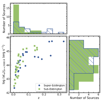
Figure 1: Redshift vs. $2500~{}{\textup{\AA}}$ luminosity for the super-Eddington subsample (blue circles) and the sub-Eddington subsample (green squares). The right panel shows the distribution of $2500~{}{\textup{\AA}}$ luminosity, and the upper panel shows the distribution of redshift. The super-Eddington (sub-Eddington) subsample is represented by the hatched blue (filled green) histograms.

2.2 XMM-Newton Observations

XMM-Newton data are available for 37 sample AGNs. Except for one AGN, SBS 1116+583A, all these AGNs were targets of the corresponding XMM-Newton observations. Simultaneous X-ray and UV/optical data were obtained from the European Photon Imaging Camera (EPIC) PN (Strüder et al., 2001) and MOS (Turner et al., 2001) detectors, and the Optical Monitor (OM; Mason et al., 2001). We processed the data using the XMM-Newton Science Analysis System (SAS v.16.0.0), and the latest calibration files were applied. For the X-ray analysis, we only used the EPIC PN data. The task epproc was first used to reduce the PN data and create the calibrated event lists. Bad or hot pixels were removed from the event lists, and high-background flares were checked and filtered according to the standard criteria. Only single and double events (PATTERN$\leq 4$ and FLAG=0) were selected. A circular region with a default radius of 35″ was used to extract the source spectrum. Each data set was inspected for pile-up by running the task epatplot. For nine sources with detected pile-up (see Table 2), an inner circular region with a radius of 5–10″ was discarded from the source extraction region. These are bright X-ray sources, and the extracted spectra still have high quality, allowing robust spectral fitting. The background spectrum was extracted from a nearby source-free circular region with a radius of 50–100″ on the same CCD chip. The response matrix and ancillary response function files were created using the tasks rmfgen and arfgen, which account for the point spread function correction of the source-extraction region. The final PN spectrum was grouped with a minimum number of one count per bin using the task specgroup.

We analyzed OM data mainly for deriving flux densities at the rest-frame $2500~{}{\textup{\AA}}$ band. OM imaging data are available for all sample objects, except for Mrk 335 with only UV grism data in its selected observation. There are six OM filters, including three optical filters (V, B, U with central wavelengths of 5430 Å, 4500 Å, 3440 Å) and three UV filters (UVW1, UVM2, UVW2 with central wavelengths of 2910 Å, 2320 Å, 2110 Å). We processed the OM filter data using the pipeline omchian. Point sources and extended sources were automatically identified as part of the pipeline. Source fluxes and magnitudes were extracted from the SWSRLI files, and we adopted the mean magnitudes and fluxes of all the exposure segments for each filter. For Mrk 335, the OM UV grism data were processed with the pipeline omghian. The pipeline generated 24 calibrated spectra, and the spectra cover a wavelength range of $1800\textrm{--}3600~{}{\textup{\AA}}$. The fluxes of the OM filters and the mean grism spectra were then corrected for Galactic extinction using the extinction law of Cardelli et al. (1989). Table 1 lists the mean values of Galactic extinction $E_{\rm B-V}$ (Schlegel et al., 1998) that were obtained from the NASA/IPAC Infrared (IR) Science Archive.

We utilized the OM UV-filter flux densities to derive the $2500~{}{\textup{\AA}}$ flux densities. Our sample objects are bright, and at least in the UV-filter images, they were identified as point sources. Therefore, host-galaxy contamination in the UV-filter fluxes should be mild (see Grupe et al. 2010 for discussion regarding the Swift UV/optical photometric data), and we did not correct the source fluxes and magnitudes for any host-galaxy contamination. Eleven out of the 36 objects with OM imaging data were observed with three UV filters, and another 14 objects were observed with two filters. We derived their $2500~{}{\textup{\AA}}$ flux densities by fitting a power-law model to the observed data. For eight objects observed with only one UV filter, the $2500~{}{\textup{\AA}}$ flux densities were extrapolated assuming a power-law slope of $\alpha_{\nu}=-0.44$ (e.g., Vanden Berk et al., 2001). For three other objects without UV-filter data, NGC 5548, NGC 6814 and PG $0844+349$, their $2500~{}{\textup{\AA}}$ flux densities were extrapolated from the U-filter flux densities assuming the same power-law slope of $\alpha_{\nu}=-0.44$. Finally, the $2500~{}{\textup{\AA}}$ flux density of Mrk 335 was measured from the mean grism spectrum. The UV-filter information and the derived $L_{2500~{}\textup{\AA}}$ values are listed in Table 2.

2.3 Chandra Observations

We used Chandra data for only one object, SDSS J$085946+274534$. It was observed as a target on 2004 December 25. The observational data were analyzed using the Chandra Interactive Analysis of Observations (CIAO; v4.11) tools. A new level 2 event file was generated using the chandra_repro script, and high-background flares were filtered by running the deflare script with an iterative 3$\sigma$ clipping algorithm. A 0.5–7 keV image was then constructed by running the dmcopy script. The specextract tool was used to extract and group spectra (with at least one count per bin), and to generate the response matrix and ancillary response function files. The source-extraction region is a circular region with a radius of 3″, centered on the X-ray source position detected by the automated source-detection tool wavdetect. An annulus region centered on the X-ray source position with a 10″ inner radius and a 30″ outer radius was chosen as the background-extraction region. The extracted source spectrum was grouped with a minimum number of one count per bin.

There are no simultaneous UV/optical data available for this Chandra object. We interpolated its Near-UV (NUV) flux density, observed on 2006 February 18, from Galaxy Evolution Explorer (GALEX; Martin et al., 2005) and SDSS u-band flux density, observed on 2004 April 17, to derive the $2500~{}{\textup{\AA}}$ flux density.

2.4 Swift Observations

We used Swift data for nine AGNs. Simultaneous X-ray and UV/optical data are available from the X-ray Telescope (XRT; Burrows et al. 2005) and the UV-Optical Telescope (UVOT; Roming et al. 2005). For all observations, the XRT was operated in the Photon Counting (PC) mode (Hill et al., 2004). The data were reduced with the task xrtpipeline version 0.13.4, which is included in the HEASOFT package 6.25. The XRT data were not affected by photon pipe-up given the low count rates ($0.02\textrm{--}0.14\ \rm counts\ s^{-1}$) of these nine AGNs. For each source, the source photons were extracted using the task xselect version 2.4, from a circular region with a radius of 47″. The background spectrum was extracted from a nearby source-free circular region with a radius of 100″. The ancillary response function file was generated by xrtmkarf, and the standard photon redistribution matrix file was obtained from the CALDB. We grouped the spectra using grppha such that each bin contains at least one photon.

The UVOT has a similar set of filters (V, B, U, UVW1, UVM2, UVW2 with central wavelengths of 5468 Å, 4392 Å, 3465 Å, 2600 Å, 2246 Å, and 1928 Å) to the OM. Similarly, we used mainly the UV-filter data to derive the $2500~{}{\textup{\AA}}$ flux densities. Among these nine Swift AGNs, six were observed with one UV filter, one was observed with two UV filters, and two were observed with three UV filters. The data from each segment in each filter were co-added using the task uvotimsum after aspect correction. Source counts were selected from a circular region with a radius of 5″, centered on the source position determined by the task uvotdetect Freeman et al. (2002). A nearby source-free region with a radius of 20″ was used to extract background counts. Source magnitudes and fluxes in each UVOT filter were then computed using the task uvotsource, and these data were corrected for Galactic extinction. We derived the $2500~{}{\textup{\AA}}$ flux densities following the same procedure as used for the OM photometric data.

2.5 X-ray Spectral Analysis

X-ray spectral analysis was performed with XSPEC (v12.10.1; Arnaud 1996). All spectra were grouped with at least one count per bin, and the Cash statistic (CSTAT; Cash 1979) was applied in parameter estimation; the W statistic was actually used because the background spectrum was included in the spectral fitting. Since the aim of this study is to obtain properties of the intrinsic coronal X-ray radiation, we focused only on the rest-frame $>2~{}\rm keV$ energy band, where the observed X-ray emission is less affected by contamination from a potential soft excess component and intrinsic absorption (e.g., Shemmer et al., 2006, 2008; Risaliti et al., 2009; Brightman et al., 2013). The rest-frame $<2~{}\rm keV$ spectral data were also analyzed with basic phenomenological models, in order to construct broad-band SEDs and provide more reliable estimates of bolometric luminosities for our sample objects (see Section 2.7 below).

We adopted a power-law model modified by Galactic absorption (phabs*zpowerlw) to fit the rest-frame $>2~{}\rm keV$ spectra, corresponding to the observed-frame $2/(1+z)\textrm{--}10~{}\rm keV$ spectra for XMM-Newton and Swift observations and the observed-frame $2/(1+z)\textrm{--}7~{}\rm keV$ spectra for the Chandra observation. We visually inspected whether there are strong iron K lines in the spectra. For 25 AGNs in which the iron K lines were detected, the rest-frame $5.5\textrm{--}7.5~{}\rm keV$ spectra were discarded in the spectral fitting. The Galactic neutral hydrogen column density toward each source was fixed at the value from Dickey & Lockman (1990). For all objects, the statistics of the best-fit models are acceptable (see Table 2), and the fitting residuals are distributed close to zero without any apparent systematic excesses/deficiencies. As shown in Figure 2, the photon indices ($\Gamma$) of the full sample span a range of $1.50\textrm{--}2.46$ with a median value of 1.94. In general, the super-Eddington subsample has larger (softer) photon indices than the sub-Eddington subsample.

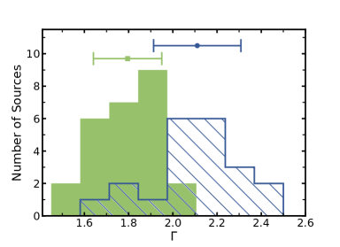
Figure 2: Distribution of the X-ray spectral photon indices for the super-Eddington (hatched blue histograms) and sub-Eddington (filled green histograms) subsamples. The two points with error bars on the top show the mean values and $1\sigma$ deviations for the two subsamples. The two subsamples are clearly distinct, with super-Eddington accreting AGNs showing steeper (softer) hard X-ray spectra.

Since we have discarded X-ray and UV/optical absorbed AGNs from our sample, and the high-state data for objects with multiple observations were used, it is likely that intrinsic absorption has little impact on the derived X-ray properties of our sample. To confirm this, we checked for the presence of intrinsic absorption in each object by adding an intrinsic neutral absorption component (zphabs model in XSPEC) to the fitting model. For each object, the best-fit statistic did not change significantly, and the resulting column density is consistent with zero; an F test also indicated that the absorption component is likely not required. Moreover, we extrapolated the data-to-model ratios of the best-fit simple power-law model (not including the intrinsic absorption component) to the entire spectral energy range (0.3–10 keV for XMM-Newton and Swift observations and 0.5–7 keV for the Chandra observation) to inspect whether absorption is present at rest-frame $<2~{}\rm keV$ energies. Only IRAS F$12397+3333$ shows flux deficiencies in the $\approx$ 0.7–1 keV band. It was reported by Dou et al. (2016) that the 0.3–10 keV spectral fitting with a model including ionized absorption and soft excess components yields an intrinsic photon index of 2.2, which is consistent with the photon index obtained by fitting the 2–10 keV spectrum with a simple power-law model. Our simple power-law fitting of the rest-frame $>2~{}\rm keV$ spectrum also resulted in a consistent photon index of 2.14. We thus conclude that the rest-frame $>2~{}\rm keV$ spectrum of IRAS F$12397+3333$ is intrinsic. Therefore, for all objects, we adopted the results from the spectral fitting performed with the simple power-law model modified with Galactic absorption. The flux densities at rest-frame 2 keV ($f_{\rm 2~{}keV}$) were then computed based on the best-fit models. The best-fit model parameters and fitting statistics are presented in Table 2.

2.6 Estimation of Normalized Accretion Rates

The Shakura & Sunyaev (1973) standard thin disk model predicts a power-law SED in the form of $F_{\nu}\propto\nu^{1/3}$ from optical to NUV, and the monochromatic luminosity at a given wavelength depends on the BH mass and accretion rate (e.g., Equation 5 of Davis & Laor 2011). Given the observed SED and the BH mass, the accretion rate ($\dot{M}$ or $\dot{\rm\mathscr{M}}$) can be computed (e.g., Davis & Laor, 2011; Netzer, 2013; Wang et al., 2014b). We used the monochromatic luminosity at $2500~{}\textup{\AA}$ to calculate $\dot{\rm\mathscr{M}}$ following the expression:

$$\dot{\rm\mathscr{M}}=4.82(\ell_{44}/{\cos i})^{3/2}m_{7}^{-2},$$ (1)

where $\ell_{44}=\nu L_{2500~{}\textup{\AA}}/10^{44}~{}\rm erg~{}s^{-1}$ is the $2500~{}\textup{\AA}$ luminosity in units of $10^{44}~{}\rm erg~{}s^{-1}$, $m_{7}=M_{\rm BH}/10^{7}M_{\odot}$, and i is the inclination angle of the disk. For Type 1 AGNs, the dependence of $\dot{\rm\mathscr{M}}$ on cos i is weak, and thus we adopted a median cos i value of 0.75. We adopted the $2500~{}\textup{\AA}$ luminosity instead of the $5100~{}\textup{\AA}$ luminosity that is often used to calculate $\dot{\rm\mathscr{M}}$ in previous studies, because the emission around $2500~{}\textup{\AA}$ is less affected by host-galaxy contamination that is significant for nearby moderate-luminosity AGNs. Moreover, for most sample objects, the $2500~{}\textup{\AA}$ luminosities were derived from the UV/optical data that were observed simultaneously with the X-ray data, and thus the accretion-disk corona connections explored below are free from any variability effects. For the full sample, the $\dot{\rm\mathscr{M}}$ values span a range of $0.012$ to $530$, with a median value of $0.83$. The uncertainties on $\dot{\rm\mathscr{M}}$ are propagated from the measurement uncertainties on $M_{\rm BH}$ and the $2500~{}\textup{\AA}$ luminosities. Table 1 lists the ${\rm log}\dot{\rm\mathscr{M}}$ values and their uncertainties.

We note that Equation 1 likely also holds for super-Eddington accreting AGNs (e.g., Du et al., 2016; Huang et al., 2020), where the accretion disks are expected to be geometrically thick. Based on the self-similar solution of the slim disk model (Wang & Zhou, 1999; Wang et al., 1999), the radius of the disk region emitting $2500~{}\textup{\AA}$ photons is larger than the photon-trapping radius for our sample objects. Observationally, studies of the SEDs of super-Eddington accreting AGNs revealed that their UV/optical SEDs are well-fitted by the thin disk model, and the characteristics of the thick-disk emission likely emerge in the EUV (e.g., Castelló-Mor et al. 2016; Kubota & Done 2018). It is also supported by our finding that the high-luminosity super-Eddington accreting AGNs in our sample show UV/optical SEDs consistent with those of typical quasars (see Section 3.4). Furthermore, a recent accretion-disk reverberation mapping on a super-Eddington accreting AGN, Mrk 142, found that the UV/optical (rest-frame $\approx 1845\textrm{--}8325\ \textup{\AA}$) wavelength-dependent lags generally follow $\tau(\lambda)\propto\lambda^{4/3}$, as expected from a thin disk (Cackett et al., 2020); this result also supports the idea that the emission at $2500~{}\textup{\AA}$ likely comes from a thin disk.

2.7 Bolometric Luminosities and Eddington Ratios

Considering that most objects in our sample are nearby moderate-luminosity AGNs, for which the IR-to-UV SEDs may have significant contamination from the host galaxies, we used an IR-to-UV quasar SED template scaled to the $2500~{}\textup{\AA}$ luminosity plus the observed X-ray SED to estimate the bolometric luminosity for each object. An example of such an IR-to-X-ray SED (for PG $0844+349$) is shown in Figure 3. We adopted the luminosity-dependent mean quasar SED (low luminosity: ${\rm log}(\nu L_{\nu})|_{\lambda=2500~{}\textup{\AA}}\leq 45.41$; mid luminosity: $45.41\leq{\rm log}(\nu L_{\nu})|_{\lambda=2500~{}\textup{\AA}}\leq 45.85$) in Krawczyk et al. (2013) as the IR-to-UV template, and it was normalized to the $2500~{}\textup{\AA}$ luminosity that was derived from the UV/optical photometric data (Sections 2.2–2.4). As shown in Section 3.4 below, this mean quasar SED also describes reasonably well the optical-to-UV SEDs of super-Eddington accreting AGNs. Most of the AGN IR ($\sim 1\textrm{--}30~{}\rm\mu m$) radiation is likely reprocessed emission from the “dusty torus”, which should not be included in the computation of the bolometric luminosity (e.g., Krawczyk et al., 2013, and references therein). We thus replaced the $1\textrm{--}30~{}\rm\mu m$ SED template with an $\alpha_{\nu}=1/3$ power law (Shakura & Sunyaev, 1973) to account for the IR emission from the accretion disk (see discussion in Section 3.1 of Davis & Laor, 2011).

In the X-ray band, the rest-frame 2–10 keV SED was obtained from the rest-frame $>2~{}\rm keV$ spectral fitting result (see Section 2.5). Soft excess emission is visible for most of our sample objects when extrapolating the hard X-ray power-law models to rest-frame $<2~{}\rm keV$ energies. In order to describe better the shape of the soft X-ray SEDs, and thus measure the rest-frame $0.3\textrm{--}2$ keV X-ray luminosities, we applied simple models to fit the soft X-ray spectra (observed-frame data from 0.3 keV to $2/(1+z)$ keV for XMM-Newton and Swift observations and 0.5 keV to $2/(1+z)$ keV for the Chandra observation). The procedure is described as follows: (1) We first attempted to fit the soft X-ray spectra with a power-law model modified by Galactic absorption. This model fits well the spectra for 24 objects. (2) For the other 23 objects, their soft X-ray spectra are not described well by the power-law model with substantial residuals shown in the data vs. model plots. Therefore, we fitted the soft X-ray spectra with a thermal-Comptonization component (comptt in XSPEC) plus a power-law model, where the power-law component accounts for the coronal emission and was fixed to that constrained from the rest-frame $>2~{}\rm keV$ spectral fitting (Section 2.5). For five of the 23 objects (e.g., IRAS F$12397+3333$), we also added an additional partial-covering ionized absorption component (zxipcf) into the fitting to account for weak absorption in the soft X-rays; such absorption does not affect significantly the rest-frame $>2$ keV spectra. Table 3 lists for each of our sample objects the best-fit parameters in the soft X-rays. We note that the fitting method described above provides phenomenological descriptions of the soft X-ray continua for luminosity estimates. The best-fit models do not account for the broad-band X-ray spectra, and thus the best-fit parameters (e.g., absorption column density, temperature of the warm-corona electrons) are not necessarily physical. The final rest-frame 0.3–2 keV SEDs were derived from the best-fit models that were corrected for Galactic absorption, and the rest-frame 0.3–2 keV luminosities are listed in Table 3. We set the $912~{}\textup{\AA}\textrm{--}0.3$ keV SED to a power law connecting the two endpoints of the IR-to-UV SED template and the X-ray SED (e.g., Section 4.1 of Laor et al., 1997).

Through integrating the constructed IR-to-X-ray ($30~{}\mu\rm m\textrm{--}10~{}\rm keV$) SEDs, we obtained the bolometric luminosities for our sample, which span a range of $1.1\times 10^{43}$ to $\rm 2.3\times 10^{46}~{}erg~{}s^{-1}$. We used the uncertainties on $L_{\rm 2500~{}\textup{\AA}}$ and the 0.2–10 keV X-ray luminosities to compute the measurement uncertainties on $L_{\rm Bol}$. Given the $L_{\rm Bol}$ and $M_{\rm BH}$ values, we derived $L_{\rm Bol}/L_{\rm Edd}$ for our sample, which range from $6.7\times 10^{-3}$ to $5.5$, with a median value of $0.14$. The uncertainties on $L_{\rm Bol}/L_{\rm Edd}$ are propagated from the measurement uncertainties on $L_{\rm Bol}$ and $M_{\rm BH}$. The uncertainty on $L_{\rm Bol}/L_{\rm Edd}$ is dominated by the $M_{\rm BH}$ uncertainty, and the contribution from the $L_{\rm Bol}$ uncertainty is negligible. We note that there are potential systematic uncertainties on both $M_{\rm BH}$ and $L_{\rm Bol}$ that may introduce additional uncertainties for the $L_{\rm Bol}/L_{\rm Edd}$ estimates (see discussion in Section 4.3 below). Table 1 lists the ${\rm log}(L_{\rm Bol}$) and ${\rm log}(L_{\rm Bol}/L_{\rm Edd}$) values and associated uncertainties.

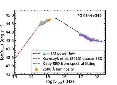
Figure 3: An example of the SED used to estimate the bolometric luminosity. The gray dots show the observed UV/optical photometric data points (see Section 3.4 for details). The purple symbols represent the X-ray spectral data points that have been corrected for the Galactic absorption; the 5.5–7.5 keV spectrum was discarded due to strong iron K emission. The IR-to-UV SED template is normalized to the $2500~{}\textup{\AA}$ luminosity that is extrapolated from the UV photometric data. The $912~{}\textup{\AA}\textrm{--}0.3$ keV SED (shown as the black dashed line) is a power law connecting the IR-to-UV SED template and the X-ray SED derived from spectral fitting (a $0.3\textrm{--}2$ keV zpowerlw model plus a $2\textrm{--}10$ keV zpowerlw model; see Tables 2 and 3).

3 Results

3.1 $\alpha_{\rm OX}$ versus $L_{2500~{}{\textup{\AA}}}$ Correlation

Figure 4 displays $\alpha_{\rm OX}$ versus ${\rm log}(L_{2500~{}{\textup{\AA}}})$ for our super-Eddington and sub-Eddington subsamples. The two parameters are highly correlated for both subsamples. For the super-Eddington (sub-Eddington) subsample, the Spearman rank correlation test gives a correlation coefficient of $r_{s}=-0.84$ ($r_{s}=-0.77$) and a $p$-value of $p=2.97\times 10^{-6}$ ($p=2.67\times 10^{-6}$). The $p$-value indicates the probability of obtaining a correlation coefficient $r_{s}$ at least as high as the observed one, under the null hypothesis that the two sets of data are uncorrelated.

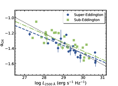
Figure 4: X-ray-to-optical power-law slope ($\alpha_{\rm OX}$) vs. $2500~{}{\textup{\AA}}$ luminosity for the super-Eddington subsample (blue circles) and the sub-Eddington subsample (green squares). The blue dashed (green dot-dashed) line shows the best-fit relation for the super-Eddington (sub-Eddington) subsample, given by Equation 2 (Equation 3). For comparison, the best-fit relation of Steffen et al. (2006) is denoted with the black dotted line.

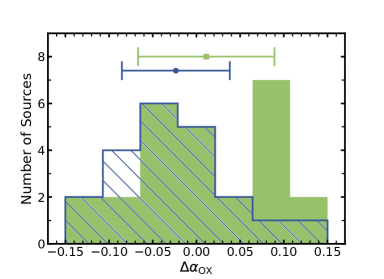
Figure 5: Distribution of $\Delta\alpha_{\rm OX}$ for the super-Eddington (hatched blue histograms) and sub-Eddington (filled green histograms) subsamples. $\Delta\alpha_{\rm OX}$ is defined as the difference between the observed $\alpha_{\rm OX}$ value and the one expected from the Steffen et al. (2006) relation (shown as the black dotted line in Figure 4). The two points with error bars on the top show the mean values and $1\sigma$ deviations for the two subsamples. The two subsamples are consistent in the $\Delta\alpha_{\rm OX}$ distribution.

We performed linear regression analysis on the $\alpha_{\rm OX}$ versus ${\rm log}(L_{2500~{}{\textup{\AA}}})$ relations, using the LINMIX_ERR method (Kelly, 2007). This is a Bayesian method that accounts for measurement uncertainties. For the super-Eddington subsample, the best-fit regression equation with the $1\sigma$ uncertainty on each parameter is

$$\alpha_{\rm OX}=(-0.11\pm 0.02){\rm log}(L_{2500~{}{\textup{\AA}}})+(1.7\pm 0.6),$$ (2)

with a scatter of 0.06. For the sub-Eddington subsample, the best-fit relation is

$$\alpha_{\rm OX}=(-0.11\pm 0.02){\rm log}(L_{2500~{}{\textup{\AA}}})+(1.9\pm 0.5),$$ (3)

with a scatter of 0.08. The relations (slopes and intercepts) for the two subsamples are consistent within their $1~{}\sigma$ uncertainties.

We then performed linear regression on the full sample, and the best-fit relation is

$$\alpha_{\rm OX}=(-0.11\pm 0.01){\rm log}(L_{2500~{}{\textup{\AA}}})+(1.9\pm 0.4),$$ (4)

with a scatter of 0.07. The relation slope is consistent within the $1\sigma$ uncertainties with those for the super-Eddington and sub-Eddington subsamples. Compared to previous results, our slope for the full sample is flatter than the slopes of $-0.14$ to $-0.22$ reported in most of the previous studies (Strateva et al., 2005; Steffen et al., 2006; Just et al., 2007; Gibson et al., 2008; Lusso et al., 2010; Chiaraluce et al., 2018; Timlin et al., 2020), but it is steeper than the slopes of $-0.06$ to $-0.07$ found by Green et al. (2009); Jin et al. (2012). Steffen et al. (2006) have suggested that the power-law slope of the $\alpha_{\rm OX}\textrm{--}L_{2500~{}{\textup{\AA}}}$ relation may be $L_{2500~{}{\textup{\AA}}}$ dependent, and it appears to be steeper towards higher $L_{2500~{}{\textup{\AA}}}$. Studies of this relation for high-luminosity quasars did find steeper slopes (e.g., Gibson et al., 2008; Timlin et al., 2020). Therefore, the flat slope for our sample may be due to the generally lower UV luminosities. The best-fit relations for the two subsamples are plotted in Figure 4. For comparison, we also plotted in Figure 4 the relation of Steffen et al. (2006) with a dotted line.

We further investigated the distribution of the $\Delta\alpha_{\rm OX}$ parameter, defined as the difference between the observed $\alpha_{\rm OX}$ value and the one expected from the $\alpha_{\rm OX}\textrm{--}L_{2500~{}{\textup{\AA}}}$ relation for typical AGNs. Considering that our full sample may be biased toward super-Eddington accreting AGNs, we adopted the Steffen et al. (2006) $\alpha_{\rm OX}\textrm{--}L_{2500~{}{\textup{\AA}}}$ relation, $\alpha_{\rm OX}=-0.137\times{\rm log}(L_{2500~{}{\textup{\AA}}})+2.638$, which was derived from a large sample of 333 typical AGNs, to compute the expected $\alpha_{\rm OX}$ values. The parameter $\Delta\alpha_{\rm OX}$ is an indicator of the level of X-ray weakness. As shown in Figure 5, the $\Delta\alpha_{\rm OX}$ distributions for the two subsamples span the same range of $-0.15$ to 0.15, which is within the rms scatter of the Steffen et al. (2006) $\alpha_{\rm OX}\textrm{--}L_{2500~{}{\textup{\AA}}}$relation. The mean and rms of the $\Delta\alpha_{\rm OX}$ values for the super-Eddington (sub-Eddington) subsample are $-0.024$ ($0.011$) and $0.062$ ($0.078$), respectively. Therefore, the super-Eddington subsample shows slightly weaker ($\approx 23\%$ lower) X-ray emission compared to the sub-Eddington subsample, but the significance of the difference is only $0.3\sigma$. A Kolmogorov-Smirnov (KS) test on the $\Delta\alpha_{\rm OX}$ distributions for the two subsamples yielded $d=0.328$ and $p=0.131$, indicating that the two distributions are similar. We note that these results would not change significantly if we instead use the best-fit $\alpha_{\rm OX}\textrm{--}L_{2500~{}{\textup{\AA}}}$ relation (Equation 4) for our full sample to compute the expected $\alpha_{\rm OX}$ values. These results suggest that both the super- and sub-Eddington subsamples show generally normal X-ray emission, when the high-state data are considered.

3.2 $L_{\rm 2~{}keV}$ versus $L_{2500~{}{\textup{\AA}}}$ Correlation

We also investigated the correlations between $L_{\rm 2~{}keV}$ and $L_{2500~{}{\textup{\AA}}}$ for our sample, shown in Figure 6. The correlations for both the super- and sub-Eddington subsamples are highly significant with Spearman coefficients of $r_{s}=0.91$ and $r_{s}=0.93$, respectively. We performed regression analysis with the LINMIX_ERR method on the two sets of parameters. For the super-Eddington subsample, the best-fit relation is

$${\rm log}(L_{\rm 2~{}keV})=(0.73\pm 0.05){\rm log}(L_{2500~{}{\textup{\AA}}})+(4.3\pm 1.4),$$ (5)

with a scatter of 0.17. For the sub-Eddington subsample, the best-fit relation is

$${\rm log}(L_{\rm 2~{}keV})=(0.71\pm 0.05){\rm log}(L_{2500~{}{\textup{\AA}}})+(5.0\pm 1.5),$$ (6)

with a scatter of 0.22. The slopes and intercepts of the relations for the two subsamples are consistent within the $1\sigma$ uncertainties. The best-fit relation for the full sample is

$${\rm log}(L_{\rm 2~{}keV})=(0.71\pm 0.03){\rm log}(L_{2500~{}{\textup{\AA}}})+(5.0\pm 1.0)\ ,$$ (7)

with a scatter of 0.19. The slope of the relation for the full sample is consistent with those ($\approx$ 0.7–0.8) reported in previous studies (e.g., Vignali et al., 2003; Strateva et al., 2005; Steffen et al., 2006; Just et al., 2007; Lusso et al., 2010; Lusso & Risaliti, 2016). We note that Equations 5, 6 and 7 can be derived from Equations 2, 3 and 4, respectively, since $\alpha_{\rm OX}$ is defined as the ratio between $L_{\rm 2~{}keV}$ and $L_{2500~{}{\textup{\AA}}}$.

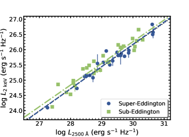
Figure 6: Rest-frame 2 keV monochromatic luminosity vs. rest-frame $2500~{}{\textup{\AA}}$ monochromatic luminosity for the super-Eddington subsample (blue circles) and the sub-Eddington subsample (green squares). The blue dashed (green dot-dashed) line shows the best-fit relation for the super-Eddington (sub-Eddington) subsample, given by Equation 5 (Equation 6). For comparison, the best-fit relation of Steffen et al. (2006) is shown with the black doted line, which follows very closely with the blue-dashed line that denotes the relation for the super-Eddington subsample.

3.3 Correlation between $\Gamma$ and accretion rate

Figure 7 plots $\Gamma$ versus ${\rm log}(L_{\rm Bol}/L_{\rm Edd})$ for our sample objects. For the full sample, a highly significant correlation is present, and the Spearman rank correlation test resulted in a correlation coefficient of $r_{s}=0.72$ with a $p$-value of $p=1.27\times 10^{-8}$. The correlation is significant for the super-Eddington subsample ($r_{s}=0.60$ and $p=0.004$); however, there is no statistically significant correlation between $\Gamma$ and ${\rm log}(L_{\rm Bol}/L_{\rm Edd})$ for the sub-Eddington subsample ($r_{s}=0.21$ and $p=0.30$). We then performed linear regression analysis on the super-Eddington subsample and the full sample with the LINMIX_ERR method, considering the measurement uncertainties on both $\Gamma$ and $L_{\rm Bol}/L_{\rm Edd}$ in the fitting. The best-fit relation for the super-Eddington subsample is

$$\Gamma=(0.33\pm 0.13){\rm log}(L_{\rm Bol}/L_{\rm Edd})+(2.15\pm 0.04),$$ (8)

with a scatter of 0.14. For the full sample, we obtained a best-fit relation:

$$\Gamma=(0.27\pm 0.04){\rm log}(L_{\rm Bol}/L_{\rm Edd})+(2.14\pm 0.04)\ ,$$ (9)

with a scatter of 0.14. Our relation slope for the full sample is consistent with the slope ($0.31\pm 0.01$) reported in Shemmer et al. (2008) for their high-redshift quasars with BH masses determined based on the $\rm H\beta$ emission lines using the single-epoch virial mass method. A similar slope ($0.32\pm 0.05$) was found by Brightman et al. (2013) for their sample with BH masses obtained from either $\rm H\beta$ or Mg II-based single-epoch estimators. However, Risaliti et al. (2009) reported a steeper slope ($0.58\pm 0.11$) for their subsample with $\rm H\beta$-based single-epoch BH masses. A steep slope ($\approx 0.57$) was also found by Jin et al. (2012), for their AGN sample with $\Gamma$ and $L_{\rm Bol}/L_{\rm Edd}$ estimated from the UV/optical-to-X-ray SED fitting.

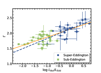
Figure 7: Hard X-ray photon index vs. $L_{\rm Bol}/L_{\rm Edd}$ for the super-Eddington subsample (blue circles) and the sub-Eddington subsample (green squares). The two subsamples overlap slightly in the $L_{\rm Bol}/L_{\rm Edd}$ values, because they are classified on the basis of $\dot{\rm\mathscr{M}}$ instead of $L_{\rm Bol}/L_{\rm Edd}$. The blue dashed (orange solid) line shows the best-fit relation for the super-Eddington subsample (full sample), given by Equation 8 (Equation 9).

We also investigated the correlations between $\Gamma$ and normalized accretion rate ($\dot{\rm\mathscr{M}}$; see Figure 8). Similar to the trends between $\Gamma$ and $L_{\rm Bol}/L_{\rm Edd}$, $\Gamma$ and $\dot{\rm\mathscr{M}}$ are highly correlated for the full sample ($r_{s}=0.70$ and $p=5.55\times 10^{-8}$) or the super-Eddington subsample ($r_{s}=0.63$ and $p=0.002$), but the correlation is not statistically significant for the sub-Eddington subsample ($r_{s}=0.14$ and $p=0.493$). For the super-Eddington subsample, the best-fit relation is

$$\Gamma=(0.19\pm 0.08){\rm log}\dot{\rm\mathscr{M}}+(1.85\pm 0.11),$$ (10)

with a scatter of 0.14. For the full sample, the best-fit relation obtained from the linear regression analysis is

$$\Gamma=(0.15\pm 0.02){\rm log}\dot{\rm\mathscr{M}}+(1.91\pm 0.03).$$ (11)

The similar dependences of $\Gamma$ on $L_{\rm Bol}/L_{\rm Edd}$ and $\dot{\rm\mathscr{M}}$ indicate that $L_{\rm Bol}/L_{\rm Edd}$ and $\dot{\rm\mathscr{M}}$ are likely correlated. A Spearman rank correlation test indicates a highly significant correlation ($r_{s}=0.97$ and $p=4.66\times 10^{-29}$) between $L_{\rm Bol}/L_{\rm Edd}$ and $\dot{\rm\mathscr{M}}$. Our linear regression analysis on log($L_{\rm Bol}/L_{\rm Edd}$) and $\rm log\dot{\rm\mathscr{M}}$ resulted in a slope of $0.53$. Such a tight $L_{\rm Bol}/L_{\rm Edd}\textrm{--}\dot{\rm\mathscr{M}}$ relation has also been reported in Huang et al. (2020) for their quasar sample, where they found a power-law slope of $0.52$. This relation can be naturally explained by the dependence of the two parameters on $M_{\rm BH}$: $\dot{\rm\mathscr{M}}$ mainly depends on $M_{\rm BH}^{-2}$ (see Section 2.6), and $L_{\rm Bol}/L_{\rm Edd}$ is proportional to $M_{\rm BH}^{-1}$. Therefore, $L_{\rm Bol}/L_{\rm Edd}$ and $\dot{\rm\mathscr{M}}$ are related in the form of $L_{\rm Bol}/L_{\rm Edd}\propto\dot{\rm\mathscr{M}}^{0.5}$, with some scatter associated with the distributions of $L_{\rm Bol}$ and $L_{2500~{}{\textup{\AA}}}$ for the sample AGNs. Given the similarities of the $\Gamma\textrm{--}L_{\rm Bol}/L_{\rm Edd}$ and $\Gamma\textrm{--}\dot{\rm\mathscr{M}}$ relations, we focus on the $\Gamma\textrm{--}L_{\rm Bol}/L_{\rm Edd}$ relations in the following discussion.

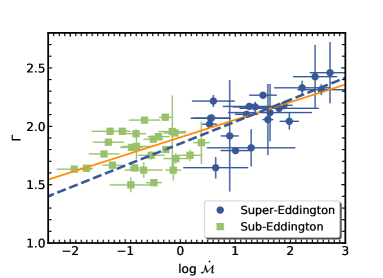
Figure 8: Hard X-ray photon index vs. normalized accretion rate for the super-Eddington subsample (blue circles) and the sub-Eddington subsample (green squares). The blue dashed (orange solid) line shows the best-fit relation for the super-Eddington subsample (full sample), given by Equation 10 (Equation 11).

3.4 Spectral Energy Distributions of Super-Eddington Accreting AGNs

We constructed IR-to-X-ray SEDs for ten super-Eddington accreting AGNs with UV luminosities ($\nu L_{\nu}|_{\lambda=2500~{}\textup{\AA}}$) exceeding $10^{44.5}\ \rm erg~{}s^{-1}$. This selection is based on the consideration that the contamination from host galaxies should be small in luminous AGNs. The photometric data were collected from the Wide-field Infrared Survey Explorer (WISE; Wright et al., 2010), Two Micron All Sky Survey (2MASS; Skrutskie et al., 2006), SDSS, and GALEX public catalogs. The UV/optical data were corrected for Galactic extinction using the extinction law of Cardelli et al. (1989). The SEDs are shown in Figure 9. We added the OM or UVOT data and the 2 keV and 10 keV luminosities. For comparison, the mean SED of typical SDSS quasars from Krawczyk et al. (2013), scaled to the $2500~{}\textup{\AA}$ luminosity of each object, is plotted in each panel of Figure 9. The IR-to-X-ray SEDs of most objects are consistent with those of typical quasars, except for three objects (SDSS J$081441+212918$, PG $0844+349$, and PG $0953+414$) that show deficiencies in the mid-IR (WISE) bands.

The weak IR emission of PG  $0844+349$ and PG $0953+414$ has been reported in Lyu et al. (2017). PG $0953+414$ was identified as a warm-dust-deficient quasar, and PG $0844+349$ was an ambiguous case but likely a hot-dust-deficient quasar. The IR weakness of these three objects may be related to their super-Eddington accretion rates. As suggested by Kawakatu & Ohsuga (2011), super-Eddington accreting AGNs may tend to show weak IR emission due to the self-occultation effect of the thick accretion disk, which reduces the illumination of the torus. However, these three IR weak objects do not show extreme properties (e.g., $M_{\rm BH}$, $L_{\rm Bol}/L_{\rm Edd}$) compared to the other seven objects, and they also exhibit typical optical-to-X-ray SEDs. PG $0844+349$ has been found to show extreme X-ray variability (e.g., Gallagher et al., 2001; Gallo et al., 2011), but the other extremely X-ray variable AGN among these ten objects, PG $1211+143$, does not have IR deficiency. We thus do not find any distinctive feature that may be related to the IR deficiency. Further investigations, probably utilizing a larger SED sample, are required to confirm and understand the potential IR deficiency of super-Eddington accreting AGNs.

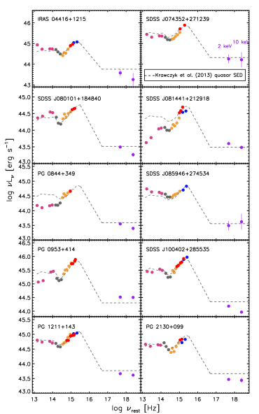
Figure 9: IR-to-X-ray SEDs for the ten super-Eddington accreting AGNs with log$(\nu L_{\nu})|_{\lambda=2500~{}\textup{\AA}}\geq 44.5$. The IR-to-UV photometric data points were gathered from the WISE (magenta), 2MASS (gray), SDSS (orange), and GALEX (blue) catalogs. The UVOT and OM photometric data are shown as red points, and the luminosities at 2 keV and 10 keV are shown as purple points. The dashed line in each panel shows the mean SED of SDSS quasars (Krawczyk et al., 2013), which is scaled to the mean $2500~{}{\textup{\AA}}$ luminosity extrapolated from the UV photometric data of each object. The SEDs may be affected by variability due to non-simultaneous multi-band observations (e.g., SDSS J$074352+271239$ and SDSS J$081441+212918$).

4 Discussion

4.1 X-ray Emission Strength of Super-Eddington Accreting AGNs

We examined the correlations between $\alpha_{\rm OX}$ and $L_{2500~{}{\textup{\AA}}}$ for the super- and sub-Eddington subsamples, in order to determine whether super-Eddington accreting AGNs show different X-ray emission strength relative to UV/optical emission, compared to sub-Eddington accreting AGNs. Significant $\alpha_{\rm OX}\textrm{--}L_{2500~{}{\textup{\AA}}}$ correlations were confirmed for both subsamples. Compared to the sub-Eddington subsample, the best-fit relation between $\alpha_{\rm OX}$ and ${\rm log}(L_{2500~{}{\textup{\AA}}})$ for the super-Eddington subsample has a slightly flatter slope and a smaller intercept, but the parameters are consistent considering the $1\sigma$ uncertainties. The two subsamples also show similar $\Delta\alpha_{\rm OX}$ distributions (see Figure 5), with the ranges within the rms scatter of the Steffen et al. (2006) $\alpha_{\rm OX}\textrm{--}L_{2500~{}{\textup{\AA}}}$ relation. These results suggest that super-Eddington accreting AGNs show normal X-ray emission strength and follow a similar $\alpha_{\rm OX}\textrm{--}L_{2500~{}{\textup{\AA}}}$ relation as sub-Eddington accreting AGNs or typical AGNs, when their high-state X-ray data are considered.

A few studies of IMBH candidates with high Eddington ratios have revealed that a large fraction of IMBHs deviate significantly (with $\Delta\alpha_{\rm OX}\lesssim-0.25$; corresponding to $\gtrsim 2\sigma$ deviations) from the $\alpha_{\rm OX}\textrm{--}L_{2500~{}{\textup{\AA}}}$ relation for typical AGNs (e.g., Greene & Ho, 2007; Dong et al., 2012). We consider that the X-ray weakness of these IMBHs may be caused by X-ray absorption, as some objects show unusually flat X-ray spectra. Our investigation shows that super-Eddington accreting AGNs tend to show strong X-ray variability, likely related to shielding by the thick accretion disk and/or its associated outflow in the low states (see discussion in Section 4.4 bellow). In this study, we have intentionally selected high-state observational data to probe the intrinsic X-ray properties of our sample. Mixing high- and low-state data could reveal a fraction of objects deviating from the expected $\alpha_{\rm OX}\textrm{--}L_{2500~{}{\textup{\AA}}}$ relation, showing different levels of X-ray weakness.

Equivalent to the $\alpha_{\rm OX}\textrm{--}L_{2500~{}{\textup{\AA}}}$ correlations, strong and consistent correlations between $L_{\rm 2~{}keV}$ and $L_{2500~{}{\textup{\AA}}}$ for the super- and sub-Eddington subsamples were also found. Although the $L_{\rm 2~{}keV}\textrm{--}L_{2500~{}{\textup{\AA}}}$ and $\alpha_{\rm OX}\textrm{--}L_{2500~{}{\textup{\AA}}}$ relations are strong, the scatters of the two relations are large, as also noted in previous studies (e.g., Vignali et al., 2003; Strateva et al., 2005; Steffen et al., 2006; Just et al., 2007; Lusso et al., 2010; Lusso & Risaliti, 2016). The scatters may be caused by factors such as measurement uncertainties, X-ray absorption, host-galaxy contamination, and intrinsic scatter related to differences in AGN physical properties (e.g., Lusso & Risaliti, 2016). There are only slight ($<1\sigma$) differences between the power-law slopes and intercepts of the $\alpha_{\rm OX}\textrm{--}L_{2500~{}{\textup{\AA}}}$ ($L_{\rm 2~{}keV}\textrm{--}L_{2500~{}{\textup{\AA}}}$) relation for the two subsamples, suggesting that the different accretion physics in super- and sub-Eddington accreting AGNs likely contributes little to the intrinsic scatter of these relations.

The $\alpha_{\rm OX}\textrm{--}L_{2500~{}{\textup{\AA}}}$ or $L_{\rm 2~{}keV}\textrm{--}L_{2500~{}{\textup{\AA}}}$ relation indicates that the fraction of accretion-disk radiation (or equivalently the accretion power in the radiatively-efficient case) dissipated via the corona has a strong dependence on the UV luminosity. More optically luminous AGNs are observed to produce relatively weaker X-ray emission from their coronae. There is still no clear understanding of the physics behind this empirical disk-corona connection. Simple qualitative explanations usually involve how the accretion power dissipation formula or the coronal size/structure changes with accretion rate (e.g., Merloni 2003; Wang et al. 2004; Yang et al. 2007; Lusso & Risaliti 2017; Kubota & Done 2018; Wang et al. 2019; Jiang et al. 2019; Arcodia et al. 2019; see more discussion in Section 4.2). Nevertheless, our finding here that super-Eddington accreting AGNs follow basically the same $\alpha_{\rm OX}\textrm{--}L_{2500~{}{\textup{\AA}}}$ ($L_{\rm 2~{}keV}\textrm{--}L_{2500~{}{\textup{\AA}}}$) relation as that for typical AGNs suggests that super-Eddington accreting AGNs, regardless of their geometrically thick accretion disks and the potential photon-trapping effects, likely share the same relation when dissipating the accretion power between the accretion disk and corona as sub-Eddington accreting AGNs. Alternatively, our finding may suggest that super-Eddington accreting AGNs, or at least the AGNs in our super-Eddington subsample, probably do not have distinctive accretion physics (e.g., no thick disks) compared to sub-Eddington accreting AGNs.

Our finding indicates that typical AGNs with ${\rm log}(L_{2500~{}{\textup{\AA}}})$ in the range of $\sim 27.3\textrm{--}30.6\ \rm(erg\ s^{-1}\ Hz^{-1})$ all follow the same $\alpha_{\rm OX}\textrm{--}L_{2500~{}{\textup{\AA}}}$ relation. After accounting for the scatter, this relation may indeed be used to estimate the intrinsic X-ray luminosity for an AGN/quasar given its UV/optical luminosity, and then to identify X-ray weak AGNs (e.g., Gibson et al. 2008; Pu et al. 2020) or to measure enhanced X-ray emission in radio-loud AGNs (e.g., Miller et al., 2011; Zhu et al., 2020).

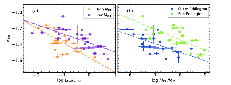
Figure 10: X-ray-to-optical power-law slope ($\alpha_{\rm OX}$) vs. (a) $L_{\rm Bol}/L_{\rm Edd}$ and (b) $M_{\rm BH}$. In Panel (a), the orange circles represent high-$M_{\rm BH}$ objects with BH masses larger than the median value ($10^{7.44}~{}M_{\odot}$) of the full sample, and the purple squares represent the low-$M_{\rm BH}$ objects. The best-fit relations for the high-$M_{\rm BH}$ objects (orange dashed line) and low-$M_{\rm BH}$ objects (purple dot-dashed line) are plotted to guide the eye. In Panel (b), the super-Eddington (sub-Eddington) subsample is shown as blue circles (green squares), with the best-fit relation shown as the blue dashed (green dot-dashed) line.

4.2 A More Fundamental $\alpha_{\rm OX}$ versus $L_{\rm Bol}/L_{\rm Edd}$ plus $M_{\rm BH}$ Relation?

Our carefully constructed sample of AGNs with the best available BH-mass measurements provides a good opportunity for seeking a physical explanation of the observed $\alpha_{\rm OX}\textrm{--}L_{2500~{}{\textup{\AA}}}$ relation. In this section, we explore the possibility that the $\alpha_{\rm OX}\textrm{--}L_{2500~{}{\textup{\AA}}}$ relation is physically driven by the dependences of $\alpha_{\rm OX}$ on the two fundamental parameters, $L_{\rm Bol}/L_{\rm Edd}$ and $M_{\rm BH}$ (e.g., Shemmer et al., 2008).

One promising explanation for the formation of the corona is that the magnetic field amplified by the magneto-rotational instability (MRI) saturates due to vertical buoyancy, and it extends outside the accretion disk and forms a magnetically dominated coronal region (e.g., Stella & Rosner, 1984; Tout & Pringle, 1992; Svensson & Zdziarski, 1994; Miller & Stone, 2000; Merloni & Fabian, 2002; Blackman & Pessah, 2009; Jiang et al., 2014). A fraction ($f_{\rm X}$) of the accretion power carried away by the magnetic buoyancy is released via magnetic reconnection, thereby heating the corona (e.g., Galeev et al., 1979; Di Matteo, 1998; Liu et al., 2002; Uzdensky & Goodman, 2008). Based on these descriptions and the basic theory of the standard accretion disk (Shakura & Sunyaev, 1973), analytic models of the accretion disk-corona system (e.g., Merloni, 2003; Wang et al., 2004; Yang et al., 2007; Cao, 2009; Lusso & Risaliti, 2017; Kubota & Done, 2018; Wang et al., 2019; Arcodia et al., 2019; Cheng et al., 2020) predict a smaller energy dissipation fraction $f_{\rm X}$ for an accretion disk with a higher $L_{\rm Bol}/L_{\rm Edd}$, as the accretion disk becomes more radiation-pressure dominated and the MRI grows less rapidly. Besides, the radiation magneto-hydrodynamic (MHD) simulations by Jiang et al. (2014, 2019) also suggest a weaker (smaller $f_{\rm X}$) and more compact corona when the accretion rate increases. A similar, albeit weaker, trend between $f_{\rm X}$ and $M_{\rm BH}$ is also expected (e.g., Figure 5 of Yang et al., 2007), as the gas pressure decreases more rapidly than the radiation pressure when $M_{\rm BH}$ increases and the disk is again more radiation-pressure dominated with relatively weaker MRI.

The parameter $\alpha_{\rm OX}$, as an indicator of the coronal X-ray emission strength relative to accretion-disk UV/optical emission, is likely dependent on the fraction of accretion energy released in the corona. As discussed above, an AGN with higher $L_{\rm Bol}/L_{\rm Edd}$ and/or $M_{\rm BH}$ has a smaller $f_{\rm X}$, and thus the corona is relatively weaker, leading to a smaller (steeper) $\alpha_{\rm OX}$. Therefore, $\alpha_{\rm OX}$ is expected to be inversely correlated with $L_{\rm Bol}/L_{\rm Edd}$ or $M_{\rm BH}$ when the other parameter is fixed. We thus investigated whether these expected correlations exist for our sample. It is shown in Figure 10(a) that $\alpha_{\rm OX}$ is anti-correlated with $L_{\rm Bol}/L_{\rm Edd}$, and the correlation appears more significant when breaking the full sample into the high-$M_{\rm BH}$ and low-$M_{\rm BH}$ subsamples. Moreover, at a fixed $L_{\rm Bol}/L_{\rm Edd}$, objects with higher $M_{\rm BH}$ systematically have lower $\alpha_{\rm OX}$, which implies a dependence of $\alpha_{\rm OX}$ on $M_{\rm BH}$. Such an anti-correlation does exist, as shown in Figure 10(b). The correlation appears more significant when limiting to the super-Eddington or sub-Eddington subsample. We performed partial correlation analysis using the R package ppcor (Kim, 2015) on $\alpha_{\rm OX}$ versus $L_{\rm Bol}/L_{\rm Edd}$ ($M_{\rm BH}$), controlling for $M_{\rm BH}$ ($L_{\rm Bol}/L_{\rm Edd}$). The $\alpha_{\rm OX}\textrm{--}L_{\rm Bol}/L_{\rm Edd}$ ($\alpha_{\rm OX}\textrm{--}M_{\rm BH}$) correlation is highly significant when controlling for $M_{\rm BH}$ ($L_{\rm Bol}/L_{\rm Edd}$), with a Spearman correlation coefficient of $-0.74$ ($-0.69$) and a $p$-value of $3.00\times 10^{-9}$ ($1.11\times 10^{-7}$). The dependence of $\alpha_{\rm OX}$ on $L_{\rm Bol}/L_{\rm Edd}$ or $M_{\rm BH}$ has been discussed in previous studies. Some authors found a significant correlation between $\alpha_{\rm OX}$ and $L_{\rm Bol}/L_{\rm Edd}$ (e.g., Shemmer et al., 2008; Grupe et al., 2010; Lusso et al., 2010; Wu et al., 2012; Jin et al., 2012; Chiaraluce et al., 2018), while some found no significant correlation (e.g., Vasudevan & Fabian, 2007; Done et al., 2012). Some authors found a significant correlation between $\alpha_{\rm OX}$ and $M_{\rm BH}$ (e.g., Done et al., 2012; Chiaraluce et al., 2018). Our results above suggest that $\alpha_{\rm OX}$ likely depends on both $L_{\rm Bol}/L_{\rm Edd}$ and $M_{\rm BH}$. Thus the scatter of the correlation with solely $L_{\rm Bol}/L_{\rm Edd}$ or $M_{\rm BH}$ is considerable.

Figure 11: (a) $\alpha_{\rm OX}\textrm{--}L_{\rm Bol}/L_{\rm Edd}\textrm{--}M_{\rm BH}$ plane seen edge-on. The red solid line shows the best-fit relation given by Equation 12. (b) $\alpha_{\rm OX}$ vs. $2500\textup{\AA}$ luminosity. The red solid line shows the best-fit relation given by Equation 4. The bottom panels show the fitting residuals, defined as the differences between the observed $\alpha_{\rm OX}$ values and the expectations from the corresponding best-fit relation. The two relations show comparable scatters.

We performed multi-variate linear regression on the relation $\alpha_{\rm OX}=\beta{\rm log}(L_{\rm Bol}/L_{\rm Edd})+\gamma{\rm log}M_{\rm BH}+\delta$ using the Python package emcee (Foreman-Mackey et al., 2013), which is a Python implementation of Goodman & Weare’s affine-invariant Markov chain Monte Carlo (MCMC) ensemble sampler. The measurement uncertainties on the three parameters are included in the fitting. The best-fit relation is

$$\alpha_{\rm OX}=(-0.13\pm 0.01){\rm log}(L_{\rm Bol}/L_{\rm Edd})-$$

$$(0.10\pm 0.01){\rm log}M_{\rm BH}-(0.69\pm 0.09)$$ (12)

with a scatter of 0.07. An edge-on view of the $\alpha_{\rm OX}\textrm{--}L_{\rm Bol}/L_{\rm Edd}\textrm{--}M_{\rm BH}$ three-dimensional plane is shown in Figure 11(a). The $\alpha_{\rm OX}\textrm{--}L_{\rm Bol}/L_{\rm Edd}\textrm{--}M_{\rm BH}$ relation may be the physical origin of the observed $\alpha_{\rm OX}\textrm{--}L_{2500\textup{\AA}}$ relation, as $L_{\rm Bol}/L_{\rm Edd}\times M_{\rm BH}\propto L_{\rm Bol}\propto L_{2500\textup{\AA}}$. For comparison, we plotted the $\alpha_{\rm OX}$ versus ${\rm log}(L_{\rm 2500~{}\textup{\AA}})$ relation for our full sample in Figure 11(b). We note that the scatter of the $\alpha_{\rm OX}\textrm{--}L_{\rm Bol}/L_{\rm Edd}\textrm{--}M_{\rm BH}$ relation is comparable to that of the $\alpha_{\rm OX}\textrm{--}L_{2500\textup{\AA}}$ relation, which is probably due to the large uncertainties on both $L_{\rm Bol}/L_{\rm Edd}$ and $M_{\rm BH}$. It could also be due to the dependence of $\alpha_{\rm OX}$ on a third parameter, the ratio of the gas plus radiation pressure to the magnetic pressure, as this ratio may work together with $L_{\rm Bol}/L_{\rm Edd}$ and $M_{\rm BH}$ to determine the broad-band AGN SED (e.g., Cheng et al., 2020).

We note that it is difficult to determine if the relation between $\alpha_{\rm OX}$ and $L_{\rm Bol}/L_{\rm Edd}$ plus $M_{\rm BH}$ is more fundamental than the $\alpha_{\rm OX}\textrm{--}L_{\rm 2500~{}\textup{\AA}}$ relation, or if it is a secondary manifestation of the observed $\alpha_{\rm OX}\textrm{--}L_{\rm 2500~{}\textup{\AA}}$ relation. There is a tight linear correlation ($r_{s}\approx 1$) between $L_{\rm Bol}$ ($\propto L_{\rm Bol}/L_{\rm Edd}\times M_{\rm BH}$) and $L_{\rm 2500~{}\textup{\AA}}$ for our sample objects. Therefore, from the $\alpha_{\rm OX}\textrm{--}L_{\rm 2500~{}\textup{\AA}}$ relation (equivalently an $\alpha_{\rm OX}\textrm{--}L_{\rm Bol}$ relation), a significant partial correlation between $\alpha_{\rm OX}$ and $L_{\rm Bol}/L_{\rm Edd}$ or $M_{\rm BH}$ when controlling for the other parameter is expected. We performed a test through creating mock sets of parameter $K$ to replace $M_{\rm BH}$. In each realization, the $K$ values are randomly distributed in the same range as that of $M_{\rm BH}$ for our sample, and we then analyzed the partial correlation between $\alpha_{\rm OX}$ and $L_{\rm 2500~{}\textup{\AA}}/K$ when controlling for $K$. A number of realizations with different $K$ values generated correlation coefficients of $-0.6$ to $-0.8$ and $p$-values of $10^{-7}\textrm{--}10^{-9}$. These correlation significance levels are similar to those of $\alpha_{\rm OX}$ against $L_{\rm Bol}/L_{\rm Edd}$ or $M_{\rm BH}$. Plots of $\alpha_{\rm OX}$ versus $L_{\rm 2500~{}\textup{\AA}}/K$ are also similar to the $\alpha_{\rm OX}\textrm{--}L_{\rm Bol}/L_{\rm Edd}$ relation presented in Figure 10 (a). Therefore, we cannot determine whether the $\alpha_{\rm OX}$ versus $L_{\rm Bol}/L_{\rm Edd}$ plus $M_{\rm BH}$ correlation is fundamental, although physically this is an appealing explanation. A possible method to resolve this issue is to investigate these correlations for individual AGNs, such as changing-look AGNs varying in accretion rate. Without the complication from $M_{\rm BH}$, we may constrain better the dependence of $\alpha_{\rm OX}$ on $L_{\rm Bol}/L_{\rm Edd}$.

4.3 Relation between $\Gamma$ and $L_{\rm Bol}/L_{\rm Edd}$

A strong correlation between $\Gamma$ and $L_{\rm Bol}/L_{\rm Edd}$ ($\dot{\rm\mathscr{M}}$) was confirmed for our full sample and super-Eddington subsample. However, such a correlation is not statistically significant for the sub-Eddington subsample. We caution that large uncertainties associated with the measurements of $L_{\rm Bol}/L_{\rm Edd}$ and $\Gamma$ may introduce considerable uncertainties for the $\Gamma\textrm{--}{\rm log}(L_{\rm Bol}/L_{\rm Edd})$ relation. The BH masses of our sample were obtained from the RM method, which is arguably the most reliable method for AGN BH-mass measurements. However, the RM method is based on the assumption of virial gas motions in the broad-line regions (BLRs), which may not be valid for super-Eddington accreting systems due to the impact of the large radiation pressure and the anisotropy of the ionizing radiation (e.g., Marconi et al., 2008, 2009; Netzer & Marziani, 2010; Krause et al., 2011; Pancoast et al., 2014; Li et al., 2018). In addition, there are potential uncertainties associated with the measurements of $L_{\rm Bol}$. The approach we used to obtain $L_{\rm Bol}$ is similar to the estimation through the use of bolometric corrections, which employ approximations to the mean properties of typical quasars. The main improvement in our study is that the X-ray spectral shapes for individual objects were taken into account. Additional uncertainties on $L_{\rm Bol}$ may come from the UV-to-X-ray SED which was set to a simple power law. Super-Eddington accreting AGNs are expected to emit excess EUV radiation compared to sub-Eddington accreting AGNs (e.g., Castelló-Mor et al., 2016; Kubota & Done, 2018), although there is still no clear observational evidence due to the lack of EUV data. Moreover, the criterion of $L_{\rm Bol}/L_{\rm Edd}$ (or $\dot{\rm\mathscr{M}}$) for identifying super-Eddington accreting AGNs is also rather uncertain (e.g., Laor & Netzer, 1989; Sa̧dowski et al., 2011; Sa̧dowski & Narayan, 2016).

The choice of X-ray energy band in spectral fitting may also introduce uncertainties on the derived photon indices. The X-ray energy band investigated in this study is the rest-frame $>\rm 2~{}keV$ band. This choice is based on the idea that the X-ray spectrum in this band is generally insensitive to contamination from the potential soft-excess component or absorption (e.g., Shemmer et al., 2006, 2008; Risaliti et al., 2009; Brightman et al., 2013). However, although there is no clear evidence of soft excesses and absorption in the hard X-ray spectra of our sample AGNs, their influence might not be completely eliminated.

With the above caveats in mind, we do find a significant $\Gamma\textrm{--}L_{\rm Bol}/L_{\rm Edd}$ relation for the full sample. Compared to similar relations reported in previous studies (see Section 3.3), there are notable discrepancies in the power-law slopes. These discrepancies might be due to the different samples, different $M_{\rm BH}$ ($L_{\rm Bol}/L_{\rm Edd}$) estimation methods, or different statistical methods used in these studies (also see Section 4.3 of Brandt & Alexander 2015). A large unbiased sample with reliable parameter measurements and covering a wide range of $L_{\rm Bol}/L_{\rm Edd}$ is required to establish the $\Gamma\textrm{--}L_{\rm Bol}/L_{\rm Edd}$ relation for general AGNs. The X-ray photon index could then, if confirmed, serve as an Eddington-ratio indicator, provided that the large scatter of the $\Gamma\textrm{--}L_{\rm Bol}/L_{\rm Edd}$ relation is understood and taken into account.

There is not a significant $\Gamma\textrm{--}L_{\rm Bol}/L_{\rm Edd}$ correlation for the sub-Eddington subsample. The best-fit relation for the super-Eddington subsample does not appear to differ significantly from that for the full sample either. Therefore, we cannot constrain any difference between the super- and sub-Eddington accreting AGNs in terms of the $\Gamma\textrm{--}L_{\rm Bol}/L_{\rm Edd}$ relation. However, a few recent studies have reported that super-Eddington accreting AGNs have even steeper X-ray photon indices in excess of those expected from the $\Gamma\textrm{--}L_{\rm Bol}/L_{\rm Edd}$ relation for sub-Eddington accreting AGNs (e.g., Gliozzi & Williams, 2020; Huang et al., 2020). If such a finding is real, any physical explanations must involve the expected properties of super-Eddington accretion disks, while maintaining basically the same accretion power dissipation relation for the accretion disk-corona system (see the discussion in Section 4.1). A possible physical explanation is that in the thick disk of a super-Eddington AGN, more radiation is emitted from the inner region of the disk due to the longer diffusion timescale for photons to escape from the disk surface and the stronger magnetic buoyancy in the inner region (e.g., Jiang et al., 2014); this effect increases the UV/optical emission received by the compact corona, reduces its temperature and optical depth, and leads to an even steeper X-ray spectrum. Nevertheless, a larger sample of sub-Eddington accreting AGNs with RM measurements is required to allow further investigations of any difference between the $\Gamma\textrm{--}L_{\rm Bol}/L_{\rm Edd}$ correlations for super- and sub-Eddington accreting AGNs.

4.4 The Impact of X-ray Variability

Our study suggests that super-Eddington accreting AGNs exhibit normal X-ray emission and generally follow the same $\alpha_{\rm OX}\textrm{--}L_{2500~{}{\textup{\AA}}}$ ($L_{\rm 2~{}keV}\textrm{--}L_{2500~{}{\textup{\AA}}}$) relation as sub-Eddington accreting AGNs, as long as their intrinsic X-ray emission is considered. However, a fraction of super-Eddington accreting AGNs tend to show extreme large-amplitude (factors of $>10$) X-ray variability (e.g., 1H $0707-495$: Fabian et al. 2012; IRAS $13224-3809$: Boller et al. 1997; Jiang et al. 2018; SDSS J$075101.42+291419.1$: Liu et al. 2019). Three super-Eddington accreting AGNs (Mrk 335, PG $1211+143$, and PG $0844+349$) in our sample have varied in X-ray flux by factors of larger than 10, while they have not shown coordinated UV/optical continuum or emission-line variability (e.g., Guainazzi et al., 1998; Peterson et al., 2000; Grupe et al., 2007; Bachev et al., 2009; Gallo et al., 2011; Grupe et al., 2012; Gallo et al., 2018). In their low X-ray states, they inevitably deviate significantly from the expected $\alpha_{\rm OX}\textrm{--}L_{2500~{}{\textup{\AA}}}$ ($L_{\rm 2~{}keV}\textrm{--}L_{2500~{}{\textup{\AA}}}$) relation. Their low X-ray states can be explained by a partial-covering absorption scenario, where the geometrically inner thick accretion disk and its associated outflow play the role of the absorber (see Luo et al., 2015; Liu et al., 2019; Ni et al., 2020, and references therein). Analyses of their low-state spectra sometimes cannot detect any absorption, perhaps because they exhibit soft $\approx 0.3\textrm{--}6$ keV X-ray spectra, which are probably dominated by the soft-excess component or the transmitted fraction of X-ray emission unaffected by the partial covering absorber (see the case of SDSS $\rm J075101.42+291419.1$ in Liu et al., 2019).

The fraction of extremely X-ray variable AGNs among super-Eddington accreting AGNs was estimated to be $\sim 15\textrm{--}24\%$ (Liu et al., 2019). In this study, the three extremely X-ray variable AGNs constitute a fraction of $\approx 14\%$ (3/21) among the super-Eddington subsample, which is generally consistent with that reported in Liu et al. (2019). Moreover, a number of our super-Eddington accreting AGNs, mostly the SDSS quasars, have limited numbers (one or two) of X-ray observations, and thus their X-ray variability behavior is not well constrained. It is thus possible that the actual number of extremely X-ray variable AGNs among our sample is larger, resulting in a more significant impact of X-ray variability on the study of the $\alpha_{\rm OX}\textrm{--}L_{2500~{}{\textup{\AA}}}$ ($L_{\rm 2~{}keV}\textrm{--}L_{2500~{}{\textup{\AA}}}$) and $\Gamma\textrm{--}L_{\rm Bol}/L_{\rm Edd}$ relations for super-Eddington accreting AGNs. We therefore emphasize the importance of using high-state X-ray data to probe the intrinsic accretion disk-corona connections in AGNs, especially for objects with high accretion rates. Multiple X-ray observations are required to collect the variability information for every sample object, in order to construct an unbiased sample for such studies.

5 Summary and Future Prospects

In this study, we constructed a sample of 47 AGNs with RM measurements, to systematically study the observational differences between the coronae and accretion disk-corona connections in super- and sub-Eddington accreting AGNs. All our sample objects have sensitive X-ray coverage from archival XMM-Newton, Chandra, or Swift observations, and we have selected high-state data for objects with multiple observations to probe their intrinsic X-ray emission. All the sample objects, except one, have simultaneous UV/optical data. Our full sample was divided into the super-Eddington subsample with $\dot{\rm\mathscr{M}}\geq 3$ and sub-Eddington subsample with $\dot{\rm\mathscr{M}}<3$, and we performed detailed statistical analysis on the $\alpha_{\rm OX}(L_{\rm 2~{}keV})\textrm{--}L_{2500~{}{\textup{\AA}}}$ and $\Gamma\textrm{--}L_{\rm Bol}/L_{\rm Edd}(\dot{\rm\mathscr{M}})$ correlations for the two subsamples. Our main results are as follows:

1. We found a strong correlation between $\alpha_{\rm OX}$ and $L_{2500~{}{\textup{\AA}}}$ for both the super- and sub-Eddington subsamples. The linear regression analysis on $\alpha_{\rm OX}$ versus ${\rm log}L_{2500~{}{\textup{\AA}}}$ reveals a slope of $-0.106\pm 0.019$ for the super-Eddington subsample, which is slightly flatter than, but still consistent within $1\sigma$ with the slope of $-0.111\pm 0.019$ for the sub-Eddington subsample. The best-fit intercepts are also consistent within $1\sigma$. A strong correlation between $L_{\rm 2~{}keV}$ and $L_{2500~{}{\textup{\AA}}}$ for both the super- and sub-Eddington subsamples was also found. The best-fit ${\rm log}(L_{\rm 2~{}keV})\textrm{--}{\rm log}(L_{2500~{}{\textup{\AA}}})$ relations for the two subsamples are also consistent considering the $1\sigma$ uncertainties. See Section 3.1.

2. A statistically significant correlation was found between the hard (rest-frame $>2$ keV) X-ray spectral photon index ($\Gamma$) and $L_{\rm Bol}/L_{\rm Edd}$ for the super-Eddington subsample and the full sample. However, there is no significant correlation between $\Gamma$ and $L_{\rm Bol}/L_{\rm Edd}$ for the sub-Eddington subsample. The slope of the best-fit $\Gamma\textrm{--}{\rm log}(L_{\rm Bol}/L_{\rm Edd})$ relation for the super-Eddington subsample is $0.33\pm 0.13$. See Section 3.3.

3. We constructed IR-to-X-ray SEDs for ten super-Eddington accreting AGNs with $2500~{}{\textup{\AA}}$ luminosities exceeding $10^{44.5}~{}\rm erg~{}s^{-1}$. The SEDs of most objects are largely consistent with those of typical quasars, except for three objects that show weaker mid-IR emission. See Section 3.4.

4. Super- and sub-Eddington accreting AGNs follow the same $\alpha_{\rm OX}\textrm{--}L_{2500~{}{\textup{\AA}}}$ ($L_{\rm 2~{}keV}\textrm{--}L_{2500~{}{\textup{\AA}}}$) relation, indicating that super-Eddington accreting AGNs are not significantly X-ray weak compared to sub-Eddington accreting AGNs, as long as their intrinsic X-ray emission is considered. These two groups likely share the same accretion power dissipation relation for the accretion disk-corona system. See Section 4.1.

5. We discuss the possibility that the $\alpha_{\rm OX}$ versus $L_{\rm Bol}/L_{\rm Edd}$ plus $M_{\rm BH}$ relation serves as the physical driver for the observed $\alpha_{\rm OX}\textrm{--}L_{2500~{}{\textup{\AA}}}$ relation. Significant dependences of $\alpha_{\rm OX}$ on both $L_{\rm Bol}/L_{\rm Edd}$ and $M_{\rm BH}$ are confirmed for our sample. A multi-variate linear regression revealed the relation: $\alpha_{\rm OX}=(-0.13\pm 0.01){\rm log}(L_{\rm Bol}/L_{\rm Edd})-(0.10\pm 0.01){\rm log}M_{\rm BH}-(0.69\pm 0.09)$. See Section 4.2.

There is not a significant correlation between $\Gamma$ and $L_{\rm Bol}/L_{\rm Edd}$ for the sub-Eddington subsample, probably due to the small sample size. We thus cannot constrain the difference between the $\Gamma\textrm{--}L_{\rm Bol}/L_{\rm Edd}$ relations for the two subsamples. From our parent sample, we excluded another six objects without X-ray observations and six objects with low-S/N observations. Five of them have new Chandra observations, which will provide constraints on their X-ray properties in the near future. If targeted observations with XMM-Newton or Chandra are obtained for the other objects, we will have a larger sample after adding these 12 objects.

We may also consider a larger sample from some ongoing or upcoming AGN RM projects. For example, the ongoing SDSS-RM project is the first dedicated multi-object RM program, executed with the SDSS-III Baryon Oscillation Spectroscopic Survey (BOSS) spectrograph (e.g., Shen et al., 2015). The primary goal of this project is to obtain RM measurements for $\gtrsim 100$ quasars, which cover a wider luminosity and redshift range compared to previous RM AGN samples (e.g., Shen et al., 2016; Grier et al., 2017, 2019). This program is accompanied by a large XMM-Newton program (XMM-RM) that completes the X-ray coverage of the same field (Liu et al., 2020). However, we note that this XMM-Newton program has a limited number of observations with limited exposure times, and some quasars are not detected. These X-ray observations cannot provide tight constraints on the X-ray properties, and they might also be biased against X-ray weak/undetected objects. Targeted observations with higher-quality data are still required.

There are some upcoming multi-object RM campaigns. The SDSS-V Black Hole Mapper (BHM) will further extend the number of RM AGNs to an ”industrial scale” (Kollmeier et al., 2017). It will perform RM campaigns in a number of fields including three of the four Deep-Drilling Fields (DDFs; XMM-LSS, CDF-S, and COSMOS) of the Vera C. Rubin Observatory Legacy Survey of Space and Time (LSST), and the total number of RM AGNs is expected to be $>1000$. The 4-metre multi-Object Spectroscopic Telescope (4MOST) TiDES-RM program will perform RM campaigns on the four LSST DDFs (XMM-LSS, CDF-S, COSMOS, and ELAIS-S1), and it will target around 700 AGNs (Brandt et al., 2018; Swann et al., 2019). The additional high-quality photometry from LSST will improve the accuracy of measured BH masses and the number of reverberation-lag detections. Moreover, the four DDFs have good X-ray coverage from completed or ongoing XMM-Newton and Chandra observations (e.g., Chen et al. 2018; Ni Q. et al. in preparation). Therefore, these programs will provide promising RM AGN samples with high-quality multiwavelength data to study the accretion disk-corona connections in AGNs.

Some issues related to the multiwavelength properties of super-Eddington accreting AGNs remain unclear. These AGNs are expected to have different SEDs compared to sub-Eddington accreting AGNs, with the primary differences arising in the EUV band (e.g., Castelló-Mor et al., 2016; Kubota & Done, 2018). The upcoming Chinese Space Station Optical survey (CSS-OS; e.g., Zhan 2018) will perform a deep NUV to optical imaging survey utilizing the Multi-Channel Imager. It will provide rest-frame EUV photometric observations for a large sample of high-redshift AGNs, which are valuable for studying the difference between the SEDs of super- and sub-Eddington accreting AGNs.

Our investigation has suggested that super-Eddington accreting AGNs tend to show extreme X-ray variability. It is thus important to obtain the high-state or intrinsic X-ray data for super-Eddington accreting AGNs when studying the disk-corona connection in these systems. The nature of extreme X-ray variability in super-Eddington accreting AGNs is still not well understood. With the ongoing eROSITA (Merloni et al., 2012; Predehl, 2017) X-ray survey of AGNs, we will obtain more variability information for the super-Eddington accreting AGNs that have limited numbers of X-ray observations now. We will likely discover more sources with extreme X-ray variability. Nearby luminous AGNs with high-quality mulitwavelength data are optimal samples for examining the physical scenario for such extreme behavior (e.g., Liu et al., 2019). Moreover, a systematic monitoring program of a uniform AGN sample selected from the RM campaigns discussed above, is required to constrain better the occurrence rate of extreme X-ray variability in super-Eddington accreting AGNs.

We thank the referee, Belinda Wilkes, for helpful suggestions and detailed comments. We thank Pu  Du, Chen Hu, Jian-Min Wang, Qiusheng Gu, Yong Shi, and Zhiyuan Li for helpful discussions. H.L. and B.L. acknowledge financial support from the National Natural Science Foundation of China grants 11991053 and 11673010 and National Key R&D Program of China grant 2016YFA0400702. H.L. acknowledges financial support from the program of China Scholarships Council (No. 201906190104) for her visit to the Pennsylvania State University. W.N.B. and J.D.T acknowledge support from NASA ADP grant 80NSSC18K0878. S.C.G. thanks the Natural Science and Engineering Research Council of Canada for support.

In this section, we give notes on individual objects showing strong variability in the X-ray and/or UV/optical bands.

Appendix A Mrk 335

Mrk 335, classified as a super-Eddington accreting AGN, is a well-studied bright AGN that was discovered to fall into a historically low X-ray state in 2007, with the flux dropping by a factor of $\sim 30$ compared to the 2000 and 2006 XMM-Newton fluxes (Grupe et al., 2007). Since then, it has been continuously monitored by Swift, but it has never fully recovered to the previous bright state (e.g., Grupe et al., 2008, 2012; Gallo et al., 2018). Compared to the 2000 XMM-Newton observation, the 2–10 keV X-ray flux of the 2006 XMM-Newton observation is slightly larger, and the exposure time is much longer (Grupe et al., 2008). We thus used the 2006 XMM-Newton data of Mrk 335 for our study.

Appendix B IRAS F$12397+3333$

IRAS F$12397+3333$, a super-Eddington accreting AGN, was observed by XMM-Newton in two consecutive revolutions during 2005 June 20 and 23, and the X-ray flux varied mildly between these two segments. The observations reveal that it was affected by ionized absorption mainly in the soft (rest-frame $<2$ keV) X-ray emission (Dou et al., 2016). Our simple power-law fitting of the rest-frame $>2~{}\rm keV$ spectrum yields a steep photon index of $\Gamma=2.15\pm 0.02$, consistent with that reported in Dou et al. (2016). It has a Chandra observation in 2000 (Observation ID: 3000). The rest-frame 2–7 keV Chandra spectrum is well modeled by a flatter power law with $\Gamma=1.30\pm 0.06$. The 2–10 keV flux of the Chandra observation is slightly smaller than those of the XMM-Newton observations, and the 0.5–2 keV flux is about half of the XMM-Newton fluxes. Therefore, the ionized absorption during the Chandra observation is likely stronger. We thus used the high-state XMM-Newton observation in our study.

The UV/optical spectrum of IRAS F$12397+3333$ appears to be affected by intrinsic reddening, based on the Balmer decrements of $\rm H\alpha/H\beta=5.71$ and 6.14 for the broad and narrow lines, respectively (e.g., Du et al., 2014). We found an unusual flattening of the optical/UV spectral slope at shorter wavelengths for the OM UV/optical fluxes, which also indicates intrinsic reddening. In order to correct for the intrinsic reddening, we converted the Balmer decrement of the broad lines to $E_{\rm B-V}$ assuming an intrinsic $\rm H\alpha/H\beta=3.06$ (Dong et al., 2008) and a Galactic extinction curve (Cardelli et al., 1989). The estimated $E_{\rm B-V}$ value is 0.59. We note that the extinction does not affect the hard X-ray emission of IRAS F$12397+3333$ (see Section 2.5)

Appendix C Mrk 382

Mrk 382, a super-Eddington accreting AGN, was observed by Chandra for 4.9 ks on 2010 December 6 (Observation ID: 13008). The rest-frame 2–7 keV Chandra spectrum is well described by a Galactic absorption modified power law with $\Gamma=1.25\pm 0.16$. The extrapolation of this power law to the 0.5–7 keV energy range reveals a small excess below 2 keV. In comparison, the rest-frame $>2$ keV XMM-Newton spectrum (observed on 2011 November 2) is much steeper ($\Gamma=2.17\pm 0.02$), with the 2–10 keV flux slightly larger than that of the Chandra observation. The $0.3\textrm{--}2/(1+z)$ keV XMM-Newton spectrum can be well fitted with a single power-law model ($\Gamma_{\rm s}=2.66\pm 0.01$) modified by Galactic absorption. The 0.5–2 keV flux was measured to be $4.89\times 10^{-12}\ \rm erg\ cm^{-2}\ s^{-1}$, larger than the Chandra 0.5–2 keV flux ($6.11\times 10^{-13}\rm erg\ cm^{-2}\ s^{-1}$) by a factor of about eight. Moreover, we have analyzed two archival Swift observations (2009 February 6 and 2011 September 12, respectively), which reveal fluxes between those in the Chandra and XMM-Newton observations. We thus considered the 2011 XMM-Newton observation as the high-state observation.

Appendix D Mrk 493

Mrk 493 is a super-Eddington accreting AGN. Bonson et al. (2018) has reported that the flux of Mrk 493 observed in the 2015 XMM-Newton observation is about half of that of the 2003 XMM-Newton observation. Mrk 493 also has one Chandra observation (2010 February 7; Dong et al. 2012), during which the flux and spectral photon index are consistent with those of the 2003 XMM-Newton observation. We thus used the 2003 XMM-Newton observation in our analysis.

Appendix E PG $1211+143$

PG $1211+143$, classified as a super-Eddington accreting AGN, is also well known for its extreme X-ray variability and spectral complexity, and it is an archetypical case of an AGN exhibiting an ultra-fast outflow (e.g., Pounds et al., 2003; Bachev et al., 2009; de Marco et al., 2011; Pounds et al., 2016; Lobban et al., 2016; Reeves et al., 2018). We analyzed additional XMM-Newton and Swift archival observations that have not been reported in the literature, and compared the derived X-ray fluxes with those reported in the aforementioned studies. We finally selected the highest-state observation (Observation ID: 0745110601) of the continuous XMM-Newton observations in 2014 (see e.g., Lobban et al., 2016).

Appendix F PG $0844+349$

PG $0844+349$ is a super-Eddington accreting AGN showing extreme X-ray variability by a factor of larger than 10, and its long-term X-ray light curve was presented in Gallo et al. (2011). The observation used in this study is its 2001 high-state XMM-Newton observation.

Appendix G Mrk 1310

Mrk 1310 is a sub-Eddington accreting AGN that has been observed multiple times by XMM-Newton and Swift from 2006 to 2019. Its X-ray flux showed extreme variability with a maximum amplitude of $\sim$ 30. Meanwhile, coordinated variability in UV/optical and IR fluxes was also observed, with smaller variability amplitudes toward longer wavelengths. Its optical spectral type has also changed, which makes it a changing-look AGN. The detailed analysis on this source will be reported in Luo B. et al. (in preparation). In this study, we used its 2016 Swift observation when it exhibited the brightest multiwavelengh fluxes.

Appendix H NGC 2617

NGC 2617 is a sub-Eddington accreting AGN that underwent a dramatic X-ray outburst from 2013 April to May, during which its X-ray flux increased by an order of magnitude, followed by an increase of the UV/ optical flux by almost an order of magnitude (e.g., Shappee et al., 2014; Giustini et al., 2017). Its optical spectral type switched from Seyfert 1.8 to Seyfert 1.0 due to the appearance of broad optical emission lines. It was observed by XMM-Newton on 2013 May 24 when its X-ray flux was at the peak level (see Figure 4 of Shappee et al., 2014). We thus used this observation in our study.

Appendix I Arp 151

Arp 151 is a sub-Eddington accreting AGN that showed normal X-ray emission in its 2009 February 15 Swift observation. The 0.3–10 keV spectrum can be well fitted by a single power-law model modified by Galactic absorption with $\Gamma=1.62\pm 0.09$, and the 0.5–2 keV flux was measured to be $4.80\times 10^{-12}~{}\rm erg\ cm^{-2}\ s^{-1}$. It was observed by Chandra on 2011 December 4 (Observation ID: 12871), when it exhibited a flatter 0.5–7 keV spectrum with $\Gamma=1.25\pm 0.02$. The 0.5–2 keV flux ($1.47\times 10^{-12}~{}\rm erg\ cm^{-2}\ s^{-1}$) decreased by a factor of $\approx 3$, compared to the Swift flux. We thus used the Swift observation in our study.

Table 1: BH Masses, Accretion Rates, and Optical Properties

Object	$z$	$E_{\rm B-V}$	$N_{\rm H,gal}$	log $L_{\rm 5100~{}{\textup{\AA}}}$	FWHM($\rm H\beta$)	log($M_{\rm BH}/M_{\odot}$)	log $\rm\dot{\mathscr{M}}$	log $L_{\rm Bol}$	log $L_{\rm Bol}/L_{\rm Edd}$
			($\rm 10^{20}\ cm^{-2}$)	($\rm erg\ s^{-1}$)	($\rm km\ s^{-1}$)			($\rm erg\ s^{-1}$)
(1)	(2)	(3)	(4)	(5)	(6)	(7)	(8)	(9)	(10)
Super-Eddington Subsample ($\rm\dot{\mathscr{M}}\geq 3$)
Mrk $335$	$0.026$	$0.035$	$3.48$	$43.76$	$1707$	$6.93^{+0.10}_{-0.11}$	$1.20^{+0.22}_{-0.20}$	$44.88$	$-0.23^{+0.11}_{-0.10}$
Mrk $1044$	$0.016$	$0.033$	$3.10$	$43.10$	$1178$	$6.45^{+0.12}_{-0.13}$	$1.50^{+0.26}_{-0.24}$	$44.48$	$-0.15^{+0.13}_{-0.12}$
IRAS $04416+1215$	$0.089$	$0.436$	$12.43$	$44.47$	$1522$	$6.78^{+0.31}_{-0.06}$	$2.72^{+0.11}_{-0.62}$	$45.52$	$0.57^{+0.08}_{-0.32}$
SDSS J$074352.02+271239.5$	$0.252$	$0.045$	$4.69$	$45.37$	$3156$	$7.93^{+0.05}_{-0.04}$	$1.59^{+0.09}_{-0.10}$	$46.32$	$0.21^{+0.10}_{-0.10}$
Mrk $382$	$0.034$	$0.048$	$4.81$	$43.12$	$1462$	$6.50^{+0.19}_{-0.29}$	$1.25^{+0.58}_{-0.38}$	$44.38$	$-0.29^{+0.29}_{-0.19}$
SDSS J$080101.41+184840.7$	$0.140$	$0.032$	$2.53$	$44.27$	$1930$	$6.78^{+0.34}_{-0.17}$	$2.22^{+0.34}_{-0.67}$	$45.31$	$0.35^{+0.17}_{-0.34}$
SDSS J$081441.91+212918.5$	$0.163$	$0.039$	$3.50$	$43.96$	$1729$	$7.18^{+0.20}_{-0.20}$	$1.36^{+0.40}_{-0.40}$	$45.30$	$-0.06^{+0.20}_{-0.20}$
PG $0844+349$	$0.064$	$0.036$	$2.79$	$44.22$	$2694$	$7.66^{+0.15}_{-0.23}$	$0.60^{+0.47}_{-0.31}$	$45.37$	$-0.47^{+0.23}_{-0.15}$
SDSS J$085946.35+274534.8$	$0.244$	$0.032$	$2.51$	$44.41$	$1718$	$7.30^{+0.19}_{-0.61}$	$1.29^{+1.22}_{-0.38}$	$45.28$	$-0.20^{+0.61}_{-0.20}$
Mrk $110$	$0.035$	$0.013$	$1.32$	$43.66$	$1633$	$7.10^{+0.13}_{-0.14}$	$1.00^{+0.28}_{-0.26}$	$45.00$	$-0.28^{+0.14}_{-0.13}$
SDSS J$093922.89+370943.9$	$0.186$	$0.014$	$1.19$	$44.07$	$1209$	$6.53^{+0.07}_{-0.33}$	$2.45^{+0.66}_{-0.14}$	$45.16$	$0.45^{+0.33}_{-0.09}$
PG $0953+414$	$0.234$	$0.012$	$1.25$	$45.19$	$3070$	$8.44^{+0.06}_{-0.07}$	$0.53^{+0.14}_{-0.12}$	$46.34$	$-0.28^{+0.07}_{-0.06}$
SDSS J$100402.61+285535.3$	$0.329$	$0.022$	$1.77$	$45.52$	$2088$	$7.44^{+0.37}_{-0.06}$	$2.56^{+0.12}_{-0.74}$	$46.34$	$0.73^{+0.06}_{-0.37}$
Mrk $142$	$0.045$	$0.016$	$1.28$	$43.59$	$1462$	$6.47^{+0.38}_{-0.38}$	$1.63^{+0.76}_{-0.76}$	$44.49$	$-0.15^{+0.38}_{-0.38}$
UGC $6728$	$0.007$	$0.100$	$4.37$	$41.86$	$1641$	$5.87^{+0.19}_{-0.40}$	$0.64^{+0.81}_{-0.37}$	$43.05$	$-0.99^{+0.40}_{-0.19}$
PG $1211+143$	$0.081$	$0.033$	$2.92$	$44.73$	$2012$	$7.87^{+0.11}_{-0.26}$	$0.55^{+0.52}_{-0.21}$	$45.60$	$-0.44^{+0.26}_{-0.11}$
IRASF $12397+3333$	$0.043$	$0.019$	$1.42$	$44.23$	$1802$	$6.79^{+0.27}_{-0.45}$	$1.80^{+0.91}_{-0.53}$	$44.97$	$0.00^{+0.45}_{-0.27}$
NGC $4748$	$0.015$	$0.051$	$3.50$	$42.56$	$1947$	$6.61^{+0.11}_{-0.23}$	$0.57^{+0.45}_{-0.23}$	$44.03$	$-0.76^{+0.23}_{-0.11}$
Mrk $493$	$0.031$	$0.025$	$2.09$	$43.11$	$778$	$6.14^{+0.04}_{-0.11}$	$1.88^{+0.22}_{-0.09}$	$44.35$	$0.03^{+0.11}_{-0.05}$
KA $1858+4850$	$0.079$	$0.054$	$4.28$	$43.43$	$1820$	$6.94^{+0.07}_{-0.09}$	$0.90^{+0.19}_{-0.14}$	$44.67$	$-0.45^{+0.13}_{-0.11}$
PG $2130+099$	$0.062$	$0.043$	$3.80$	$44.20$	$2450$	$7.05^{+0.08}_{-0.10}$	$1.98^{+0.19}_{-0.16}$	$45.44$	$0.21^{+0.10}_{-0.08}$
Sub-Eddington Subsample ($\rm\dot{\mathscr{M}}<3$)
PG $0026+129$	$0.142$	$0.072$	$4.56$	$44.97$	$2543$	$8.15^{+0.09}_{-0.13}$	$0.18^{+0.26}_{-0.17}$	$45.74$	$-0.59^{+0.13}_{-0.09}$
PG $0052+251$	$0.154$	$0.046$	$4.40$	$44.81$	$5007$	$8.64^{+0.11}_{-0.14}$	$-0.53^{+0.27}_{-0.21}$	$45.95$	$-0.87^{+0.14}_{-0.11}$
Fairall $9$	$0.047$	$0.025$	$3.22$	$43.98$	$5998$	$8.09^{+0.07}_{-0.12}$	$-0.40^{+0.25}_{-0.15}$	$45.34$	$-0.92^{+0.12}_{-0.07}$
Ark $120$	$0.033$	$0.128$	$9.70$	$43.87$	$6077$	$8.47^{+0.07}_{-0.08}$	$-1.05^{+0.16}_{-0.14}$	$45.36$	$-1.29^{+0.08}_{-0.07}$
MCG $+08-11-011$	$0.020$	$0.214$	$18.48$	$43.33$	$4138$	$7.72^{+0.04}_{-0.05}$	$-0.83^{+0.10}_{-0.09}$	$44.56$	$-1.34^{+0.05}_{-0.04}$
Mrk $374$	$0.043$	$0.052$	$5.16$	$43.77$	$4980$	$7.86^{+0.15}_{-0.12}$	$-0.80^{+0.24}_{-0.29}$	$44.67$	$-1.36^{+0.12}_{-0.15}$
Mrk $79$	$0.022$	$0.071$	$5.06$	$43.68$	$4793$	$7.84^{+0.12}_{-0.16}$	$-1.31^{+0.32}_{-0.24}$	$44.46$	$-1.56^{+0.16}_{-0.12}$
PG $0804+761$	$0.064$	$0.035$	$3.29$	$44.91$	$3052$	$8.43^{+0.05}_{-0.06}$	$-0.27^{+0.12}_{-0.11}$	$45.78$	$-0.82^{+0.06}_{-0.05}$
NGC $2617$	$0.014$	$0.034$	$3.52$	$42.67$	$8026$	$7.74^{+0.11}_{-0.17}$	$-1.39^{+0.35}_{-0.21}$	$44.30$	$-1.62^{+0.17}_{-0.11}$
SBS $1116+583A$	$0.028$	$0.011$	$0.75$	$42.14$	$3668$	$6.78^{+0.11}_{-0.12}$	$-0.08^{+0.23}_{-0.22}$	$43.79$	$-1.17^{+0.12}_{-0.11}$
Arp $151$	$0.021$	$0.014$	$1.03$	$42.55$	$3098$	$6.87^{+0.05}_{-0.08}$	$-0.13^{+0.17}_{-0.11}$	$43.90$	$-1.15^{+0.09}_{-0.06}$
MCG $+06-26-012$	$0.033$	$0.019$	$1.93$	$42.67$	$1334$	$6.92^{+0.14}_{-0.12}$	$-0.14^{+0.23}_{-0.27}$	$43.96$	$-1.14^{+0.15}_{-0.16}$
Mrk $1310$	$0.020$	$0.031$	$2.50$	$42.29$	$2409$	$6.62^{+0.07}_{-0.08}$	$0.38^{+0.16}_{-0.13}$	$43.91$	$-0.88^{+0.09}_{-0.08}$
Mrk $766$	$0.013$	$0.020$	$1.86$	$42.57$	$1609$	$6.49^{+0.10}_{-0.10}$	$-0.10^{+0.20}_{-0.21}$	$43.67$	$-1.00^{+0.10}_{-0.10}$
Ark $374$	$0.063$	$0.027$	$2.82$	$43.70$	$3827$	$8.03^{+0.10}_{-0.08}$	$-0.80^{+0.15}_{-0.21}$	$44.96$	$-1.25^{+0.08}_{-0.10}$
NGC $4593$	$0.009$	$0.025$	$1.87$	$42.62$	$5141$	$7.26^{+0.09}_{-0.09}$	$-1.23^{+0.18}_{-0.18}$	$43.66$	$-1.78^{+0.09}_{-0.09}$
PG $1307+085$	$0.155$	$0.034$	$2.26$	$44.85$	$5058$	$8.72^{+0.13}_{-0.26}$	$-0.90^{+0.51}_{-0.26}$	$45.70$	$-1.20^{+0.26}_{-0.13}$
Mrk $279$	$0.030$	$0.016$	$1.67$	$43.71$	$5354$	$7.97^{+0.09}_{-0.12}$	$-0.89^{+0.23}_{-0.18}$	$44.89$	$-1.26^{+0.12}_{-0.09}$
NGC $5548$	$0.017$	$0.020$	$1.65$	$43.29$	$7241$	$8.10^{+0.16}_{-0.16}$	$-1.93^{+0.32}_{-0.32}$	$44.36$	$-1.92^{+0.16}_{-0.16}$
PG $1426+015$	$0.087$	$0.032$	$2.58$	$44.63$	$7112$	$8.97^{+0.12}_{-0.22}$	$-1.27^{+0.43}_{-0.24}$	$45.85$	$-1.30^{+0.22}_{-0.12}$
Mrk $817$	$0.031$	$0.007$	$1.16$	$43.74$	$5347$	$7.99^{+0.14}_{-0.14}$	$-0.65^{+0.28}_{-0.28}$	$44.98$	$-1.18^{+0.14}_{-0.14}$
Mrk $290$	$0.030$	$0.014$	$1.55$	$43.17$	$4542$	$7.55^{+0.07}_{-0.07}$	$-0.48^{+0.15}_{-0.14}$	$44.52$	$-1.20^{+0.07}_{-0.07}$
Mrk $876$	$0.139$	$0.027$	$2.42$	$44.77$	$9073$	$8.81^{+0.14}_{-0.21}$	$-0.66^{+0.41}_{-0.28}$	$45.99$	$-1.00^{+0.21}_{-0.14}$
NGC $6814$	$0.005$	$0.184$	$9.08$	$42.12$	$3323$	$7.16^{+0.05}_{-0.06}$	$-1.70^{+0.13}_{-0.11}$	$43.18$	$-2.16^{+0.06}_{-0.05}$
Mrk $509$	$0.034$	$0.057$	$4.17$	$44.19$	$3014$	$8.15^{+0.03}_{-0.03}$	$-0.26^{+0.06}_{-0.06}$	$45.46$	$-0.87^{+0.03}_{-0.03}$
NGC $7469$	$0.016$	$0.070$	$4.17$	$43.51$	$4369$	$7.60^{+0.12}_{-0.06}$	$-0.49^{+0.11}_{-0.24}$	$44.58$	$-1.20^{+0.06}_{-0.12}$

Note. — Columns (1), (2): object name and redshift. Column (3): Galactic extinction from Schlegel et al. (1998). Column (4): Galactic neutral hydrogen column density from Dickey & Lockman (1990). Columns (5)–(7): $5100~{}\textup{\AA}$ luminosity, H$\beta$ FWHM, and BH mass, adopted from Du et al. (2015, 2016); Du & Wang (2019). Column (8): normalized accretion rate calculated using $\dot{\rm\mathscr{M}}=4.82(\ell_{44}/{\cos i})^{3/2}m_{7}^{-2}$ ($\cos~{}i=0.75$ adopted). Column (9): bolometric luminosity, measured through integrating the IR-to-X-ray SED (see Section 2.7 for details). The uncertainties on the bolometric luminosities range from 0.001–0.09 dex, with a median value of 0.01 dex. Column (10): Eddington ratio.

Table 2: X-ray Observation Log and Hard X-ray Spectral Fitting Results

Object	Observatory	Observation	Exposure	Source	$\Gamma$	${\rm log}\ f_{\rm 2~{}keV}$	log $L_{\rm 2\textrm{--}10~{}keV}$	W-stat/dof	$N_{\rm UV}$	log $L_{\rm 2500~{}{\textup{\AA}}}$	$\alpha_{\rm OX}$	$\Delta\alpha_{\rm OX}$
		ID	Time (ks)	Counts		($\rm erg\ cm^{-2}\ s^{-1}\ Hz^{-1}$)	($\rm erg\ s^{-1}$)			($\rm erg\ s^{-1}\ Hz^{-1}$)
(1)	(2)	(3)	(4)	(5)	(6)	(7)	(8)	(9)	(10)	(11)	(12)	(13)
Super-Eddington Subsample ($\rm\dot{\mathscr{M}}\geq 3$)
Mrk $335$	X	0306870101	89.7	$179984$	$2.10^{+0.01}_{-0.01}$	$-28.60$	$43.44$	$1526.7/1216$	$-1$	$29.05$	$-1.33$	$0.01$
Mrk $1044$	X	0824080401	97.0	$164068$	$2.27^{+0.01}_{-0.01}$	$-28.63$	$42.96$	$1395.5/1209$	1	$28.62$	$-1.33$	$-0.04$
IRAS $04416+1215$	S	00046111001	4.4	$125$	$2.46^{+0.27}_{-0.26}$	$-29.37$	$43.63$	$106.5/99$	1	$29.86$	$-1.52$	$-0.07$
SDSS J$074352.02+271239.5$	S	00046112004	3.4	$73$	$2.06^{+0.31}_{-0.30}$	$-29.63$	$44.44$	$66.4/66$	1	$30.64$	$-1.56$	$-0.00$
Mrk $382$	X	0670040101	25.8	$12318$	$2.17^{+0.02}_{-0.02}$	$-29.25$	$43.00$	$1292.8/1379$	2	$28.50$	$-1.28$	$-0.02$
SDSS J$080101.41+184840.7$	X	0761510201	19.8	$2407$	$2.33^{+0.06}_{-0.06}$	$-29.86$	$43.59$	$681.0/864$	3	$29.53$	$-1.43$	$-0.02$
SDSS J$081441.91+212918.5$	X	0761510301	30.9	$3778$	$2.17^{+0.04}_{-0.04}$	$-29.89$	$43.75$	$854.5/1032$	2	$29.49$	$-1.37$	$0.03$
PG $0844+349$	X	0103660201	5.9	$3507$	$2.22^{+0.05}_{-0.05}$	$-29.11$	$43.68$	$691.9/793$	$-1$	$29.62$	$-1.44$	$-0.02$
SDSS J$085946.35+274534.8$	C	5676	7.4	$138$	$1.82^{+0.23}_{-0.22}$	$-30.36$	$43.77$	$71.5/100$	$0$	$29.60$	$-1.46$	$-0.04$
Mrk $110$	X	0201130501	32.9	$64426$	$1.79^{+0.01}_{-0.01}$	$-28.50$	$43.92$	$1339.0/1219$	3	$29.14$	$-1.22$	$0.13$
SDSS J$093922.89+370943.9$	X	0411980301	4.2	$190$	$2.42^{+0.29}_{-0.25}$	$-30.29$	$43.39$	$144.0/175$	1	$29.35$	$-1.43$	$-0.04$
PG $0953+414$	X	0111290201	10.6	$5618$	$2.02^{+0.03}_{-0.03}$	$-29.30$	$44.72$	$1015.2/1174$	3	$30.62$	$-1.45$	$0.10$
SDSS J$100402.61+285535.3$	X	0804560201	40.5	$3915$	$2.31^{+0.05}_{-0.05}$	$-29.94$	$44.29$	$803.2/809$	2	$30.63$	$-1.59$	$-0.03$
Mrk $142$	S	00036539001	12.5	$212$	$2.12^{+0.25}_{-0.24}$	$-29.59$	$42.93$	$122.0/140$	3	$28.72$	$-1.40$	$-0.10$
UGC $6728$	S	00088256001	6.9	$928$	$1.64^{+0.09}_{-0.09}$	$-28.88$	$42.12$	$342.8/384$	1	$27.26$	$-1.21$	$-0.12$
PG $1211+143$	X	0745110501	50.9	$25632$	$2.07^{+0.02}_{-0.02}$	$-29.21$	$43.84$	$1136.7/1186$	3	$29.87$	$-1.49$	$-0.04$
IRASF $12397+3333$	X	0202180201	55.0	$32163$	$2.15^{+0.02}_{-0.02}$	$-29.13$	$43.34$	$1156.3/1177$	3	$29.26$	$-1.44$	$-0.07$
NGC $4748$	X	0723100401	26.3	$14909$	$2.07^{+0.02}_{-0.02}$	$-28.95$	$42.60$	$960.6/1052$	2	$28.20$	$-1.33$	$-0.11$
Mrk $493$	X	0112600801	12.2	$6120$	$2.18^{+0.03}_{-0.03}$	$-29.23$	$42.95$	$1191.9/1208$	3	$28.45$	$-1.28$	$-0.02$
KA $1858+4850$	S	00041251016	2.3	$50$	$1.92^{+0.48}_{-0.47}$	$-29.62$	$43.47$	$36.9/42$	1	$28.86$	$-1.27$	$0.04$
PG $2130+099$	X	0744370201	21.7	$1843$	$2.04^{+0.07}_{-0.07}$	$-29.17$	$43.66$	$598.0/664$	2	$29.73$	$-1.51$	$-0.08$
Sub-Eddington Subsample ($\rm\dot{\mathscr{M}}<3$)
PG $0026+129$	X	0783270201	5.7	$2779$	$1.75^{+0.05}_{-0.05}$	$-29.32$	$44.35$	$728.6/794$	2	$29.99$	$-1.39$	$0.08$
PG $0052+251$	X	0301450401	13.7	$7193$	$1.75^{+0.03}_{-0.03}$	$-29.10$	$44.64$	$1057.8/1120$	1	$30.18$	$-1.35$	$0.15$
Fairall $9$	X	0741330101	5.2	$8484$	$1.91^{+0.03}_{-0.03}$	$-28.55$	$44.08$	$913.1/1026$	2	$29.53$	$-1.29$	$0.11$
Ark $120$	X	0721600201	86.2	$351705$	$1.96^{+0.00}_{-0.00}$	$-28.31$	$43.98$	$1752.4/1222$	3	$29.60$	$-1.35$	$0.06$
MCG $+08-11-011$	X	0201930201	26.4	$109848$	$1.64^{+0.01}_{-0.01}$	$-28.36$	$43.64$	$1317.0/1212$	2	$28.75$	$-1.20$	$0.10$
Mrk $374$	S	00037356003	12.7	$647$	$1.83^{+0.11}_{-0.11}$	$-29.29$	$43.28$	$266.8/321$	1	$28.95$	$-1.39$	$-0.06$
Mrk $79$	X	0400070201	13.9	$21739$	$1.86^{+0.02}_{-0.02}$	$-28.56$	$43.42$	$1190.5/1164$	2	$28.59$	$-1.19$	$0.09$
PG $0804+761$	X	0605110101	16.2	$11784$	$2.08^{+0.03}_{-0.03}$	$-28.87$	$43.97$	$987.4/1064$	2	$30.06$	$-1.52$	$-0.04$
NGC $2617$	X	0701981901	14.8	$70024$	$1.76^{+0.01}_{-0.01}$	$-28.29$	$43.35$	$1286.9/1207$	1	$28.40$	$-1.16$	$0.09$
SBS $1116+583\rm A$	X	0821871801	18.7	$3104$	$1.72^{+0.05}_{-0.05}$	$-29.71$	$42.53$	$892.2/1045$	2	$28.00$	$-1.33$	$-0.13$
Arp $151$	S	00037369002	9.2	$972$	$1.62^{+0.09}_{-0.09}$	$-29.02$	$43.01$	$347.1/400$	3	$28.09$	$-1.19$	$0.02$
MCG $+06-26-012$	S	00040821003	4.8	$98$	$1.95^{+0.31}_{-0.30}$	$-29.57$	$42.73$	$80.5/84$	1	$28.14$	$-1.27$	$-0.06$
Mrk $1310$	S	00081108002	2.9	$256$	$1.86^{+0.18}_{-0.18}$	$-29.03$	$42.85$	$156.1/185$	2	$28.09$	$-1.22$	$-0.01$
Mrk $766$	X	0096020101	25.5	$41016$	$1.94^{+0.01}_{-0.01}$	$-28.72$	$42.77$	$1175.7/1190$	3	$27.60$	$-1.05$	$0.09$
Ark $374$	X	0301450201	17.2	$4733$	$1.94^{+0.04}_{-0.04}$	$-29.38$	$43.50$	$1063.8/1174$	1	$29.18$	$-1.38$	$-0.02$
NGC $4593$	X	0784740101	98.5	$135063$	$1.67^{+0.01}_{-0.01}$	$-28.66$	$42.61$	$1254.4/1203$	1	$27.86$	$-1.25$	$-0.07$
PG $1307+085$	X	0110950401	9.9	$1583$	$1.50^{+0.06}_{-0.06}$	$-29.78$	$44.06$	$631.4/811$	2	$30.04$	$-1.56$	$-0.08$
Mrk $279$	X	0302480401	40.4	$72230$	$1.82^{+0.01}_{-0.01}$	$-28.52$	$43.76$	$1299.4/1220$	3	$29.04$	$-1.24$	$0.10$
NGC $5548$	X	0089960301	58.2	$218513$	$1.63^{+0.01}_{-0.01}$	$-28.42$	$43.43$	$1300.0/1210$	$-1$	$28.52$	$-1.20$	$0.07$
PG $1426+015$	X	0102040501	5.3	$5945$	$1.96^{+0.03}_{-0.03}$	$-28.95$	$44.20$	$927.1/1002$	1	$30.12$	$-1.47$	$0.02$
Mrk $817$	X	0601781401	5.0	$8127$	$2.05^{+0.03}_{-0.03}$	$-28.75$	$43.48$	$1172.4/1279$	2	$29.23$	$-1.39$	$-0.02$
Mrk $290$	X	0400360201	13.9	$14545$	$1.52^{+0.02}_{-0.02}$	$-29.07$	$43.30$	$1435.8/1517$	1	$28.75$	$-1.35$	$-0.05$
Mrk $876$	X	0102040601	3.3	$1927$	$1.62^{+0.07}_{-0.07}$	$-29.34$	$44.36$	$765.6/814$	2	$30.31$	$-1.53$	$-0.01$
NGC $6814$	X	0550451801	9.2	$19109$	$1.64^{+0.02}_{-0.02}$	$-28.66$	$42.14$	$1086.0/1146$	$-1$	$27.41$	$-1.26$	$-0.14$
Mrk $509$	X	0601390201	40.0	$176765$	$1.80^{+0.01}_{-0.01}$	$-28.32$	$44.08$	$1512.3/1222$	3	$29.70$	$-1.38$	$0.05$
NGC $7469$	X	0207090101	59.2	$173305$	$1.89^{+0.01}_{-0.01}$	$-28.47$	$43.24$	$1500.6/1209$	3	$28.82$	$-1.35$	$-0.04$

Note. — Column (1): object name. Column (2): X-ray Observatory. X: XMM-Newton; C: Chandra; S: Swift. Column (3): observation ID. Column (4): cleaned exposure time after filtering for high-background flares. Column (5): number of rest-frame $>2~{}\rm keV$ background-subtracted source counts used for spectral fitting. Column (6): photon index obtained from spectral fitting of the rest-frame $>2$ keV spectrum using a power-law model modified by Galactic absorption. Columns (7), (8): logarithms of the flux density at rest-frame 2 keV and rest-frame 2–10 keV luminosity. Column (9): ratio between the W-statistic value and the number of degrees of freedom. Column (10): Number of available UV filters. “$-2$” denotes that only grism spectral data are available. “$-1$” denotes that UV-filter data are not available and U-filter data were used for calculating the flux density at $2500~{}\textup{\AA}$. “0” denotes that there are no simultaneous UV/optical data for the only Chandra object, SDSS J$085946.35+274534.8$, for which the flux density at $2500~{}\textup{\AA}$ was interpolated from its GALEX NUV and SDSS $u$-band flux densities. Column (11): logarithm of the rest-frame $2500~{}{\textup{\AA}}$ monochromatic luminosity. Columns (12), (13): observed $\alpha_{\rm OX}$ value, and the difference between the observed $\alpha_{\rm OX}$ and the expected value derived from the Steffen et al. (2006) $\alpha_{\rm OX}\textrm{--}L_{\rm 2500~{}{\textup{\AA}}}$ relation.

Table 3: Soft X-ray Spectral Fitting Results

Object	Model	$\Gamma_{\rm s}$	comptt			zxipcf			log $L_{0.3\textrm{--}2~{}\rm keV}$
			$T_{\rm seed}$ (eV)	$kT$ (keV)	$\tau$	$N_{\rm H}$ $\rm(10^{22}\ cm^{-2})$	log $\xi$	$f_{\rm cov}$	($\rm erg\ s^{-1}$)
(1)	(2)	(3)	(4)	(5)	(6)	(7)	(8)	(9)	(10)
Super-Eddington Subsample ($\rm\dot{\mathscr{M}}\geq 3$)
Mrk $335$	B	2.10	$67\pm 1$	$0.230^{+0.004}_{-0.004}$	$15.2^{+0.3}_{-0.3}$	$...$	$...$	$...$	$43.83$
Mrk $1044$	B	2.27	$18^{+24}_{-7}$	$0.180^{+0.001}_{-0.001}$	$21.8^{+0.2}_{-0.2}$	$...$	$...$	$...$	$43.51$
IRAS $04416+1215$	A	$2.14^{+0.09}_{-0.10}$	…	…	…	…	…	…	$43.89$
SDSS J$074352.02+271239.5$	A	$2.69^{+0.09}_{-0.09}$	…	…	…	…	…	…	$44.85$
Mrk $382$	A	$2.66^{+0.01}_{-0.01}$	…	…	…	…	…	…	$43.43$
SDSS J$080101.41+184840.7$	B	2.33	$147^{+16}_{-13}$	$0.09^{+0.01}_{-0.01}$	$47^{+26}_{-22}$	$...$	$...$	$...$	$44.16$
SDSS J$081441.91+212918.5$	B	2.17	$87^{+9}_{-13}$	$0.18^{+0.08}_{-0.03}$	$17^{+8}_{-7}$	$...$	$...$	$...$	$44.25$
PG $0844+349$	A	$2.65^{+0.01}_{-0.01}$	…	…	…	…	…	…	$44.07$
SDSS J$085946.35+274534.8$	A	$2.31^{+0.11}_{-0.11}$	…	…	…	…	…	…	$43.92$
Mrk $110$	A	$2.25^{+0.01}_{-0.01}$	…	…	…	…	…	…	$44.01$
SDSS J$093922.89+370943.9$	B	2.42	$77^{+30}_{-77}$	$0.20^{+0.08}_{-0.03}$	$21\pm 9$	$...$	$...$	$...$	$44.05$
PG $0953+414$	B	2.02	$82\pm 6$	$0.35^{+0.38}_{-0.07}$	$9.7^{+2.4}_{-4.2}$	$...$	$...$	$...$	$45.03$
SDSS J$100402.61+285535.3$	B	2.31	$117\pm 3$	$0.05^{+0.02}_{-0.01}$	$83^{+285}_{-59}$	$...$	$...$	$...$	$44.89$
Mrk $142$	A	$2.54^{+0.04}_{-0.04}$	…	…	…	…	…	…	$43.28$
UGC $6728$	A	$1.65^{+0.03}_{-0.03}$	…	…	…	…	…	…	$41.96$
PG $1211+143$	B	2.07	$80\pm 1$	$0.6^{+7.1}_{-0.2}$	$5.5^{+1.7}_{-4.9}$	$...$	$...$	$...$	$44.25$
IRASF $12397+3333$	C	$2.15$	$229^{+6}_{-5}$	$0.080^{+0.001}_{-0.001}$	$121^{+13}_{-10}$	$0.62^{+0.09}_{-0.10}$	$0.67^{+0.05}_{-0.05}$	$0.67^{+0.02}_{-0.02}$	$43.59$
NGC $4748$	A	$2.61^{+0.01}_{-0.01}$	…	…	…	…	…	…	$42.95$
Mrk $493$	B	2.18	$57^{+5}_{-8}$	$0.24\pm 0.02$	$14\pm 1$	$...$	$...$	$...$	$43.42$
KA $1858+4850$	A	$2.32^{+0.12}_{-0.12}$	…	…	…	…	…	…	$43.55$
PG $2130+099$	A	$2.64^{+0.01}_{-0.01}$	…	…	…	…	…	…	$43.97$
Sub-Eddington Subsample ($\rm\dot{\mathscr{M}}<3$)
PG $0026+129$	B	1.75	$76^{+11}_{-13}$	$0.35^{+0.09}_{-0.05}$	$13\pm 2$	$...$	$...$	$...$	$44.48$
PG $0052+251$	B	1.75	$228^{+6}_{-7}$	$0.070^{+0.002}_{-0.002}$	$151^{+10}_{-11}$	$...$	$...$	$...$	$44.79$
Fairall $9$	A	$2.35^{+0.01}_{-0.01}$	…	…	…	…	…	…	$44.26$
Ark $120$	B	1.96	$181\pm 2$	$0.080^{+0.001}_{-0.001}$	$78\pm 2$	$...$	$...$	$...$	$44.19$
MCG $+08-11-011$	A	$1.71^{+0.01}_{-0.01}$	…	…	…	…	…	…	$43.50$
Mrk $374$	A	$2.18^{+0.04}_{-0.04}$	…	…	…	…	…	…	$43.30$
Mrk $79$	B	1.86	$353\pm 6$	$0.080^{+0.001}_{-0.001}$	$507^{+19}_{-17}$	$...$	$...$	$...$	$43.54$
PG $0804+761$	B	2.08	$60^{+4}_{-5}$	$0.28^{+0.03}_{-0.02}$	$12\pm 1$	$...$	$...$	$...$	$44.34$
NGC $2617$	A	$2.13^{+0.01}_{-0.01}$	…	…	…	…	…	…	$43.39$
SBS $1116+583A$	B	1.72	$74^{+4}_{-3}$	$0.99^{+0.99}_{-0.49}$	$4.7^{+2.9}_{-0.1}$	$...$	$...$	$...$	$42.65$
Arp $151$	A	$1.76^{+0.04}_{-0.04}$	…	…	…	…	…	…	$42.82$
MCG $+06-26-012$	A	$2.19^{+0.07}_{-0.07}$	…	…	…	…	…	…	$42.92$
Mrk $1310$	A	$2.08^{+0.05}_{-0.05}$	…	…	…	…	…	…	$42.88$
Mrk $766$	C	1.94	$83\pm 1$	$0.6^{+0.5}_{-0.1}$	$7.5^{+1.7}_{-3.1}$	$0.98^{+0.08}_{-0.13}$	$0.77^{+0.09}_{-0.06}$	$0.62^{+0.02}_{-0.03}$	$42.96$
Ark $374$	A	$2.53^{+0.01}_{-0.01}$	…	…	…	…	…	…	$43.75$
NGC $4593$	B	1.67	$141^{+7}_{-10}$	$0.080^{+0.002}_{-0.001}$	$222^{+26}_{-19}$	$...$	$...$	$...$	$42.53$
PG $1307+085$	A	$2.28^{+0.03}_{-0.03}$	…	…	…	…	…	…	$43.94$
Mrk $279$	B	1.82	$15^{+10}_{-14}$	$0.29^{+0.02}_{-0.01}$	$12.8^{+0.5}_{-0.5}$	$...$	$...$	$...$	$43.85$
NGC $5548$	C	1.63	$388\pm 2$	$0.080^{+0.001}_{-0.001}$	$181^{+10}_{-7}$	$6.5^{+0.6}_{-0.5}$	$2.07^{+0.01}_{-0.02}$	$0.47^{+0.01}_{-0.01}$	$43.33$
PG $1426+015$	A	$2.51^{+0.01}_{-0.01}$	…	…	…	…	…	…	$44.46$
Mrk $817$	A	$2.46^{+0.01}_{-0.01}$	…	…	…	…	…	…	$43.71$
Mrk $290$	C	1.52	$92\pm 3$	$0.6^{+6.0}_{-0.3}$	$3.6^{+2.5}_{-3.2}$	$2.3^{+0.4}_{-0.3}$	$1.3\pm 0.1$	$0.70^{+0.02}_{-0.03}$	$43.28$
Mrk $876$	A	$2.32^{+0.02}_{-0.02}$	…	…	…	…	…	…	$44.35$
NGC $6814$	A	$1.72^{+0.01}_{-0.01}$	…	…	…	…	…	…	$42.00$
Mrk $509$	B	1.80	$72\pm 1$	$0.9^{+0.9}_{-0.2}$	$5.0^{+1.1}_{-1.9}$	$...$	$...$	$...$	$44.21$
NGC $7469$	C	1.89	$88\pm 1$	$0.41\pm 0.03$	$9.0^{+0.5}_{-0.6}$	$0.14^{+0.01}_{-0.02}$	$2.36^{+0.04}_{-0.04}$	$1$ (fixed)	$43.40$

Note. — Column (1): object name. Column (2): xspec spectral fitting model. A: phabs*zpowerlw; B: phabs*(comptt+zpowerlw); C: phabs*zxipcf*(comptt+zpowerlw). In Model B or C, the zpowerlw component is fixed to that constrained from the rest-frame $>2$ keV spectral fitting (see Table 2). Column (3): power-law photon index. It is tied to the $\Gamma$ value in Table 2 for Model B or C. Columns (4)–(6): parameters of the comptt component (Model B or C), including the temperature of seed photons, temperature of electrons in the warm corona, and optical depth of the warm corona. Columns (7)–(9): column density, ionization state, and covering factor of the partial-covering ionized absorption component (zxipcf; Model C). Column (10): logarithm of the rest-frame 0.3–2 keV X-ray luminosity.

References

- Abramowicz et al. (1980) Abramowicz, M. A., Calvani, M., & Nobili, L. 1980, ApJ, 242, 772, doi: 10.1086/158512
- Abramowicz et al. (1988) Abramowicz, M. A., Czerny, B., Lasota, J. P., & Szuszkiewicz, E. 1988, ApJ, 332, 646, doi: 10.1086/166683
- Ai et al. (2011) Ai, Y. L., Yuan, W., Zhou, H. Y., Wang, T. G., & Zhang, S. H. 2011, ApJ, 727, 31, doi: 10.1088/0004-637X/727/1/31
- Arcodia et al. (2019) Arcodia, R., Merloni, A., Nandra, K., & Ponti, G. 2019, A&A, 628, A135, doi: 10.1051/0004-6361/201935874
- Arnaud (1996) Arnaud, K. A. 1996, in Astronomical Society of the Pacific Conference Series, Vol. 101, Astronomical Data Analysis Software and Systems V, ed. G. H. Jacoby & J. Barnes, 17
- Avni & Tananbaum (1982) Avni, Y., & Tananbaum, H. 1982, ApJ, 262, L17, doi: 10.1086/183903
- Avni & Tananbaum (1986) —. 1986, ApJ, 305, 83, doi: 10.1086/164230
- Bachev et al. (2009) Bachev, R., Grupe, D., Boeva, S., et al. 2009, MNRAS, 399, 750, doi: 10.1111/j.1365-2966.2009.15301.x
- Ballo et al. (2008) Ballo, L., Giustini, M., Schartel, N., et al. 2008, A&A, 483, 137, doi: 10.1051/0004-6361:20079075
- Ballo et al. (2011) Ballo, L., Piconcelli, E., Vignali, C., & Schartel, N. 2011, MNRAS, 415, 2600, doi: 10.1111/j.1365-2966.2011.18883.x
- Barth et al. (2013) Barth, A. J., Pancoast, A., Bennert, V. N., et al. 2013, ApJ, 769, 128, doi: 10.1088/0004-637X/769/2/128
- Barth et al. (2015) Barth, A. J., Bennert, V. N., Canalizo, G., et al. 2015, ApJS, 217, 26, doi: 10.1088/0067-0049/217/2/26
- Bentz et al. (2008) Bentz, M. C., Walsh, J. L., Barth, A. J., et al. 2008, ApJ, 689, L21, doi: 10.1086/595719
- Bentz et al. (2009) —. 2009, ApJ, 705, 199, doi: 10.1088/0004-637X/705/1/199
- Beuchert et al. (2015) Beuchert, T., Markowitz, A. G., Krauß, F., et al. 2015, A&A, 584, A82, doi: 10.1051/0004-6361/201526790
- Bisogni et al. (2017) Bisogni, S., Risaliti, G., & Lusso, E. 2017, Frontiers in Astronomy and Space Sciences, 4, 68, doi: 10.3389/fspas.2017.00068
- Blackman & Pessah (2009) Blackman, E. G., & Pessah, M. E. 2009, ApJ, 704, L113, doi: 10.1088/0004-637X/704/2/L113
- Blandford & McKee (1982) Blandford, R. D., & McKee, C. F. 1982, ApJ, 255, 419, doi: 10.1086/159843
- Boller et al. (1997) Boller, T., Brandt, W. N., Fabian, A. C., & Fink, H. H. 1997, MNRAS, 289, 393, doi: 10.1093/mnras/289.2.393
- Bonson et al. (2018) Bonson, K., Gallo, L. C., Wilkins, D. R., & Fabian, A. C. 2018, MNRAS, 477, 3247, doi: 10.1093/mnras/sty828
- Brandt & Alexander (2015) Brandt, W. N., & Alexander, D. M. 2015, A&A Rev., 23, 1, doi: 10.1007/s00159-014-0081-z
- Brandt et al. (2018) Brandt, W. N., Ni, Q., Yang, G., et al. 2018, arXiv e-prints, arXiv:1811.06542. https://arxiv.org/abs/1811.06542
- Brightman et al. (2013) Brightman, M., Silverman, J. D., Mainieri, V., et al. 2013, MNRAS, 433, 2485, doi: 10.1093/mnras/stt920
- Burrows et al. (2005) Burrows, D. N., Hill, J. E., Nousek, J. A., et al. 2005, Space Sci. Rev., 120, 165, doi: 10.1007/s11214-005-5097-2
- Cackett et al. (2020) Cackett, E. M., Gelbord, J., Li, Y.-R., et al. 2020, ApJ, 896, 1, doi: 10.3847/1538-4357/ab91b5
- Cao (2009) Cao, X. 2009, MNRAS, 394, 207, doi: 10.1111/j.1365-2966.2008.14347.x
- Cappi et al. (2006) Cappi, M., Panessa, F., Bassani, L., et al. 2006, A&A, 446, 459, doi: 10.1051/0004-6361:20053893
- Cappi et al. (2016) Cappi, M., De Marco, B., Ponti, G., et al. 2016, A&A, 592, A27, doi: 10.1051/0004-6361/201628464
- Cardelli et al. (1989) Cardelli, J. A., Clayton, G. C., & Mathis, J. S. 1989, ApJ, 345, 245, doi: 10.1086/167900
- Cash (1979) Cash, W. 1979, ApJ, 228, 939, doi: 10.1086/156922
- Castelló-Mor et al. (2016) Castelló-Mor, N., Netzer, H., & Kaspi, S. 2016, MNRAS, 458, 1839, doi: 10.1093/mnras/stw445
- Chen et al. (2018) Chen, C. T. J., Brandt, W. N., Luo, B., et al. 2018, MNRAS, 478, 2132, doi: 10.1093/mnras/sty1036
- Cheng et al. (2020) Cheng, H., Liu, B. F., Liu, J., et al. 2020, MNRAS, 495, 1158, doi: 10.1093/mnras/staa1250
- Chiaraluce et al. (2018) Chiaraluce, E., Vagnetti, F., Tombesi, F., & Paolillo, M. 2018, A&A, 619, A95, doi: 10.1051/0004-6361/201833631
- Davis & Laor (2011) Davis, S. W., & Laor, A. 2011, ApJ, 728, 98, doi: 10.1088/0004-637X/728/2/98
- de Marco et al. (2011) de Marco, B., Ponti, G., Uttley, P., et al. 2011, MNRAS, 417, L98, doi: 10.1111/j.1745-3933.2011.01129.x
- Denney et al. (2009) Denney, K. D., Peterson, B. M., Pogge, R. W., et al. 2009, ApJ, 704, L80, doi: 10.1088/0004-637X/704/2/L80
- Denney et al. (2014) Denney, K. D., De Rosa, G., Croxall, K., et al. 2014, ApJ, 796, 134, doi: 10.1088/0004-637X/796/2/134
- Di Matteo (1998) Di Matteo, T. 1998, MNRAS, 299, L15, doi: 10.1046/j.1365-8711.1998.01950.x
- Dickey & Lockman (1990) Dickey, J. M., & Lockman, F. J. 1990, ARA&A, 28, 215, doi: 10.1146/annurev.aa.28.090190.001243
- Done et al. (2012) Done, C., Davis, S. W., Jin, C., Blaes, O., & Ward, M. 2012, MNRAS, 420, 1848, doi: 10.1111/j.1365-2966.2011.19779.x
- Dong et al. (2012) Dong, R., Greene, J. E., & Ho, L. C. 2012, ApJ, 761, 73, doi: 10.1088/0004-637X/761/1/73
- Dong et al. (2008) Dong, X., Wang, T., Wang, J., et al. 2008, MNRAS, 383, 581, doi: 10.1111/j.1365-2966.2007.12560.x
- Dou et al. (2016) Dou, L., Wang, T.-G., Ai, Y., et al. 2016, ApJ, 819, 167, doi: 10.3847/0004-637X/819/2/167
- Du & Wang (2019) Du, P., & Wang, J.-M. 2019, ApJ, 886, 42, doi: 10.3847/1538-4357/ab4908
- Du et al. (2014) Du, P., Hu, C., Lu, K.-X., et al. 2014, ApJ, 782, 45, doi: 10.1088/0004-637X/782/1/45
- Du et al. (2015) —. 2015, ApJ, 806, 22, doi: 10.1088/0004-637X/806/1/22
- Du et al. (2016) Du, P., Lu, K.-X., Zhang, Z.-X., et al. 2016, ApJ, 825, 126, doi: 10.3847/0004-637X/825/2/126
- Du et al. (2018) Du, P., Zhang, Z.-X., Wang, K., et al. 2018, ApJ, 856, 6, doi: 10.3847/1538-4357/aaae6b
- Dunn et al. (2018) Dunn, J. P., Parvaresh, R., Kraemer, S. B., & Crenshaw, D. M. 2018, ApJ, 854, 166, doi: 10.3847/1538-4357/aaa95d
- Fabian et al. (2015) Fabian, A. C., Lohfink, A., Kara, E., et al. 2015, MNRAS, 451, 4375, doi: 10.1093/mnras/stv1218
- Fabian et al. (2012) Fabian, A. C., Zoghbi, A., Wilkins, D., et al. 2012, MNRAS, 419, 116, doi: 10.1111/j.1365-2966.2011.19676.x
- Fausnaugh et al. (2017) Fausnaugh, M. M., Grier, C. J., Bentz, M. C., et al. 2017, ApJ, 840, 97, doi: 10.3847/1538-4357/aa6d52
- Foreman-Mackey et al. (2013) Foreman-Mackey, D., Hogg, D. W., Lang, D., & Goodman, J. 2013, PASP, 125, 306, doi: 10.1086/670067
- Freeman et al. (2002) Freeman, P. E., Kashyap, V., Rosner, R., & Lamb, D. Q. 2002, ApJS, 138, 185, doi: 10.1086/324017
- Galeev et al. (1979) Galeev, A. A., Rosner, R., & Vaiana, G. S. 1979, ApJ, 229, 318, doi: 10.1086/156957
- Gallagher et al. (2001) Gallagher, S. C., Brandt, W. N., Laor, A., et al. 2001, ApJ, 546, 795, doi: 10.1086/318294
- Gallo et al. (2018) Gallo, L. C., Blue, D. M., Grupe, D., Komossa, S., & Wilkins, D. R. 2018, MNRAS, 478, 2557, doi: 10.1093/mnras/sty1134
- Gallo et al. (2011) Gallo, L. C., Grupe, D., Schartel, N., et al. 2011, MNRAS, 412, 161, doi: 10.1111/j.1365-2966.2010.17894.x
- Gehrels et al. (2004) Gehrels, N., Chincarini, G., Giommi, P., et al. 2004, ApJ, 611, 1005, doi: 10.1086/422091
- Gibson et al. (2008) Gibson, R. R., Brandt, W. N., & Schneider, D. P. 2008, ApJ, 685, 773, doi: 10.1086/590403
- Giustini et al. (2017) Giustini, M., Costantini, E., De Marco, B., et al. 2017, A&A, 597, A66, doi: 10.1051/0004-6361/201628686
- Gliozzi & Williams (2020) Gliozzi, M., & Williams, J. K. 2020, MNRAS, 491, 532, doi: 10.1093/mnras/stz3005
- Green et al. (2009) Green, P. J., Aldcroft, T. L., Richards, G. T., et al. 2009, ApJ, 690, 644, doi: 10.1088/0004-637X/690/1/644
- Greene & Ho (2007) Greene, J. E., & Ho, L. C. 2007, ApJ, 656, 84, doi: 10.1086/509064
- Grier et al. (2012) Grier, C. J., Peterson, B. M., Pogge, R. W., et al. 2012, ApJ, 755, 60, doi: 10.1088/0004-637X/755/1/60
- Grier et al. (2017) Grier, C. J., Trump, J. R., Shen, Y., et al. 2017, ApJ, 851, 21, doi: 10.3847/1538-4357/aa98dc
- Grier et al. (2019) Grier, C. J., Shen, Y., Horne, K., et al. 2019, ApJ, 887, 38, doi: 10.3847/1538-4357/ab4ea5
- Grupe et al. (2007) Grupe, D., Komossa, S., & Gallo, L. C. 2007, ApJ, 668, L111, doi: 10.1086/523042
- Grupe et al. (2008) Grupe, D., Komossa, S., Gallo, L. C., et al. 2008, ApJ, 681, 982, doi: 10.1086/588213
- Grupe et al. (2012) —. 2012, ApJS, 199, 28, doi: 10.1088/0067-0049/199/2/28
- Grupe et al. (2010) Grupe, D., Komossa, S., Leighly, K. M., & Page, K. L. 2010, ApJS, 187, 64, doi: 10.1088/0067-0049/187/1/64
- Guainazzi et al. (1998) Guainazzi, M., Nicastro, F., Fiore, F., et al. 1998, MNRAS, 301, L1, doi: 10.1046/j.1365-8711.1998.02089.x
- Haardt & Maraschi (1991) Haardt, F., & Maraschi, L. 1991, ApJ, 380, L51, doi: 10.1086/186171
- Haardt & Maraschi (1993) —. 1993, ApJ, 413, 507, doi: 10.1086/173020
- Hill et al. (2004) Hill, J. E., Burrows, D. N., Nousek, J. A., et al. 2004, in Proc. SPIE, Vol. 5165, X-Ray and Gamma-Ray Instrumentation for Astronomy XIII, ed. K. A. Flanagan & O. H. W. Siegmund, 217–231, doi: 10.1117/12.505728
- Huang et al. (2020) Huang, J., Luo, B., Du, P., et al. 2020, ApJ, 895, 114, doi: 10.3847/1538-4357/ab9019
- Jansen et al. (2001) Jansen, F., Lumb, D., Altieri, B., et al. 2001, A&A, 365, L1, doi: 10.1051/0004-6361:20000036
- Jiang et al. (2018) Jiang, J., Parker, M. L., Fabian, A. C., et al. 2018, MNRAS, 477, 3711, doi: 10.1093/mnras/sty836
- Jiang et al. (2019) Jiang, Y.-F., Blaes, O., Stone, J. M., & Davis, S. W. 2019, ApJ, 885, 144, doi: 10.3847/1538-4357/ab4a00
- Jiang et al. (2016) Jiang, Y.-F., Davis, S. W., & Stone, J. M. 2016, ApJ, 827, 10, doi: 10.3847/0004-637X/827/1/10
- Jiang et al. (2017) Jiang, Y.-F., Stone, J., & Davis, S. W. 2017, ArXiv e-prints. https://arxiv.org/abs/1709.02845
- Jiang et al. (2014) Jiang, Y.-F., Stone, J. M., & Davis, S. W. 2014, ApJ, 796, 106, doi: 10.1088/0004-637X/796/2/106
- Jin et al. (2012) Jin, C., Ward, M., & Done, C. 2012, MNRAS, 425, 907, doi: 10.1111/j.1365-2966.2012.21272.x
- Just et al. (2007) Just, D. W., Brandt, W. N., Shemmer, O., et al. 2007, ApJ, 665, 1004, doi: 10.1086/519990
- Kaastra et al. (2014) Kaastra, J. S., Kriss, G. A., Cappi, M., et al. 2014, Science, 345, 64, doi: 10.1126/science.1253787
- Kamizasa et al. (2012) Kamizasa, N., Terashima, Y., & Awaki, H. 2012, ApJ, 751, 39, doi: 10.1088/0004-637X/751/1/39
- Kaspi et al. (2007) Kaspi, S., Brandt, W. N., Maoz, D., et al. 2007, ApJ, 659, 997, doi: 10.1086/512094
- Kaspi et al. (2000) Kaspi, S., Smith, P. S., Netzer, H., et al. 2000, ApJ, 533, 631, doi: 10.1086/308704
- Kawakatu & Ohsuga (2011) Kawakatu, N., & Ohsuga, K. 2011, MNRAS, 417, 2562, doi: 10.1111/j.1365-2966.2011.19422.x
- Kellermann et al. (1989) Kellermann, K. I., Sramek, R., Schmidt, M., Shaffer, D. B., & Green, R. 1989, AJ, 98, 1195, doi: 10.1086/115207
- Kelly (2007) Kelly, B. C. 2007, ApJ, 665, 1489, doi: 10.1086/519947
- Kim (2015) Kim, S. 2015, Communications for statistical applications and methods, 22, 665
- Kitaki et al. (2018) Kitaki, T., Mineshige, S., Ohsuga, K., & Kawashima, T. 2018, PASJ, 70, 108, doi: 10.1093/pasj/psy110
- Kollmeier et al. (2017) Kollmeier, J. A., Zasowski, G., Rix, H.-W., et al. 2017, arXiv e-prints, arXiv:1711.03234. https://arxiv.org/abs/1711.03234
- Kraemer et al. (2005) Kraemer, S. B., George, I. M., Crenshaw, D. M., et al. 2005, ApJ, 633, 693, doi: 10.1086/466522
- Kraemer et al. (2006) Kraemer, S. B., Crenshaw, D. M., Gabel, J. R., et al. 2006, ApJS, 167, 161, doi: 10.1086/508629
- Kraemer et al. (2012) Kraemer, S. B., Crenshaw, D. M., Dunn, J. P., et al. 2012, ApJ, 751, 84, doi: 10.1088/0004-637X/751/2/84
- Krause et al. (2011) Krause, M., Burkert, A., & Schartmann, M. 2011, MNRAS, 411, 550, doi: 10.1111/j.1365-2966.2010.17698.x
- Krawczyk et al. (2013) Krawczyk, C. M., Richards, G. T., Mehta, S. S., et al. 2013, ApJS, 206, 4, doi: 10.1088/0067-0049/206/1/4
- Kriss & Canizares (1985) Kriss, G. A., & Canizares, C. R. 1985, ApJ, 297, 177, doi: 10.1086/163514
- Kubota & Done (2018) Kubota, A., & Done, C. 2018, MNRAS, 480, 1247, doi: 10.1093/mnras/sty1890
- Laha et al. (2018) Laha, S., Ghosh, R., Guainazzi, M., & Markowitz, A. G. 2018, MNRAS, 480, 1522, doi: 10.1093/mnras/sty1919
- Laor et al. (1997) Laor, A., Fiore, F., Elvis, M., Wilkes, B. J., & McDowell, J. C. 1997, ApJ, 477, 93, doi: 10.1086/303696
- Laor & Netzer (1989) Laor, A., & Netzer, H. 1989, MNRAS, 238, 897, doi: 10.1093/mnras/238.3.897
- Li et al. (2018) Li, Y.-R., Songsheng, Y.-Y., Qiu, J., et al. 2018, ApJ, 869, 137, doi: 10.3847/1538-4357/aaee6b
- Liebmann et al. (2014) Liebmann, A. C., Haba, Y., Kunieda, H., et al. 2014, ApJ, 780, 35, doi: 10.1088/0004-637X/780/1/35
- Liu et al. (2002) Liu, B. F., Mineshige, S., & Shibata, K. 2002, ApJ, 572, L173, doi: 10.1086/341877
- Liu et al. (2019) Liu, H., Luo, B., Brandt, W. N., et al. 2019, ApJ, 878, 79, doi: 10.3847/1538-4357/ab1d5b
- Liu et al. (2020) Liu, T., Merloni, A., Simm, T., et al. 2020, ApJS, 250, 32, doi: 10.3847/1538-4365/abb5b0
- Lobban et al. (2016) Lobban, A. P., Vaughan, S., Pounds, K., & Reeves, J. N. 2016, MNRAS, 457, 38, doi: 10.1093/mnras/stv2896
- Luo et al. (2015) Luo, B., Brandt, W. N., Hall, P. B., et al. 2015, ApJ, 805, 122, doi: 10.1088/0004-637X/805/2/122
- Lusso & Risaliti (2016) Lusso, E., & Risaliti, G. 2016, ApJ, 819, 154, doi: 10.3847/0004-637X/819/2/154
- Lusso & Risaliti (2017) —. 2017, A&A, 602, A79, doi: 10.1051/0004-6361/201630079
- Lusso et al. (2010) Lusso, E., Comastri, A., Vignali, C., et al. 2010, A&A, 512, A34, doi: 10.1051/0004-6361/200913298
- Lyu et al. (2017) Lyu, J., Rieke, G. H., & Shi, Y. 2017, ApJ, 835, 257, doi: 10.3847/1538-4357/835/2/257
- Marconi et al. (2008) Marconi, A., Axon, D. J., Maiolino, R., et al. 2008, ApJ, 678, 693, doi: 10.1086/529360
- Marconi et al. (2009) —. 2009, ApJ, 698, L103, doi: 10.1088/0004-637X/698/2/L103
- Martin et al. (2005) Martin, D. C., Fanson, J., Schiminovich, D., et al. 2005, ApJ, 619, L1, doi: 10.1086/426387
- Mason et al. (2001) Mason, K. O., Breeveld, A., Much, R., et al. 2001, A&A, 365, L36, doi: 10.1051/0004-6361:20000044
- Merloni (2003) Merloni, A. 2003, MNRAS, 341, 1051, doi: 10.1046/j.1365-8711.2003.06496.x
- Merloni & Fabian (2002) Merloni, A., & Fabian, A. C. 2002, MNRAS, 332, 165, doi: 10.1046/j.1365-8711.2002.05288.x
- Merloni et al. (2012) Merloni, A., Predehl, P., Becker, W., et al. 2012, arXiv e-prints, arXiv:1209.3114. https://arxiv.org/abs/1209.3114
- Miller et al. (2011) Miller, B. P., Brandt, W. N., Schneider, D. P., et al. 2011, ApJ, 726, 20, doi: 10.1088/0004-637X/726/1/20
- Miller & Stone (2000) Miller, K. A., & Stone, J. M. 2000, ApJ, 534, 398, doi: 10.1086/308736
- Netzer (2013) Netzer, H. 2013, The Physics and Evolution of Active Galactic Nuclei
- Netzer & Marziani (2010) Netzer, H., & Marziani, P. 2010, ApJ, 724, 318, doi: 10.1088/0004-637X/724/1/318
- Ni et al. (2020) Ni, Q., Brandt, W. N., Yi, W., et al. 2020, ApJ, 889, L37, doi: 10.3847/2041-8213/ab6d78
- Ohsuga & Mineshige (2011) Ohsuga, K., & Mineshige, S. 2011, ApJ, 736, 2, doi: 10.1088/0004-637X/736/1/2
- Pahari et al. (2017) Pahari, M., McHardy, I. M., Mallick, L., Dewangan, G. C., & Misra, R. 2017, MNRAS, 470, 3239, doi: 10.1093/mnras/stx1455
- Pancoast et al. (2014) Pancoast, A., Brewer, B. J., Treu, T., et al. 2014, MNRAS, 445, 3073, doi: 10.1093/mnras/stu1419
- Peterson (1993) Peterson, B. M. 1993, PASP, 105, 247, doi: 10.1086/133140
- Peterson et al. (1998) Peterson, B. M., Wanders, I., Bertram, R., et al. 1998, ApJ, 501, 82, doi: 10.1086/305813
- Peterson et al. (2000) Peterson, B. M., McHardy, I. M., Wilkes, B. J., et al. 2000, ApJ, 542, 161, doi: 10.1086/309518
- Peterson et al. (2002) Peterson, B. M., Berlind, P., Bertram, R., et al. 2002, ApJ, 581, 197, doi: 10.1086/344197
- Peterson et al. (2004) Peterson, B. M., Ferrarese, L., Gilbert, K. M., et al. 2004, ApJ, 613, 682, doi: 10.1086/423269
- Planck Collaboration et al. (2020) Planck Collaboration, Aghanim, N., Akrami, Y., et al. 2020, A&A, 641, A6, doi: 10.1051/0004-6361/201833910
- Pounds et al. (1995) Pounds, K. A., Done, C., & Osborne, J. P. 1995, MNRAS, 277, L5, doi: 10.1093/mnras/277.1.L5
- Pounds et al. (2016) Pounds, K. A., Lobban, A., Reeves, J. N., Vaughan, S., & Costa, M. 2016, MNRAS, 459, 4389, doi: 10.1093/mnras/stw933
- Pounds et al. (2004) Pounds, K. A., Reeves, J. N., King, A. R., & Page, K. L. 2004, MNRAS, 350, 10, doi: 10.1111/j.1365-2966.2004.07639.x
- Pounds et al. (2003) Pounds, K. A., Reeves, J. N., King, A. R., et al. 2003, MNRAS, 345, 705, doi: 10.1046/j.1365-8711.2003.07006.x
- Predehl (2017) Predehl, P. 2017, Astronomische Nachrichten, 338, 159, doi: 10.1002/asna.201713324
- Pu et al. (2020) Pu, X., Luo, B., Brandt, W. N., et al. 2020, ApJ, 900, 141, doi: 10.3847/1538-4357/abacc5
- Rafter et al. (2011) Rafter, S. E., Kaspi, S., Behar, E., Kollatschny, W., & Zetzl, M. 2011, ApJ, 741, 66, doi: 10.1088/0004-637X/741/1/66
- Rafter et al. (2013) Rafter, S. E., Kaspi, S., Chelouche, D., et al. 2013, ApJ, 773, 24, doi: 10.1088/0004-637X/773/1/24
- Reeves et al. (2018) Reeves, J. N., Lobban, A., & Pounds, K. A. 2018, ApJ, 854, 28, doi: 10.3847/1538-4357/aaa776
- Risaliti et al. (2011) Risaliti, G., Nardini, E., Salvati, M., et al. 2011, MNRAS, 410, 1027, doi: 10.1111/j.1365-2966.2010.17503.x
- Risaliti et al. (2009) Risaliti, G., Young, M., & Elvis, M. 2009, ApJ, 700, L6, doi: 10.1088/0004-637X/700/1/L6
- Roming et al. (2005) Roming, P. W. A., Kennedy, T. E., Mason, K. O., et al. 2005, Space Sci. Rev., 120, 95, doi: 10.1007/s11214-005-5095-4
- Rybicki & Lightman (1986) Rybicki, G. B., & Lightman, A. P. 1986, Radiative Processes in Astrophysics, 400
- Sa̧dowski et al. (2011) Sa̧dowski, A., Abramowicz, M., Bursa, M., et al. 2011, A&A, 527, A17, doi: 10.1051/0004-6361/201015256
- Sa̧dowski & Narayan (2016) Sa̧dowski, A., & Narayan, R. 2016, MNRAS, 456, 3929, doi: 10.1093/mnras/stv2941
- Schlegel et al. (1998) Schlegel, D. J., Finkbeiner, D. P., & Davis, M. 1998, ApJ, 500, 525, doi: 10.1086/305772
- Shakura & Sunyaev (1973) Shakura, N. I., & Sunyaev, R. A. 1973, A&A, 24, 337
- Shappee et al. (2014) Shappee, B. J., Prieto, J. L., Grupe, D., et al. 2014, ApJ, 788, 48, doi: 10.1088/0004-637X/788/1/48
- Shemmer et al. (2006) Shemmer, O., Brandt, W. N., Netzer, H., Maiolino, R., & Kaspi, S. 2006, ApJ, 646, L29, doi: 10.1086/506911
- Shemmer et al. (2008) —. 2008, ApJ, 682, 81, doi: 10.1086/588776
- Shen et al. (2015) Shen, Y., Brandt, W. N., Dawson, K. S., et al. 2015, ApJS, 216, 4, doi: 10.1088/0067-0049/216/1/4
- Shen et al. (2016) Shen, Y., Horne, K., Grier, C. J., et al. 2016, ApJ, 818, 30, doi: 10.3847/0004-637X/818/1/30
- Sikora et al. (2007) Sikora, M., Stawarz, Ł., & Lasota, J.-P. 2007, ApJ, 658, 815, doi: 10.1086/511972
- S\kadowski et al. (2014) S\kadowski, A., Narayan, R., McKinney, J. C., & Tchekhovskoy, A. 2014, MNRAS, 439, 503, doi: 10.1093/mnras/stt2479
- Skrutskie et al. (2006) Skrutskie, M. F., Cutri, R. M., Stiening, R., et al. 2006, AJ, 131, 1163, doi: 10.1086/498708
- Steffen et al. (2006) Steffen, A. T., Strateva, I., Brandt, W. N., et al. 2006, AJ, 131, 2826, doi: 10.1086/503627
- Stella & Rosner (1984) Stella, L., & Rosner, R. 1984, ApJ, 277, 312, doi: 10.1086/161697
- Strateva et al. (2005) Strateva, I. V., Brandt, W. N., Schneider, D. P., Vanden Berk, D. G., & Vignali, C. 2005, AJ, 130, 387, doi: 10.1086/431247
- Strüder et al. (2001) Strüder, L., Briel, U., Dennerl, K., et al. 2001, A&A, 365, L18, doi: 10.1051/0004-6361:20000066
- Sunyaev & Titarchuk (1980) Sunyaev, R. A., & Titarchuk, L. G. 1980, A&A, 86, 121
- Svensson & Zdziarski (1994) Svensson, R., & Zdziarski, A. A. 1994, ApJ, 436, 599, doi: 10.1086/174934
- Swann et al. (2019) Swann, E., Sullivan, M., Carrick, J., et al. 2019, The Messenger, 175, 58, doi: 10.18727/0722-6691/5129
- Tananbaum et al. (1979) Tananbaum, H., Avni, Y., Branduardi, G., et al. 1979, ApJ, 234, L9, doi: 10.1086/183100
- Timlin et al. (2020) Timlin, J. D., Brandt, W. N., Ni, Q., et al. 2020, MNRAS, 492, 719, doi: 10.1093/mnras/stz3433
- Tout & Pringle (1992) Tout, C. A., & Pringle, J. E. 1992, MNRAS, 259, 604, doi: 10.1093/mnras/259.4.604
- Trakhtenbrot et al. (2017) Trakhtenbrot, B., Ricci, C., Koss, M. J., et al. 2017, MNRAS, 470, 800, doi: 10.1093/mnras/stx1117
- Turner et al. (2001) Turner, M. J. L., Abbey, A., Arnaud, M., et al. 2001, A&A, 365, L27, doi: 10.1051/0004-6361:20000087
- Turner et al. (2011) Turner, T. J., Miller, L., Kraemer, S. B., & Reeves, J. N. 2011, ApJ, 733, 48, doi: 10.1088/0004-637X/733/1/48
- Uzdensky & Goodman (2008) Uzdensky, D. A., & Goodman, J. 2008, ApJ, 682, 608, doi: 10.1086/588812
- Vanden Berk et al. (2001) Vanden Berk, D. E., Richards, G. T., Bauer, A., et al. 2001, AJ, 122, 549, doi: 10.1086/321167
- Vasudevan & Fabian (2007) Vasudevan, R. V., & Fabian, A. C. 2007, MNRAS, 381, 1235, doi: 10.1111/j.1365-2966.2007.12328.x
- Vignali et al. (2003) Vignali, C., Brandt, W. N., & Schneider, D. P. 2003, AJ, 125, 433, doi: 10.1086/345973
- Wadadekar (2004) Wadadekar, Y. 2004, A&A, 416, 35, doi: 10.1051/0004-6361:20034244
- Wang et al. (2019) Wang, C., Yu, L.-M., Bian, W.-H., & Zhao, B.-X. 2019, MNRAS, 487, 2463, doi: 10.1093/mnras/stz1395
- Wang & Netzer (2003) Wang, J.-M., & Netzer, H. 2003, A&A, 398, 927, doi: 10.1051/0004-6361:20021511
- Wang et al. (2014a) Wang, J.-M., Qiu, J., Du, P., & Ho, L. C. 2014a, ApJ, 797, 65, doi: 10.1088/0004-637X/797/1/65
- Wang et al. (1999) Wang, J.-M., Szuszkiewicz, E., Lu, F.-J., & Zhou, Y.-Y. 1999, ApJ, 522, 839, doi: 10.1086/307686
- Wang et al. (2004) Wang, J.-M., Watarai, K.-Y., & Mineshige, S. 2004, ApJ, 607, L107, doi: 10.1086/421906
- Wang & Zhou (1999) Wang, J.-M., & Zhou, Y.-Y. 1999, ApJ, 516, 420, doi: 10.1086/307080
- Wang et al. (2014b) Wang, J.-M., Du, P., Hu, C., et al. 2014b, ApJ, 793, 108, doi: 10.1088/0004-637X/793/2/108
- Weisskopf et al. (1996) Weisskopf, M. C., O’dell, S. L., & van Speybroeck, L. P. 1996, in Proc. SPIE, Vol. 2805, Multilayer and Grazing Incidence X-Ray/EUV Optics III, ed. R. B. Hoover & A. B. Walker, 2–7, doi: 10.1117/12.245079
- Wilkes et al. (1994) Wilkes, B. J., Tananbaum, H., Worrall, D. M., et al. 1994, ApJS, 92, 53, doi: 10.1086/191959
- Wright et al. (2010) Wright, E. L., Eisenhardt, P. R. M., Mainzer, A. K., et al. 2010, AJ, 140, 1868, doi: 10.1088/0004-6256/140/6/1868
- Wu et al. (2012) Wu, J., Vanden Berk, D., Grupe, D., et al. 2012, ApJS, 201, 10, doi: 10.1088/0067-0049/201/2/10
- Yang et al. (2007) Yang, F., Hu, C., Chen, Y.-M., & Wang, J.-M. 2007, Chinese J. Astron. Astrophys., 7, 353, doi: 10.1088/1009-9271/7/3/04
- Zhan (2018) Zhan, H. 2018, in 42nd COSPAR Scientific Assembly, Vol. 42, E1.16–4–18
- Zhu et al. (2020) Zhu, S. F., Brandt, W. N., Luo, B., et al. 2020, MNRAS, 496, 245, doi: 10.1093/mnras/staa1411