Multifractality and self-averaging at the many-body localization transition
Abstract
Finite-size effects have been a major and justifiable source of concern for studies of many-body localization, and several works have been dedicated to the subject. In this paper, however, we discuss yet another crucial problem that has received much less attention, that of the lack of self-averaging and the consequent danger of reducing the number of random realizations as the system size increases. By taking this into account and considering ensembles with a large number of samples for all system sizes analyzed, we find that the generalized dimensions of the eigenstates of the disordered Heisenberg spin-1/2 chain close to the transition point to localization are described remarkably well by an exact analytical expression derived for the non-interacting Fibonacci lattice, thus providing an additional tool for studies of many-body localization.
The Anderson localization in noninteracting systems has been studied for more than 60 years and it is by now mostly understood [1, 2, 3]. Its interacting counterpart, discussed in [1, 4] and analyzed in [5, 6, 7, 8, 9, 10, 11], still presents open questions. It has received enormous theoretical [12, 13, 14, 15] and experimental [16, 17, 18, 19, 20, 21, 22, 23, 24, 25, 26] attention in the last decade and is often referred to as many-body localization (MBL). There are some parallels between the two cases, but there are also differences, such as the issue of multifractality.
An eigenstate is multifractal when it is extended, but covers only a finite fraction of the available physical space. Multifractality is characterized by the so-called generalized dimensions , for fully delocalized states , for multifractal states , and for localized states . In the thermodynamic limit, all eigenstates of one-dimensional (1D) noninteracting systems with uncorrelated random onsite disorder are exponentially localized in configuration space for any disorder strength. It is at higher dimensions that the delocalization-localization transition takes place and this happens at a single critical point, where the eigenstates are multifractal. In contrast, if interactions are added to these systems, the delocalization-localization transition happens already in 1D and for finite disorder strengths, fractality exists even in the MBL phase. For these interacting systems, it is still under debate whether before the MBL phase there is a single critical point or an extended phase where the eigenstates are multifractal [27, 28, 29, 30, 31, 32, 33, 34, 35, 36, 37, 38, 24, 39, 40, 41, 42]. In fact, even the very existence of the MBL phase has now gone under debate [43, 44, 45]. One of the reasons why it is so hard to settle these disputes is the presence of serious finite-size effects. Recent large-scale numerical studies [39, 41] of the disordered spin-1/2 Heisenberg chain, where Hilbert space dimensions of sizes have been reached, did not question the transition to a localized phase, but were not entirely conclusive with respect to the existence of an extended nonergodic phase or a single critical point, although the latter is strongly advocated in Ref. [39].
In this work, we consider the same Heisenberg model and emphasize another problem that has not received as much attention as finite-size effects, but is also crucial for studies of disordered systems, that of lack of self-averaging. This issue becomes particularly alarming as the system approaches the transition to the MBL phase [38, 46, 47]. If a quantity is non-self-averaging, the number of samples used in statistical analysis cannot be reduced as the system size increases [48, 49, 50, 51, 52, 53, 54, 55, 56, 46, 57, 58]. This reduction is a very common procedure due to the limited computational resources when dealing with exponentially large Hilbert spaces, but it may lead to wrong results. We show that when the disorder strength of the spin model gets larger than the interaction strength and it moves away from the strong chaotic (thermal) regime, the fluctuations of the moments of the energy eigenstates increase as the system size grows, exhibiting strong lack of self-averaging. Decreasing the number of random realizations in this case may affect the analysis of the structures of the eigenstates, including the results for the generalized dimensions.
The various challenges faced by the numerical studies of the MBL is a great motivator for theoretical works, which, however, have difficulties of their own. The current trend is to focus on phenomenological renormalization group approaches [59, 60, 61, 62, 63, 64, 65, 66] that aim at improving our understanding of the MBL transition in 1D systems with quenched randomness, without providing microscopic details. Some of these studies suggest that the transition is characterized by a finite jump of the inverse localization length. Similarly, numerical studies indicate that the generalized dimensions jump at the critical point [39], and a connection between these two jumps was proposed in [47].
Our contribution to those theoretical efforts is to show that an exact analytical expression for the generalized dimensions derived for the 1D non-interacting Fibonacci lattice [67, 68] matches surprisingly well our numerical results for the disordered spin-1/2 Heisenberg chain in the vicinity of the MBL critical point. This expression provides an additional tool in the construction of effective models for the MBL transition. Its derivation is based on a renormalization group map of the transfer matrices used to investigate the wave functions of the Fibonacci model [67, 68].
Our 1D lattice system has interacting spin-1/2 particles subjected to on-site magnetic fields. It is described by the Hamiltonian
| (1) |
where are spin-1/2 operators, the coupling strength was set equal to 1, are random numbers from a flat distribution in , being the disorder strength, and periodic boundary conditions, , are imposed. Since (1) conserves the total spin in the -direction, , we work in the largest subspace corresponding to , which has dimension . The model is integrable when and chaotic, that is, it shows level statistics similar to those from full random matrices [69], when . The value of for the transition from integrability to chaos and of the critical point for the transition from delocalization to the MBL phase are not yet known exactly. Our focus here is on the second transition, and for that, some works estimate that [10, 70, 71, 72, 29] and others that [73, 74].
Multifractality and ensemble size.– To obtain the generalized dimensions , we perform scaling analysis of the generalized inverse participation ratios, which are defined as , where can take, in principle, any real value, is an eigenstate of the Hamiltonian (1), and represents a physically relevant basis. Since we study localization in the configuration space, is a state where the spins point up or down in the -direction, such as . We average the generalized inverse participation ratios, , over ensembles with samples that include eigenstates with energy close to the middle of the spectrum and random realizations, and then extract the generalized dimensions using
| (2) |
Multifractality holds when is a nonlinear function of .
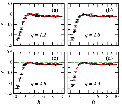
In practice, is obtained from the slope of the linear fit of versus . In Fig. 1, we show some representative examples of the scaling analysis for different values of and , and also for ensembles of different sizes , varying from to . The symbols are numerical data and the solid lines are the corresponding fitting curves.
In the chaotic region, for example when , the scaling of with is independent of the size of the ensemble, with all points and lines for a given coinciding and leading to . This is shown in Fig. 1 (a) for and it holds for all other values of that we studied, .
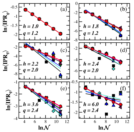
In contrast, when , the numerical points strongly depend on the number of samples used, as seen from Fig. 1 (b) to Fig. 1 (f). Notice that this dependence becomes more evident for the larger system sizes. In the particular cases of Figs. 1 (b)-(e), where , the fittings lead to larger slopes when the ensemble sizes are smaller. For these smaller ’s, the values of would get even larger if we would neglect the smallest system sizes when doing the fittings. These results illustrate the danger of reducing the number of samples as the system size increases.
We verify in Figs. 1 (b)-(f) that the convergence of our numerical points happens for ensembles with . Indeed the points for and are nearly indistinguishable, so in all of our subsequent studies, we use for all ’s. It may be, however, that for system sizes larger than the ones considered here, convergence would require even larger ensembles.
Self-averaging.– The fluctuations of the values of bring us to the discussion of self-averaging. A given quantity is self-averaging when its relative variance decreases as the system size increases [48, 49, 50, 51, 52, 53, 54, 55, 56]. This implies that in the thermodynamic limit, the result for a single sample agrees with the average over the whole ensemble of samples.
In quantum many-body systems, the eigenstates can spread over the many-body Hilbert space, which is exponentially large in , so we study the scaling of with [57, 46],
| (3) |
If , then is self-averaging and one can reduce the number of samples for the average as the system size increases. This cannot be done when , and it is even worse in the extreme scenario where and the relative fluctuations increase as the system size grows.
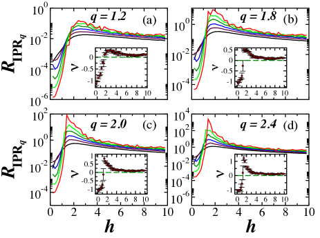
In the main panels of Fig. 2, we show the dependence of on the disorder strength for different values of and each line represents one system size. It is clear that deep in the chaotic region, the relative variance decreases as the system size grows, implying self-averaging of . This is also illustrated in the insets, where for , which is consistent with Fig. 1 (a), where the scaling of does not depend on the number of samples.
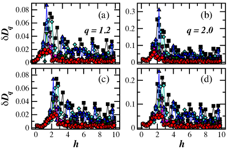
There is, however, a turning point at , where suddenly jumps above zero and grows significantly with system size. As seen in Figs. 2 (a)-(d), this is particularly bad in the region preceding the MBL phase, . For this range of disorder strength, as the insets indicate, and it reaches large values when [Figs. 2 (c)-(d)].
For , where the system should already be in the MBL phase, the relative variance continues to grow with system size, but is close to zero and the curves for and are not far from each other.
The results in Fig. 1 and Fig. 2 show that extra care needs to be taken when performing scaling analysis away from the chaotic region, not only due to finite-size effects, but also due to the lack of self-averaging. No matter how large the system size is, large numbers of samples are required and may even need to be increased as grows.
One can reduce the fluctuations of the generalized inverse participation ratios by using their logarithm, known as participation Rényi entropies. In fact, using a toy model, it was shown in [46] that in the MBL phase, grows with system size, while decreases with . However, for , even though we observe a reduction of the fluctuations, remains non-self-averaging and we still have [75]. We indeed verified that the plots shown in Fig. 1 remain similar if instead of , we use .
Multifractality and analytical expression for .– After taken the necessary precautions for performing the scaling analysis of the generalized inverse participation ratios, as discussed in Fig. 1, we now proceed with the study of how depends on and .
In Refs. [67, 68], an exact analytical expression was derived for the structure of the eigenstate at the center of the spectrum of the off-diagonal version of the Fibonacci model in the thermodynamic limit, leading to the generalized dimensions
| (4) |
where is the golden mean and is the maximum eigenvalue of the transfer matrix [67, 68]. For the Fibonacci model, denotes the ratio between its two hopping constants, which are arranged in a Fibonacci sequence.
In the case of our interacting spin model, we use Eq. (4) as an ansatz. Since in this case, the eigenstates are extended for , while Eq. (4) predicts a monotonic decrease of for , we compare our results with the expression for , where is the Heaviside step function. We find that this expression matches the numerical values of for the spin chain extremely well for disorder strengths in the vicinity of the critical value, .
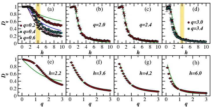
The inverse participation ratio, , is the most commonly used quantity in studies of localization, so we start by analyzing and as a function of the disorder strength. They are shown in Fig. 3 (b) and Fig. 3 (c), respectively. The numerical results agree very well with the analytical expression for for all ’s. However, for smaller ’s, the agreement is not as good, as illustrated in Fig. 3 (a), the same happening for larger ’s, as seen in Fig. 3 (d).
We cannot say whether the agreement of the curves for vs with for away from 2 would improve or get even worse if larger system sizes were considered. If it would improve, that would point to the existence of an extended phase of multifractal eigenstates before the MBL phase and described by the analytical expression of the Fibonacci lattice. Large-scale numerical studies [39, 41] indicate that if such a phase exists, it should appear for [41], and it may as well be a single point [39].
We stress, however, that the most relevant and less controversial information provided by Fig. 3 (a) and Fig. 3 (d) is that the numerical points for different values of ’s cross the curve of the analytical expression of at [shaded area in Fig. 3 (a) and Fig. 3 (d)]. This indicates that at least in the vicinity of (or right at) the critical point, the generalized dimensions of the disordered spin model is indeed extremely well described by Eq. (4).
The bottom panels of Fig. 3 give further support for this observation. There, we plot as a function of for different values of the disorder strength. For , as illustrated by Fig. 3 (e), there is no good agreement between the numerical points and . The same happens for , as seen in Fig. 3 (h), although the mismatch in this case is not as large. However, for , as shown in Fig. 3 (f) and Fig. 3 (g), the agreement is extremely good.
Conclusions.– Our analysis of the disordered spin-1/2 Heisenberg chain calls attention to the strong lack of self-averaging of the generalized inverse participation ratios for a range of disorder strengths that precedes the critical point of the MBL transition. This implies that in theoretical and experimental studies of this region, one should not decrease the number of samples as the system size increases. We notice also that the logarithm of the generalized inverse participation ratios can be used to reduce fluctuations, but it still does not lead to self-averaging in that region.
Our studies indicate a strong relationship between multifractality, , and the lack of self-averaging of the generalized inverse participation ratios, . Multifractality reflects the fragmentation of the Hilbert space [76], and this fragmentation, in turn, leads to the sample-to-sample fluctuations associated with the absence of self-averaging of . The latter should then hint at the existence of multifractal states.
The comparison between our numerical results for the generalized dimensions of the disordered spin chain and the analytical expression for derived for the off-diagonal version of the Fibonacci model shows remarkable agreement in the vicinity of the MBL transition. This connection is useful for theoretical efforts seeking to adequately describe the critical point and may serve as a reference for studies of transport behavior. It should also motivate additional numerical studies to verify whether the agreement holds in a finite region or only at a single critical point.
Acknowledgements.
LFS was supported by the NSF grant No. DMR-1936006. E.J.T.-H. is grateful to LNS-BUAP for their supercomputing facility.References
- Anderson [1958] P. W. Anderson, Absence of diffusion in certain random lattices, Phys. Rev. 109, 1492 (1958).
- Lee and Ramakrishnan [1985] P. A. Lee and T. V. Ramakrishnan, Disordered electronic systems, Rev. Mod. Phys. 57, 287 (1985).
- Lagendijk et al. [2009] A. Lagendijk, B. van Tiggelen, and D. S. Wiersma, Fifty years of Anderson localization, Phys. Today 62, 24 (2009).
- Fleishman and Anderson [1980] L. Fleishman and P. W. Anderson, Interactions and the Anderson transition, Phys. Rev. B 21, 2366 (1980).
- Altshuler et al. [1997] B. L. Altshuler, Y. Gefen, A. Kamenev, and L. S. Levitov, Quasiparticle lifetime in a finite system: A nonperturbative approach, Phys. Rev. Lett. 78, 2803 (1997).
- Santos et al. [2004] L. F. Santos, G. Rigolin, and C. O. Escobar, Entanglement versus chaos in disordered spin systems, Phys. Rev. A 69, 042304 (2004).
- Santos et al. [2005] L. F. Santos, M. I. Dykman, M. Shapiro, and F. M. Izrailev, Strong many-particle localization and quantum computing with perpetually coupled qubits, Phys. Rev. A 71, 012317 (2005).
- Gornyi et al. [2005] I. V. Gornyi, A. D. Mirlin, and D. G. Polyakov, Interacting electrons in disordered wires: Anderson localization and low- transport, Phys. Rev. Lett. 95, 206603 (2005).
- Basko et al. [2006] D. Basko, I. Aleiner, and B. Altshuler, Metal–insulator transition in a weakly interacting many-electron system with localized single-particle states, Ann. Phys. 321, 1126 (2006).
- Oganesyan and Huse [2007] V. Oganesyan and D. A. Huse, Localization of interacting fermions at high temperature, Phys. Rev. B 75, 155111 (2007).
- Dukesz et al. [2009] F. Dukesz, M. Zilbergerts, and L. F. Santos, Interplay between interaction and (un)correlated disorder in one-dimensional many-particle systems: delocalization and global entanglement, New J. Phys. 11, 043026 (2009).
- Nandkishore and Huse [2015] R. Nandkishore and D. Huse, Many-body localization and thermalization in quantum statistical mechanics, Annu. Rev. Condens. Matter Phys. 6, 15 (2015).
- Luitz and Lev [2017] D. Luitz and Y. B. Lev, The ergodic side of the many-body localization transition, Ann. Phys. (Berlin) 529, 1600350 (2017).
- Alet and Laflorencie [2018] F. Alet and N. Laflorencie, Many-body localization: An introduction and selected topics, C. R. Phys. 19, 498 (2018).
- Abanin et al. [2019a] D. A. Abanin, E. Altman, I. Bloch, and M. Serbyn, Colloquium: Many-body localization, thermalization, and entanglement, Rev. of Mod. Phys. 91, 021001 (2019a).
- Schreiber et al. [2015] M. Schreiber, S. S. Hodgman, P. Bordia, H. P. Lüschen, M. H. Fischer, R. Vosk, E. Altman, U. Schneider, and I. Bloch, Observation of many-body localization of interacting fermions in a quasirandom optical lattice, Science 349, 842 (2015).
- Kondov et al. [2015] S. Kondov, W. McGehee, W. Xu, and B. DeMarco, Disorder-induced localization in a strongly correlated atomic hubbard gas, Physical review letters 114, 083002 (2015).
- Smith et al. [2016] J. Smith, A. Lee, P. Richerme, B. Neyenhuis, P. W. Hess, P. Hauke, M. Heyl, D. A. Huse, and C. Monroe, Many-body localization in a quantum simulator with programmable random disorder, Nat. Phys. 12, 907 (2016).
- Bordia et al. [2016] P. Bordia, H. P. Lüschen, S. S. Hodgman, M. Schreiber, I. Bloch, and U. Schneider, Coupling identical one-dimensional many-body localized systems, Phys. Rev. Lett. 116, 140401 (2016).
- y. Choi et al. [2016] J. y. Choi, S. Hild, J. Zeiher, P. Schauss, A. Rubio-Abadal, T. Yefsah, V. Khemani, D. A. Huse, I. Bloch, and C. Gross, Exploring the many-body localization transition in two dimensions, Science 352, 1547 (2016).
- Bordia et al. [2017a] P. Bordia, H. Lüschen, U. Schneider, M. Knap, and I. Bloch, Periodically driving a many-body localized quantum system, Nat. Phys. 13, 460 (2017a).
- Bordia et al. [2017b] P. Bordia, H. Lüschen, S. Scherg, S. Gopalakrishnan, M. Knap, U. Schneider, and I. Bloch, Probing slow relaxation and many-body localization in two-dimensional quasiperiodic systems, Phys. Rev. X 7, 041047 (2017b).
- Lukin et al. [2019] A. Lukin, M. Rispoli, R. Schittko, M. E. Tai, A. M. Kaufman, S. Choi, V. Khemani, J. Léonard, and M. Greiner, Probing entanglement in a many-body–localized system, Science 364, 256 (2019).
- Kohlert et al. [2019] T. Kohlert, S. Scherg, X. Li, H. P. Lüschen, S. D. Sarma, I. Bloch, and M. Aidelsburger, Observation of many-body localization in a one-dimensional system with a single-particle mobility edge, Phys. Rev. Lett. 122, 170403 (2019).
- Rispoli et al. [2019] M. Rispoli, A. Lukin, R. Schittko, S. Kim, M. E. Tai, J. Léonard, and M. Greiner, Quantum critical behaviour at the many-body localization transition, Nature 573, 385 (2019).
- Zhu et al. [2020] D. Zhu, S. Johri, N. H. Nguyen, C. H. Alderete, K. A. Landsman, N. M. Linke, C. Monroe, and A. Y. Matsuura, Probing many-body localization on a noisy quantum computer (2020), arXiv:2006.12355.
- Luca and Scardicchio [2013] A. D. Luca and A. Scardicchio, Ergodicity breaking in a model showing many-body localization, Europhys. Lett. 101, 37003 (2013).
- Luitz et al. [2014] D. J. Luitz, F. Alet, and N. Laflorencie, Universal behavior beyond multifractality in quantum many-body systems, Phys. Rev. Lett. 112, 057203 (2014).
- Luitz et al. [2015] D. J. Luitz, N. Laflorencie, and F. Alet, Many-body localization edge in the random-field Heisenberg chain, Phys. Rev. B 91, 081103 (2015).
- Li et al. [2015] X. Li, S. Ganeshan, J. Pixley, and S. D. Sarma, Many-body localization and quantum nonergodicity in a model with a single-particle mobility edge, Phys. Rev. Lett. 115, 186601 (2015).
- Goold et al. [2015] J. Goold, C. Gogolin, S. R. Clark, J. Eisert, A. Scardicchio, and A. Silva, Total correlations of the diagonal ensemble herald the many-body localization transition, Phys. Rev. B 92, 180202 (2015).
- Torres-Herrera and Santos [2015] E. J. Torres-Herrera and L. F. Santos, Dynamics at the many-body localization transition, Phys. Rev. B 92, 014208 (2015).
- Li et al. [2016] X. Li, J. H. Pixley, D.-L. Deng, S. Ganeshan, and S. D. Sarma, Quantum nonergodicity and fermion localization in a system with a single-particle mobility edge, Phys. Rev. B 93, 184204 (2016).
- Serbyn and Moore [2016] M. Serbyn and J. E. Moore, Spectral statistics across the many-body localization transition, Phys. Rev. B 93, 041424 (2016).
- De Roeck et al. [2016] W. De Roeck, F. Huveneers, M. Müller, and M. Schiulaz, Absence of many-body mobility edges, Phys. Rev. B 93, 014203 (2016).
- De Roeck and Huveneers [2017] W. De Roeck and F. Huveneers, Stability and instability towards delocalization in many-body localization systems, Phys. Rev. B 95, 155129 (2017).
- Torres-Herrera and Santos [2017] E. J. Torres-Herrera and L. F. Santos, Extended nonergodic states in disordered many-body quantum systems, Ann. Phys. (Berlin) 529, 1600284 (2017).
- Serbyn et al. [2017] M. Serbyn, Z. Papić, and D. A. Abanin, Thouless energy and multifractality across the many-body localization transition, Phys. Rev. B 96, 104201 (2017).
- Macé et al. [2019] N. Macé, F. Alet, and N. Laflorencie, Multifractal scalings across the many-body localization transition, Phys. Rev. Lett. 123, 180601 (2019).
- Tarzia [2020] M. Tarzia, Many-body localization transition in Hilbert space, Phys. Rev. B 102, 014208 (2020).
- Luitz et al. [2020] D. J. Luitz, I. M. Khaymovich, and Y. B. Lev, Multifractality and its role in anomalous transport in the disordered XXZ spin-chain, SciPost Phys. Core 2, 6 (2020).
- Ghosh et al. [2020] S. Ghosh, J. Gidugu, and S. Mukerjee, Transport in the nonergodic extended phase of interacting quasiperiodic systems, Phys. Rev. B 102, 224203 (2020).
- [43] J. Suntajš, J. Bonča, T. Prosen, and L. Vidmar, Quantum chaos challenges many-body localization, arXiv:1905.06345.
- Abanin et al. [2019b] D. A. Abanin, J. H. Bardarson, G. D. Tomasi, S. Gopalakrishnan, V. Khemani, S. A. Parameswaran, F. Pollmann, A. C. Potter, M. Serbyn, and R. Vasseur, Distinguishing localization from chaos: challenges in finite-size systems (2019b), arXiv:1911.04501.
- Kiefer-Emmanouilidis et al. [2021] M. Kiefer-Emmanouilidis, R. Unanyan, M. Fleischhauer, and J. Sirker, Slow delocalization of particles in many-body localized phases, Phys. Rev. B 103, 024203 (2021).
- Torres-Herrera et al. [2020a] E. J. Torres-Herrera, G. De Tomasi, M. Schiulaz, F. Pérez-Bernal, and L. F. Santos, Self-averaging in many-body quantum systems out of equilibrium: Approach to the localized phase, Phys. Rev. B 102, 094310 (2020a).
- Tomasi et al. [2011] G. D. Tomasi, I. M. Khaymovich, F. Pollmann, and S. Warzel, Rare thermal bubbles at the many-body localization transition from the fock space point of view (2011), arXiv:2011.03048.
- Wiseman and Domany [1995] S. Wiseman and E. Domany, Lack of self-averaging in critical disordered systems, Phys. Rev. E 52, 3469 (1995).
- Aharony and Harris [1996] A. Aharony and A. B. Harris, Absence of self-averaging and universal fluctuations in random systems near critical points, Phys. Rev. Lett. 77, 3700 (1996).
- Wiseman and Domany [1998] S. Wiseman and E. Domany, finite-size scaling and lack of self-averaging in critical disordered systems, Phys. Rev. Lett. 81, 22 (1998).
- Castellani and Cavagna [2005] T. Castellani and A. Cavagna, Spin-glass theory for pedestrians, J. Stat. Mech. Th. Exp. 2005, P05012 (2005).
- Malakis and Fytas [2006] A. Malakis and N. G. Fytas, Lack of self-averaging of the specific heat in the three-dimensional random-field Ising model, Phys. Rev. E 73, 016109 (2006).
- Roy and Bhattacharjee [2006] S. Roy and S. M. Bhattacharjee, Is small-world network disordered?, Phys. Lett. A 352, 13 (2006).
- Monthus [2006] C. Monthus, Random Walks and Polymers in the Presence of Quenched Disorder, Lett. Math. Phys. 78, 207 (2006).
- Efrat and Schwartz [2014] A. Efrat and M. Schwartz, Lack of self-averaging in random systems - Liability or asset?, Phys. A Stat. Mech. Appl. 414, 137 (2014).
- Łobejko et al. [2018] M. Łobejko, J. Dajka, and J. Łuczka, Self-averaging of random quantum dynamics, Phys. Rev. A 98, 022111 (2018).
- Schiulaz et al. [2020] M. Schiulaz, E. J. Torres-Herrera, F. Pérez-Bernal, and L. F. Santos, Self-averaging in many-body quantum systems out of equilibrium: Chaotic systems, Phys. Rev. B 101, 174312 (2020).
- Torres-Herrera et al. [2020b] E. J. Torres-Herrera, I. Vallejo-Fabila, A. J. Martínez-Mendoza, and L. F. Santos, Self-averaging in many-body quantum systems out of equilibrium: Time dependence of distributions, Phys. Rev. E 102, 062126 (2020b).
- Vosk et al. [2015] R. Vosk, D. A. Huse, and E. Altman, Theory of the many-body localization transition in one-dimensional systems, Phys. Rev. X 5, 031032 (2015).
- Zhang et al. [2016] L. Zhang, B. Zhao, T. Devakul, and D. A. Huse, Many-body localization phase transition: A simplified strong-randomness approximate renormalization group, Phys. Rev. B 93, 224201 (2016).
- Dumitrescu et al. [2017] P. T. Dumitrescu, R. Vasseur, and A. C. Potter, Scaling theory of entanglement at the many-body localization transition, Phys. Rev. Lett. 119, 110604 (2017).
- Thiery et al. [2018] T. Thiery, F. m. c. Huveneers, M. Müller, and W. De Roeck, Many-body delocalization as a quantum avalanche, Phys. Rev. Lett. 121, 140601 (2018).
- Goremykina et al. [2019] A. Goremykina, R. Vasseur, and M. Serbyn, Analytically solvable renormalization group for the many-body localization transition, Phys. Rev. Lett. 122, 040601 (2019).
- Dumitrescu et al. [2019] P. T. Dumitrescu, A. Goremykina, S. A. Parameswaran, M. Serbyn, and R. Vasseur, Kosterlitz-thouless scaling at many-body localization phase transitions, Phys. Rev. B 99, 094205 (2019).
- Morningstar and Huse [2019] A. Morningstar and D. A. Huse, Renormalization-group study of the many-body localization transition in one dimension, Phys. Rev. B 99, 224205 (2019).
- Morningstar et al. [2020] A. Morningstar, D. A. Huse, and J. Z. Imbrie, Many-body localization near the critical point, Phys. Rev. B 102, 125134 (2020).
- Fujiwara et al. [1989] T. Fujiwara, M. Kohmoto, and T. Tokihiro, Multifractal wave functions on a Fibonacci lattice, Phys. Rev. B 40, 7413 (1989).
- Hiramoto and Kohmoto [1992] H. Hiramoto and M. Kohmoto, Electronic spectral and wavefunction properties of one-dimensional quasiperiodic systems: a scaling approach, Int. J. Mod. Phys. B 06, 281 (1992).
- Guhr et al. [1998] T. Guhr, A. Mueller-Gröeling, and H. A. Weidenmüller, Random matrix theories in quantum physics: Common concepts, Phys. Rep. 299, 189 (1998).
- Pal and Huse [2010] A. Pal and D. A. Huse, Many-body localization phase transition, Phys. Rev. B 82, 174411 (2010).
- Berkelbach and Reichman [2010] T. C. Berkelbach and D. R. Reichman, Conductivity of disordered quantum lattice models at infinite temperature: Many-body localization, Phys. Rev. B 81, 224429 (2010).
- Kjäll et al. [2014] J. A. Kjäll, J. H. Bardarson, and F. Pollmann, Many-body localization in a disordered quantum ising chain, Phys. Rev. Lett. 113, 107204 (2014).
- Devakul and Singh [2015] T. Devakul and R. R. Singh, Early breakdown of area-law entanglement at the many-body delocalization transition, Phys. Rev. Lett. 115, 187201 (2015).
- Doggen et al. [2018] E. V. H. Doggen, F. Schindler, K. S. Tikhonov, A. D. Mirlin, T. Neupert, D. G. Polyakov, and I. V. Gornyi, Many-body localization and delocalization in large quantum chains, Phys. Rev. B 98, 174202 (2018).
- [75] Supplemental material.
- Pietracaprina and Laflorencie [2019] F. Pietracaprina and N. Laflorencie, Hilbert space fragmentation and many-body localization (2019), arXiv:1906.05709 .
Supplemental Material:
Multifractality and self-averaging at the many-body localization transition
Andrei Solórzano,1 Lea F. Santos,2 and E. Jonathan Torres-Herrera3
1Tecnológico de Monterrey, Escuela de Ingeniería y Ciencias,
Ave. Eugenio Garza Sada 2501, Monterrey, N.L., Mexico, 64849.
2Department of Physics, Yeshiva University, New York, New York 10016, USA
3Instituto de Física, Benemérita Universidad Autónoma de Puebla, Apt. Postal J-48, Puebla, 72570, Mexico
In this supplemental material (SM), we show that the application of a logarithmic transformation to the generalized inverse participation ratios of the energy eigenstates reduces the size of the fluctuations, but is not enough to achieve self-averaging, specially around the critical point. This implies that reducing the numbers of statistical data to compute averages as the system size increases remains a problem also in this case.
We also present results for the errors involved in the computation of the generalized dimensions. We find that the errors obtained for the linear fit of versus and those for versus are very similar. They are larger in the vicinity of the critical point and get significantly larger for all values of as one decreases the size of the ensembles, while in the chaotic region, , we have that for all numbers of samples considered. This reinforces our claims that outside the chaotic region, we should not reduce the size of the ensembles as the system size increases, especially in the vicinity of the critical point.
I Logarithm of the generalized participation ratios
An alternative approach to compute the generalized dimensions consists in using the logarithm of the generalized participation ratios,
| (S1) |
which corresponds to the so-called participation Rényi entropies. In this case, instead of doing the linear fit of versus , as in the main text, we study
| (S2) |
That is, instead of computing the logarithm of the averaged generalized inverse participation ratios, which is an arithmetic mean, we now compute the average of the logarithm of the generalized participation ratios, which is a geometric mean. The logarithmic transformation is commonly applied to reduce the fluctuations of a set of data and it has a significant effect on the tails of the distributions.
In Fig. S1, we show for . Comparing it with the insets of the Fig. 2 in the main text, we see two main differences. One is that in the localized phase, becomes self-averaging, in agreement to what was discussed in Ref. [42]. The other difference is that the values of around the critical point become much smaller, but it is still not negative, so the lack of self-averaging persists.
II Errors
As show in Fig. S2, there is no significant difference between the error obtained by extracting the generalized dimensions from the scaling of with [ in Figs. S2 (a)-(b)] and that from the scaling of with [ in Figs. S2 (c)-(d)]. The results in all four panels are very similar. In the chaotic region, , is close to zero for all ensemble sizes considered. The errors increase monotonically for , but remain almost independent of the number of samples. It is in the vicinity of the critical point, , that the errors become clearly larger as the number of samples gets decreased. For , the errors still depend on the number of samples, but they are smaller that in the preceding region, specially for the ensembles with samples for which a sudden drop is seen at .