Uncovering the High Scale Higgs Singlet Model

Abstract

The scalar singlet model extends the Standard Model with the addition of a new gauge singlet scalar. We re-examine the limits on the new scalar from oblique parameter fits and from a global fit to precision electroweak observables and present analytic expressions for our results. For the case when the new scalar is much heavier than the weak scale, we map the model onto the dimension-six Standard Model effective field theory (SMEFT) and review the allowed parameter space from unitarity considerations and from the requirement that the electroweak minimum be stable. A global fit to precision electroweak data, along with LHC observables, is used to constrain the parameters of the high scale singlet model and we determine the numerical effects of performing the matching at both tree level and 1-loop.

I Introduction

The Higgs singlet model Bowen:2007ia ; O'Connell:2006wi ; Dawson:2015haa ; Muhlleitner:2020wwk ; Robens:2015gla ; Costa:2015llh ; Chen:2014ask has been extensively studied as a simple extension of the Standard Model (SM) containing only one new particle. Depending on the potential parameters, the model can lead to a first order electroweak phase transition Huber:2006wf ; Profumo:2007wc ; Espinosa:2011ax ; Barger:2011vm ; Profumo:2014opa ; Curtin:2014jma ; Kotwal:2016tex ; Huang:2017jws ; Chen:2017qcz ; Kurup:2017dzf ; Li:2019tfd , making it highly motivated in addressing the problem of baryogenesis. It can also arise as the limiting case of many interesting models addressing the hierarchy problem Craig:2013xia ; Curtin:2015bka or even dark matter Silveira:1985rk ; McDonald:1993ex ; Burgess:2000yq ; Menon:2004wv ; He:2008qm ; Gonderinger:2009jp ; Mambrini:2011ik . When the mass of the new scalar becomes much larger than the weak scale, the theory can be mapped onto an effective field theory. The utility and simplicity of the model thus makes it an ideal candidate for exploring the limits of an effective field theory framework in reproducing the features of the underlying UV models Dawson:2020oco ; Brehmer:2015rna ; Henning:2014gca ; Henning:2014wua ; Gorbahn:2015gxa ; Ellis:2018gqa ; Ellis:2020unq ; Anisha:2020ggj .

In the full UV complete singlet model, restrictions on the parameters can be found from fits to precision electroweak observables as well as LHC data. These limits can then be compared with limits found in the context of a low energy effective field theory. We consider an effective field theory in which the SM Higgs doublet is constrained to be an $SU(2)$ doublet, the Standard Model effective field theory (SMEFT). At tree level, the singlet model generates only two SMEFT coefficients when matched at the UV scale Henning:2014wua ; Egana-Ugrinovic:2015vgy . The aim of this work is to examine to what extent the extraction of SMEFT coefficients from global fits at the weak scale gives information on the parameters of the UV complete singlet model Ellis:2018gqa ; Ellis:2020unq ; Dawson:2020oco ; Bakshi:2020eyg ; Kribs:2017znd ; Falkowski:2015iwa ; Gorbahn:2015gxa . The focus is on understanding the numerical importance of various choices made when performing the low energy fits and to this end, we implement both tree and 1-loop matching Jiang:2018pbd ; Haisch:2020ahr ; Cohen:2020fcu at the UV scale. We find that the effects of the 1-loop matching are typically rather small. Effects of ${\cal{O}}(10\%)$ can be obtained only for rather large values of certain dimensionless parameters in the Lagrangian.

Section II contains a recap of the model and restrictions on the model parameters from unitarity and the minimization of the potential. Analytic results for electroweak precision observables in the singlet model are found in Section III along with a comparison between a global fit to electroweak precision observables (EWPOs) and a fit to the oblique parameters, and restrictions from unitarity and the minimization of the potential are in Section IV. The SMEFT matching with the singlet model at both tree and loop level is studied in Section V and a global fit to electroweak precision observables, Higgs, and di-boson data is presented. Section VI has some conclusions.

II Basics

The singlet model we consider contains the SM Higgs doublet, $\Phi$, and a scalar gauge singlet, $S$. The most general scalar potential is,

$$V(\Phi,S)= -\mu_{H}^{2}\Phi^{\dagger}\Phi+\lambda_{H}(\Phi^{\dagger}\Phi)^{2}$$

$$+\frac{m_{\xi}}{2}\Phi^{\dagger}\Phi S+\frac{\kappa}{2}\Phi^{\dagger}\Phi S^{2}$$

$$+t_{S}S+\frac{M^{2}}{2}S^{2}+\frac{m_{\zeta}}{3}S^{3}+\frac{\lambda_{S}}{4}S^{4}\,.$$ (1)

The parameters can be redefined such that $\langle{S}\rangle\equiv x=0$. After spontaneous symmetry breaking, the 2 neutral scalars, $\Phi_{0}$ and ${S}$, mix to form the physical scalars, $h$ and $H$,

$$h = \cos\theta\,{\Phi_{0}}+\sin\theta\,{S}$$

$$H = -\sin\theta\,{\Phi_{0}}+\cos\theta\,{S}\,,$$ (2)

with the physical masses, $m_{h}=125.1\,\textrm{GeV}$ and $M_{H}$. The parameters of the model can be taken as,

$$m_{h},\quad M_{H},\quad v=246\,\textrm{GeV},\quad\sin\theta,\quad x=0,\quad\kappa,\quad m_{\zeta},\quad\lambda_{S}\,.$$ (3)

The other parameters of the Lagrangian are determined in the singlet model by:

$$m_{\xi} = \frac{m_{h}^{2}-M_{H}^{2}}{v}\sin 2\theta\,,$$

$$M^{2} = m_{h}^{2}\sin^{2}\theta+M_{H}^{2}\cos^{2}\theta-\frac{\kappa}{2}v^{2}\,,$$

$$\lambda_{H} = \frac{m_{h}^{2}\cos^{2}\theta+M_{H}^{2}\sin^{2}\theta}{2v^{2}}\,.$$ (4)

The $Z_{2}$ symmetric case has $m_{\zeta}=t_{S}=m_{\xi}=0$ and $x\neq 0$.

The couplings of $h$ to SM fermions and gauge bosons are suppressed relative to the SM Higgs couplings by a factor of $\cos\theta$, while the $H$ couplings are suppressed by $\sin\theta$. We can thus immediately find a trivial limit on $\cos\theta$ from Higgs production to SM particles $X$, (assuming no decays to invisible particles),

$$\cos^{2}\theta = \mu\equiv\frac{\sigma\cdot\textrm{BR}}{(\sigma\cdot\textrm{BR})_{\textrm{SM}}}$$ (5)

Naively combining the combined ATLAS results with $80\,\textrm{fb}^{-1}$ Aad:2019mbh and the CMS combined limits with $139\,\textrm{fb}^{-1}$ CMS:2020gsy ,

$$\mu[\textrm{ATLAS}]=1.11^{+.09}_{-.08},\qquad\mu[\textrm{CMS}]=1.02^{+.07}_{-.06}$$ (6)

we find at $95\%$ C.L.,

$$|\sin\theta\,|<0.2\quad\text{for}\quad m_{h}<2M_{H}\,.$$ (7)

For $m_{h}>2M_{H}$, the naive limit of Eq. (7) does not apply because the $h$ decays to $HH$ must be included and this branching ratio is sensitive to the other parameters of the scalar potential. Limits on the singlet model from resonant double Higgs production are beginning to be competitive with those from single Higgs production for $M_{H}\lesssim 700\,\textrm{GeV}$ Aad:2019uzh , although our primary focus here will be on $M_{H}\sim(1-2)\,\textrm{TeV}$.

III Restrictions on Model Parameters

The parameters of the singlet model can be limited by a fit to the $Z$- and $W$-pole observables (we term this the EWPO fit):

$$M_{W},~{}~{}\Gamma_{W},~{}~{}\Gamma_{Z},~{}~{}\sigma_{h},~{}~{}R_{b},~{}~{}R_{c},~{}~{}R_{l},~{}~{}A_{FB,b},~{}~{}A_{FB,c},~{}~{}A_{FB,l},~{}~{}A_{b},~{}~{}A_{c},~{}~{}A_{l}\,.$$ (8)

The SM results for these observables are well known Hollik:1988ii ; Freitas:2014hra . In a previous study, Ref. Dawson:2019clf , we computed the limits on the coefficients of an effective field theory that result from a fit to the observables of Eq. (8) computed to NLO in both QCD and electroweak interactions, and we apply an identical calculational framework here. The observables and SM theory numbers used in the current study can be found in in Table III of Ref. Dawson:2019clf . We take as our input parameters: $G_{\mu}=1.1663787(6)\times 10^{-5}\,\textrm{GeV}^{-2}$, $M_{Z}=91.1876\pm.0021\,\textrm{GeV}$, $1/\alpha={137.035999139(31)}$, $\Delta\alpha_{\rm had}^{(5)}=0.02764\pm 0.00009$, $\alpha_{s}(M_{Z})=0.1181\pm 0.0011$,   $m_{h}=125.10\pm 0.14\,\textrm{GeV}$,  $m_{b}=4.18\,\textrm{GeV}$ and $M_{t}=172.9\pm 0.5\,\textrm{GeV}$ .

The one loop relation between the Fermi constant $G_{\mu}$ and the vacuum expectation value $v$ is, as usual,

$$G_{\mu}=\frac{1}{\sqrt{2}v^{2}}(1+\Delta r)$$ (9)

where,

$$\Delta r=\Delta r_{\textrm{SM}}+\Delta r_{\textrm{singlet}}.$$

In computing $\Delta r$, we use ${\hat{M}}_{W}^{2}\equiv(M_{Z}^{2}/2)\bigg{(}1+\sqrt{1-\frac{\sqrt{8}\pi\alpha}{G_{\mu}M_{Z}^{2}}}\bigg{)}$ calculated from our inputs. For simplicity, we define $h\equiv m_{h}^{2}$, $H\equiv M_{H}^{2}$, $z\equiv M_{Z}^{2}$ and $w\equiv{\hat{M}}_{W}^{2}$ and obtain the simple form,

$$\Delta r_{\textrm{singlet}} =\Delta r_{\textrm{singlet}}(h,H)-\Delta r_{\textrm{singlet}}(H,h)$$

$$\Delta r_{\textrm{singlet}}(h,H) ={\sqrt{2}\sin^{2}\theta G_{\mu}\over 16\pi^{2}}\biggl{\{}-{h\over 2}+{3wA_{0}(h)\over(h-w)}+{3whA_{0}(w)\over(H-w)(h-w)}\biggr{\}}\,.$$ (10)

We find the one-loop prediction for $M_{W}$ in the singlet model,

$$M_{W} = M_{W}^{\textrm{SM}}+F_{W}(h,H)-F_{W}(H,h)$$

$$F_{W}(h,H) = {\alpha\sin^{2}\theta\over 8\pi M_{W}}\biggl{\{}{hz\over 24(2w-z)}+{A_{0}(h)\over 12(h-w)w(2w-z)}\biggl{(}hw(w-4z)+12w^{2}z+h^{2}(z-w)\biggr{)}$$ (11)

$$+{hzA_{0}(w)\over 12(h-w)w(H-w)(z-w)(2w-z)}\biggl{(}(2w-z)\biggl{[}hH-w(h+H)\biggr{]}+w^{2}(8z-7w)\biggr{)}$$

$$+{hwA_{0}(z)\over 12(z-w)(z-2w)}-{zB_{0}(w,h,w)\over 12w(w-z)}\biggl{(}h^{2}-4hw+12w^{2}\biggr{)}$$

$$+{wB_{0}(z,h,z)\over 12(z-2w)(z-w)}\biggl{(}h^{2}-4hz+12z^{2}\biggr{)}\biggr{\}}\,.$$

This is in agreement with Ref. Lopez-Val:2014jva . For a massless $b$ quark, the total $W$ decay width is,

$$\Gamma_{W}= ~{}~{}\Gamma_{W}^{\textrm{SM}}+G_{W}(h,H)-G_{W}(H,h)$$

$$G_{W}(h,H)= -{3\sqrt{w}G_{F}^{2}\sin^{2}\theta\over 32\pi^{3}}\biggl{\{}{wh(-hH-8w^{2}+4wh+4wH)\over 2(h-4w)(H-4w)}$$

$$-{A_{0}(h)\over h(h-4w)(h-w)}\biggl{(}h^{4}-7h^{3}w+21h^{2}w^{2}-32hw^{3}+8w^{4}\biggr{)}$$

$$+{hA_{0}(w)\over(h-4w)(h-w)(H-w)(H-4w)}\biggl{(}4w^{2}(H^{2}+h^{2})-5whH(H+h)$$

$$+h^{2}H^{2}-4w^{3}(H+h)+18w^{2}hH-36w^{4}\biggr{)}$$

$$+{B_{0}(w,h,w)\over(h-4w)}\biggl{(}h^{3}-7h^{2}w+20hw^{2}-28w^{3}\biggr{)}\biggr{\}}\,.$$ (12)

Analytic expressions for the remaining observables of Eq. (8) are given in the supplemental material attached to this note.

The finite $b$ mass contribution to $Z$ decays to bottom pairs is sensitive to the Higgs-$b$ Yukawa coupling and generates non-oblique contributions. We compute $R_{l},R_{b},R_{c}$ and $\Gamma_{Z}$ for $m_{b}\neq 0$ and find that the numerical effect is less than $\sim 2\%$ for $M_{H}>20\,\textrm{GeV}$, rising to $\sim 5\%$ for $M_{H}\sim 10\,\textrm{GeV}$, justifying the neglect of $b$ mass effects in our fits.

We perform a fit, including correlations, to the observables of Eq. (8) to determine the maximum allowed value of $\sin\theta$ for a given value of $M_{H}$ including all one-loop contributions. It is of interest to compare the complete EWPO fit with the results using the oblique parameters only. Using the results of Dawson:2009yx ; Englert:2020gcp , we find that the differences between the Peskin-Takeuchi Peskin:1991sw variables in the Higgs singlet model and the SM take the form,

$$\Delta S =\frac{\sin^{2}\theta}{12\pi}(\mathcal{G}(H,z)-\mathcal{G}(h,z))$$ (13)

$$\Delta T =\frac{3\sin^{2}\theta}{16\pi s_{W}^{2}c_{W}^{2}}(\mathcal{K}(H)-\mathcal{K}(h))$$ (14)

$$\Delta S+\Delta U =\frac{\sin^{2}\theta}{12\pi c_{W}^{2}}(\mathcal{G}(H,w)-\mathcal{G}(h,w)),$$ (15)

where $s_{W}^{2}=1-c_{W}^{2}=1-w/z$ is $\sin^{2}\theta_{W}$ of the electroweak mixing angle and we define,

$$\mathcal{K}(h) =h(\frac{(z-w)}{(h-w)(h-z)}A_{0}(h)+\frac{A_{0}(w)}{(h-w)}-\frac{A_{0}(z)}{(h-z)})$$ (16)

$$\mathcal{G}(h,z) =\frac{h}{2}+\mathcal{F}(h,z)(A_{0}(h)-A_{0}(z)-(h-z)B_{0}(z,h,z))$$ (17)

$$\mathcal{F}(h,z) =\frac{h^{2}-4hz+12z^{2}}{z(h-z)}\,.$$ (18)

We fit to the values in Zyla:2020zbs ,

$$\Delta S =-0.01\pm 0.10$$

$$\Delta T =0.02\pm 0.12$$

$$\Delta U =0.02\pm 0.11\,$$ (19)

with the correlation matrix,

$$\rho=\left(\begin{array}[]{c c c}1.&0.92&-0.80\\ 0.92&1.&-0.93\\ -0.80&-0.93&1.\end{array}\right)\,.$$ (20)

In Fig. 1 we report the results corresponding to different sets of observables:

• Only $M_{W}$

• The $Z$ pole observables alone

• Oblique parameters only

• EWPOs given in Eq. (8).

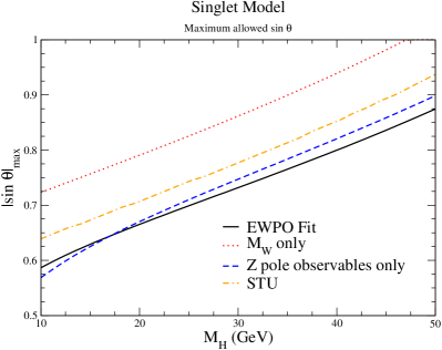
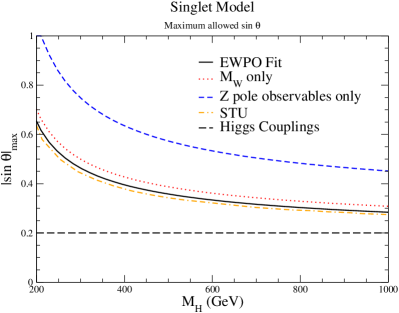
Figure 1: Maximum allowed $\sin\theta$ in the Higgs singlet model at $95\%$ confidence level based on fits to electroweak precision observables (EWPO), the $W$ mass measurement only, the $Z$ pole observables only, and to the $STU$ parameters as described in the text. A naive limit from the Higgs coupling measurements is shown on the RHS for comparison.

The results for the fit to $M_{W}$ alone are in agreement with those of Ref. Ilnicka:2018def and are a good approximation to the complete EWPO fit. The EWPO fit limits are in agreement with Ref. Falkowski:2015iwa after adjusting for the different input parameters. It is interesting that the current limits from Higgs couplings give better bounds for all $M_{H}\lesssim 1\,\textrm{TeV}$ as given in Eq. (7). The limits obtained from oblique parameters are in approximate agreement with those from the EWPO fit for a heavier second Higgs boson, although slightly different data sets and approximations were used in the numbers we fit to. For the case where the second Higgs is light, $M_{H}<m_{h}$, the limits obtained from the oblique parameters are not a good approximation of the complete EWPO fit.

IV Theoretical Constraints

In Section V, we will match the singlet model with a very heavy $H$ to the SMEFT. Before we do so, we consider the theoretical restrictions on the singlet model parameters that are relevant for the matching.

IV.1 Vacuum Structure of the Potential

The first set of theoretical constraints on the singlet model come from requiring a suitable vacuum structure of the potential Espinosa:2011ax ; Chen:2014ask ; Robens:2015gla ; Robens:2016xkb . Demanding that the potential is stable at large field values leads to the requirement $\lambda_{H},\lambda_{S}>0$, and $\kappa\geq-2\sqrt{\lambda_{H}\lambda_{S}}$ Chen:2014ask , where $\lambda_{H}$ is determined by Eq. (4). Additional bounds result from requiring that the electroweak minimum be the global minimum of the potential. Following Chen:2014ask , we compute these bounds by finding all the extrema of the potential expanded around the electroweak vev as a function of $(v,x)$, and then checking whether or not the value of the potential at $(v=246\,\textrm{GeV},x=0)$ is the global minimum.

The extrema of the potential can be divided into two classes: extrema where $v\neq 0$, and those where $v=0$. In the former case, the new extrema are denoted $(v_{\pm},x_{\pm})$ as in ref. Chen:2014ask , and tend to bound lower values of $\kappa$. In the latter case, the extrema are denoted by $(0,x^{0}_{\pm})$, and these tend to limit both large values of $\kappa$ as well as large values of $m_{\zeta}$. An example of the vacuum structure is shown in Fig. 2, where we illustrate the regions excluded by the emergence of different global minima as well as the condition from vacuum stability. Fig. 3 illustrates how these bounds change as a function of the physical parameters. In particular, we see that for larger masses, $M$, the bounds on $m_{\zeta}/M$ from the $v=0$ minima become constant as a function of $\kappa$, depending only on $\lambda_{S}$. It is interesting that quite large values of $\kappa$ are allowed in all scenarios. The upper bound on $m_{\zeta}/M$ never exceeds ${\cal{O}}(2-3)$.

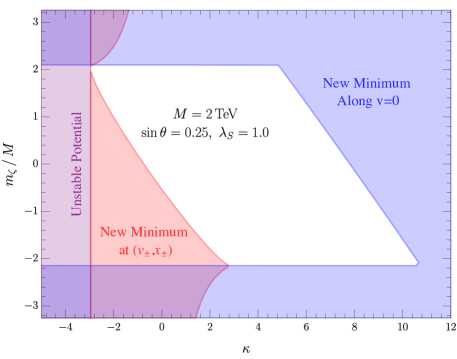
Figure 2: Demonstration of the bounds from the appearance of other global minima in the $\kappa$ vs. $m_{\zeta}/M$ plane for $M=2\,\textrm{TeV}$, $\sin\theta=0.25$, and $\lambda_{S}=1.0$ in the singlet model.

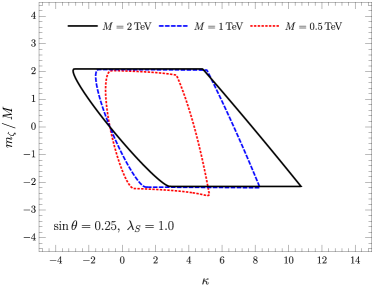
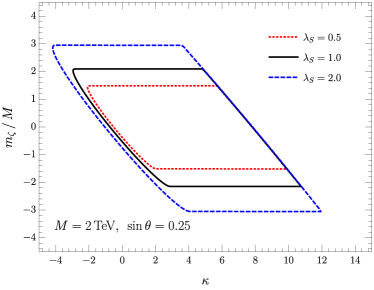
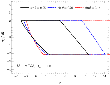
Figure 3: Regions in the singlet model where the electroweak minimum is the global minimum of the potential as a function of $\kappa$ and $m_{\zeta}/M$, varying the other physical parameters.

IV.2 Unitarity

The next set of theoretical constraints come from the requirements of tree-level perturbative unitarity Lee:1977yc ; Lee:1977eg ; Dawson:2017vgm ; Robens:2015gla . The simplest constraints come from $hh\to hh$ and $HH\to HH$ scattering, where the spin-$0$ partial waves in the high energy limit are

$$a_{0}(hh\to hh)\Big{|}_{s\gg m_{h}^{2}} =-\frac{3}{16\pi}\left(\lambda_{H}\cos^{4}{\theta}+\kappa\sin^{2}{\theta}\cos^{2}{\theta}+\lambda_{S}\sin^{4}{\theta}\right)$$ (21)

$$a_{0}(HH\to HH)\Big{|}_{s\gg m_{H}^{2}} =-\frac{3}{16\pi}\left(\lambda_{S}\cos^{4}{\theta}+\kappa\sin^{2}{\theta}\cos^{2}{\theta}+\lambda_{H}\sin^{4}{\theta}\right)$$ (22)

For $\sin\theta\ll 1$, requiring $|a_{0}|<1/2$ sets the bounds $\lambda_{S},\lambda_{H}\lesssim 8\pi/3$. This bound on $\lambda_{H}$ indirectly bounds $M_{H}$ as a function of $\sin\theta$:

$$M_{H}^{2}\,\sin^{2}\theta \lesssim \frac{16\pi}{3}v^{2}-m_{h}^{2}\,\cos^{2}\theta$$

$$M_{H} \lesssim 7\,\textrm{TeV}\quad{\rm{for}}\cos\theta=0.99\,.$$ (23)

The similar bound from $hH\to hH$ scattering only restricts $|\kappa|\lesssim 8\pi$.

V One-loop Matching of the Singlet Model to SMEFT

V.1 One-loop Matching

When the mass of the heavy scalar is much larger than the weak scale and any relevant energy scales, the singlet model can be modeled by an effective field theory,

$$\mathcal{L}_{\textrm{singlet}}~{}\xrightarrow[M_{H}\to\infty]{}~{}\mathcal{L}_{\textrm{SM}}+\sum_{i}\frac{C_{i}(M)}{M^{2}}\mathcal{O}_{i}^{(6)}+\dots$$ (24)

with coefficients matched to the singlet model at the high scale, $M$. We retain only the dimension-6 operators, $\mathcal{O}_{i}^{(6)}$ ,and use the Warsaw basis Buchmuller:1985jz with the notation of Ref. Dedes:2017zog .

The global fits of Ref. Dawson:2020oco were performed using tree level matching at the scale $M$. It is of interest to implement the one-loop matching for the case of the singlet model and examine the numerical impacts. The coefficients at the matching scale, $M$, generically take the form,

$$C_{i}(M)=c_{i}(M)+\frac{d_{i}(M)}{16\pi^{2}}\,,$$ (25)

where $c_{i}(M)$ is the tree level result and $d_{i}(M)/(16\pi^{2})$ is the one-loop contribution at the matching scale. When the renormalization group evolution to the low scale $\mu_{R}$ is included,

$$C_{i}(\mu_{R})=c_{i}(M)+{d_{i}(M)\over 16\pi^{2}}+{\gamma_{ij}\over 32\pi^{2}}c_{ij}(M)\log\biggl{(}{\mu_{R}^{2}\over M^{2}}\biggr{)}\,.$$ (26)

In the case of the singlet model only two coefficients are generated at tree level Egana-Ugrinovic:2015vgy ; Henning:2014wua ; deBlas:2017xtg ; Dawson:2017vgm ,

$$c_{H\square} = -{m_{\xi}^{2}\over 8M^{2}}$$ (27)

$$c_{H} = {m_{\xi}^{2}\over 8M^{2}}\biggl{(}{m_{\xi}m_{\zeta}\over 3M^{2}}-\kappa\biggr{)}\,,$$ (28)

with all other $c_{i}(M)=0$. However, there are many coefficients generated at one-loop at the matching scale, $M$ Jiang:2018pbd ; Cohen:2020fcu ; Haisch:2020ahr . The majority of these coefficients are proportional to the tree level coefficient, $c_{H\square}$. We use the shorthand $C_{Hu}\rightarrow C_{Hu},C_{Hc},C_{Ht}$, etc., and take $y_{u}=y_{c}=0,~{}y_{t}=M_{t}\sqrt{2}/v$ (similarly we set all other $y_{i}=0$) and we further assume that $C_{Hq}^{(1)},~{}C_{Hq}^{(3)},~{}C_{Hl}^{(1)}$, and $C_{Hl}^{(3)}$ are flavor diagonal and use an analogous shorthand. For convenience, we list the results of Ref. Jiang:2018pbd in our notation:

$$d_{HD} = {31g^{\prime~{}2}\over 9}c_{H\square}$$

$$d_{HW} = -{g^{2}\over 6}c_{H\square}$$

$$d_{HB} = -{g^{\prime~{}2}\over 6}c_{H\square}$$

$$d_{HWB} = -{gg^{\prime}\over 3}c_{H\square}$$

$$d_{Hu} = {1\over 108}(34g^{\prime~{}2}-135y_{u}^{2})c_{H\square}$$

$$d_{Hd} = {1\over 3}d_{He}={2\over 3}d_{Hl}^{(1)}=-{17g^{\prime~{}2}\over 108}c_{H\square}$$

$$d_{Hq}^{(1)} = {1\over 216}(17g^{\prime~{}2}+135y_{u}^{2})c_{H\square}$$

$$d_{Hq}^{(3)} = {1\over 72}\biggl{[}17g^{~{}2}-45y_{u}^{2}\biggr{]}c_{H\square}$$

$$d_{Hl}^{(3)} = {17g^{2}\over 72}c_{H\square}$$

$$d_{2y} = -{1\over 3}c_{H\square}\,.$$ (29)

The one-loop contribution $d_{tH}$ can be written in terms of $c_{H\square}$ and $C_{H}$ and is,

$$d_{tH}=y_{t}\bigg{[}-{1\over 18}(45y_{t}^{2}-31g^{2})c_{H\square}+{3\over 2}c_{H}-{29\over 3}\lambda\,c_{H\square}\bigg{]}\,,$$ (30)

where in the SMEFT the physical Higgs mass is determined in terms of the potential parameters to ${\cal{O}}(v^{2}/M^{2})$ by Dedes:2017zog ,

$${m_{h}^{2}\over 2v^{2}} = \lambda_{H}\biggl{(}1+{2v^{2}\over M^{2}}c_{H\square}\biggr{)}-{3\over 2}{v^{2}\over M^{2}}c_{H}$$ (31)

and we define,

$$\lambda \equiv {2\lambda_{H}}\biggl{(}1+{2v^{2}\over M^{2}}c_{H\square}\biggr{)}$$

$$\lambda = \frac{m_{h}^{2}}{v^{2}}+3\frac{v^{2}}{M^{2}}c_{H}+\mathcal{O}\bigg{(}\frac{v^{4}}{M^{4}}\bigg{)}\,,$$ (32)

where we note that Ref. Jiang:2018pbd absorbs the factor of $c_{H\square}$ into the definition of $\lambda$ used in the matching conditions, along with a relative factor of $2$ in the definition of the quartic terms in the potential. Eq. (31) represents the dimension-6 SMEFT limit of Eq. (4) for the relationship between the parameters of the potential and $m_{h}$.

Finally, the coefficients generated at tree level also receive one-loop corrections,

$$d_{H\square} =-\frac{9}{2}\lambda c_{H\square}+{31\over 36}(3g^{2}+g^{\prime~{}2})c_{H\square}+{3\over 2}c_{H}+\delta d_{H\square}+\delta d_{H\square}^{shift}$$

$$d_{H} =\lambda\biggl{[}\biggl{(}{62g^{2}-336\lambda\over 9}\biggr{)}c_{H\square}+6c_{H}\biggr{]}+\delta d_{H}+\delta d_{H}^{shift}\,.$$ (33)

where,

$$\delta d_{H}= -\frac{\kappa^{3}}{12}+\frac{m_{\xi}}{4M^{2}}\bigg{(}m_{\xi}\big{(}9\lambda^{2}-12\kappa\lambda+\frac{11}{2}\kappa^{2}-3\kappa\lambda_{S}\big{)}-\kappa^{2}m_{\zeta}\bigg{)}$$

$$+\frac{m_{\xi}^{2}}{6M^{4}}\bigg{(}\frac{m_{\xi}^{2}}{16}\big{(}39\kappa-18\lambda_{S}-36\lambda\big{)}+m_{\xi}m_{\zeta}\big{(}9\lambda-\frac{15}{2}\kappa+3\lambda_{S}\big{)}+3\kappa m_{\zeta}^{2}\bigg{)}$$

$$+\frac{m_{\xi}^{3}}{12M^{6}}\bigg{(}-\frac{1}{8}m_{\xi}^{3}-\frac{9}{8}m_{\xi}^{2}m_{\zeta}+3m_{\xi}m_{\zeta}^{2}-2m_{\zeta}^{3}\bigg{)}\,,$$ (34)

$$\delta d_{H\square}= -\frac{\kappa^{2}}{24}+\frac{m_{\xi}}{12M^{2}}\bigg{(}\frac{m_{\xi}}{2}\big{(}17\kappa-\frac{27}{2}\lambda-18\lambda_{S}\big{)}-5\kappa m_{\zeta}\bigg{)}$$

$$+\frac{m_{\xi}^{2}}{24M^{4}}\bigg{(}\frac{13}{8}m_{\xi}^{2}-8m_{\xi}m_{\zeta}+11m_{\zeta}^{2}\bigg{)}\,.$$ (35)

The terms of Eqs. (34) and (35) can be written in terms of $c_{H},c_{H\square}$ along with $m_{\zeta},\lambda_{S}$ and $\kappa$, ($m_{\xi}$ can be written in terms of these parameters). The one-loop shift terms from canonically normalizing the Higgs kinetic energy are,

$$\delta d_{H}^{shift} = 3c_{H\square}c_{H}\,,$$

$$\delta d_{H\square}^{shift} = 2(c_{H\square})^{2}\,.$$ (36)

The one-loop shift terms are ${\cal{O}}({v^{4}/M^{4}})$ and can be neglected, since we consistently work to linear order in the coefficient functions.

After performing the one-loop matching at $M$, the renormalization group is used to evolve the coefficients to $M_{Z}$, where the resulting coefficients can be compared with data. The complete set of one-loop anomalous dimension matrices can be found in Refs. Jenkins:2013zja ; Jenkins:2013wua ; Alonso:2013hga . The inclusion of the one-loop matching makes a relatively minor difference in the evolution of $C_{H}$ and $C_{H\square}$, as seen in Fig. 4 where we evolve from $2\,\textrm{TeV}$ (note that $M_{H}$ is related to $M$ by Eq. (4)). In Fig. 5, we show the effect of the one-loop matching on the evolution of $C_{HD}$. In this case, since $C_{HD}$ is zero at tree level, the contributions from the $1-$loop matching and the renormalization group running are of the same order of magnitude and the effects are more significant. In Fig. 6 we show the relative size of the $1-$loop matching compared to the tree level matching as the matching scale $M$ is increased and the overall effects are between $10-30\%$. The size of the effects for $C_{H\square}$ and $C_{H}$ increase dramatically as the matching scale rises over a few TeV. This is due to the logarithmic running becoming large and in the case of $C_{H}$, the 1-loop matching terms become of the same order as the tree level terms, implying that the perturbative expansion is no longer valid.

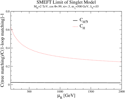
Figure 4: Renormalization group evolution of coefficient functions from the matching scale, $M$, to $\mu_{R}$ when the matching is done at tree level and at one-loop for coefficients that are generated at tree level. The coefficients are evaluated as a function of the running scale, $\mu_{R}$.

Figure 5: Renormalization group evolution of the coefficient function from the matching scale, $M$, to $\mu_{R}$ for $C_{HD}$, which is generated only by the renormalization group running in the singlet model. $C_{HD}$ is evaluated as a function of the running scale, $\mu_{R}$.

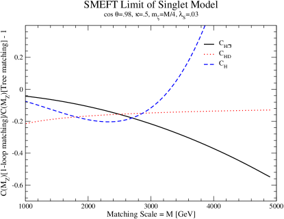
Figure 6: Shift in the coefficient functions at $M_{Z}$ as a function of the matching scale, $M$, when the matching is done at tree level and at one-loop.

V.2 Global Fit

Following Ref. Dawson:2020oco , we perform a global fit to the parameters of the non-$Z_{2}$ symmetric singlet model. At the matching scale, $M$, only the tree level coefficients $c_{H}$ and $c_{H\square}$ are non-zero and other coefficients are generated at $M_{Z}$ from the renormalization group running. With tree level matching, the results can be expressed in terms of $c_{H}(M)$ and $c_{H\square}(M)$. Using the 1-loop matching at $M$ described in the previous section, additional coefficients are generated with a distinctive pattern. The 1-loop matching introduces a dependence on three additional parameter combinations beyond those at generated by the tree level matching and we take as our 5 unknown input parameters, $M_{H},\sin\theta,m_{\zeta}$, $\lambda_{S}$, and $\kappa$. The matching scale, $M$, is then calculated using Eq. (4). We match the SMEFT coefficients at $M$ and use the 1-loop renormalization group equations to evolve the SMEFT coefficients to $M_{Z}$ where we fit to data.

The included data are identical to that of Ref. Dawson:2020oco and include Higgs coupling strengths from ATLAS Aad:2019mbh , CMS Higgs coupling strengths CMS:2020gsy , $W^{+}W^{-}$, $W^{\pm}Z$, $Wh$ and $Zh$ differential measurements including QCD effects as in Baglio:2019uty ; Baglio:2020oqu , and precision electroweak measurements including QCD and electroweak NLO effects from Table III of Ref. Dawson:2019clf . We determine the $95\%$ confidence level limits using a $\chi^{2}$ fit, including the new physics effects at linear order in the SMEFT coefficients.

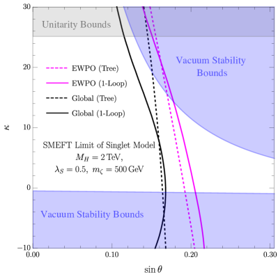
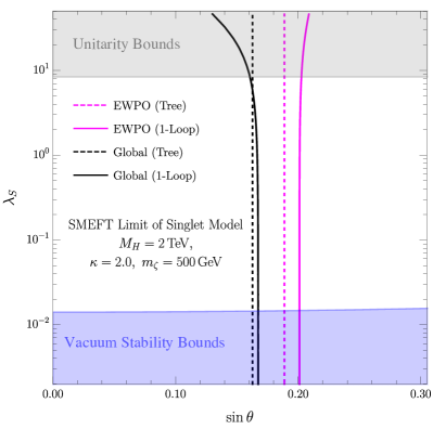
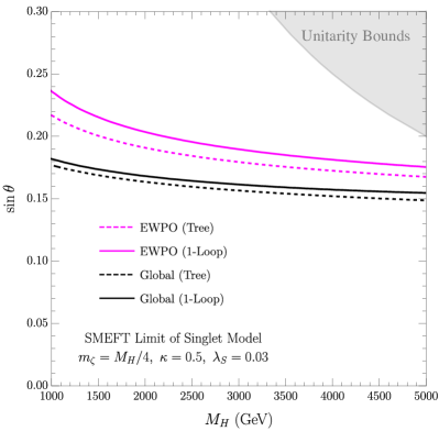
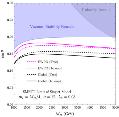
Figure 7: 95% C.L. limits on $\sin\theta$ as a function of $\kappa$ (LHS) and $\lambda_{S}$ (RHS) for fixed $M_{H}=2\,\textrm{TeV}$ and $m_{\zeta}=500\,\textrm{GeV}$. The fits with tree-level matching are shown as dashed curves, with solid curves showing the 1-loop result. The black curves show the result of a global fit to Higgs, diboson, and electroweak precision data, while the pink curves only the electroweak precision observables. The regions to the right of the curves are excluded by the fits. The grey and blue shaded regions are forbidden by unitarity and electroweak vacuum stability requirements, respectively.

Figure 8: As in Fig. 8, now showing limits on $\sin\theta$ as a function of the heavy Higgs mass, $M_{H}$, with fixed values of $\kappa$, $\lambda_{S}$ and $m_{\zeta}/M_{H}$. Regions above the curves are excluded.

Figs. 8 and 8 contain our major results. In terms of the parameters of the singlet model given in Eq. (3), we fix $M_{H}=2\,\textrm{TeV}$ and determine the maximum allowed value of $\sin\theta$ in terms of the other unknown parameters of the model, $\lambda_{S},~{}\kappa,$ and $m_{\zeta}$. The curves are relatively insensitive to $m_{\zeta}$ and $\lambda_{S}$ (RHS), and the major sensitivity is to $\kappa$ (LHS) of Fig. 8. We show the regions excluded by unitarity bounds and by vacuum stability bounds. The black curves include the Higgs, diboson, and EWPO data. For $\kappa\lesssim 8$, the inclusion of the 1-loop matching makes very little difference, but as $\kappa$ becomes large and approaches the unitarity bound, the difference between tree level and 1-loop matching can be of ${\cal{O}}(10\%)$. We separately show the limits from only EWPO limits in magenta and note that the 1-loop matching slightly improves the bound on $\sin\theta$.

Another interesting way to look at the results is to look at the maximum allowed value of $\sin\theta$ as a function of the heavy Higgs mass, $M_{H}$, for fixed values of $\kappa,m_{\zeta}$ and $\lambda_{S}$ as shown in Fig. 8. We see that including the 1-loop matching changes the bound on $\sin\theta$ only marginally. The effect is larger as $\kappa$ is increased.

Single parameter fits to models with an additional scalar have been presented in Ref. Ellis:2018gqa and updated in Ref. Ellis:2020unq using the dictionary of Ref. deBlas:2017xtg . Assuming $C_{H\square}=-1/M^{2}$ and $C_{H}=0$, they find a limit $M_{H}>900\,\textrm{GeV}$ at $2\sigma$. Our tree level matching result of Ref. Dawson:2020oco is roughly compatible with this bound, although we find that the inclusion of the renormalization group running of the coefficients (in particular $C_{HD}$ which is generated by renormalization group running) is numerically significant, so the bounds cannot be directly compared.

VI Conclusions

We have re-examined the sensitivity of a global fit to electroweak precision observables and to Higgs and diboson data on the parameters of a scalar singlet model in both the full UV complete model and in the low energy approximation where the heavy scalar is integrated out and the parameters are matched to the dimension-6 SMEFT. In the full singlet model, we find equivalent limits on the allowed mixing angle from the complete EWPO fit and from the fit to the oblique parameters when $M_{H}$ is heavy. For the case with the second Higgs boson much lighter than $M_{Z}$, the oblique parameter limits are not a good approximation to the full fit. When the new scalar is very heavy, we integrate it out and match to the dimension-6 SMEFT and then perform the global fit both using tree level and 1-loop matching at the high scale and derive limits on the parameters of the singlet theory from the SMEFT fit. We find that the effect on the fit of including the 1-loop matching is never larger than ${\cal{O}}(10\%)$ and that the results are quite insensitive to variations in the singlet Lagrangian parameters other than the portal term, $\kappa$.

Digital data can be found at https://quark.phy.bnl.gov/Digital_Data_Archive/dawson/singlet_21.

References

- (1) M. Bowen, Y. Cui, and J. D. Wells, “Narrow trans-TeV Higgs bosons and H hh decays: Two LHC search paths for a hidden sector Higgs boson,” JHEP 0703 (2007) 036, arXiv:hep-ph/0701035 [hep-ph].
- (2) D. O’Connell, M. J. Ramsey-Musolf, and M. B. Wise, “Minimal Extension of the Standard Model Scalar Sector,” Phys. Rev. D75 (2007) 037701, arXiv:hep-ph/0611014 [hep-ph].
- (3) S. Dawson and I. M. Lewis, “NLO corrections to double Higgs boson production in the Higgs singlet model,” Phys. Rev. D92 no. 9, (2015) 094023, arXiv:1508.05397 [hep-ph].
- (4) M. Mühlleitner, M. O. Sampaio, R. Santos, and J. Wittbrodt, “ScannerS: Parameter Scans in Extended Scalar Sectors,” arXiv:2007.02985 [hep-ph].
- (5) T. Robens and T. Stefaniak, “Status of the Higgs Singlet Extension of the Standard Model after LHC Run 1,” Eur.Phys.J. C75 no. 3, (2015) 104, arXiv:1501.02234 [hep-ph].
- (6) R. Costa, M. Mühlleitner, M. O. P. Sampaio, and R. Santos, “Singlet Extensions of the Standard Model at LHC Run 2: Benchmarks and Comparison with the NMSSM,” JHEP 06 (2016) 034, arXiv:1512.05355 [hep-ph].
- (7) C.-Y. Chen, S. Dawson, and I. M. Lewis, “Exploring resonant di-Higgs boson production in the Higgs singlet model,” Phys. Rev. D91 no. 3, (2015) 035015, arXiv:1410.5488 [hep-ph].
- (8) S. J. Huber, T. Konstandin, T. Prokopec, and M. G. Schmidt, “Electroweak Phase Transition and Baryogenesis in the nMSSM,” Nucl. Phys. B 757 (2006) 172–196, arXiv:hep-ph/0606298.
- (9) S. Profumo, M. J. Ramsey-Musolf, and G. Shaughnessy, “Singlet Higgs phenomenology and the electroweak phase transition,” JHEP 08 (2007) 010, arXiv:0705.2425 [hep-ph].
- (10) J. R. Espinosa, T. Konstandin, and F. Riva, “Strong Electroweak Phase Transitions in the Standard Model with a Singlet,” Nucl. Phys. B854 (2012) 592–630, arXiv:1107.5441 [hep-ph].
- (11) V. Barger, D. J. H. Chung, A. J. Long, and L.-T. Wang, “Strongly First Order Phase Transitions Near an Enhanced Discrete Symmetry Point,” Phys. Lett. B 710 (2012) 1–7, arXiv:1112.5460 [hep-ph].
- (12) S. Profumo, M. J. Ramsey-Musolf, C. L. Wainwright, and P. Winslow, “Singlet-catalyzed electroweak phase transitions and precision Higgs boson studies,” Phys. Rev. D91 no. 3, (2015) 035018, arXiv:1407.5342 [hep-ph].
- (13) D. Curtin, P. Meade, and C.-T. Yu, “Testing Electroweak Baryogenesis with Future Colliders,” JHEP 11 (2014) 127, arXiv:1409.0005 [hep-ph].
- (14) A. V. Kotwal, M. J. Ramsey-Musolf, J. M. No, and P. Winslow, “Singlet-catalyzed electroweak phase transitions in the 100 TeV frontier,” Phys. Rev. D94 no. 3, (2016) 035022, arXiv:1605.06123 [hep-ph].
- (15) T. Huang, J. M. No, L. Pernie, M. Ramsey-Musolf, A. Safonov, M. Spannowsky, and P. Winslow, “Resonant di-Higgs boson production in the channel: Probing the electroweak phase transition at the LHC,” Phys. Rev. D96 no. 3, (2017) 035007, arXiv:1701.04442 [hep-ph].
- (16) C.-Y. Chen, J. Kozaczuk, and I. M. Lewis, “Non-resonant Collider Signatures of a Singlet-Driven Electroweak Phase Transition,” JHEP 08 (2017) 096, arXiv:1704.05844 [hep-ph].
- (17) G. Kurup and M. Perelstein, “Dynamics of Electroweak Phase Transition In Singlet-Scalar Extension of the Standard Model,” Phys. Rev. D 96 no. 1, (2017) 015036, arXiv:1704.03381 [hep-ph].
- (18) H.-L. Li, M. Ramsey-Musolf, and S. Willocq, “Probing a scalar singlet-catalyzed electroweak phase transition with resonant di-Higgs boson production in the channel,” Phys. Rev. D100 no. 7, (2019) 075035, arXiv:1906.05289 [hep-ph].
- (19) N. Craig, C. Englert, and M. McCullough, “New Probe of Naturalness,” Phys. Rev. Lett. 111 no. 12, (2013) 121803, arXiv:1305.5251 [hep-ph].
- (20) D. Curtin and P. Saraswat, “Towards a No-Lose Theorem for Naturalness,” Phys. Rev. D 93 no. 5, (2016) 055044, arXiv:1509.04284 [hep-ph].
- (21) V. Silveira and A. Zee, “Scalar Phantoms,” Phys. Lett. B 161 (1985) 136–140.
- (22) J. McDonald, “Gauge singlet scalars as cold dark matter,” Phys. Rev. D 50 (1994) 3637–3649, arXiv:hep-ph/0702143.
- (23) C. P. Burgess, M. Pospelov, and T. ter Veldhuis, “The Minimal model of nonbaryonic dark matter: A Singlet scalar,” Nucl. Phys. B 619 (2001) 709–728, arXiv:hep-ph/0011335.
- (24) A. Menon, D. E. Morrissey, and C. E. M. Wagner, “Electroweak baryogenesis and dark matter in the nMSSM,” Phys. Rev. D 70 (2004) 035005, arXiv:hep-ph/0404184.
- (25) X.-G. He, T. Li, X.-Q. Li, J. Tandean, and H.-C. Tsai, “Constraints on Scalar Dark Matter from Direct Experimental Searches,” Phys. Rev. D 79 (2009) 023521, arXiv:0811.0658 [hep-ph].
- (26) M. Gonderinger, Y. Li, H. Patel, and M. J. Ramsey-Musolf, “Vacuum Stability, Perturbativity, and Scalar Singlet Dark Matter,” JHEP 01 (2010) 053, arXiv:0910.3167 [hep-ph].
- (27) Y. Mambrini, “Higgs searches and singlet scalar dark matter: Combined constraints from XENON 100 and the LHC,” Phys. Rev. D 84 (2011) 115017, arXiv:1108.0671 [hep-ph].
- (28) S. Dawson, S. Homiller, and S. D. Lane, “Putting standard model EFT fits to work,” Phys. Rev. D 102 no. 5, (2020) 055012, arXiv:2007.01296 [hep-ph].
- (29) J. Brehmer, A. Freitas, D. Lopez-Val, and T. Plehn, “Pushing Higgs Effective Theory to its Limits,” Phys. Rev. D93 no. 7, (2016) 075014, arXiv:1510.03443 [hep-ph].
- (30) B. Henning, X. Lu, and H. Murayama, “What do precision Higgs measurements buy us?,” arXiv:1404.1058 [hep-ph].
- (31) B. Henning, X. Lu, and H. Murayama, “How to use the Standard Model effective field theory,” JHEP 01 (2016) 023, arXiv:1412.1837 [hep-ph].
- (32) M. Gorbahn, J. M. No, and V. Sanz, “Benchmarks for Higgs Effective Theory: Extended Higgs Sectors,” JHEP 10 (2015) 036, arXiv:1502.07352 [hep-ph].
- (33) J. Ellis, C. W. Murphy, V. Sanz, and T. You, “Updated Global SMEFT Fit to Higgs, Diboson and Electroweak Data,” JHEP 06 (2018) 146, arXiv:1803.03252 [hep-ph].
- (34) J. Ellis, M. Madigan, K. Mimasu, V. Sanz, and T. You, “Top, Higgs, Diboson and Electroweak Fit to the Standard Model Effective Field Theory,” arXiv:2012.02779 [hep-ph].
- (35) Anisha, S. Das Bakshi, J. Chakrabortty, and S. K. Patra, “A Step Toward Model Comparison: Connecting Electroweak-Scale Observables to BSM through EFT and Bayesian Statistics,” arXiv:2010.04088 [hep-ph].
- (36) D. Egana-Ugrinovic and S. Thomas, “Effective Theory of Higgs Sector Vacuum States,” arXiv:1512.00144 [hep-ph].
- (37) S. Das Bakshi, J. Chakrabortty, and M. Spannowsky, “Classifying Standard Model Extensions Effectively with Precision Observables,” arXiv:2012.03839 [hep-ph].
- (38) G. D. Kribs, A. Maier, H. Rzehak, M. Spannowsky, and P. Waite, “Electroweak oblique parameters as a probe of the trilinear Higgs boson self-interaction,” Phys. Rev. D 95 no. 9, (2017) 093004, arXiv:1702.07678 [hep-ph].
- (39) A. Falkowski, C. Gross, and O. Lebedev, “A second Higgs from the Higgs portal,” JHEP 05 (2015) 057, arXiv:1502.01361 [hep-ph].
- (40) M. Jiang, N. Craig, Y.-Y. Li, and D. Sutherland, “Complete One-Loop Matching for a Singlet Scalar in the Standard Model EFT,” JHEP 02 (2019) 031, arXiv:1811.08878 [hep-ph]. [Erratum: JHEP 01, 135 (2021)].
- (41) U. Haisch, M. Ruhdorfer, E. Salvioni, E. Venturini, and A. Weiler, “Singlet night in Feynman-ville: one-loop matching of a real scalar,” JHEP 04 (2020) 164, arXiv:2003.05936 [hep-ph]. [Erratum: JHEP 07, 066 (2020)].
- (42) T. Cohen, X. Lu, and Z. Zhang, “Functional Prescription for EFT Matching,” arXiv:2011.02484 [hep-ph].
- (43) G. Buchalla, O. Cata, A. Celis, and C. Krause, “Standard Model Extended by a Heavy Singlet: Linear vs. Nonlinear EFT,” Nucl. Phys. B917 (2017) 209–233, arXiv:1608.03564 [hep-ph].
- (44) S. Dawson, A. Ismail, and I. Low, “What’s in the loop? The anatomy of double Higgs production,” Phys. Rev. D 91 no. 11, (2015) 115008, arXiv:1504.05596 [hep-ph].
- (45) ATLAS Collaboration, G. Aad et al., “Combined measurements of Higgs boson production and decay using up to fb-1 of proton-proton collision data at 13 TeV collected with the ATLAS experiment,” Phys. Rev. D 101 no. 1, (2020) 012002, arXiv:1909.02845 [hep-ex].
- (46) CMS Collaboration, “Combined Higgs boson production and decay measurements with up to fb-1 of proton-proton collision data at = 13 TeV,”. https://cds.cern.ch/record/2706103.
- (47) ATLAS Collaboration, G. Aad et al., “Combination of searches for Higgs boson pairs in collisions at 13 TeV with the ATLAS detector,” Phys. Lett. B 800 (2020) 135103, arXiv:1906.02025 [hep-ex].
- (48) W. F. L. Hollik, “Radiative Corrections in the Standard Model and their Role for Precision Tests of the Electroweak Theory,” Fortsch. Phys. 38 (1990) 165–260.
- (49) A. Freitas, “Higher-order electroweak corrections to the partial widths and branching ratios of the Z boson,” JHEP 04 (2014) 070, arXiv:1401.2447 [hep-ph].
- (50) S. Dawson and P. P. Giardino, “Electroweak and QCD corrections to and pole observables in the standard model EFT,” Phys. Rev. D 101 no. 1, (2020) 013001, arXiv:1909.02000 [hep-ph].
- (51) S. Carrazza, R. K. Ellis, and G. Zanderighi, “QCDLoop: a comprehensive framework for one-loop scalar integrals,” Comput. Phys. Commun. 209 (2016) 134–143, arXiv:1605.03181 [hep-ph].
- (52) D. Lopez-Val and T. Robens, “ r and the W-boson mass in the singlet extension of the standard model,” Phys. Rev. D90 no. 11, (2014) 114018, arXiv:1406.1043 [hep-ph].
- (53) S. Dawson and W. Yan, “Hiding the Higgs Boson with Multiple Scalars,” Phys. Rev. D79 (2009) 095002, arXiv:0904.2005 [hep-ph].
- (54) C. Englert, J. Jaeckel, M. Spannowsky, and P. Stylianou, “Power meets Precision to explore the Symmetric Higgs Portal,” Phys. Lett. B 806 (2020) 135526, arXiv:2002.07823 [hep-ph].
- (55) M. E. Peskin and T. Takeuchi, “Estimation of oblique electroweak corrections,” Phys. Rev. D 46 (1992) 381–409.
- (56) Particle Data Group Collaboration, P. Zyla et al., “Review of Particle Physics,” PTEP 2020 no. 8, (2020) 083C01.
- (57) A. Ilnicka, T. Robens, and T. Stefaniak, “Constraining Extended Scalar Sectors at the LHC and beyond,” Mod. Phys. Lett. A33 no. 10n11, (2018) 1830007, arXiv:1803.03594 [hep-ph].
- (58) G. Chalons, D. Lopez-Val, T. Robens, and T. Stefaniak, “The Higgs singlet extension at LHC Run 2,” PoS DIS2016 (2016) 113, arXiv:1606.07793 [hep-ph].
- (59) J. de Blas, M. Ciuchini, E. Franco, S. Mishima, M. Pierini, L. Reina, and L. Silvestrini, “The Global Electroweak and Higgs Fits in the LHC era,” PoS EPS-HEP2017 (2017) 467, arXiv:1710.05402 [hep-ph].
- (60) T. Robens and T. Stefaniak, “LHC Benchmark Scenarios for the Real Higgs Singlet Extension of the Standard Model,” Eur. Phys. J. C 76 no. 5, (2016) 268, arXiv:1601.07880 [hep-ph].
- (61) B. W. Lee, C. Quigg, and H. Thacker, “The Strength of Weak Interactions at Very High-Energies and the Higgs Boson Mass,” Phys. Rev. Lett. 38 (1977) 883–885.
- (62) B. W. Lee, C. Quigg, and H. Thacker, “Weak Interactions at Very High-Energies: The Role of the Higgs Boson Mass,” Phys. Rev. D 16 (1977) 1519.
- (63) S. Dawson and C. W. Murphy, “Standard Model EFT and Extended Scalar Sectors,” Phys. Rev. D96 no. 1, (2017) 015041, arXiv:1704.07851 [hep-ph].
- (64) W. Buchmuller and D. Wyler, “Effective Lagrangian Analysis of New Interactions and Flavor Conservation,” Nucl. Phys. B 268 (1986) 621–653.
- (65) A. Dedes, W. Materkowska, M. Paraskevas, J. Rosiek, and K. Suxho, “Feynman rules for the Standard Model Effective Field Theory in -gauges,” JHEP 06 (2017) 143, arXiv:1704.03888 [hep-ph].
- (66) J. de Blas, J. C. Criado, M. Perez-Victoria, and J. Santiago, “Effective description of general extensions of the Standard Model: the complete tree-level dictionary,” JHEP 03 (2018) 109, arXiv:1711.10391 [hep-ph].
- (67) E. E. Jenkins, A. V. Manohar, and M. Trott, “Renormalization Group Evolution of the Standard Model Dimension Six Operators I: Formalism and lambda Dependence,” JHEP 10 (2013) 087, arXiv:1308.2627 [hep-ph].
- (68) E. E. Jenkins, A. V. Manohar, and M. Trott, “Renormalization Group Evolution of the Standard Model Dimension Six Operators II: Yukawa Dependence,” JHEP 01 (2014) 035, arXiv:1310.4838 [hep-ph].
- (69) R. Alonso, E. E. Jenkins, A. V. Manohar, and M. Trott, “Renormalization Group Evolution of the Standard Model Dimension Six Operators III: Gauge Coupling Dependence and Phenomenology,” JHEP 04 (2014) 159, arXiv:1312.2014 [hep-ph].
- (70) G. Degrassi, M. Fedele, and P. P. Giardino, “Constraints on the trilinear Higgs self coupling from precision observables,” JHEP 04 (2017) 155, arXiv:1702.01737 [hep-ph].
- (71) G. Degrassi, P. P. Giardino, F. Maltoni, and D. Pagani, “Probing the Higgs self coupling via single Higgs production at the LHC,” JHEP 12 (2016) 080, arXiv:1607.04251 [hep-ph].
- (72) J. Baglio, S. Dawson, and S. Homiller, “QCD corrections in Standard Model EFT fits to and production,” Phys. Rev. D 100 no. 11, (2019) 113010, arXiv:1909.11576 [hep-ph].
- (73) J. Baglio, S. Dawson, S. Homiller, S. D. Lane, and I. M. Lewis, “Validity of standard model EFT studies of VH and VV production at NLO,” Phys. Rev. D 101 no. 11, (2020) 115004, arXiv:2003.07862 [hep-ph].