Noisy multistate voter model for flocking in finite dimensions
Abstract
We study a model for the collective behavior of self-propelled particles subject to pairwise copying interactions and noise. Particles move at a constant speed on a two–dimensional space and, in a single step of the dynamics, each particle adopts the direction of motion of a randomly chosen neighboring particle within a distance , with the addition of a perturbation of amplitude (noise). We investigate how the global level of particles’ alignment (order) is affected by their motion and the noise amplitude . In the static case scenario where particles are fixed at the sites of a square lattice and interact with their first neighbors, we find that for any noise the system reaches a steady state of complete disorder in the thermodynamic limit, while for full order is eventually achieved for a system with any number of particles . Therefore, the model displays a transition at zero noise when particles are static, and thus there are no ordered steady states for a finite noise (). We show that the finite-size transition noise vanishes with as and in one and two–dimensional lattices, respectively, which is linked to known results on the behavior of a type of noisy voter model for catalytic reactions. When particles are allowed to move in the space at a finite speed , an ordered phase emerges, characterized by a fraction of particles moving in a similar direction. The system exhibits an order-disorder phase transition at a noise amplitude that is proportional to , and that scales approximately as for . These results show that the motion of particles is able to sustain a state of global order in a system with voter-like interactions.
I Introduction
The study of the collective properties of systems composed by self-propelled individuals has been the focus of intense research in the last two decades vicsek2012 ; marchetti2013 ; menzel2015 . The flocking behavior of a large group of animals is observed in many different species such as fish, birds, bacteria and insects, among others. From a statistical physics viewpoint, the interactions between particles in a system are responsible of its collective behavior, and lead to well characterized classes represented by archetype models. For the case of flocking, the alignment interaction among individuals is usually modeled as a local averaging of moving directions of nearby individuals, plus a noise that accounts for errors in the average process vicsek-1995 . A crucial role in the emergent behavior of the system is played by the displacement of the individuals, which changes dramatically its ordering properties toner-1995 .
Within the context of flocking, the dynamics of collective alignment in groups of fish was recently studied in jhawar2020 . The authors performed experiments with cichlid fish Etroplus suratensis that swim in a circular shallow tank, in order to explore how schooling is affected by the fish group size. The level of group alignment is quantified by a vector order parameter that is the average velocity of fish, also called group polarization, in such a way that corresponds to a polarized state where fish move in a coherent direction, while represents a collectively disordered state –each fish moving in a random direction. Performing the experiments for group sizes , and , they found that the collective alignment increases as decreases. An insight into this phenomenon is given by a phenomenological stochastic differential equation (SDE) for the time evolution of , where its parameters were extracted from the experimental data. It is shown that group polarization is the result of the interplay between the drift and the demographic (population) noise terms in the SDE, that is, the fewer the fish, the greater the demographic noise and so the greater the alignment level. Thus, they conclude that schooling (highly polarized and coherent motion) is induced by the intrinsic population noise that arises from the stochasticity related to the finite number of interacting fish. They derived the SDE for by means of a mean-field (MF) model in which particles (fish) interact by pairs and follow a simple imitation dynamics: each particle either copies the direction of another random particle or spontaneously changes its direction, modeled as an external noise of amplitude . They also show that other ternary or higher-order aligning interactions, including local averages like in the Vicsek-like family of models, are unnecessary to explain these experimental results. Therefore, they arrive to the conclusion that the minimal theoretical mechanism that reproduces the collective alignment properties of fish observed in the experiments is that of pairwise interactions with copying dynamics and noise. We notice that the noiseless version of this particular alignment dynamics that induces flocking was first introduced in baglietto2018 , where the authors study the collective motion of particles on a two–dimensional () space subject to voter-like interactions, that is, each particle aligns its direction of motion with that of a random neighboring particle within an interaction radius.
From the theoretical point of view, an interesting result can be inferred from the work in jhawar2020 by analyzing the SDE for the group polarization . That is, this equation predicts complete order () for zero noise () and full disorder () for any finite noise amplitude in the limit. This observation is in agreement with recent analytical results obtained in a similar model with a discrete set of angular directions, a multistate voter model (MSVM) with external noise Vazquez-2019 , where it is shown that the order parameter approaches as in the limit, and vanishes when increases as for any . Thus, the partial order obtained with voter interactions and noise in a MF set up is only a finite size effect that eventually disappears in the thermodynamic limit. These results suggest a peculiar order-disorder transition at zero noise, unseen in related flocking models such as the binary Vicsek model Chou-2015 where each particle averages its direction with that of other random particle, and the transition happens at a critical noise larger than zero. However, we notice that the experimental results obtained in jhawar2020 correspond to fish moving on a set up (tank), while both the SDE and the model in Vazquez-2019 are for a MF set up (infinite dimension), where every particle interacts with any other particle, and thus motion plays no role in the dynamics. It is natural, therefore, to wonder whether these results hold when particles move on a space. Do space and motion affect the transition at zero noise?
In this article we study a noisy multistate voter model for flocking in finite dimensions, and we investigate the order-disorder phase transition in different case scenarios. We start by analyzing the simplest case of all-to-all interactions or MF. We then explore the static case where each particle occupies a site of a square lattice and interacts with its first nearest-neighbors, and we finally study the dynamic case in which particles move on a continuous space and change their direction when they interact with other nearby particles that are located within a distance . In the case that particles are allowed to have only two possible angular states and interact on a MF set up, the model turns to be equivalent to the noisy voter model (NVM) introduced in Kirman-1993 ; Granovsky-1995 , in which each individual of a population holds one of two states (opinions) that are updated by either copying the state of a random neighbor or spontaneously switching state (noise). In the absence of noise, any finite population eventually reaches full order (consensus) in all dimensions, as in the original voter model clifford1973 ; holley1975 , with all individuals sharing the same opinion. However, the addition of a weak noise leads to a bi-stable regime in which the system jumps between two steady states corresponding to a quasi-consensus in one or the other opinion Kirman-1993 ; Granovsky-1995 , while for strong noise the system remains disordered. This is in line with the fact that adding thermal bulk noise in the voter model destroys global order in any dimension Henkel-2008 , even when the noise is weak. In square lattices, the NVM is equivalent to a particular limit of the catalytic reaction model with desorption originally introduced in Fichthorn-1988 and widely studied after Fichthorn-1989 ; Considine-1989 , which exhibits a finite size transition induced by noise called saturation transition Clement-1991a ; Clement-1991b ; Flament-1992 . More recently, the dynamics of the NVM has been investigated in complex networks Carro-2016 ; Peralta-2018-a ; Peralta-2018-b , and its version with multiple states has been explored in fully connected systems Azque-2019 ; Vazquez-2019 . Also, an asymmetric variant of the NVM with long-range interactions has recently been proposed to study the competition between two species for territory Martinez-2020 .
While in lattice models bulk noise inhibits the formation of long range order in the thermodynamic limit, it is known that in flocking systems the displacement of particles plays an ordering role. This ordering phenomenon is observed in the Vicsek model, thought as a non equilibrium version of the XY model in with particles moving ballistically in the directions of their spins. That is, while the Vicsek model can sustain long-range order for finite values of noise amplitude due to particles’ motion toner-1995 , the XY model is unable to do so MWtheorem-1966 . Then, the velocity of particles in Vicsek-type models leads to steady states associated with a new ordered phase below a transition noise . However, voter-type interactions (copying) are different from Vicsek-type interactions (averaging), leading to different behaviors in MF and three dimensions: long-range order in the XY model, and disorder in the NVM. Therefore, in the flocking voter model (FVM) studied in this article, we expect a non-trivial competition between the ordering mechanism generated by particles’ motion and the typical disordering effect induced by noisy voter interactions that leads to complete disorder in the thermodynamic limit. Thus, we aim to explore whether the ordered phase observed in flocking models is still present in the FVM, or it is rather completely suppressed by noise.
The rest of the article is organized as follows. In section II we define the model. Section III presents MF results, while section IV is dedicated to the static version of the model in one and two dimensional square lattices. In section V we study the dynamic version of the model in a continuous space. We investigate the effects of particles’ velocity in the transition, with a particular focus on the behavior at low speeds in the thermodynamic limit. Finally, in section VI we summarize and give some conclusions.
II The model
A set of particles are allowed to move at a constant speed on a square box of side with periodic boundary conditions. The position and velocity of particle () at time are denoted by and , respectively, where is the particle’s speed and is its angular moving direction. The density of particles is fixed at in our analysis, unless stated. Initially, each particle adopts a random position inside the box and points in a random direction. In a given time step of the dynamics, each particle updates it position and direction according to
| (1a) | ||||
| (1b) | ||||
where is the moving direction of a randomly chosen particle that is inside a disk of radius centered at , and is a random angle drawn uniformly in with amplitude (). This update is performed for all particles at the same time (parallel update). That is, each particle moves at a constant speed following a given straight path and updates its direction at integer times , by adopting the direction of a random neighboring particle with an error of amplitude . If a particle has no neighbors inside its interaction range , then its direction is changed only by the noise .
In flocking models, noise –in its various forms– plays a fundamental role in the behavior of the system. It is known that the amplitude of noise induces an order-disorder phase transition, from a phase where a large fraction of particles move in a similar direction (order) for small , to a phase in which particles move in random directions (disorder) for large . To study this phenomenon in the FVM we define the order parameter (see for instance jhawar2020 ; baglietto2018 )
| (2) |
that measures the level of collective alignment in the system (magnitude of the normalized mean velocity of all particles), and the susceptibility
| (3) |
which accounts for the amplitude of fluctuations of at the stationary state. Here is the -th moment of , and the symbol represents the average value of a given magnitude over many realizations of the dynamics at the steady state.
Our aim is to explore via computational simulations and scaling theory how space and motion affects the phase transition in the FVM. For that, we first study the model in MF (), we then explore the static case in lattices, and we finally investigate the dynamic case in .
III Mean Field
In order to gain an insight into the behavior of the FVM, we start by analyzing in this section the simplest case scenario of all-to-all interactions or MF, which corresponds to the large interaction range limit of the model defined in section II. In this case, the dynamics of the angular directions of particles is independent of the positions of particles, and thus it is entirely determined by Eq. (1b). That is, each particle simply adopts the direction of another randomly chosen particle in the system, with the addition of noise. This dynamics is equivalent to that of the multistate voter model with imperfect copying introduced and studied in Vazquez-2019 , in the limit of continuum angular states. In a single time step , a particle with state is picked at random, then it copies the state of another randomly chosen particle , and this state is slightly perturbed:
| (4) |
We note that we are implementing here a sequential update in which only one particle updates its state in a time step, unlike the parallel update where all particles are updated at once. However, we have verified that the behavior of the macroscopic variables and under the parallel update is recovered by making the substitution in the results obtained with the sequential update, as mathematically proved by Blythe and McKane in Blythe-2007 for population genetic models akin to the voter model. Inversely, the transformation allows to obtain the behavior under the sequential update from the results with parallel update.
|
|
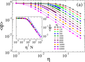
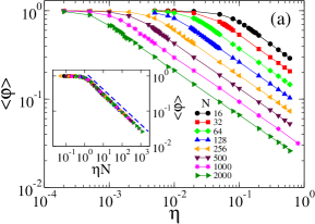
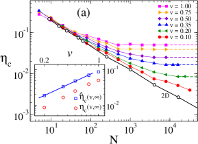
Figure 1 shows simulation results for the model in MF. Data points correspond to average values in a time interval after the system reached the stationary state, between times and , and over independent realizations. In panel (a) we observe that the order parameter continuously decreases as increases, and that approaches the value (full order) as , which corresponds to the absorbing consensus state obtained in the zero noise case , as it is known from previous works of the multistate voter model Starnini-2012 ; Pickering-2016 ; baglietto2018 ; Vazquez-2019 . We also see that, for a fixed value of , vanishes as the system size increases, suggesting that for any in the limit. Indeed, an expression for the scaling of with and that confirms this assumption can be obtained from analytical results of this model recently presented in Vazquez-2019 , for an order parameter . It was shown in Vazquez-2019 that for and , and thus assuming we obtain the approximate MF behavior
| (5) |
In the inset of Fig. 1(a) we plot the data as a function of the scaling variable , where we can see that obeys the power law decay from Eq. (5) for (dashed line). We also observe a good collapse of the curves for different system sizes in the entire range of , showing that the order parameter is a function of , , with for .
|
|
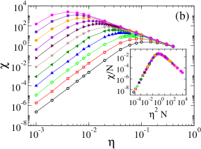
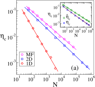
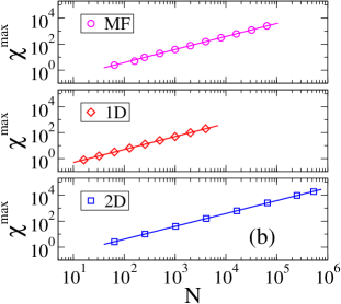
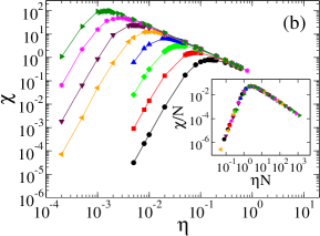
The results above imply that in the absence of noise the system reaches full order (), but a tiny amount of noise is enough to drive the system to complete disorder () in the thermodynamic limit, which suggests a transition at zero noise. To study this in more detail, we show in Fig. 1(b) the behavior of the susceptibility with . We observe that the curve for a given system size exhibits a maximum that is an indication of a transition that depends on , between an ordered phase for and a disordered phase for , where the transition point is estimated as the location of the peak. In Fig. 2(a) we plot the transition noise vs (circles), where we can see that vanishes as increases following a power-law behavior , with a best fitting exponent . This implies a transition value in the thermodynamic limit. In panel (b) of Fig. 2 we see that the maximum value of the susceptibility increases with as , where is the best fitting exponent.
These scalings can be nicely verified by assuming that is also a function of the scaling variable for in Fig. 1. Indeed, rescaling the –axis of Fig. 1(b) by and plotting the resulting data vs we find a good collapse of all curves for different values (see inset), showing that the MF susceptibility behaves as
| (6) |
where is a smooth function of . From Eq. (6) we have that at the MF transition point is and, therefore,
| (7) |
in agreement with numerical results [Fig. 2(a)].
In summary, the mean field version of the FVM exhibits an order-disorder phase transition at zero noise in the thermodynamic limit, between a perfectly ordered phase where for and a completely disordered phase where for .
IV Static case in one and two dimensions
In this section we analyze the static version of the FVM in finite dimensions. For that, we consider that each particle occupies a site of a square lattice of length and dimensions ( sites), and interacts with its nearest neighbors only. We have simulated the dynamics of the model under the sequential update described in section III on lattices of dimensions and with periodic boundary conditions. In a time step , a randomly selected particle copies the angular state of a first neighbor chosen at random, with the addition of an error of amplitude .
|
|
Figure 3 shows simulation results for the FVM in one dimension. The behavior of and are similar to those of the MF model, with a scaling variable in this one–dimensional case. The variable was obtained from the behavior of the transition noise with given by the peak of in panel (b) of Fig. 3. We found , with [Fig. 2(a)], while for the peak of the susceptibility we found the scaling , with [Fig. 2(b)]. Therefore, assuming the scalings
| (8) | |||||
| (9) |
we arrive at the following scaling for the susceptibility:
| (10) |
and thus the scaling variable is , as stated above. Indeed, we can check in the insets of Fig. 3 the collapse of the curves for different system sizes when the data is plotted vs , and the –axis in panel (b) is rescaled by . Also, in the inset of panel (a) we show that the order parameter scales as for (dashed line), which exhibits the same behavior with respect to the scaling variable as that of MF [Eq. (5)], i.e., a power-law decay with exponent .
The scaling relation Eq. (8) shows that the transition noise vanishes with and, therefore, we conclude that the static version of the FVM in one dimension exhibits an order-disorder transition at zero noise in the thermodynamic limit, as it happens in MF.

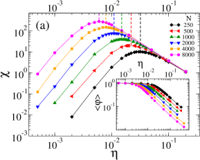
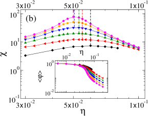
We repeated the same analysis for the FVM model on two dimensional lattices. Simulation results are presented in Fig. 4, where the data collapse was obtained by means of two different scaling variables, as we describe below. As it happens for the MF and the cases, the transition noise (given by the maximum of the susceptibility) decays as a power law with the system size as [square symbols in Fig. 2(a)], with a best power-law fitting exponent . Even though this exponent is different from the MF and exponents and , respectively, this numerical scaling implies an extrapolated transition noise in the limit. The peak of the susceptibility seems to increase linearly with as in MF and , with a best-fitting exponent [Fig. 2(b)]. Based on these results, we plot and as a function of in Figs. 4(a) and (b), respectively, where we observe a good collapse of curves for different system sizes. For the sake of simple comparison, we have also collapsed the same data using the MF scaling variable instead, and found that the data points do not fall into a single curve but they look rather disperse (plot not shown). Therefore, we conclude that the case appears to have its own scaling variable, which is proportional to a non-trivial power of .
A more appealing scaling variable can be obtained from known results of the behavior of the surface-reaction model introduced by Fichthorn, Gulari and Ziff (FGZ) in Fichthorn-1989 and studied later in Clement-1991a ; Clement-1991a ; Clement-1991b ; Flament-1992 , akin to the two-state NVM Kirman-1993 ; Granovsky-1995 , which be believe it belongs to the same class of the MSVM for flocking studied here. In the FGZ model, particles of two different species and occupy the sites of a square lattice that simulates a catalytic substrate. In a single step, two possible reaction events can take place. (i) With probability one particle is chosen at random and desorbs, and the vacant site is immediately occupied with a particle of species or with the same probability . This corresponds to the external noise of the NVM that switches the state of a particle with probability . (ii) With the complementary probability a pair of neighboring sites is chosen at random and, if it is an pair, both particles desorb and are replaced with an or a pair, equiprobably. This represents the copy dynamics of the NVM. The control parameter of the FGZ model is the desorption probability (noise amplitude). The steady state at is a poisoned absorbing state with a coverage equals to (all particles in state or ), which is analogous to complete order for in the FVM. For the coverage is smaller than , depending on the values of and , similarly to the partial order in the FVM.
It turns out that the scaling variables that we obtained for the FVM in MF and are the same as those of the FGZ model, by making a suitable change of variables. In the FGZ model they obtained analytically the scaling variables in MF () and in Clement-1991a ; Clement-1991b , while in the FVM are in MF and in . Thus, the scaling variables of both models match if we make the substitution . Finally, is a marginal dimension in the FGZ model, with a scaling variable similar to that of MF with a logarithmic correction in , that is, . Therefore, for the FVM in we expect a scaling variable , where we have defined an effective noise amplitude .
Panels (c) and (d) of Fig.4 show and plotted as a function of the scaling variable , where we see a good data collapse. Even though this collapse with seems as good as that with [panels (a) and (b)], the advantage of using is two fold: we are not fitting any parameter and we recover the linear dependence on found in MF and scaling variables and . Additionally, Fig. 4(c) shows that the order parameter scales as for (dashed line), consistent with the power law decay found in MF and . In comparison, decays as a power law of with a non-trivial exponent [dashed line in Fig. 4(a)]. Finally, from the scaling relation for the susceptibility
| (11) |
where is a smooth function of [see Fig. 4(d)], we obtain the effective transition noise
| (12) |
in , where is a proportionality constant. Interestingly, the exponent in the case agrees with that of the MF case [Eq. (7)]. In the inset of Fig. 2(a) we compare the effective transition noise
| (13) |
from simulations (circles) with the approximate scaling given by Eq. (12) (upper solid line), with a best fitting constant . The good agreement between simulations and Eq. (12) shows that the transformation of the original noise into the effective noise leads to power-law decay in with a MF exponent .
We can now obtain an approximate expression for the transition noise assuming that it has the power law behavior as found numerically [squares in Fig. 2(a)], where the exponent depends on and is a constant obtained from the fitting of the data. Starting from the relation Eq. (13) between the effective and original noise, we apply the logarithm at both sides and replace by from Eq. (12) and by , which leads to
| (14) |
after doing some algebra and rearranging terms. We have also considered the expansion to zero-th order in , as we can check for , , and . Then, as we expect to be similar to ( from the fitting of the data in Fig. 2), we replace in Eq. (14) by the Taylor expansion , and solve for . We finally arrive at the following approximate scaling for the transition noise with :
| (15a) | ||||
| (15b) | ||||
| (15c) | ||||
using . In the inset of Fig. 2 we can see that the approximation from Eq. (15c) (bottom solid curve) reproduces very well the behavior of vs from simulations (squares). The second term in the exponent [Eq. (15b)] leads to a very slow curvature in log-log scale with an effective exponent in the shown range of , which approaches very slowly to the value as increases. Finally, from Eq. (15c) we can see that the transition point vanishes in the limit.
Summarizing the results of this section, the static version of the FVM in one and two– dimensional lattices exhibits an order-disorder transition at zero noise in the thermodynamic limit.
V Dynamic case in two dimensions
When particles are allowed to move over the space, their speed becomes a relevant parameter that drastically changes the behavior of the system respect to the static case analyzed in section IV, as we shall see below. Simulations were done on a two–dimensional continuous space (square box) using the parallel dynamics defined in section II. We remark that interactions are local, that is, each particle can only interact with other particles that are less than a distance apart, by copying the direction of one of them chosen at random.
|
|
In Fig. 5 we plot the susceptibility and the order parameter (inset) vs noise amplitude for speeds [panel (a)] and [panel (b)]. In principle, we observe a behavior similar to that of MF and the and static cases studied previously where decays monotonically with , and exhibits a maximum at a value that decreases with , as we can clearly see for . However, an inspection of the plot reveals that appears to decrease and saturate at a minimum value as increases, unlike in MF and the static cases where vanishes with . Also, if we compare the level of order and its fluctuations for the two speeds, we can see a larger order with smaller fluctuations for the largest speed , suggesting that the speed has an ordering effect.
To look at this in more detail, we plot in Fig. 6 the transition noise vs the system size for different speeds. Indeed, for a given speed , we can see that exhibits a decay similar to a power law for small values of , and saturates at a minimum value for large , which decreases as decreases. We also plot for comparison the transition noise for the static case in two–dimensional lattices (empty circles). For the sake of clarity, the dashed line has been shifted in the -axis to match the estimated asymptotic behavior of in the zero speed limit , as we do not expect and to be exactly the same. This is because some macroscopic magnitudes of the dynamic model (, and ) depend on other variables besides and , such as the density of particles .
|
|
The numerical results described above show that, in the thermodynamic limit, there is an order-disorder transition at a finite noise amplitude that increases with the speed . To study this transition in more detail, we investigate below the scaling behavior of with the speed and the system size.
Since we have learned in section IV that working with an effective noise in lattices leads to scalings with simple MF exponents, it seems reasonable to explore the data of Fig. 6 for an effective transition noise
| (16) |
which incorporates a correction factor to the original noise . The approximate power-law decay of for small and its saturation for large [Fig. 6(a)] suggests that the scaling behavior of could be described by the following standard Family-Vicsek function with two independent exponents and Family-Vicsek-1985 :
| (17) |
where is a scaling function with the asymptotic properties
| (18) |
We can check that Eq. (17) exhibits the two limiting behaviors
| (19) |
in the thermodynamic limit, and
| (20) |
in the zero speed limit, where the exponent satisfies the relation
| (21) |
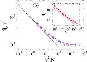
By means of the scaling relation Eq. (17) we can collapse the data points of Fig. 6 into a single curve. For that, we first estimate the exponents , and . From the plot vs in the inset of Fig. 6 (squares) we find the best power-law fitting (straight line), where and . Then, in the zero speed limit we assume that takes the value of the static case, and thus we obtain from Eq. (21). Based on these exponents, we propose the following scaling for the effective transition noise:
| (22) |
with for and for . Figure 6(b) shows a good data collapse obtained with the scaling Eq. (22). Remarkably, this result only required the estimation of the best fitting exponent of the vs data, and assuming that the scaling of the transition noise with N in the zero speed limit is the same as that of the static case.
The effective transition noise given by Eq. (22) scales linearly with the speed in the thermodynamic limit,
| (23) |
where is the best fitting constant for low speeds [straight line in the inset of Fig. 6(a)]. An approximate power-law scaling for the original noise can be obtained by following the same approach described in section IV to obtain the scaling of with [Eq. (15)]. For that, we start from the relation between and in logarithmic scale and replace by [Eq. (23)] and by . After rearranging terms and making the approximation to zero-th order in we arrive at
| (24) |
As we expect to be similar to [circles in the inset of Fig. 6(a)], we use the linear approximation in Eq. (24) and solve for . We finally obtain the following approximate expressions for the transition noise:
| (25a) | ||||
| (25b) | ||||
| (25c) | ||||
The second term in Eq. (25b) gives an effective exponent that decreases and approaches the value very slowly as decreases. Equations (25) are only valid for low speeds due to the fact that the approximate expansion of the logarithm that we used in Eq. (24) assumes that , which happens for . Unfortunately, the comparison of Eq. (25) with simulation results is not possible because to obtain the numerical value for speeds is extremely costly in terms of simulation running times.
Equation (22) also implies the scaling
| (26) |
which is confirmed in Fig. 6(b), where the collapsed data exhibits an approximate power law decay with exponent for , denoted by the dashed line. Finally, in the inset of Fig. 6(b) we compare the curve vs for the lowest speed with the scaling (dashed line). A good agreement is observed only at intermediate values of , while for small or large sizes a deviation from the slope becomes clear. We understand that the discrepancy for small is due to the absence of the logarithmic correction that becomes more relevant as decreases, while for large we expect that reaches a saturation at a minimum value . This asymptotic value of is reached for system sizes outside the shown range and, in general, the approximate system size from where we start to see a plateau in seems to diverge as approaches zero [see Fig. 6(a)]. An insight into this can be given in terms of the crossover size that separates the two limiting behaviors of for small and large . For the effective transition noise decays with as , while for is . At the crossover size, these two limiting scalings should match, leading to . This simple relation shows that, as approaches zero, the crossover size diverges very fast, and so we need to run simulations in very large systems to observe the asymptotic value of .
In summary, we showed in this section that the FVM in a continuous space exhibits and order-disorder phase transition at a finite noise amplitude that is proportional to the speed of particles. For low speeds, is linear in with a logarithmic correction that leads to an effective power law with a –dependent exponent slightly larger than . Thus, the transition at a finite noise induced by particles’ motion is in contrast with the zero-noise transition found in MF and the static version of the model in lattices.
VI Summary and Conclusions
We studied a model for the flocking dynamics of self-propelled particles with pairwise copying interactions and noise. This model can be considered as a version of the noisy voter model with infinite number of angular states, which also incorporates the motion of particles over the space. We focused on the ordering properties of the system by exploring the order parameter that measures the global level of alignment of particles. We found that the system undergoes a transition as the noise amplitude overcomes a threshold , from an ordered phase for where a fraction of particles are aligned and thus , to a disordered phase for characterized by each particle moving in a random direction, leading to . We performed a numerical analysis to investigate how the speed of particles, the space and its dimension affect the order-disorder phase transition. We started by the simplest case of all-to-all interactions or infinite dimension or MF, followed by the static case of fixed particles on one and two–dimensional square lattices, and ending with the dynamic case of particles moving on a bounded continuous two–dimensional space. The transition point was determined by the location of the peak of the susceptibility, which depends on the system size . By doing suitable finite size scaling analysis we were able to infer the scaling behavior of the relevant magnitudes in the thermodynamic limit, including the transition noise.
In the MF case we showed that the transition noise vanishes with as , which is related to known analytical MF results of the MSVM. In the static case () we found the scalings in and in , where is an effective noise amplitude. This effective noise with a logarithmic correction in was found by drawing an analogy between our FVM and the FGZ model for catalytic reactions with desorption probability , and making the transformation . Our scaling results on MF and lattices are compatible with those predicted theoretically for the FGZ model, which is a version of the noisy two-state voter model.
We therefore conclude that, in MF and and static cases, the FVM displays an order-disorder transition at zero noise in the thermodynamic limit. This result means that any finite noise suppresses completely any level of order in the thermodynamic limit. That is, even a tiny amount of noise is enough to bring the system to complete disorder.
The behavior of the model in the dynamic case, where particles move at a finite speed on a box, is very different to that of the MF and static cases. We observed that, for a fixed density of particles and a given noise , increasing the speed leads to a larger value of with smaller fluctuations (smaller susceptibility ), eventually inducing a stationary state of collective order for high enough speeds. We understand that this ordering effect produced by particles’ motion is analogous to that found in Vicsek type models and, as a consequence, the system exhibits an ordered phase below a finite transition noise amplitude that depends on the speed. For low speeds, the behavior of the effective transition noise with and is well described by a scaling function with two simple exponents. On the one hand, this leads to the scaling behavior for , which agrees with that of the static case, and also with the theory developed for the saturation transition in the FGZ model Clement-1991a ; Clement-1991b . On the other hand, the effective noise reaches an asymptotic value as increases, which behaves as in the limit. This results in a transition noise with a superlinear dependence on the speed of the form for , in the thermodynamic limit. For the sake of comparison, it was recently found that in the Vicsek model the transition noise scales as in the low density and low speed regime Leticia-2019 . We also note that the transition noise for a given speed and density in the FVM is much smaller than that of the Vicsek model.
In summary, we found that the collective motion of self-propelled particles on a space with noisy voter interactions exhibits an order-disorder transition at a finite noise amplitude proportional to the speed of particles. This is a surprising result within the literature of the voter model, as it is known that adding an external noise to the copying dynamics of the model wipes up collective order in the thermodynamic limit, and in this article we showed that order can indeed be sustained by particles’ motion.
It seems that the effect of motion is to correlate distant particles generating a state of global order, as it happens in the Vicsek model. Thus, it might be interesting to study the correlations between particles’ velocities and positions in order to understand the mechanisms that lead to flocking in the model. We also note that the MF approximation, which predicts a transition at zero noise, fails for the full version of the FVM with particles moving at a finite speed, showing the importance of taking into account the space and motion of particles in real life situations, as it happens for instance in the recent experiments with fish jhawar2020 described in section I. It would be worthwhile to develop a mathematical description of the FVM that goes beyond MF and accounts for correlations between particles, which could correctly capture the ordering effect of motion. Finally, within the context of the experiments in jhawar2020 , the results we obtained in the present article suggests that a group of fish could eventually reach an asymptotic polarized state when the group size increases, depending on the relation between the amplitude of the spontaneous directional change (noise) of fish and their speed.
ACKNOWLEDGMENTS
We acknowledge financial support from CONICET (PIP 11220150100039CO) and (PIP 0443/2014). We also acknowledge support from Agencia Nacional de Promoción Científica y Tecnológica (PICT-2015-3628) and (PICT 2016 Nro 201-0215).
References
- (1) T. Vicsek, and A. Zafiris, Phys. Rep. 517, 71 (2012).
- (2) M. C. Marchetti, J. F. Joanny, S. Ramaswamy, T. B. Liverpool, J. Prost, Madan Rao, and R. Aditi Simha, Rev. Mod. Phys, 85, 1143, (2013).
- (3) A. M. Menzel, Phys. Rep. 554, 1 (2015).
- (4) T. Vicsek, A. Czirók, E. Ben-Jacob, I. Cohen, and O. Shochet, Phys. Rev. Lett. 75, 1226 (1995).
- (5) J. Toner, and Y. Tu, Phys. Rev. Lett. 75, 4326 (1995).
- (6) Jitesh Jhawar, Richard G. Morris, U. R. Amith-kumar, M. Danny Raj, Tim Rogers, Harikrishnan Rajendran, Vishwesha Guttal, Nat. Phys. 16, 488–493 (2020)
- (7) Gabriel Baglietto and Federico Vazquez, J. Stat. Mech. (2018) 033403.
- (8) Federico Vazquez, Ernesto S. Loscar, and Gabriel Baglietto. Phys. Rev. E 100, 042301 (2019).
- (9) Yen-Liang Chou and Thomas Ihle, Phys. Rev. E 91, 022103 (2015).
- (10) A. Kirman, Quarterly J. Econ. 108, 137 (1993).
- (11) B. L. Granovsky and N. Madras, Stochastic Process. Applicat. 55, 23 (1995).
- (12) P. Clifford, and A. Sudbury, Biometrika 60, 581 (1973).
- (13) R. Holley and T. M. Liggett, Ann. Probab.4, 195 (1975).
- (14) M. Henkel, H. Hinrichsen, and S. Lübeck, Non-Equilibrium Phase Transitions, Volume I: Absorbing Phase Transitions, Springer (2008).
- (15) K. Fichthorn, E. Gulari and R. Ziff, Chemical Engineering Science 44, 1411 (1989).
- (16) K. Fichthorn, E. Gulari and R. Ziff, Phys. Rev. Lett. 63, 1527 (1989).
- (17) D. Considine, S. Redner, and H. Takayasu, Phys. Rev. Lett. 63, 2857 (1989).
- (18) E. Clement, P. Leroux-Hugon, and L.M. Sander, Phys.Rev.Lett. 67, 1661 (1991).
- (19) E. Clement, P. Leroux-Hugon, and L.M. Sander, Journal o f Statistical Physics, 65, 925 (1991).
- (20) C. Flament, E Clment, P. Leroux Hugon, and L M Sander Phys. A: Math. Gen. 25, L1311-Ll322 (1992).
- (21) A. Carro, R. Toral, and M. San Miguel, Sci. Rep. 6, 24775 (2016).
- (22) A. F. Peralta, A. Carro, M. S. Miguel, and R. Toral, New J. Phys. 20, 103045 (2018).
- (23) A. F. Peralta, A. Carro, M. San Miguel, and R. Toral, Chaos 28, 075516 (2018).
- (24) Francisco Herrerías-Azcué and Tobias Galla, Phys. Rev. E 100, 022304 (2019).
- (25) Ricardo Martinez-Garcia, Cristóbal López, Federico Vazquez, Phys. Rev. E 103, 032406 (2020).
- (26) N. D. Mermin and H. Wagner, Phys. Rev. Lett., 17, 1133 (1966).
- (27) M. Leticia Rubio Puzzo, Andrés De Virgiliis, and Tomás S. Grigera, Phys. Rev. E 99, 052602 (2019).
- (28) R. A. Blythe and A. J. McKane, J. Stat. Mech. p. P07018 (2007).
- (29) M. Starnini, A. Baronchelli, and R. Pastor-Satorras, J. Stat. Mech. 2012, 10027 (2012).
- (30) W. Pickering and C. Lim, Phys. Rev. E 93, 032318 (2016).
- (31) Fereydoon Family and Tamás Vicsek, J. Phys. A: Math. Gen. 18, L75-L81 (1985).