Optimal Trajectories of a UAV Base Station Using Hamilton-Jacobi Equations

Abstract

We consider the problem of optimizing the trajectory of an Unmanned Aerial Vehicle (UAV). Assuming a traffic intensity map of users to be served, the UAV must travel from a given initial location to a final position within a given duration and serves the traffic on its way. The problem consists in finding the optimal trajectory that minimizes a certain cost depending on the velocity and on the amount of served traffic. We formulate the problem using the framework of Lagrangian mechanics. We derive closed-form formulas for the optimal trajectory when the traffic intensity is quadratic (single-phase) using Hamilton-Jacobi equations. When the traffic intensity is bi-phase, i.e. made of two quadratics, we provide necessary conditions of optimality that allow us to propose a gradient-based algorithm and a new algorithm based on the linear control properties of the quadratic model. These two solutions are of very low complexity because they rely on fast convergence numerical schemes and closed form formulas. These two approaches return a trajectory satisfying the necessary conditions of optimality. At last, we propose a data processing procedure based on a modified K-means algorithm to derive a bi-phase model and an optimal trajectory simulation from real traffic data.

I Introduction

Unmanned Aerial Vehicles (UAV) are expected to play an increasing role in future wireless networks [1]. UAVs may be deployed in an ad hoc manner when the traditional cellular infrastructure is missing. They can serve as relays to reach distant users outside the coverage of wireless networks. They also may be used to disseminate data to ground stations or collect information from sensors. In this paper, we address one of the envisioned use cases for UAV-aided wireless communications, which relates to cellular network offloading in highly crowded areas [1]. More specifically, we focus on the path planning problem or trajectory optimization problem that consists in finding an optimal path for a UAV Base Station (BS) that minimizes a certain cost depending on the velocity and on the amount of served traffic. Our approach is based on the Lagrangian mechanics framework and the use of Hamilton-Jacobi (HJ) equations.

I-A Related Work

UAV trajectory optimization for networks has been tackled maybe for the first time in [2]. The model consists in a UAV flying over a sensor network from which it has to collect some data. The UAV can learn from previous experience, which is not assumed in our study. The problem of optimally deploying UAV BSs to serve traffic demand has been addressed in the literature by considering static UAVs BSs or relays, see e.g. [3, 4]. The goal is to optimally position the UAV so as to maximize the data rate with ground stations or the number of served users. In these works, the notion of trajectory is either ignored or restricted to be circular or linear. In robotics and autonomous systems, trajectory optimization is known as path planning. In this field, there are classical methods like Cell Decomposition, Potential Field Method, Probabilistic Road Map, or heuristic approaches, e.g. bio-inspired algorithms [5]. Authors of [6] have capitalized on this literature and proposed a path planning algorithm for drone BSs based on A* algorithm. The main goal of these papers is to reach a destination while avoiding obstacles. In our work, we intend to minimize a certain cost function along the trajectory by controlling the velocity of the UAV. This goal is studied in optimal control theory [7] and is applied for example in aircraft trajectory planning [8]. Most numerical methods in control theory can be classified in direct and indirect methods. In direct methods, the problem is transformed in a non linear programming problem using discretized time, locations and controls. Direct methods are heavily applied in a series of recent publications in the field of UAV-aided communications, see e.g. [9, 10, 11, 12]. Formulated problems are usually non-convex. The standard approach is hence to rely on Successive Convex Approximation (SCA), which iteratively minimizes a sequence of approximate convex functions. SCA is known to converge to a Karush-Kuhn-Tucker solution under mild conditions [13] but the quality of the solution may heavily depend on the initial guess. Here, simple heuristics or solutions to the Travelling Salesman Problem (TSP) or the Pickup-and-Deliver Problem (PDP) can be used for finding an initial trajectory [14]. With direct methods, because of the discretization, the differential equations and the constraints of the systems are satisfied only at discrete points. This can lead to less accurate solutions than indirect methods and the quality of the solution depends on the quantization step [15]. Although every iteration of SCA has a polynomial time complexity, practical resolution time may dramatically increase with the quantization grid and the dimension of the problem. On the other hand, indirect approaches relies on considering the Hamilton-Jacobi Partial Differential Equation associated to the optimal control problem (see e.g., [16], [17][chp. 10]). Several recent methods have been proposed to solve HJ Partial Differential Equations (PDE) in high dimensions. These include max-plus algebra methods [18, 19], dynamic programming and reinforcement learning [20], tensor decomposition techniques [21], sparse grids [22], model order reduction [23], polynomial approximation [24], optimization methods [25, 26, 27, 28] and neural networks [29, 30, 31, 32]. In this paper, we consider certain indirect methods that provide analytical solutions for certain classes of optimal control problem as we have shown in a preliminary study [33].

I-B Contributions

Our contributions are the following:

• Problem Formulation: To the best of our knowledge, this is the first time, after our preliminary study [33], that the UAV BS trajectory problem is formulated using the formalism of Lagrangian mechanics and solved using Hamilton-Jacobi equations. This approach provides closed-form equations when the potential is quadratic and thus very low complexity solutions compared to existing solutions in the literature.

• Closed-form expression of the optimal trajectory with single phase traffic intensity: When the traffic intensity map is made of a single hot spot or traffic hole, has a quadratic form (single phase), and is time-independent, closed form expressions for the optimal trajectory are derived. It follows a hyperbola for a hot spot and corresponds to a repulsor in mechanics. For a traffic hole, the trajectory is on an ellipse and corresponds to the case of an attractor in mechanics.

• Characterization of the optimal solution in multi-phase traffic intensity: When the traffic map has several hot spots or traffic holes (multi-phase) whose regions are separated by interfaces and is time-independent, we derive necessary conditions to be fulfilled by the position and the instant at which the optimal trajectory crosses an interface (see Theorem 2).

• A gradient algorithm for bi-phase traffic: An in-depth analysis of convexity vs. non-convexity issues allows us to derive a gradient algorithm to solve the bi-phase problem (Algorithm 1). This algorithm finds a stationary point for the cost function. This algorithm has a complexity $O(1)$ at every iteration, whereas iterations of the sequential convex optimization technique have polynomial time complexity.

• A new algorithm for the bi-phase optimization problem: A new algorithm, called the $B$-algorithm (Algorithm 2), is proposed based on the linear control properties of the quadratic model. This algorithm relies on a bisection scheme the complexity of which is proportional to the logarithm of the desired precision and closed form formulas.

• A data processing procedure: We propose a method to pre-process real measured traffic data in order to derive a bi-phase quadratic model. This procedure is based on smoothing steps followed by a modified K-means algorithm adapted to our quadratic model (Algorithm 3). In our numerical experiments, the optimal trajectory is computed in a region where real traffic data is available [34].

The paper is structured as follows. In Section  II, we give the system model, its interpretation in terms of Lagrangian mechanics formulate the problem and give preliminary results. Section III is devoted to the characterization of the optimal trajectories for both the single- and bi-phase cases. Section IV presents our algorithms, Section V our data processing procedure and numerical experiments. Section VI concludes the paper.
Notations: The usual Euclidean scalar product between $x\in\mathbb{R}^{n}$ and $y\in\mathbb{R}$ is denoted by $x\cdot y$. The Euclidean norm $\|x\|$ in $\mathbb{R}^{n}$ of $x\in\mathbb{R}^{n}$ is defined by $\|x\|:=\sqrt{x\cdot x}$. The set of matrices with $m$ rows, $n$ columns and real entries is denoted by $\mathcal{M}_{m,n}(\mathbb{R})$. The transpose of the $A\in\mathcal{M}_{m,n}(\mathbb{R})$ is denoted by ${A}^{\dagger}\in\mathcal{M}_{n,m}(\mathbb{R})$. We classically identify $\mathcal{M}_{m,1}(\mathbb{R})$ and $\mathcal{M}_{1,n}(\mathbb{R})$ as column vectors of $\mathbb{R}^{m}$ and row vectors of $\mathbb{R}^{n}$, respectively. Let $f:\mathbb{R}^{n}\times\mathbb{R}^{m}\to\mathbb{R}$ defined by $f(x,y)$ where $x=(x_{1},\dots,x_{n})\in\mathbb{R}^{n}$ and $y=(y_{1},\dots,y_{m})\in\mathbb{R}^{m}$. Let $a\in\mathbb{R}^{n}$ and $b\in\mathbb{R}^{m}$. We denote by $\frac{\partial f}{\partial x_{i}}(a,b)$ the partial derivative of $f$ with respect to the variable $x_{i}$ at $(a,b)\in\mathbb{R}^{n}\times\mathbb{R}^{m}$. We also introduce the notations
$\nabla_{x}f(a,b)=(\frac{\partial f}{\partial x_{1}}(a,b),\dots,\frac{\partial f}{\partial x_{n}}(a,b))\in\mathbb{R}^{n}$ and $\nabla_{y}f(a,b)=(\frac{\partial f}{\partial y_{1}}(a,b),\dots,\frac{\partial f}{\partial y_{m}}(a,b))\in\mathbb{R}^{m}$.
We also consider the following notation for partial Hessian matrices

$$\mathcal{M}_{m+n,m+n}(\mathbb{R})\ni\nabla^{2}f(a,b)=\begin{pmatrix}\nabla^{2}_{x,x}f(a,b)&\nabla^{2}_{x,y}f(a,b)\\ \nabla^{2}_{y,x}f(a,b)&\nabla^{2}_{y,y}f(a,b)\end{pmatrix}$$ (1)

where $\nabla^{2}_{x,x}f(a,b)\in\mathcal{M}_{n,n}(\mathbb{R})=\begin{pmatrix}\frac{\partial^{2}f}{\partial x_{1}^{2}}(a,b)&\dots&\frac{\partial^{2}f}{\partial x_{1}\partial x_{n}}(a,b)\\ \vdots&\dots&\vdots\\ \frac{\partial^{2}f}{\partial x_{n}x_{1}}(a,b)&\dots&\frac{\partial^{2}f}{\partial x_{n}^{2}}(a,b)\end{pmatrix}$ and $\mbox{Id}_{n}$ denotes the identity matrix of $\mathcal{M}_{n,n}(\mathbb{R})$. We shall see that the value function $S:\mathbb{R}\times\mathbb{R}^{2}\times\mathbb{R}\times\mathbb{R}^{2}\to\mathbb{R}$ will play a fundamental role in this paper. We use the notations $(T_{1},X_{1},T_{2},X_{2})$ for $S$ and therefore the partial derivatives of $S$ at $(t_{1},x_{1},t_{2},x_{2})\in\mathbb{R}\times\mathbb{R}^{2}\times\mathbb{R}\times\mathbb{R}^{2}$ are denoted as follows: $\dfrac{\partial S}{\partial T_{1}}(t_{1},x_{1},t_{2},x_{2})$, $\nabla_{X_{1}}S(t_{1},x_{1},t_{2},x_{2})$, $\dfrac{\partial S}{\partial T_{2}}(t_{1},x_{1},t_{2},x_{2})$ and $\nabla_{X_{2}}S(t_{1},x_{1},t_{2},x_{2})$.

II System Model and Lagrangian Mechanics Interpretation

II-A System Model

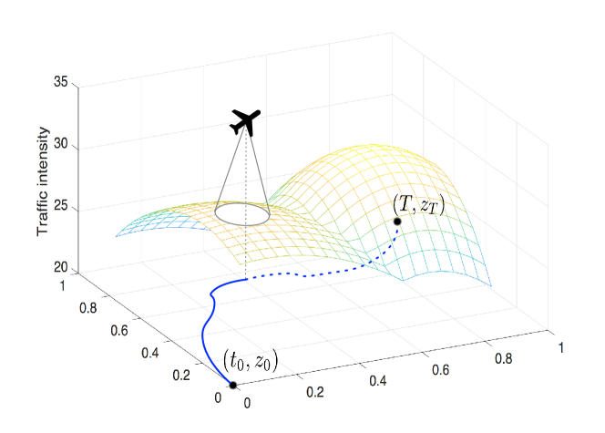
Figure 1: A UAV Base Station travels from $z_{0}$ at $t_{0}$ to $z_{T}$ at $T$ and serves a user traffic characterized by its intensity.

We consider a network area characterized by a traffic density at position $z$ and time $t$. We intend to control the trajectory and the velocity of a UAV base station, which is located in $z_{0}\triangleq z(t_{0})$ at $t_{0}$ and shall reach a destination $z_{T}\triangleq z(T)$ at $T$ with the aim of minimizing a cost determined by the velocity and the traffic, defined hereafter by (2). At $(t,z)$, we assume that the UAV BS is able to cover an area, from which it can serve users (see Figure 1). The velocity of the UAV BS induces an energy cost. In this model, we control the velocity vector $a$ of the UAV BS. The general form of the cost function is as follows

$$\mathcal{L}(t,z,a)=\frac{K}{2}||a||^{2}-u(t,z)$$ (2)

where the first term is a cost related to the velocity of the vehicle ($K$ is a positive constant), and $\|\cdot\|$ denotes the usual Euclidean norm. The higher is the speed, the higher is the energy cost. The second term is a user traffic intensity, i.e., the amount of traffic served by the UAV BS at $(t,z)$. Note that a non-zero energy at null speed can be incorporated in the model by adding a constant. Without loss of generality, we assume that this constant is null.

Let $S(t_{0},z_{0},T,z_{T})$ be the minimal total cost along any trajectory between $z_{0}$ at $t_{0}$ and $z_{T}$ at $T$ (also called the action in mechanics or value function in control theory). Let us define $\Omega(t_{0},T)$ as the space of absolutely continuous functions from $[t_{0};T]$ to $\mathbb{R}^{2}$. Our problem can now be formulated as follows

$$S(t_{0},z_{0},T,z_{T})\!\!\! \!=\!\!\!\! \!\!\!\!\!\min_{a\in\Omega(t_{0},T)}\!\!\int_{t_{0}}^{T}\!\!\!\!\mathcal{L}(s,z(s),a(s))ds\!\!+\!\!J(z(T))$$ (3)

where $\frac{dz}{dt}(t)=a(t)$, $z(t_{0})=z_{0}$, and $J$ is the terminal cost defined by $J(z)=0$ if $z=z_{T}$ and $J(z)=+\infty$ otherwise. For simplicity reasons, we assume the existence and uniqueness of the optimal control $a^{*}(t)$ in (3) and denote the associated optimal trajectory $z^{*}(t)$. In a traffic map symmetric with respect to $z_{0}$ and $z_{T}$, the reader can convince himself that the uniqueness is not guaranteed.

II-B Preliminary Results From Lagrangian Mechanics

We provide in this section important results from the Lagrangian mechanics for the convenience of the reader.

Definition 1 (Impulsion).

The impulsion function is defined as

$$p(t,z,a):=\nabla_{a}\mathcal{L}(t,z,a).$$ (4)

In the Newtonian classical framework that is used here (see (2)), the impulsion is the product of the particle mass by its velocity (hence the standard term “impulsion”).

Definition 2.

The Hamiltonian function is defined as

$$H(t,z,p):=\max_{a\in\mathbb{R}^{2}}p\cdot a-\mathcal{L}(t,z,a).$$ (5)

Lemma 1 (Euler-Lagrange Equations).

Along the optimal trajectory $z^{*}(t)$ that starts from $z_{0}$ at $t_{0}$ and ends at $z_{T}$ at $T$, we have

$$\frac{d}{dt}\nabla_{a}\mathcal{L}(t,z^{*}(t),a^{*}(t))=\nabla_{z}\mathcal{L}(t,z^{*}(t),a^{*}(t))$$ (6)

or equivalently

$$\frac{dp}{dt}(t,z^{*}(t),a^{*}(t))=\nabla_{z}\mathcal{L}(t,z^{*}(t),a^{*}(t)).$$ (7)

Proof.

See Appendix -A. ∎

The Euler-Lagrange equation is the first-order necessary condition for optimality and holds for every point on the optimal trajectory.

Lemma 2.

If the Lagrangian $\mathcal{L}(t,z,a)$ is time-independent and $\alpha$-homogeneous in $z$ and $a$ for $\alpha>0$, i.e., $\mathcal{L}(\lambda z,\lambda a)=|\lambda|^{\alpha}\mathcal{L}(z,a)$ for all $\lambda\in\mathbb{R}$, $S$ given by (3) reads

$$S(t_{0},z_{0},T,z_{T})=\frac{1}{\alpha}[z\cdot p]_{t_{0}}^{T}+J(z_{T}).$$ (8)

Proof.

See Appendix -B. ∎

Lemma 3 (Hamilton-Jacobi).

Along the optimal trajectory, we have for $t\in(t_{0};T)$ using previous notations

$$\dfrac{\partial{S}}{\partial{T_{1}}}(t,z^{*}(t),T,z_{T})=H(t,z^{*}(t),-p^{*}(t)),$$ (9)

$$\dfrac{\partial{S}}{\partial{T_{2}}}(t_{0},z_{0},t,z^{*}(t))=-H(t,z^{*}(t),p^{*}(t)),$$ (10)

where

$$p^{*}(t)=\nabla_{a}\mathcal{L}(t,z^{*}(t),a^{*}(t))=\nabla_{X_{1}}S(t_{,}z^{*}(t),T,z_{T}).$$ (11)

Proof.

See Appendix -C. ∎

From now, we assume that the Lagrangian is time-independent, i.e., $\mathcal{L}(t,z,a)=\mathcal{L}(z,a)$, and is an even function in $a$, i.e., $\mathcal{L}(z,-a)=\mathcal{L}(z,a)$. A direct consequence is that $H$ is time-independent and is an even function in $p$, i.e., we write $H(t,z,p)=H(z,p)$ and $H(z,-p)=H(z,p)$.

III Optimal Trajectory

In this section, we characterize the optimal trajectory when the traffic intensity is a quadratic form and also when it is made of two regions of quadratic form separated by an interface. We call these two cases single-phase and bi-phase intensities respectively. Both cases satisfy our assumptions on the Lagrangian with $\alpha=2$.

III-A Single-Phase Optimal Trajectory

Assume that the traffic intensity is of the form $u(z)=\frac{1}{2}u_{0}||z||^{2}$. When $u_{0}>0$, this function models a traffic hole in $z=0$. When $u_{0}<0$, it models a traffic hot spot at $z=0$. We disregard the case $u_{0}=0$ because it corresponds to a constant traffic intensity that is not of interest in this paper. Thus the cost function has the following form

$$\mathcal{L}(z,a)=\frac{1}{2}K||a||^{2}-\frac{1}{2}u_{0}||z||^{2}.$$ (12)

Note that

$$p(z,a)=\nabla_{a}\mathcal{L}(z,a)=Ka.$$ (13)

III-A1 Trajectory Equation

In the single phase case, we have a closed form expression of the trajectory.

Theorem 1.

If $u_{0}<0$, the cost function is given by (14),

$$S(t_{0},z_{0},T,z_{T})=\frac{K\omega}{2\sinh\omega(T-t_{0})}\left((|z_{0}|^{2}+|z_{T}|^{2})\cosh\omega(T-t_{0})-2z_{0}\cdot z_{T}\right)+J(z_{T})$$ (14)

the optimal trajectory is

$$z^{*}(t)=\frac{z_{T}\sinh(\omega(t-t_{0}))+z_{0}\sinh(\omega(T-t))}{\sinh(\omega(T-t_{0}))}$$ (15)

and the control is given by

$$a^{*}(t)=\omega\frac{z_{T}\cosh(\omega(t-T))-z_{0}\cosh(\omega(T-t))}{\sinh(\omega(T-t_{0}))}$$ (16)

where $\omega^{2}=-\frac{u_{0}}{K}$.
If $u_{0}>0$, the cost function is given by (17),

$$S(t_{0},z_{0},T,z_{T})=\frac{K\omega}{2\sin\omega(T-t_{0})}\left((|z_{0}|^{2}+|z_{T}|^{2})\cos\omega(T-t_{0})-2z_{0}\cdot z_{T}\right)+J(z_{T})$$ (17)

the optimal trajectory is

$$z^{*}(t)=\frac{z_{T}\sin(\omega(t-t_{0}))+z_{0}\sin(\omega(T-t))}{\sin(\omega(T-t_{0}))}$$ (18)

and the control is given by

$$a^{*}(t)=\omega\frac{z_{T}\cos(\omega(t-t_{0}))-z_{0}\cos(\omega(T-t))}{\sin(\omega(T-t_{0}))}$$ (19)

where $\omega^{2}=\frac{u_{0}}{K}$.

Proof.

See Appendix -D. ∎

Corollary 1.

If the user traffic intensity is of the form $u(t,z)=\frac{1}{2}u_{0}||z||^{2}+u_{0}z\cdot e+u_{1}$ with $u_{1}\in\mathbb{R}$ and $e\in\mathbb{R}^{2}$, then define $\tilde{z}=z+e$, $\tilde{z}_{0}=z_{0}+e$, $\tilde{z}_{T}=z_{T}+e$ and trajectories given in Theorem 1 are valid by replacing $z$, $z_{0}$, $z_{T}$ by $\tilde{z}$, $\tilde{z}_{0}$, $\tilde{z}_{T}$, respectively. The cost function becomes: $S(t_{0},z_{0},T,z_{T})=\frac{1}{\alpha}[z\cdot p]_{t_{0}}^{T}+J(z_{T})-u_{1}(T-t_{0})$.

Corollary 2.

If the user traffic intensity is of the form $u(t,z)=\sum_{i}u_{i}||z-z_{i}||^{2}$ with $\sum_{i}u_{i}\neq 0$, then $u(t,z)=(\sum_{i}u_{i})||z-z_{b}||^{2}+\sum_{i}u_{i}||z_{i}-z_{b}||^{2}$ with $z_{b}=\frac{\sum_{i}u_{i}z_{i}}{\sum_{i}u_{i}}$. Define $\tilde{z}=z+z_{b}$, $\tilde{z}_{0}=z_{0}+z_{b}$, $\tilde{z}_{T}=z_{T}+z_{b}$, $\tilde{u}_{0}=\sum_{i}u_{i}$ and trajectories given in Theorem 1 are valid by replacing $z$, $z_{0}$, $z_{T}$, $u_{0}$ by $\tilde{z}$, $\tilde{z}_{0}$, $\tilde{z}_{T}$, $\tilde{u}_{0}$ respectively.

The system is thus equivalent to the one assumed in Theorem 1 by changing the origin of the locations to the barycentre $z_{b}$ of the $z_{i}$.

III-A2 Traffic Hot Spot, Traffic Hole

We assume that there is a hot spot or a traffic hole located in $z_{h}$ and that the traffic intensity is of the form $u(t,z)=\frac{1}{2}u_{0}||z-z_{h}||^{2}+u_{1}=\frac{1}{2}u_{0}||z||^{2}-u_{0}z\cdot z_{h}+\frac{1}{2}u_{0}||z_{h}||^{2}+u_{1}$. We can apply Corollary 1 with $e=-z_{h}$. Figure 2 shows optimal trajectories when $z_{h}$ is a hot spot, i.e., for $u_{0}<0$, and different values of $K$. The starting point is $z_{0}$ and the destination is $z_{T}$. When $K$ increases, the velocity cost increases and the trajectories tend to the straight line between $z_{0}$ and $z_{T}$, which minimizes the speed. When $K$ is small, the UAV can go fast to $z_{h}$, reduces its speed in the vicinity of the hot spot and then goes fast to the destination (in order to decrease the cost function (2) by increasing its traffic contribution).

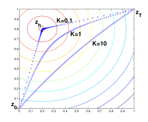
Figure 2: Traffic hot spot ($u_{0}<0$). Circles are iso-traffic levels.

Figure 3 shows optimal trajectories when $z_{h}$ is a traffic hole, i.e., for $u_{0}>0$. In Figure 3(a), $T$ is smaller than the period of the ellipse, i.e., $\frac{2\pi}{\omega}>T$. When $K$ decreases, the UAV can spend more time in the areas of higher traffic intensity. In Figure 3(b), $T$ is larger than the period. In this case, the trajectory follows one period of the ellipse whose equation is given by (18) plus a part of the same ellipse from $z_{0}$ to $z_{T}$.

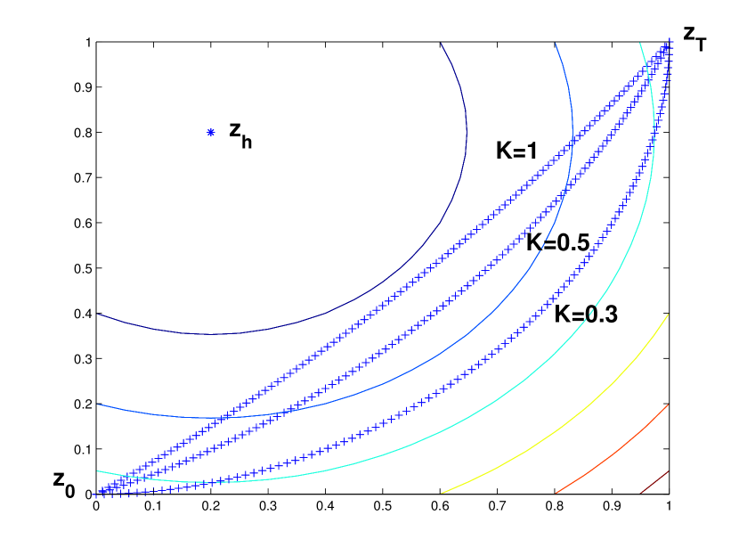
(a) $T$ is smaller than the ellipse period.

(b) $T$ is larger than the ellipse period.

Figure 3: Traffic hole ($u_{0}>0$). Circles are iso-traffic levels.

III-B Multi-Phase Trajectory Characterization

We now consider a traffic intensity (or potential) consisting in two quadratic functions separated by an interface $\mathcal{I}$ of equal potentials delimiting two regions $1$ and $2$. The interface is defined by an equation $f(z)=C$, where $C$ is a constant and $f$ is a differentiable function. We assume that the optimal trajectory crosses the interface only once, at position $\xi$ and time $\tau$. The impulsion $p^{*}$ is defined everywhere on the optimal trajectory between $(t_{0},z_{0})$ and $(T,z_{T})$. The following notations will be used in the sequel:

$$p^{-}=p^{*}(\tau^{-})=\lim\limits_{\begin{subarray}{c}s\to\tau\\ s<\tau\end{subarray}}\ p^{*}(s)\enspace,\ p^{+}=p^{*}(\tau^{+})=\lim\limits_{\begin{subarray}{c}s\to\tau\\ s>\tau\end{subarray}}\ p^{*}(s)\enspace,\ H^{-}=H_{1}(\xi,p^{*}(\tau^{-}))\enspace,\ H^{+}=H_{2}(\xi,p^{*}(\tau^{+})).$$ (20)

Theorem 2.

The location and time $(\xi,\tau)$ of interface crossing are characterized by the following equations

$$p^{-}-p^{+}-\mu\ \nabla_{z}f(\xi) = 0$$ (21)

$$H^{+}-H^{-} = 0$$ (22)

$$f(\xi) = C$$ (23)

for some Lagrange multiplier $\mu\in\mathbb{R}$

Proof.

See Appendix -E. ∎

Equation (22) expresses the fact the energy is conserved when crossing the interface. One can show that actually the energy is conserved along the whole trajectory. Equation (21) is related to the conservation of the tangential component of the impulsion at the interface. Equation (23) is the interface equation at $\xi$. One can show that under the assumption of equal potential on the interface, the kinetic energy, the impulsion, and the velocity vector are conserved across the interface.

III-C Multi-phase optimal trajectory uniqueness and value function convexity issues

Looking for uniqueness/non-uniqueness of optimal multi-phase trajectories leads naturally to study the convexity of the multi-phase total cost. As stated in Appendix -E this cost is additive and satisfies the dynamic programming principle which reads

$$\bar{S}(\Theta=\tau,\ \Xi=\xi\ |\ t_{0},z_{0},T,z_{T})=S_{1}(t_{0},z_{0},\tau,\xi)+S_{2}(\tau,\xi,T,z_{T})$$ (24)

where $S_{1}$ and $S_{2}$ are themselves minimal. Hamilton-Jacobi equations applied to each cost component allows to study their first- an second- order differential properties such as convexity. For instance in the chosen quadratic model, each single-phase (minimal) total cost $S_{1}(t_{0},z_{0},\tau,\xi)$, $S_{2}(\tau,\xi,T,z_{T})$ given by Corollary 1 and (14) is convex (since it is a positive quadratic form with respect to the spatial coordinates) with respect to the spatial position $\xi$, but not necessarily so with respect to the interface crossing time $\tau$. We consider in what follows a general form of the single-phase value function between $(t_{1},x_{1})$ and $(t_{2},x_{2})$ that is denoted by

$$S(t_{1},x_{1},t_{2},x_{2}).$$

We also note by $\omega$ the pulsation, $\phi=\omega\ (t_{2}-t_{1})$ is the temporal phase and ${p}_{1},\ {p}_{2}$ are the the initial and final impulsions as derived from formula (16).

Theorem 3.

i) The Hessian of the single-phase cost wrt.  any joint variable $\psi_{i}=$ ${(T_{i},X_{i})}_{i=1,2}$  is

$${\cal H}(\psi_{i})=\nabla^{2}_{T_{i},X_{i}}\ S(t_{1},x_{1},t_{2},x_{2}) =\left(\begin{array}[]{l | c}\alpha&\hskip 5.69054pt{\Pi_{i}}^{\dagger}\\[2.84526pt] \hline\cr\Pi_{i}&\hskip 11.38109ptKg\ \mbox{Id}_{2}\end{array}\right)\hskip 2.84526pt\mbox{ with }\hskip 2.84526pt\left\{\begin{array}[]{l}\alpha=\dfrac{\partial^{2}S}{\partial T_{i}^{2}}=\dfrac{\omega\ {p}_{1}\cdot{p}_{2}}{K\ \sinh\phi}\\[11.38109pt] g=\omega\ \coth\phi\ >0\\[11.38109pt] \Pi_{i}=-\dfrac{\omega\ p_{3-i}}{\sinh\phi}\in\mathbb{R}^{2}\end{array}\right.$$ (30)

where $p_{i}$ is the impulsion at time $T_{i}$, i.e., at extremity $X_{i}$  ($i=1,2$ and $j=3-i$).
ii) At most one eigenvalue of ${\cal H}(\psi_{i})$ can be negative and $\alpha<0$ is a sufficient condition for this to hold, namely implying local non-convexity of the (single-phase) value function.
iii) The double-phase Hessian enjoys a similar structure as (30) and writes with respect to the variable $\Psi=(\Theta,\Xi)$

$$\bar{{\cal H}}(\Theta=\tau,\Xi=\xi)= \ {\cal H}_{1}(\chi_{2})+{\cal H}_{2}(\chi_{1})=\left(\begin{array}[]{l | c}\alpha&\hskip 5.69054pt{\Pi}^{\dagger}\\[2.84526pt] \hline\cr\Pi&\hskip 11.38109ptKh\ \mbox{Id}_{2}\end{array}\right)$$ (31c)

with $$\left\{\begin{array}[]{l}\alpha=\dfrac{\partial^{2}{S_{1}}}{\partial{T_{2}}^{2}}(t_{0},z_{0},\tau,\xi)+\dfrac{\partial^{2}{S_{2}}}{\partial{T_{1}}^{2}}(\tau,\xi,T,z_{T})\ \ (\mbox{cf. }\eqref{full-single-phase-hessian:eq})\\[11.38109pt] h=\omega_{1}\ \coth\phi_{1}+\omega_{2}\ \coth\phi_{2}\\[11.38109pt] \Pi=-\left[\dfrac{\omega_{1}\ p(t_{0})}{\sinh\phi_{1}}+\dfrac{\omega_{2}\ p(T)}{\sinh\phi_{2}}\right]\\[11.38109pt] \mbox{and }\phi_{1}=\omega_{1}\ (\tau-t_{0}),\ \phi_{2}=\omega_{2}\ (T-\tau)\end{array}\right.$$ (31h)

and may thus be non-convex as well.

Proof.

See Appendix -F subsections -F1 and -F2. ∎

In the single-phase case, the sufficient condition ii) i.e., $\alpha<0$, supports first a physical interpretation (see Fig. 4) and also a geometrical one (see next Theorem 4 and Fig. 5).

Figure 4: Physical interpretation of local convexity vs. non-convexity of the single-phase cost:
the initial and final impulsions $({p}_{1},{p}_{2})$ form an obtuse angle $\Rightarrow$ the value function is non-convex.

Theorem 4.

Let $u=\frac{x_{1}+x_{2}}{2}$ and $v=\frac{x_{2}-x_{1}}{2}$. (Note that $\|u\|$ is the distance from the hotspot to the average of $x_{1}$ and $x_{2}$, and the $\|v\|$ is the half-distance between $x_{1}$ and $x_{2}$.) Then the following sufficient condition holds

$$\dfrac{\parallel v\parallel}{\parallel u\parallel}<\dfrac{\cosh\phi-1}{1+\cosh\phi}=\tanh^{2}\dfrac{\phi}{2}\Rightarrow\alpha=\dfrac{\partial^{2}{S}}{\partial{t_{i}}^{2}}<0.$$

Proof: We combine the formulas (63) and (64) in (68) to obtain

$$\alpha=\dfrac{w}{K}\ \dfrac{{p}_{1}\cdot{p}_{2}}{\sinh\phi}=\dfrac{K\,\omega^{3}}{\sinh^{3}\phi}\left[(\parallel{x}_{1}\parallel^{2}+\parallel{x}_{2}\parallel^{2})\ \cosh\phi-{x}_{1}\ .\ {x}_{2}\ (1+\cosh^{2}\phi)\right]$$ (32)

which can be rewritten as

$$\alpha=\dfrac{K\,\omega^{3}}{\sinh^{3}\phi}\left[-\parallel u\parallel^{2}\ (1-\cosh\phi)^{2}+\parallel v\parallel^{2}\ (1+\cosh\phi)^{2})\right].\hfill\qed$$

This non-convexity condition for the single-phase value function interprets as: long phase ($\tanh\frac{\phi}{2}>\frac{1}{2}$) and long distances between the hotspot $z_{h}$ to both initial and final positions ${x}_{1}$, ${x}_{2}$, relatively to their mutual distance ($\frac{\parallel u\parallel}{\parallel v\parallel}\ggg 1$).

Figure 5: Geometrical interpretation of local non-convexity: long time and long distance to the hotspot.

Several preliminary simulations show that when this case happens for two phases, the total value function is indeed non-convex and that several (local) optimal solutions may indeed exist.

IV Algorithms

Previous propositions allow us to propose several numerical algorithms seeking optimal trajectories. In this section, we present two algorithms aiming this goal: a gradient descent algorithm and a bisection search method based on the linear control property (16).

IV-A A Gradient Descent Algorithm Grad-Algo

In this section, we propose Grad-Algo (Algorithm 1) which is an alternated optimization-based algorithm relying on the following procedures.

Procedure for seeking an optimal $\xi$ given a fixed $\tau$

from Hamilton-Jacobi equations (Lemma 3 and Appendix -C) the gradient of the total cost function with respect to $\xi$ is $p^{*}(\tau^{-})-p^{*}(\tau+)$. Equation (13) says that in the Newtonian framework the impulsion is proportional to the control variable $a$. Equation  (16) says that in the quadratic model the velocity vector is, at any time a linear combination of centered initial and final positions. Then the searched gradient appears to be an affine function of $\xi$ which reads

$$p^{*}(\tau^{-})-p^{*}(\tau+) =\nabla_{X_{2}}S_{1}(t_{0},z_{0},\tau,\xi)+\nabla_{X_{1}}S_{2}(\tau,\xi,T,z_{T})\$$

$$=Kh\ (\xi-B).$$ (33)

Scalar $h$ and point $B$ (where the spatial gradient cancels at fixed $\tau$ i.e.,  $p^{*}(\tau^{-})=p^{*}(\tau+)$) verify

$$h = \omega_{1}\,\coth(\omega_{1}(\tau-t_{0}))+\omega_{2}\,\coth(\omega_{2}(T-\tau)),$$ (34)

$$B = \dfrac{1}{h}\big{[}\ \omega_{1}\,z_{h1}\,\coth(\omega_{1}(\tau-t_{0}))+\omega_{2}\,z_{h2}\,\coth(\omega_{2}(T-\tau))$$ (35)

$$+\dfrac{\omega_{1}\,(z_{0}-z_{h1})}{\sinh(\omega_{1}(\tau-t_{0}))}+\dfrac{\omega_{2}\,(z_{T}-z_{h2})}{\sinh(\omega_{2}(T-\tau))}\ \big{]}.$$

The equation involving the Lagrange multiplier (21) now reads

$$Kh\ (\xi-B)-\mu\ \nabla_{\xi}f(\xi)=0$$ (36)

and shows that the optimal location $\xi^{*}$ is the orthogonal projection of $B$ on the interface ${\cal I}$.

Procedure for seeking an optimal $\tau$ given a fixed $\xi$

we use the result of Theorem 2. As also shown by Hamilton-Jacobi equations (Lemma 3 and Appendix -C), the gradient of $S$ with respect to $\tau$ is given by $H_{2}(\xi,p^{*}(\tau^{+}))-H_{1}(\xi,p^{*}(\tau^{-}))$. The Hamiltonians are easily computed in each phase by applying the classical Newton formula at given location $(z,t)$

$$H(p,z,t)=\dfrac{{\parallel{p}\parallel}^{2}}{2\ K}+V(z).$$

We then update $\tau$ by using a simple gradient descent scheme (see Algorithm 1).

Stop criteria

the search procedure is performed until the impulsion and the Hamiltonian have converged with a given accuracy. For this purpose we consider the function $g:(\mathbb{R}^{n}\setminus\{0\})\times(\mathbb{R}^{n}\setminus\{0\})\mapsto\mathbb{R}$
defined as follows $g(x,y)=\dfrac{\parallel{x-y}\parallel}{\inf(\parallel{x}\parallel,\parallel{y}\parallel)}\ \ \ \mbox{ which measures a relative ``discrepancy" between $x$ and $y$}.$ Now let us give $\epsilon_{p}$ and $\epsilon_{H}$ (typically of the order of $2.10^{-4}$) and define the stop criteria as follows

$$\texttt{STOP}=g(p^{+},p^{-})~{}/~{}\epsilon_{p}<1\ \ \ \&\&\ \ g(H^{+},H^{-})~{}/~{}\epsilon_{H}<1.$$ (37)

Algorithm 1 Grad-Algo An uncoupled projected gradient descent algorithm

1:Input: precisions $\epsilon_{p}$, $\epsilon_{H}$ ($\epsilon_{p}=\epsilon_{H}$ = $2.10^{-4}$), $M_{\tau}=$ number of gradient descent iterations on $\tau$

2:Init: starting position $\xi\leftarrow$ $\xi_{0}$ e.g., = $\frac{z_{0}+z}{2}$ , $\tau\leftarrow$ $\tau_{0}$ e.g., = $\frac{t_{0}+T}{2}$

3:Output: $(\tau,\xi)$

4:procedure TWO_PHASE($\tau,\xi$)

5:     computes: the current bi-phase trajectory given by $(t_{0},z_{0})\rightarrow(\tau,\xi)\rightarrow(T,z_{T})$

6:     return $(B,H^{+},H^{-},\bar{\cal H})$ = (the B-point (35), the two phase Hamiltonians and the total Hessian at current location $(\tau,\xi)$  (24, 31c, 31h))

7:end procedure

8:$N_{step}=0$

9:$(B,H^{+},H^{-},{\bar{\cal H}})=\texttt{TWO\_PHASE}({\tau,\xi})$

10:repeat

11:     $\xi\leftarrow\mbox{Proj}_{{\cal I}}(B)$ (36)

12:     for $m=1,\dots,M_{\tau}$ do

13:         $\tau\leftarrow\tau-\dfrac{(H^{+}-H^{-})}{\alpha}$  with $\alpha={\bar{\cal H}}_{11}=\dfrac{\partial^{2}{\bar{S}}}{\partial\Theta^{2}}(\tau,\xi)$  (Newton descent wrt.  $\tau$)

14:         $(B,H^{+},H^{-},{\bar{\cal H}})=\texttt{TWO\_PHASE}({\tau,\xi})$

15:     end for

16:     $N_{step}=N_{step}+1$

17:until STOP (37)

Complexity: Algorithm 1: if $\alpha^{*}=\dfrac{\partial^{2}{\bar{S}}}{\partial{\Theta}^{2}}(\tau^{*},\xi*)\neq 0$ then the convergence of Newton descent on $\tau$ is quadratic (see [35] for instance). If $\alpha^{*}=0$ say, $H_{2}(\xi,p^{*}(\tau^{+}))-H_{1}(\xi,p^{*}(\tau^{-}))\sim(\tau-\tau^{*})^{\nu}$ with $\nu\geq 2$, the convergence is linear (see [35] for instance). For safety we take $M_{\tau}=10$ i.e., $\nu\approx 2$. The global complexity is $O(N_{step}\ M_{\tau})$ and usually $N_{step}=2$.

IV-B The B-curve algorithm B-Algo

The $B$-curve algorithm aims to overcome the non-convexity issues developed previously. It proceeds as follows. Consider the $B$ point defined in formula (35). We notice that for each $\tau\in[t_{0},T]$ this point is defined univocally knowing all parameters ($t_{0},\ T,\ z_{0},\ z_{T},\ z_{h}$) and all (quadratic) traffic profiles so that we can see $B$ in (35) as a function of $\tau$, denoted $B(\tau)$. It can be shown that this function $\tau\mapsto B(\tau)$ is continuous in the interval $[t_{0},T]$ and that $\lim_{\tau\rightarrow t_{0}^{+}}{B(\tau)}=z_{0}$, $\lim_{\tau\rightarrow T^{-}}B(\tau)=z_{T}$. Assume now that the two optimal sub-trajectories are such that crossing time $\tau\in[t_{0},T]$ and interface position $\xi$ verify $\xi=B(\tau)$. Then by formula (33) the spatial gradient of $S$ at point $\xi$ is

$$p^{*}(\tau^{-})-p^{*}(\tau+)=0$$ (38)

This implies that the kinetic components of both Hamiltonians are equal at the interface. Now since $\xi$ belongs to the interface, both phase potentials (traffics) are equal by definition, so that the total Hamiltonian is also conserved at the interface: this is the optimality condition required with respect to time $\tau$. To summarize, in these conditions, both the Hamiltonian and the total impulsion are conserved at interface $\mathcal{I}$, i.e., local optimality conditions hold for the total value function. It is also worth noticing that the related Lagrange multiplier appearing in (36) now simply vanishes: $\mu=0$. The proposed B-algorithm consists then in seeking the intersection of the B-curve ${\cal B}=\{B(\tau),\tau\in[t_{0},T]\}$ with the interface ${\cal I}$ (Algorithm 2). For this, we first select precision $\epsilon_{B}$, then proceed by bisection and check the stopping criterion

$$\texttt{STOP}\_\texttt{B}=\dfrac{|{t_{2}-t_{1}}|}{|{b-a}|}\ \dfrac{1}{\epsilon_{B}}\ \ \ <1.$$ (39)

Complexity: Algorithm 2: if $\epsilon_{B}=\dfrac{1}{2^{m}}$ then the bisection algorithm converges in $m$ iterations. Its complexity is thus $O(\log\dfrac{1}{\epsilon_{B}})$. In our experiments we chose $\epsilon_{B}=2.10^{-4}$ $\approx\dfrac{1}{2^{12}}$ and 12 iterations are indeed sufficient to provide a trajectory with optimality conditions holding at this (relative) precision.

Algorithm 2 the B-curve bisection algorithm

Input: initial/final time search interval $[a,b]\in[t_{0},T]$, precision $\epsilon_{B}$ fixed by the user ($\epsilon_{B}=2.10^{-4}$)

Output: $(\xi,\tau)$

Init: $t_{1}\leftarrow a\enspace,t_{2}\leftarrow b$, the algorithm only starts if IN_ZONE2($B(a)$) $\neq$ IN_ZONE2($B(b)$)

procedure IN_ZONE2($z$)

     $u_{i}(z)$ = (time-stationary) traffic $u(z)$ from hotspot $z_{hi}$ at point $z$  ($i=1,2$)

     return $(u_{2}(z)>u_{1}(z))$

end procedure

repeat

     $x_{1}\leftarrow B(t_{1})$  , $x_{2}\leftarrow B(t_{2})$

     $\tau\leftarrow\dfrac{t_{1}+t_{2}}{2}\enspace,\ \xi\leftarrow B(\tau)$

     if (IN_ZONE2($\xi$) == IN_ZONE2($x_{2}$)) then

         $t_{2}\leftarrow\tau$

     else  $t_{1}\leftarrow\tau$

     end if

     compute stop criterion STOP_B  (39)

until STOP_B

$\xi\leftarrow B(\tau)$

V Numerical Experiments

V-A From Measurements to Quadratic Profile

In this section, we explain how from measured or estimated traffic load, we can derive a quadratic model that will allow us to apply our framework. To illustrate the procedure, we extract data from the open data set presented in [34]. Traffic data (in number of bytes) has been collected from an operational cellular network in a medium-size city in China and is recorded for every base station and every hour. For our experiment, we extract a rectangle region $[X_{\min},X_{\max}]\times[Y_{\min},Y_{\max}]$, where $X_{\min}=111$, $X_{\max}=111.12$, $Y_{\min}=13.12$, $Y_{\max}=13.22$ are the minimum and maximum longitude and latitude respectively (real figures have been anonymized). This corresponds approximately to a rectangle of $11$ km$\times 13$ km with $400$ base stations having an average cell range of $337$ m. The traffic of the 22th August 2012 between 5 and 6pm is illustrated in Figure 6(a). We assume that this traffic is representative of the traffic intensity when the drone is launched. In order to fit this raw data to our model, we follow the pre-processing steps shown in Algorithm 3.

Algorithm 3 Data preprocessing

1:First smoothing: data aggregation

2:Second smoothing: LOWESS

3:Normalization

4:K-means with quadratic models

The first smoothing consists in aggregating the traffic data on a grid of $50$ steps in both longitude and latitude directions. The resulting elementary regions should correspond approximately to the drone coverage. The result is shown in Figure 6(b). The data exhibits a very high variability with very high peaks around few locations. The second smoothing is a Locally Weighted Scatterplot Smoothing (LOWESS) [36]. We use here the Matlab function fit with the option ”Lowess”. The choice of the smoothing parameter $\alpha$, i.e., the proportion of data points used for every local regression, has a decisive impact on the result. Increasing $\alpha$ has the effect of averaging out the different peaks. In our specific scenario, $\alpha=0.25$ yields Figure 7(a) with two local maxima. With $\alpha=0.5$, we obtain a single maximum. In step 3 of the pre-processing, the traffic is normalized between $0$ and $1$ with no influence on the optimal trajectory.

The final pre-processing step is an adaptation of the classical K-means algorithm (see Algorithm 4) to fit to quadratic models. Inputs are the data points obtained after the normalization, $K_{c}$, the number of clusters (or hot spots), $K_{n}$ the number of nearest neighbors and $M$ the number of iterations. Every cluster is associated to a quadratic function (in our case, we have $K_{c}=2$). Every data point $j$ is associated to a cluster and has a related label $L_{j}$ in $\{1,...,K\}$. For every data point, a list of nearest neighbors is built (step 4). An arbitrary initial labelization is chosen (step 6). The algorithm then proceeds by iterations (steps 7-16). At every iteration, if a point $j$ has some neighbor with a different label (step 9), a best new label is found for $j$ (step 10-13) in terms of quadratic error $e_{k}$. The error $e_{k}$ measures the difference between the data points and the $K_{c}$-quadratic model, which fits a quadratic function to every cluster assuming that $j$ has label $k$ (steps 18-31). In Algorithm 4, $\texttt{KNN}(K_{n},X,Y)$ is a procedure that finds the $K_{n}$ nearest neighbors of $(X,Y)$ with respect to the Euclidian distance. We use the Matlab implementation knnsearch. $\texttt{NLLS}(\mathcal{L})$ is a non-linear least square method that fits data points in $\mathcal{L}$ to a quadratic function of the form $\frac{1}{2}u_{0}|z-z_{h}|^{2}+u_{1}$. The Matlab implementation is based on a trust-region approach of the Levenberg-Marquardt Algorithm.

Algorithm 4 K-means with quadratic models

1:Input: $K_{c}$ (number of clusters), $J$ (number of measurement points) $(X_{j},Y_{j},Z_{j})$, $j=1,\dots,J$ (coordinates and estimated traffic load $Z_{j}$ in $(X_{j},Y_{j})$), $K_{n}$ (number of nearest neighbors), $M$ (number of iterations)

2:Output: $z_{hk}$, $u_{0k}$, $u_{1k}$ $k=1,\dots,K_{c}$ (hot spot characteristics), $e$ (quadratic error)

3:for $j=1,\dots,J$ do

4:     $\mathcal{K}_{j}\leftarrow\texttt{KNN}(K_{n},X_{j},Y_{j})$

5:end for

6:$L\leftarrow$ Initial labelization

7:for $m=1,\dots,M$ do

8:     for $j=1,\dots,J$ do

9:         if $\exists j^{\prime}\in\mathcal{K}_{j}$ s.t. $L_{j^{\prime}}\neq L_{j}$ then

10:              for $k=1...K_{c}$ do

11:                  $e_{k},z_{hl},u_{0l},u_{1l}$, $l=1,\dots,K_{c}$ $\leftarrow\texttt{FIT}((X,Y,Z),j,L,k,K_{c})$

12:              end for

13:              $L_{j}\leftarrow\arg\min_{k}e_{k}$

14:         end if

15:     end for

16:end for

17:return $z_{hk}$, $u_{0k}$, $u_{1k}$ $k=1,\dots,K_{c}$, global quadratic error

18:procedure FIT($(X,Y,Z)$, $j$,$L$,$k$,$K_{c}$)

19:     $L_{j}\leftarrow k$

20:     for $l=1$,…,$K_{c}$ do

21:         $\mathcal{L}_{l}\leftarrow\{(X_{i},Y_{i},Z_{i})|L_{i}=l\}$

22:         $z_{hl},u_{0l},u_{1l}\leftarrow\texttt{NLLS}(\mathcal{L}_{l})$

23:     end for

24:     $e_{k}\leftarrow 0$

25:     for $j=1$,…,$J$ do

26:         $\tilde{Z}_{j}\leftarrow\max_{l=1,\dots,K_{c}}\frac{1}{2}u_{0l}|z-z_{hl}|^{2}+u_{1l}$

27:         $e_{k}\leftarrow e_{k}+|\tilde{Z}_{j}-Z_{j}|^{2}$

28:     end for

29:     $e_{k}\leftarrow e_{k}/J$

30:     return $e_{k},z_{hl},u_{0l},u_{1l}$, $l=1,\dots,K_{c}$

31:end procedure

Complexity: Algorithm 4: Searching the $K_{n}$-nearest neighbors of a data point using k-d trees takes $O(K_{n}\log J)$ in average and $O(K_{n}J)$ in the worst case. Steps 3-5 has thus a complexity of $O(K_{n}J\log J)$ in average and $O(K_{n}J^{2})$ in the worst case. Initial labelization is a simple linear partitioning of the 2D space in $K_{c}$ zones and is thus performed in $O(J)$. In the main loop, there are at most $O(MJK_{c})$ calls to the function FIT. The Levenberg-Marquardt Algorithm requires $O(\epsilon^{-2})$ iterations to reach an $\epsilon$-approximation of a stationary point of the objective function [37, 35]. The overall complexity of Algorithm 4 is thus $O(K_{n}J^{2}+MJK\epsilon^{-2})$.

The K-means partition obtained after $M=12$ iterations is shown in Figure 7(b). The final fits are shown in Figures 9(a) and 9(b) for $(K_{c},\alpha)=(2,0.25)$ and $(K_{c},\alpha)=(1,0.5)$, respectively. Figure 8 shows the quadratic error as a function of the number of iterations of the K-means algorithm for $K_{c}=1$ and $K_{c}=2$. The error is constant for $K_{c}=1$ as there is only one iteration, which performs the non-linear least square fitting for the single cluster. For $K_{c}=2$, we distinguish two cases: $K_{n}=5$ and $K_{n}=\infty$. In the former case, only the $5$ nearest neighbors of a data point are inspected to decide if a relabelization should be performed. In the later case, relabelization is systematically considered. Increasing $K_{n}$ increases the complexity of every iteration but provides a faster convergence.

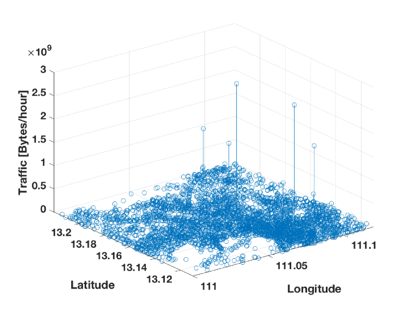
(a) Raw traffic data on the 22th Aug. 2012 6pm [34].

.

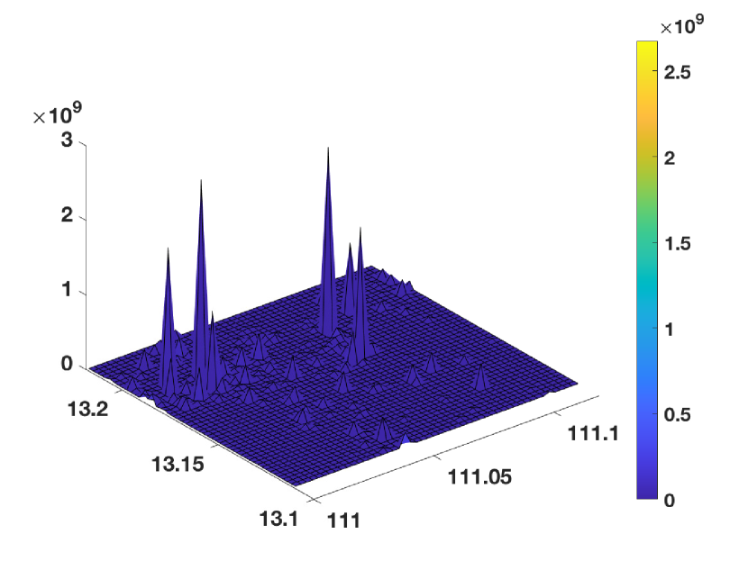
(b) First smoothing: data aggregation at drone coverage level.

Figure 6: Data preprocessing: raw data and first smoothing.

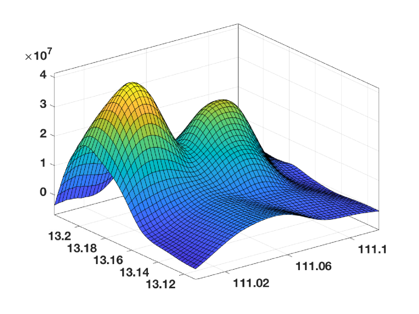
(a) Second smoothing: LOWESS with $\alpha=0.25$.

(b) K-means partition.

Figure 7: Data preprocessing: second smoothing and partitions in 2 phases.

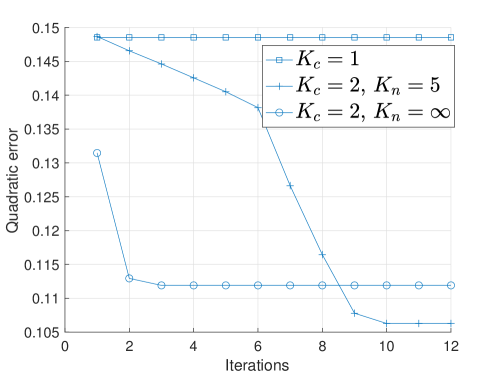
Figure 8: Quadratic error between normalized smoothed data and quadratic models.

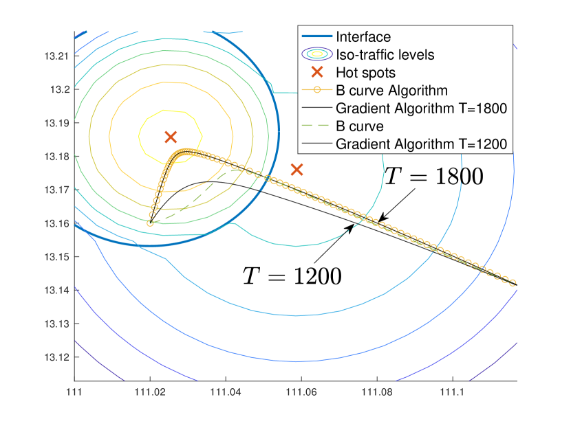
(a) $K=60$, $T=1200$ and $1800$, 2 phases.

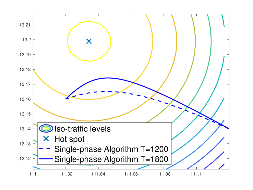
(b) $K=60$, $T=1200$ s and $1800$ s, 1 phase.

Figure 9: Influence of $T$ on the optimal trajectory.

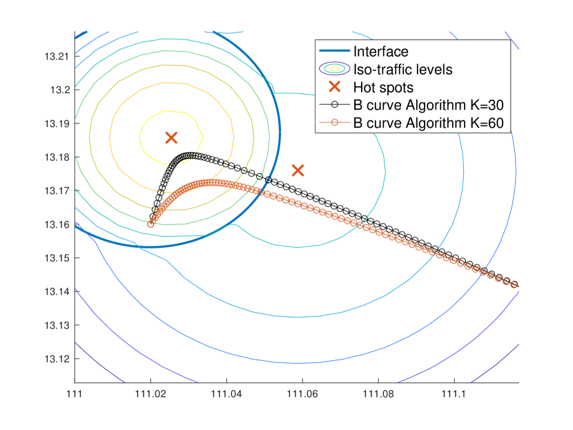
(a) $K=30$ and $60$, $T=1200$, 2 phases.

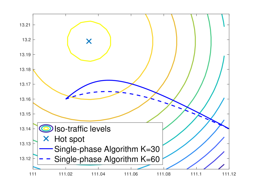
(b) $K=30$ and $60$, $T=1200$ s, 1 phase.

Figure 10: Influence of $K$ on the optimal trajectory.

V-B Trajectory optimization results

V-B1 Estimation procedure of parameters K and T

as in most similar algorithms, a ’prior’ estimation of parameters is necessary since the optimal results strongly depend on them. Traffic parameters have been estimated just above, so the required parameters are first the mass $K$ representing trade-off between the kinetic term and the traffic term in Lagrangian (2) and then the total duration time $T$ which has also a significant influence on the optimal trajectory (by convention $t_{0}=0$). This procedure is developed in Appendix -G and yields in our case:

$$T\approx 850,K=50\times r^{2}\mbox{ with }r=\frac{40\times 10^{6}}{360\times 100}\mbox{ and we select: }T=1200,1800s\mbox{ and }K=30,60\times r^{2}.$$

V-B2 Results

$$\begin{array}[]{|c c c c c | l | }\hline\cr\hline\cr\vspace*{1mm}\xi&{\mathbf{S}}&H^{-}&\phi^{-}&\phi^{+}&\tau\\ \hline\cr\hline\cr\vrule\lx@intercol\hfil\mathbf{a)}\ K=60\times r^{2}\enspace,\ T=1200\ \rightarrow S_{1ph}=-221.4103\hfil\lx@intercol\vrule\lx@intercol\\[2.84526pt] \vrule\lx@intercol\hfil\mbox{{B-Algo}}\ (Niter=12)\hfil\lx@intercol\vrule\lx@intercol\\ ({111.048},{13.170})&-168.5713&0.8131&1.9803&0.9236&538.69\\[2.84526pt] \hline\cr\vrule\lx@intercol\hfil\mbox{{Grad-Algo} }(Niter=5)\hfil\lx@intercol\vrule\lx@intercol\\ ({111.048},{13.170})&-168.5713&0.8131&1.9802&0.9237&538.68\\ \hline\cr\hline\cr\vrule\lx@intercol\hfil\mathbf{b)}\ K=60\times r^{2}\enspace,\ T=1800\ \rightarrow S_{1ph}=-637.9077\hfil\lx@intercol\vrule\lx@intercol\\[2.84526pt] \vrule\lx@intercol\hfil\mbox{{B-Algo}}\ (Niter=12)\hfil\lx@intercol\vrule\lx@intercol\\ ({111.0511},{13.1734})&-641.6388&0.8332&4.1764&0.9273&1136.09\\[2.84526pt] \hline\cr\vrule\lx@intercol\hfil\mbox{{Grad-Algo} }(Niter=2)\hfil\lx@intercol\vrule\lx@intercol\\ ({111.0511},{13.1734})&-641.6388&0.8332&4.1763&0.9273&1136.08\\ \hline\cr\hline\cr\vrule\lx@intercol\hfil\mathbf{c)}\ K=30\times r^{2}\enspace,\ T=1200\ \rightarrow S_{1ph}=-399.1474\hfil\lx@intercol\vrule\lx@intercol\\[2.84526pt] \vrule\lx@intercol\hfil\mbox{{B-Algo}}\ (Niter=12)\hfil\lx@intercol\vrule\lx@intercol\\ ({111.051},{13.173})&-393.1217&0.8313&3.7936&0.9289&729.71\\[2.84526pt] \hline\cr\vrule\lx@intercol\hfil\mbox{{Grad-Algo} }(Niter=2)\hfil\lx@intercol\vrule\lx@intercol\\ ({11.051},{13.173})&-393.1217&0.8313&3.7933&0.9290&729.65\\ \hline\cr\end{array}$$

TABLE I: Table of results with B-Algo and Grad-Algo for $K=30,60\times r^{2}$ , $T=1200,1800s$
and $r=\frac{40\times 10^{6}}{360\times 100}\approx 1111.1111$ (corresponding to scaled spatial unity of 100m).
Also, $S_{1ph}$ denotes the total single-phase cost (i.e., assuming only one, effective hotspot).

$$\begin{array}[]{| l | c c | c c |}\hline\cr\hline\cr\vrule\lx@intercol case\hfil\lx@intercol\vrule\lx@intercol&\lx@intercol\hfil\mbox{bi-phase}\hfil\lx@intercol\vrule\lx@intercol&\lx@intercol\hfil\mbox{single-phase}\hfil\lx@intercol\vrule\lx@intercol\\[2.84526pt] &L\ (\mbox{km})&\bar{V}(\mbox{m/s})&L\ (\mbox{km})&\bar{V}(\mbox{m/s})\\ \hline\cr{\mathbf{a)}}&12.41&10.34&11.71&9.76\\[2.84526pt] \hline\cr{\mathbf{b)}}&13.80&7.66&12.53&6.96\\[2.84526pt] \hline\cr{\mathbf{c)}}&13.64&11.37&12.37&10.30\\ \hline\cr\end{array}$$

TABLE II: Table of trajectory lengths and related average speeds.

optimal trajectories are shown in Figs. 9 and 10 and related numerical results in Table I.
Length of various trajectories and related average velocities are given in Table II.
The following main comments can be made on these results:

• First the obtained trajectories for Grad-Algo and B-Algo satisfy both the optimal conditions, as “relative” discrepancies between impulsions and between Hamiltonians at the interface are indeed below selected precision of $2.10^{-4}$, numerically yielding a full trajectory,

• Then Grad-Algo is found to be stable due to our choice of initial and terminal drone positions (not too close to the interface and not too far from their related hotspots) and of time intervals (not too large temporal phases). Thus, we are far from the non-convexity conditions expressed in Theorems 3 and 4. The positivity of the total hessian is indeed constantly checked at each iteration. Hence, a large (spatio-temporal) convergence basin resulting into exact convergence of the Grad-Algo (as well as the B-Algo) towards the unique optimal solution.

• As already noted for the single-phase case (paragraph III-A2), decreasing mass $K$ enables the drone to collect more traffic. In fact, during the allowed time interval, the drone will get closer to the hotspot with maximal traffic in order to decrease the total value function, i.e., zone $1$ here.

• Increasing time interval ($T\nearrow$) will produce the same tendancy, allowing the drone to spend more time near the hotspot with higher traffic $z_{h1}$, see Figs. 9(a) and 10(a).

• Since the drone has enough time to pick up traffic located close to hotspots, this is reflected in an average drone velocity about half its nominal value (see Table II).

VI Conclusion

In this paper, we propose a Lagrangian approach to solve the UAV base station optimal trajectory problem. When the traffic intensity exhibits a single phase, closed-form expressions for the trajectory and speed are derived from Hamilton-Jacobi equations. When the traffic intensity exhibits multiple phases, we characterize the crossing time and location at the interface. We propose two low-complexity algorithms for the bi-phase time-stationary traffic case that provide optimal crossing time and location on the interface and fulfill the necessary conditions of optimality. At last, we present a data processing procedure based on a modified K-means algorithm that derives a single-phase or bi-phase quadratic model from real traffic data. Further extensions of this work are envisioned to generalize the approach to three or more hot-spots and to consider multi-drone coordinated trajectories.

-A Proof of Lemma 1

In a neighborhood of the optimal trajectory, the first order variation of $S$ is null

$$\delta S = \int_{t_{0}}^{T}\delta\mathcal{L}(t,z,a)dt$$

$$= \int_{t_{0}}^{T}\left[\nabla_{z}\mathcal{L}(t,z,a)\cdot\delta z(t)+\nabla_{a}\mathcal{L}(t,z,a)\cdot\delta a(t)\right]dt.$$

We now note that $\delta a=\delta\frac{dz}{dt}=\frac{d(\delta z)}{dt}$. Integrating by part the second term in the integral of $\delta S$, we obtain

$$\int_{t_{0}}^{T}\nabla_{a}\mathcal{L}(t,z,a)\cdot\frac{d(\delta z)}{dt}dt$$

$$= [\delta z(t)\cdot\nabla_{a}\mathcal{L}(t,z,a)]_{t_{0}}^{T}-\int_{t_{0}}^{T}\delta z(t)\cdot\frac{d}{dt}\nabla_{a}\mathcal{L}(t,z,a)dt.$$

Note that $[\delta z\frac{\partial\mathcal{L}}{\partial a}]_{t_{0}}^{T}=0$ because $z_{0}$ and $z_{T}$ are fixed. Equating $\delta S$ to zero gives

$$0=\int_{t_{0}}^{T}\left[\nabla_{z}\mathcal{L}(t,z,a)-\frac{d}{dt}\nabla_{a}\mathcal{L}(t,z,a)\right]\cdot\delta z(t)dt.$$ (42)

As this should be true for every $\delta z$, $\mathcal{L}$, $z_{0}$ and $z_{T}$, we obtain the first result.

Now assume that we have the optimal $a(t)$, the condition for $z(T)$ to be the optimal final position is

$$\delta S = [\delta z(t)\cdot\nabla_{a}\mathcal{L}(t,z,a)]_{t_{0}}^{T}+\nabla J(z(T))\cdot\delta z(T)$$ (43)

$$= \nabla_{a}\mathcal{L}(z(T),T,a(T))\cdot\delta z(T)+\nabla J(z(T))\cdot\delta z(T)$$

$$= 0.$$

Note that $z_{0}$ is fixed and so $\delta z$ in $z_{0}$ is null. We thus obtain the second result of the lemma.

-B Proof of Lemma 2

As $\mathcal{L}(z,a)$ is an homogeneous function of $z$ and $a$, we have: $\mathcal{L}(\lambda z,\lambda a)=|\lambda|^{\alpha}\mathcal{L}(z,a)$ for all $\lambda$ (in our case with $\alpha=2$). Deriving this expression with respect to $\lambda$, setting $\lambda=1$, and noting that $a=\dot{z}$ we obtain

$$z\cdot\frac{\partial\mathcal{L}(z,\dot{z})}{\partial z}+\dot{z}\cdot\frac{\partial\mathcal{L}(z,\dot{z})}{\partial z} = \alpha\mathcal{L}(z,\dot{z}).$$ (44)

Using (7) and (44), we have: $z\cdot\frac{dp}{dt}+\dot{z}\cdot p=\alpha\mathcal{L}$ or equivalently $\frac{d(p\cdot z)}{dt}=\alpha\mathcal{L}$. We can now integrate the cost function (3) along the optimal trajectory as follows

$$S(t_{0},z_{0},T,z_{T}) = \frac{1}{\alpha}\int_{t_{0}}^{T}\frac{d(p\cdot z)}{dt}(t)dt+J(z_{T})$$ (45)

$$= \frac{1}{\alpha}\left(p(T)\cdot z_{T}-p(t_{0})\cdot z_{0}\right)+J(z_{T})$$

-C Proof of Lemma 3

We assume that an optimal trajectory exists and we apply the principle of optimality on the optimal trajectory between $(t,z^{*}(t))$ and $(t+h,z^{*}(t)+ah)$, where $h>0$, to opbtain

$$S(t,z^{*}(t),T,z_{T}) = \min_{a}[h\mathcal{L}(z^{*}(t),a)+S(t+h,z^{*}(t)+ah,T,z_{T})]$$

$$= \min_{a}[h\mathcal{L}(z,a)+S(t,z^{*}(t),T,z_{T})+ha\cdot\nabla_{X_{1}}S(t,z^{*}(t),T,z_{T})+h\frac{\partial S}{\partial T_{1}}(t,z^{*}(t),T,z_{T})].$$

This implies that

$$\frac{\partial S}{\partial T_{1}}(t,z^{*}(t),T,z_{T}) = -\min_{a}[a\cdot\nabla_{X_{1}}S(t,z^{*}(t),T,z_{T})+\mathcal{L}(z^{*}(t),a)]$$

$$= \max_{a}[-a\cdot\nabla_{X_{1}}S(t,z^{*}(t),T,z_{T})-\mathcal{L}(z^{*}(t),a)]$$

$$= H(t,z^{*}(t),-\nabla_{X_{1}}S(t,z^{*}(t),T,z_{T})).$$

By using the same approach between $t-h$ and $t$, we deduce in the same way equation (10) when the final time $T$ is varying.

-D Proof of Theorem 1

From (6) and (12), we obtain the following ordinary differential equation of second degree: $\ddot{z}=-\frac{u_{0}}{K}z$. If $\frac{u_{0}}{K}>0$, we define $\omega^{2}=\frac{u_{0}}{K}$ and we look for an optimal trajectory of the form: $z(t)=A\cos(\omega t)+B\sin(\omega t)$. If $\frac{u_{0}}{K}<0$, we look for an optimal trajectory of the form: $z(t)=A\cosh(\omega t)+B\sinh(\omega t)$ with $\omega^{2}=-\frac{u_{0}}{K}$. Let us denote $z_{0}=z(t_{0})$ and $a_{0}=a(t_{0})$ the initial conditions for $z$ and $\dot{z}$.

Take the case $\frac{u_{0}}{K}<0$. Using the derivative of $z(t)$ and identifying terms, we obtain: $z(t)=z_{0}\cosh\omega(t-t_{0})+\frac{a_{0}}{\omega}\sinh\omega(t-t_{0})$. At $t=T$, we have also: $z_{T}=z_{0}\cosh\omega(T-t_{0})+\frac{a_{0}}{\omega}\sinh\omega(T-t_{0})$, from which we deduce

$$a(t_{0}) = \frac{\omega(z_{T}-z_{0}\cosh\omega(T-t_{0}))}{\sinh\omega(T-t_{0}))},$$ (46)

$$a(T) = \frac{\omega(-z_{0}+z_{T}\cosh\omega(T-t_{0}))}{\sinh\omega(T-t_{0}))}.$$ (47)

when $u_{0}<0$. In a similar way, we have

$$a(t_{0}) = \frac{\omega(z_{T}-z_{0}\cos\omega(T-t_{0}))}{\sin\omega(T-t_{0})},$$ (48)

$$a(T) = \frac{\omega(-z_{0}+z_{T}\cos\omega(T-t_{0}))}{\sin\omega(T-t_{0})},$$ (49)

when $u_{0}>0$. Injecting $a(t_{0})=a_{0}$ in the equation of the trajectory provides the result.

For the computation of $S$, we now use the result of Lemma 2 as our cost function is 2-homogeneous. From equation (8), we see that only initial and final conditions are required to compute the cost function. Recall now that $p=Ka$. Injecting the equations of $a(t_{0})$ and $a(T)$ in (8), we obtain the result for the cost function.

-E Proof of Theorem 2

We assume that the location and time $(\xi,\tau)$ of interface crossing is known and unique. The optimal trajectory between $(z_{0},t_{0})$ and $(z_{T},T)$ can be decomposed in two sub-trajectories that are themselves optimal between $(z_{0},t_{0})$ and $(\xi,\tau)$ on the one hand and between $(\xi,\tau)$ and $(z_{T},T)$ on the other hand, by the principle of optimality. In region 1, the optimal cost up to $\tau$ is

$$S_{1}(t_{0},z_{0},\tau,\xi)=\int_{t_{0}}^{\tau}\mathcal{L}(z^{*}(s),a^{*}(s))ds.$$ (50)

Using Hamilton-Jacobi, we obtain

$$\frac{\partial S_{1}}{\partial T_{2}}(t_{0},z_{0},\tau,\xi)=-H_{1}(\xi,p^{*}(\tau^{-})).$$ (51)

In the same way, the optimal cost in region 2 is

$$S_{2}(\tau,\xi,T,z_{T}) = \int_{\tau}^{T}\mathcal{L}(z^{*}(s),a^{*}(s))ds.$$ (52)

Using again Hamilton-Jacobi, we obtain

$$\frac{\partial S_{2}}{\partial T_{1}}(\tau,\xi,T,z_{T})=H_{2}(\xi,p^{*}(\tau^{+})).$$ (53)

A necessary condition for the optimality of $\tau$ is thus

$$\frac{\partial S_{1}}{\partial T_{2}}(t_{0},z_{0},\tau,\xi)+\frac{\partial S_{2}}{\partial T_{1}}(\tau,\xi,T,z_{T})=0,$$ (54)

that is

$$H_{1}(\xi,p^{*}(\tau^{-}))=H_{2}(\xi,p^{*}(\tau^{+})).$$ (55)

A necessary condition for the optimality of $\xi$ in the total cost under the constraint $f(\xi)=C$ is also

$$\mu\ \nabla_{z}f(\xi) = \nabla_{X_{2}}S_{1}(t_{0},z_{0},\tau,\xi)+\nabla_{X_{1}}S_{2}(\tau,\xi,T,z_{T})$$

$$= p^{*}(\tau^{-})-p^{*}(\tau^{+})$$

where $\mu$ is a Lagrange multiplier associated to the constraint and where the second line comes from equation (11) of Hamilton-Jacobi. Thus we obtain precisely equation (21).

-F The structure and the diagonalization of single- and two- phase Hessian of the value fonction

-F1 Proof of Theorem 3

Recall that we study the second-order differentiability properties of single-phase value function $S(t_{1},{x}_{1},t_{2},{x}_{2})$. Recall that from Eq. (1) we study Hessians of the form

$$\mathcal{M}_{1+2,1+2}(\mathbb{R})\ni\nabla^{2}\sigma=\begin{pmatrix}\dfrac{\partial^{2}{}}{\partial{T_{i}}^{2}}\ \sigma&\dfrac{\partial{}}{\partial{T_{i}}}\nabla_{Xi}\ \sigma\\ \nabla_{Xi}\dfrac{\partial{}}{\partial{T_{i}}}\ \sigma&\nabla^{2}_{X_{i},X_{i}}\ \sigma\end{pmatrix}\ \ \mbox{where }\sigma\mbox{ stands for }S(t_{1},{x}_{1},t_{2},{x}_{2})\mbox{ and }i=1,2$$

It is clear by inspecting the symmetries of (14) with respect to the spatial coordinates that

$$\nabla^{2}_{X_{1},X_{1}}S(t_{1},{x}_{1},t_{2},{x}_{2})=\nabla^{2}_{X_{2},X_{2}}S(t_{1},{x}_{1},t_{2},{x}_{2})=Kg\ \mbox{Id}_{2},$$

$$\mbox{where }g=\omega\ \coth\phi\ \ \ \mbox{and}\ \phi=\omega\ (t_{2}-t_{1})\mbox{ is the {\em temporal} phase}.$$ (56)

Concerning symmetry with respect to time variables, one also finds easily that

$$\dfrac{\partial^{2}{S}}{\partial{T_{1}}^{2}}(t_{1},{x}_{1},t_{2},{x}_{2})=\dfrac{\partial^{2}{S}}{\partial{T_{2}}^{2}}(t_{1},{x}_{1},t_{2},{x}_{2}).$$

The Hessian with respect to the variable $\chi_{i}$ = $(T_{i},X_{i})_{i=1,2}\in\mathbb{R}\times\mathbb{R}^{2}$ has thus the following structure:

$${\cal H}(\chi_{i}) =\left(\begin{array}[]{l | c}\alpha&\hskip 5.69054pt{\Pi_{i}}^{\dagger}\\[2.84526pt] \hline\cr\Pi_{i}&\hskip 11.38109ptK\ g\ \mbox{Id}_{2}\end{array}\right)\hskip 42.67912pt\mbox{with}\hskip 42.67912pt\left\{\begin{array}[]{l}\alpha=\dfrac{\partial^{2}{S}}{\partial{T_{1}}^{2}}=\dfrac{\partial^{2}{S}}{\partial{T_{2}}^{2}}\\[11.38109pt] g=\omega\ \coth\phi\\[11.38109pt] \Pi_{i}=\dfrac{\partial}{\partial T_{i}}{\nabla_{X_{i}}S}\end{array}\right.$$ (62)

where the vector $\Pi_{i}$ and real scalar $\alpha$ remain to be determined.
Now recall that initial and final impulsions ${p}_{1}$ and ${p}_{2}$ as given by (46) write:

$${p}_{1} =K\ \omega\ \dfrac{-{x}_{1}\cosh\phi+{x}_{2}}{\sinh\phi},$$ (63)

$${p}_{2} =K\ \omega\ \dfrac{-{x}_{1}+{x}_{2}\cosh\phi}{\sinh\phi}.$$ (64)

In fact the expression of $\Pi_{i}$ and $\alpha$ appearing in Hessian (62) result both from the computation of $\dfrac{\partial{p_{i}}}{\partial{T_{i}}}$ for $i=1,\ 2.$ Using (56), the differentiation of (63) and (64) wrt.  $T_{1}$ resp. $T_{2}$ leads to the following simple result

$$\Pi_{1}=\dfrac{\partial}{\partial T_{1}}{\nabla_{X_{1}}S}=\dfrac{\partial{{p}_{1}}}{\partial{T_{1}}}=-\ \omega\ \dfrac{{p}_{2}}{\sinh\phi}\ \ \ \mbox{ resp. }\ \ \Pi_{2}=\dfrac{\partial}{\partial T_{2}}{\nabla_{X_{2}}S}=\dfrac{\partial{{p}_{2}}}{\partial{T_{2}}}=-\ \omega\ \dfrac{{p}_{1}}{\sinh\phi}.$$ (65)

Now, as far as the second partial derivative of value function $S$ with respect to time ($\alpha$) is concerned

$$\alpha=\dfrac{\partial^{2}{S}}{\partial{T_{1}}^{2}}=-\dfrac{\partial{H}}{\partial{T_{1}}}\ \ \ \mbox{ (Hamilton-Jacobi) }$$ (66)

Recalling that the Hamiltonian for any Newtonian model has the form

$$H(z,p,t)=\dfrac{{\parallel{p}\parallel}^{2}}{2\ K}+V(z)$$ (67)

and differentiating it with respect to the temporal phase $\phi$ at fixed extremities ${x}_{1}$ and ${x}_{2}$ leads to

$$\delta\,H =\dfrac{{p}_{1}\cdot\delta\,{p}_{1}}{K}=\dfrac{{p}_{2}\cdot\delta\,{p}_{2}}{K}=-\dfrac{{p}_{1}\cdot{p}_{2}}{K\ \sinh\phi}\ \delta\,\phi\enspace,\ \ \mbox{that is}$$

$$\alpha =\dfrac{\partial^{2}{S}}{\partial{T_{1}}^{2}}=\dfrac{\partial^{2}{S}}{\partial{T_{2}}^{2}}=-\ \omega\ \dfrac{\partial{H}}{\partial{\phi}}=\dfrac{\omega}{K}\ \dfrac{{p}_{1}\cdot{p}_{2}}{\sinh\phi}.\qed$$ (68)

Now from (24) the two-phase Hessian is simply the sum of the two single-phase Hessians.

-F2 Diagonalizing the Hessian of single- and two- phase value function

since the Hessians of single- and two-phase value function do have the same structure, we address a general Hessian of the form (62).
Its characteristic polynom is easily developed as

$$\det\ ({\cal H}-\nu\ \mbox{Id}_{3})=(Kg-\nu)^{2}\ (\alpha-\nu)-\,(Kg-\nu)\ \parallel{\Pi}\parallel{}^{2}.$$

Since from (62) one has $\forall({\theta},\,{x})\in\mathbb{R}\times\mathbb{R}^{2}\ \ \ {\cal H}({\theta},\,{x})=({\alpha\ \theta+\Pi\cdot x},\,{\Pi\ \theta+Kg\ x})$,
the three real eigenvalues $(\nu_{i})_{i=0:2}$ and related eigenvectors $Y_{i}=(\theta_{i},x_{i})$ thus satisfy
$i)\ \text{if }\nu_{0}=Kg>0\text{ then}\\ Y_{0}=({\theta=0},\,{x_{0}})\mbox{ with }x_{0}\perp\Pi\enspace:\mbox{"pure space" eigenvector }Y_{0}\in\{0\}\times\mathbb{R}^{2},\\ ii)\ \text{if }\nu_{1},\ \nu_{2}\mbox{ such that }(Kg-\nu)\ (\alpha-\nu)\ -\parallel{\Pi}\parallel{}^{2}=0\text{ then }\\ Y_{i}={({\theta_{i}},\,{x_{i}=\Pi})}_{i=1,2}\enspace:\mbox{two (mutually orthogonal) eigenvectors orthogonal to }Y_{0}\ (\mbox{since }\Pi\perp x_{0})\\ \mbox{ with }\nu_{1}\ \nu_{2}=\alpha\ Kg\ -\parallel{\Pi}\parallel{}^{2}\ \ =\det({\cal H})\ /\ (Kg)\ \ \mbox{ and }\ \ \nu_{1}+\nu_{2}=\alpha+Kg.$
Thus $\nu_{1},\nu_{2}$ cannot be simultaneously negative since this would imply
$\alpha<-Kg<0\Rightarrow\det({\cal H})=\nu_{0}\ \nu_{1}\ \nu_{2}\ <0$.
However the condition $\alpha\ Kg\ <\ \parallel{\Pi}\parallel{}^{2}$ (e.g. induced by the sufficient condition $\alpha<0$) implies that one of eigenvalues $\nu_{1}\ ,\ \nu_{2}<0$   namely the local non-convexity of the Hessian matrix ${\cal H}$.
This property holds thus for each single-phase value function as well as for the total two-phase case.

-G Estimation of parameters

It is based on the following remarks. First, the interface location ${\cal I}$ is independent of $K$ and $T$ (since only depends on traffic variables). Then, final time $T$ remains always estimated in seconds $(t_{0}=0)$. Also, according to [38], a typical drone cell flights at speed $\bar{V}=20$ m/s and has an autonomy of about $28$ min. Last, we test our procedure for spatially-scaled data, where the convenient spatial unity is 100 m, so that the scaling ratio is

$$r=\frac{40.10^{6}}{360}\times 100\approx 1111.1111$$ (69)

Also, the following numerical estimations are considered

• for estimating $T$: the total length of the trajectory $L$ is approximated by

  $$L\approx c\ \times\parallel z_{0}-z_{T}\parallel\mbox{ with }c=1.5\rightarrow T=\frac{\bar{V}}{L}$$

  (recall that $T$ is un-scaled and stands in seconds.)

• for estimating $K$: the phase in each sub-trajectory should satisfy
  $\phi_{i}=\omega_{i}\ T_{i}<\phi_{max}\enspace,\ i=1,2$ where $\phi_{max}=10$ (also an un-scaled constant) .
  Then, spatial scaling by the quantity $r$ implies

  $$u_{0}^{i}\leftarrow\dfrac{u_{0}^{i}}{r^{2}}\enspace,i=1,2\enspace,\mbox{ and thus: }K\leftarrow\dfrac{K}{r^{2}}\mbox{ since }\ \ K\ \omega_{i}^{2}=u_{0}^{i}\ \mbox{ at any scale.}$$

Passing back into the original frame therefore implies that $K\leftarrow K\ r^{2}$.

References

- [1] Y. Zeng, Q. Wu, and R. Zhang, “Accessing from the sky: A tutorial on uav communications for 5g and beyond,” Proceedings of the IEEE, vol. 107, no. 12, pp. 2327–2375, 2019.
- [2] B. Pearre and T. X. Brown, “Model-free trajectory optimization for wireless data ferries among multiple sources,” in IEEE Globecom Workshops, Dec 2010, pp. 1793–1798.
- [3] V. Sharma, M. Bennis, and R. Kumar, “Uav-assisted heterogeneous networks for capacity enhancement,” IEEE Communications Letters, vol. 20, no. 6, pp. 1207–1210, June 2016.
- [4] D. Yang, Q. Wu, Y. Zeng, and R. Zhang, “Energy tradeoff in ground-to-uav communication via trajectory design,” IEEE Transactions on Vehicular Technology, vol. 67, no. 7, pp. 6721–6726, 2018.
- [5] T. T. Mac, C. Copot, D. T. Tran, and R. De Keyser, “Heuristic approaches in robot path planning: A survey,” Robotics and Autonomous Systems, vol. 86, pp. 13–28, 2016.
- [6] T.-Y. Chi, Y. Ming, S.-Y. Kuo, C.-C. Liao et al., “Civil uav path planning algorithm for considering connection with cellular data network,” in IEEE Intl. Conf. on Computer and Information Technology (CIT), June 2012, pp. 327–331.
- [7] D. Liberzon, Calculus of variations and optimal control theory: a concise introduction. Princeton University Press, 2011.
- [8] D. Delahaye, S. Puechmorel, P. Tsiotras, and E. Féron, “Mathematical models for aircraft trajectory design: A survey,” in Air Traffic Management and Systems. Springer, 2014, pp. 205–247.
- [9] Y. Zeng, R. Zhang, and T. J. Lim, “Throughput maximization for uav-enabled mobile relaying systems,” IEEE Transactions on Communications, vol. 64, no. 12, pp. 4983–4996, Dec 2016.
- [10] Y. Zeng and R. Zhang, “Energy-efficient uav communication with trajectory optimization,” IEEE Transactions on Wireless Communications, vol. 16, no. 6, pp. 3747–3760, June 2017.
- [11] Q. Wu, Y. Zeng, and R. Zhang, “Joint trajectory and communication design for multi-uav enabled wireless networks,” IEEE Transactions on Wireless Communications, vol. 17, no. 3, pp. 2109–2121, Mar. 2018.
- [12] Y. Zeng, J. Xu, and R. Zhang, “Energy minimization for wireless communication with rotary-wing uav,” IEEE Transactions on Wireless Communications, vol. 18, no. 4, pp. 2329–2345, 2019.
- [13] B. R. Marks and G. P. Wright, “A general inner approximation algorithm for nonconvex mathematical programs,” Operations research, vol. 26, no. 4, pp. 681–683, 1978.
- [14] J. Zhang, Y. Zeng, and R. Zhang, “Uav-enabled radio access network: Multi-mode communication and trajectory design,” IEEE Transactions on Signal Processing, vol. 66, no. 20, pp. 5269–5284, 2018.
- [15] O. von Stryk and R. Bulirsch, “Direct and indirect methods for trajectory optimization,” Annals of Operations Research, vol. 37, no. 1, pp. 357–373, Dec 1992.
- [16] G. Barles, A. Briani, and E. Trélat, “Value function and optimal trajectories for regional control problems via dynamic programming and Pontryagin maximum principles,” Math. Cont. Related Fields, to appear. [Online]. Available: https://www.ljll.math.upmc.fr/trelat/fichiers/BarBriTre.pdf
- [17] L. C. Evans, Partial differential equations, 2nd ed., ser. Graduate Studies in Mathematics. American Mathematical Society, Providence, RI, 2010, vol. 19.
- [18] M. Akian, S. Gaubert, and A. Lakhoua, “The max-plus finite element method for solving deterministic optimal control problems: basic properties and convergence analysis,” SIAM Journal on Control and Optimization, vol. 47, no. 2, pp. 817–848, 2008.
- [19] W. McEneaney, Max-plus methods for nonlinear control and estimation. Springer Science & Business Media, 2006.
- [20] A. Alla, M. Falcone, and L. Saluzzi, “An efficient DP algorithm on a tree-structure for finite horizon optimal control problems,” SIAM Journal on Scientific Computing, vol. 41, no. 4, pp. A2384–A2406, 2019.
- [21] S. Dolgov, D. Kalise, and K. Kunisch, “A tensor decomposition approach for high-dimensional Hamilton-Jacobi-Bellman equations,” arXiv preprint arXiv:1908.01533, 2019.
- [22] W. Kang and L. C. Wilcox, “Mitigating the curse of dimensionality: sparse grid characteristics method for optimal feedback control and HJB equations,” Computational Optimization and Applications, vol. 68, no. 2, pp. 289–315, 2017.
- [23] A. Alla, M. Falcone, and S. Volkwein, “Error analysis for POD approximations of infinite horizon problems via the dynamic programming approach,” SIAM Journal on Control and Optimization, vol. 55, no. 5, pp. 3091–3115, 2017.
- [24] D. Kalise, S. Kundu, and K. Kunisch, “Robust feedback control of nonlinear PDEs by numerical approximation of high-dimensional Hamilton-Jacobi-Isaacs equations,” arXiv preprint arXiv:1905.06276, 2019.
- [25] Y. T. Chow, J. Darbon, S. Osher, and W. Yin, “Algorithm for overcoming the curse of dimensionality for state-dependent Hamilton-Jacobi equations,” Journal of Computational Physics, vol. 387, pp. 376 – 409, 2019. [Online]. Available: http://www.sciencedirect.com/science/article/pii/S0021999119301093
- [26] J. Darbon and S. Osher, “Algorithms for overcoming the curse of dimensionality for certain Hamilton–Jacobi equations arising in control theory and elsewhere,” Research in the Mathematical Sciences, vol. 3, no. 1, p. 19, Sep 2016.
- [27] I. Yegorov and P. M. Dower, “Perspectives on characteristics based curse-of-dimensionality-free numerical approaches for solving Hamilton–Jacobi equations,” Applied Mathematics & Optimization, pp. 1–49, 2017.
- [28] Y. T. Chow, J. Darbon, S. Osher, and W. Yin, “Algorithm for overcoming the curse of dimensionality for certain non-convex Hamilton–Jacobi equations, projections and differential games,” Annals of Mathematical Sciences and Applications, vol. 3, no. 2, pp. 369–403, 2018.
- [29] T. Nakamura-Zimmerer, Q. Gong, and W. Kang, “Qrnet: Optimal regulator design with lqr-augmented neural networks,” IEEE Control Systems Letters, vol. 5, no. 4, pp. 1303–1308, 2021.
- [30] J. Han, A. Jentzen, and W. E, “Solving high-dimensional partial differential equations using deep learning,” Proceedings of the National Academy of Sciences, vol. 115, no. 34, pp. 8505–8510, 2018.
- [31] J. Darbon, G. P. Langlois, and T. Meng, “Overcoming the curse of dimensionality for some Hamilton–Jacobi partial differential equations via neural network architectures,” Research in the Mathematical Sciences, vol. 7, no. 3, Jul. 2020. [Online]. Available: https://doi.org/10.1007/s40687-020-00215-6
- [32] J. Darbon and T. Meng, “On some neural network architectures that can represent viscosity solutions of certain high dimensional Hamilton–Jacobi partial differential equations,” Journal of Computational Physics, vol. 425, p. 109907, 2021. [Online]. Available: http://www.sciencedirect.com/science/article/pii/S0021999120306811
- [33] M. Coupechoux, J. Darbon, J.-M. Kélif, and M. Sigelle, “Optimal trajectories of a uav base station using lagrangian mechanics,” in IEEE INFOCOM 2019-IEEE Conference on Computer Communications Workshops (INFOCOM WKSHPS). IEEE, 2019, pp. 626–631.
- [34] X. Chen, Y. Jin, S. Qiang, W. Hu, and K. Jiang, “Analyzing and modeling spatio-temporal dependence of cellular traffic at city scale,” in Communications (ICC), 2015 IEEE International Conference on, 2015.
- [35] M. Bierlaire, Optimization: Principles and Algorithm. EPFL Press, 2015.
- [36] W. S. Cleveland, “Robust locally weighted regression and smoothing scatterplots,” Journal of the American statistical association, vol. 74, no. 368, pp. 829–836, 1979.
- [37] K. Ueda and N. Yamashita, “On a global complexity bound of the levenberg-marquardt method,” Journal of optimization theory and applications, vol. 147, no. 3, pp. 443–453, 2010.
- [38] A. Fotouhi, M. Ding, and M. Hassan, “Dronecells: Improving 5g spectral efficiency using drone-mounted flying base stations,” arXiv preprint arXiv:1707.02041, 2017.