Noise and error analysis and optimization in particle-based kinetic plasma simulations

Abstract

In this paper we analyze the noise in macro-particle methods used in plasma physics and fluid dynamics, leading to approaches for minimizing the total error, focusing on electrostatic models in one dimension. We begin by describing kernel density estimation for continuous values of the spatial variable $x$, expressing the kernel in a form in which its shape and width are represented separately. The covariance matrix $C(x,y)$ of the noise in the density is computed, first for uniform true density. The band width of the covariance matrix is related to the width of the kernel. A feature that stands out is the presence of constant negative terms in the elements of the covariance matrix both on and off-diagonal. These negative correlations are related to the fact that the total number of particles is fixed at each time step; they also lead to the property $\int\!\,C(x,y)\,dy=0$. We investigate the effect of these negative correlations on the electric field computed by Gauss’s law, finding that the noise in the electric field is related to a process called the Ornstein-Uhlenbeck bridge, leading to a covariance matrix of the electric field with variance significantly reduced relative to that of a Brownian process.

For non-constant density, $\rho(x)$, still with continuous $x$, we analyze the total error in the density estimation and discuss it in terms of bias-variance optimization (BVO). For some characteristic length $l$, determined by the density and its second derivative, and kernel width $h$, having too few particles within $h$ leads to too much variance; for $h$ that is large relative to $l$, there is too much smoothing of the density. The optimum between these two limits is found by BVO. For kernels of the same width, it is shown that this optimum (minimum) is weakly sensitive to the kernel shape.

We repeat the analysis for $x$ discretized on a grid. In this case the charge deposition rule is determined by a particle shape. An important property to be respected in the discrete system is the exact preservation of total charge on the grid; this property is necessary to ensure that the electric field is equal at both ends, consistent with periodic boundary conditions. We find that if the particle shapes satisfy a sum rule, the particle charge deposited on the grid is conserved exactly. Further, if the particle shape is expressed as the convolution of a kernel with another kernel that satisfies the sum rule, then the particle shape obeys the sum rule. This property holds for kernels of arbitrary width, including widths that are not integer multiples of the grid spacing.

We show results relaxing the approximations used to do BVO optimization analytically, by doing numerical computations of the total error as a function of the kernel width, on a grid in $x$. The comparison between numerical and analytical results shows good agreement over a range of particle shapes.

We discuss the practical implications of our results, including the criteria for design and implementation of computationally efficient particles that take advantage of the developed theory.

1 Introduction

The particle-in-cell (PIC) method has been an indispensable tool of numerical modelers in fluid dynamics and kinetic plasma physics for several decades now [1, 2, 3, 4, 5, 6, 7, 8] and the variety of kinetic plasma problems to which it has been applied keeps increasing. The success of this method has spurred more recent developments [9, 10, 11, 12, 13, 14], with emphasis on geometrical aspects; for example, advantage has been taken of the Hamiltonian nature of the Vlasov-Maxwell system [15, 16]. To ensure conservation properties such as momentum, energy, charge, etc., some formulations [4, 11, 12, 17] rely on a variational method, related to the Hamiltonian prescription, while others devise specific spatial and temporal discretizations for providing conservation properties [9, 10, 17].

The first particle methods applied to plasma simulations [2] showed significant effects of noise due to a few factors: first, the deposition of a particle’s charge applied to only one grid node, an approach called the nearest grid point (NGP) method; second, very few particles were used, due to the limited computational power in the early 1970s; third, guidelines for noise minimization were quite limited.

The introduction of finite size computational particles by Birdsall and Langdon [3] significantly elevated the usefulness of the particle method. Indeed, a hierarchy of shapes, varying in size and smoothness, were proposed to address issues of noise [18, 19] as well as frequency aliasing [8].

The recognition that the level of particle noise scales as $N_{p}^{-1/2}$, where $N_{p}$ is the number of computational particles, together with ever-increasing demands for accuracy and fidelity of simulations has again put the issue of noise in particle methods in the spotlight. Advancement has come with the emergence of hybrid kinetic-fluid methods and the $\delta\!f$ method [20, 21, 22, 23, 24]. In spite of this progress, noise is still a limiting factor in particle codes: in $\delta\!f$ and hybrid methods particles are used to describe only a subset of the distribution function, however, noise is still an important factor for the particle part of the computations as well as for the fluid-particle coupling (for time-evolving fluids). In full kinetic treatments as well in hybrid and $\delta\!f$ methods, noise in the density is an especially serious problem for quasineutral plasmas, in which the local net charge density is small.

The present work presents a new analysis of the statistics of noise in particle-based methods. Specifically, we analyze the error in the estimation of the particle density in terms of a finite number of computational particles of finite size, a special case of kernel density estimation, with a focus on the bias-variance trade-off [25, 26]. We also analyze the error in the electric field computed from the charge density, showing that certain negative correlations in the density noise lead to properties of the electric field related to the Ornstein-Uhlenbeck bridge [27, 28, 29], a generalization of the Brownian bridge [30], a Brownian process with boundary conditions at each end. We concentrate on a 1D (one-dimensional) electrostatic (ES) formulation with periodic boundary conditions, with overall charge neutrality and immobile ions, leaving generalizations such as to higher dimensions and electromagnetic models for future work.

In Sec. 2 we establish the framework used in estimating the electron density and its noise properties in a $1$D electrostatic Vlasov-Poisson system. In this system, the only source of noise is the estimated charge density. (Electromagnetic models also involve noise in the estimated current density.) These issues related to density estimation are introduced with a continuous, i.e. non-discretized, spatial variable $x$. We also discuss the various kernels that can be used, show how the kernel width and its shape (smoothness) enter, and summarize some properties of these kernels that relate to discretization and that will enter in later sections.

In Sec. 3, and in the next section, we continue to restrict our attention to continuous $x$. We introduce the covariance matrix for the noise in the density, focusing in this section on a system in which the “true” density is uniform. We discuss the origin of certain negative terms in the covariance matrix. (These negative off-diagonal terms represent negative correlations.) We show that in computing the electric field by Gauss’s law, these negative correlations and the boundary conditions on the electric field lead to properties associated with the Ornstein-Uhlenbeck bridge. We characterize noise in the computed electric field in terms of its covariance matrix. We illustrate with a kernel involving a delta function. Issues associated with the Brownian bridge are discussed in more depth in Appendix A and issues related to relaxing the delta function restriction to give a nonzero kernel width are discussed in Appendix B.

In Section 4 we generalize to non-uniform density and discuss the application of bias-variance optimization [25] to find the optimal kernel width. This optimization in the presence of non-uniform density minimizes the total error in the density estimated with a kernel of a specific shape and width. This error consists of a variance term (noise) caused by the finite number of particles and a bias term, a smoothing of the density that occurs because of the finite kernel width. For the remainder of this paper we refer to noise as the error due to having a finite number of particles and the more general term error as including the bias. Issues relating to the scaling of the kernel width are discussed in Appendix C.

In Section 5 we discuss the density and electric field on a discrete grid, where a particle shape for the charge deposition enters. We discuss the importance of a sum rule; obeying this sum rule is a sufficient condition for the net charge on the grid to be exactly zero when the ion charge is subtracted. This requirement assures that the electric field at the endpoints are equal. We also show that for a general kernel, the sum rule is obeyed if the particle shape is a convolution of the kernel with another kernel that already satisfies the sum rule. We discuss the covariance matrix of the noise on the discrete grid for various particle shapes.

In Sec. 6 we compute the total error (bias plus variance) numerically for various shapes and compare with the analytic theory of sections 3 and 4.

In Sec. 7 we summarize and discuss our results.

2 Kernel density estimation by a finite number of particles

Particle methods are hybrid Lagrangian-Eulerian in nature: computational macro-particles are allowed to move with continuous positions and velocities, while charge densities and fields are resolved on a fixed computational grid. The connection between particles and grid is via a particle shape, which specifies a charge deposition rule. It has been traditional [8] to use particle sizes that are integer number of computational cells wide, although such restriction is not necessary; a related issue, which we also discuss in Sec. 5.1, is that the width of a particle shape and its degree of smoothness need not be related. The latter point has been emphasized in Ref. [12]. Furthermore, grid size is many times determined subjectively by the modeler according to a desired resolution, accuracy, the particular physics problem under consideration, etc. This resolution may be increased a few times to determine convergence of the numerical results, while also increasing the number of particles; a typical quantity that is kept constant is the average number of particles per cell. Of course, every time the grid resolution and particle number are increased, the demand for computational resources increases and for large problems this strategy quickly becomes prohibitive. The analysis in this paper aims to provide a systematic way of minimizing noise and error in the charge density by selecting optimal size and number of particles and, as a consequence, to minimize the computational resources required to achieve a given accuracy.

Our discussion will focus on 1D electrostatic models, in periodic geometry. As will be shown in the following, the charge density and its gradients are essential for the analysis of noise and error. Therefore, we consider working with quantities that are periodic functions of $x$ on the real interval $[0,1]$, but over all real values of the particle velocity $v$. This choice is advantageous for the presentation of the ideas, postponing grid discretization to later sections.

We introduce a representation of the electron distribution function in phase space $(x,v)\in[0,1]\times(-\infty,\infty)$ in terms of $N_{p}$ number of finite-size computational particles,

$$f_{e}(x,v,t)=\sum_{\mu=1}^{N_{p}}q_{\mu}K(x-\xi_{\mu})\delta(v-\dot{\xi}_{\mu})\,,$$ (1)

where $f_{e}$ is the estimated phase space distribution, $q_{\mu}$ is the computational particle charge, $\xi_{\mu}$ is the computational particle position, and $\dot{\xi}_{\mu}$ is its velocity. We use $q_{\mu}>0$ in Eq. (1) and throughout the presentation and the negative sign of the electron charge is added explicitly in places where it is used, e.g., in Gauss’s law (so strictly speaking $q_{\mu}$ is the weight and the macro-particle charge is $-q_{\mu}$). The general form of the kernel is $K(x,\xi)$, however, due to the periodic boundary conditions it assumes the translationally invariant form $K(x-\xi)$ (see below). The subscript “e” in Eq. (1) and everywhere throughout the paper stands for “estimated.” Also, for the rest of the paper we use the term particle in place of computational particle or macro-particle. This particle is usually comprised of many physical particles.

By integrating over velocity space, we obtain the estimated density of the electrons at any spatial point $x$ in terms of the positions of all of the particles:

$$\rho_{e}(x)=\sum_{\mu=1}^{N_{p}}q_{\mu}K(x-\xi_{\mu})\,.$$ (2)

We take the special case, in which all the $q_{\mu}$ are equal. With periodic boundary conditions on $[0,1]$, no particles are gained or lost, so $\int_{0}^{1}\rho_{e}(x)\,dx$ is conserved. We normalize to $\int_{0}^{1}\rho_{e}(x)dx=1$ and assume immobile ions with uniform, fixed density $\rho^{(i)}(x)$. Overall neutrality is assumed, i.e. $\int_{0}^{1}\rho^{(i)}(x)dx=1$ as well.

The form in Eq. (2) is the usual form of kernel density estimation, used in statistics and machine learning[25]. The kernel $K(x)$ is usually assumed to satisfy the following conditions, which do not present practical limitations:

•   Normalized to unity,

$$\mbox{\hskip 20.0pt}\int_{0}^{1}\!\,K(x)\,dx=1\,;$$ (3)

$$\mbox{\textbullet\,\, Symmetric, }K(x)=K(-x),\quad x\in[0,1];$$ (4)

$$\mbox{\textbullet\,\, Translationally invariant, }K(x,\xi)=K(x-\xi),\quad x,\xi\in[0,1];$$ (5)

$$\mbox{\textbullet\,\, Nonnegative, }K(x)\geq 0,\quad x\in[0,1];$$ (6)

•   Has compact support. (7)

Condition (3) ensures the density normalization discussed above while conditions (4)–(7) are chosen out of convenience but are not essential for the theory development. The normalization condition on the kernel and the condition $\int\rho_{e}(x)dx=1$ imply $\sum_{\mu=1}^{N_{p}}q_{\mu}=1$ while the assumed equal and constant particle charges lead to $q_{\mu}=1/N_{p}$.

At this stage, there is no grid, so the kernel width is not related to a grid spacing. We, in fact, express a kernel of width $h$ as

$$K(x)=\frac{1}{h}K_{f}\left(\frac{x}{h}\right),$$ (8)

where $K_{f}$ is the fundamental kernel with support $[-1/2,1/2]$. Thus, $K_{f}$ contains all the information on the particle shape, including its smoothness, while its width is independently set by $h$. (To be specific, we assume that $K_{f}$ is defined on the real line, and after scaling to form $K(x)$, it is extended to be periodic with period unity.)

Examples of fundamental kernels are given in Table 1 and illustrated in Fig. 1. The boxcar, linear and quadratic kernels are the convolutional particle shapes of Ref. [7, 8], scaled to the unit interval; the trapezoidal kernel is discussed in the following sections. Another important kernel is the Epanechnikov kernel [31]. Sec. 4.1 discusses the BVO process, optimal kernel width, etc., where the shape factors $\int\!K_{f}(x)^{2}\,dx$ and $\int\!x^{2}K_{f}(x)\,dx$, which are of order unity, play a prominent role.

In sections 5 and 6 we will apply these results involving the kernel $K(x)$ in the presence of a uniform grid $x_{i}$, $i=1,2,\ldots,N_{g}$ with spacing $\Delta=1/N_{g}$. There we will construct a particle shape $S(x)$, which satisfies conditions (3)-(7) for a kernel and also satisfies a sum rule

$$\sum_{i=1}^{N_{g}}\Delta\,S(x_{i}-\xi)=1\,$$ (9)

for an arbitrary particle position $\xi$, the discrete analog of the normalization condition in Eq. (3). We will show that a sufficient condition for $S(x)$ to satisfy the sum rule is that it be a convolution of a kernel of arbitrary width $\delta$ with either another particle shape or a finite element of width $i\Delta,\,i=1,2,\dots$; thereby, $S(x)$ can have an arbitrary width $h=i\Delta+\delta$.

As a last comment in this section, we note that not every kernel when scaled to a grid satisfies the sum rule; among our examples, the Epanechnikov kernel scaled to the grid spacing (width $h=i\Delta+\delta$) does not obey the sum rule (9) for any $\delta$ and $i=1,2,\dots$. In contrast, the boxcar, linear, quadratic, and trapezoidal kernels, when scaled to $h=\Delta,\,2\Delta,\,3\Delta$, $3\Delta$, correspondingly [cf. Eq. (8)], do satisfy the sum rule. We shall discuss these issues further in Sections 5 and 6. At the same time, since all particle shapes satisfy conditions (3)–(7), any particle shape may be used as a kernel in the density estimation expression (2).

Kernel	Definition
Boxcar (top-hat)	$K_{fB}(x)=\left\{\begin{tabular}[]{ll}$1$, $|x|\leq\frac{1}{2}$\\[4.30554pt] $0$ otherwise\,.\end{tabular}\right.$
Linear (tent)	$K_{fL}(x)=\left\{\begin{tabular}[]{ll}$2\left(1-2|x|\right)$, $|x|\leq\frac{1}{2}$\\[4.30554pt] $0$ otherwise\,.\end{tabular}\right.$
Quadratic	$K_{fQ}(x)=9\left\{\begin{tabular}[]{ll}$\frac{1}{4}-3x^{2}$, $\left|x\right|\leq 1/6$\\[4.30554pt] $\frac{3}{2}\left(\frac{1}{2}-|x|\right)^{2}$, $1/6\leq\left|x\right|\leq 1/2$\\[4.30554pt] $0$ otherwise\,.\end{tabular}\right.$
Trapezoidal	$K_{fT}(x)=\frac{3}{2}\left\{\begin{tabular}[]{ll}1, $|x|\leq 1/6$\\[4.30554pt] $3\left(\frac{1}{2}-|x|\right)$, $1/6\leq|x|\leq 1/2$\\[4.30554pt] $0$ otherwise\,.\end{tabular}\right.$
Epanechnikov	$K_{fE}(x)=\left\{\begin{tabular}[]{ll}$\frac{3}{2}\left(1-4x^{2}\right)$, $|x|\leq\frac{1}{2}$\\[4.30554pt] $0$ otherwise\,,\end{tabular}\right.$

Table 1: Examples of fundamental kernels, with width unity and normalized to have $\int K(x)dx=1$.

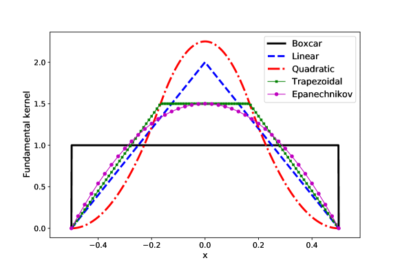
Figure 1: Illustration of the fundamental kernel examples from Table 1, normalized to unity. The important issues of bias-variance optimization and the sum rule in Eq. (9) are discussed in the text.

3 Statistical analysis in uniform density

Based on the kernel representation from Sec. 2, we analyze in this section what is typically known as “noise” in the PIC method. We note that—as will become clear in the next section—noise is only one part of the total error that we make when estimating the “true” density (or field) with the help of a finite number of particles, the other part being the bias error. When estimating the error in a uniform density, as we do in this section, only the noise part appears, the bias part being zero for this case. The focus is on the covariance matrix between the noise in the density at different spatial points. Based on the density covariance matrix, we consider the covariance matrix between the noise in the electric field at different spatial points.

3.1 Statistical analysis of the estimated density

In this section we introduce the mathematical method of the analyses of noise, and later that of error, while also deriving the uniform density correlations with the important negative contributions resulting from the fixed number of particles in a numerical simulation. Let us denote the true electron density by $\rho(x)$. Because of our choice of normalization, the true electron density (or true density) satisfies all the properties of a probability density function, and the normalization condition (3) guarantees that $\rho_{e}(x)$ does also. As discussed above, at this point in our analysis we do not consider grid discretization and hence we do not relate the kernel width $h$ to the grid spacing $\Delta$. Using the continuous spatial variable $x$, the average of any quantity $f(x)$ is calculated as

$$\left<f\right>=\int_{0}^{1}\!\!\,f(\xi)\rho(\xi)\,d\xi$$ (10)

or

$$\left<f\right>=\int_{0}^{1}\!\!f(\xi,\eta)\rho(\xi)\rho(\eta)\,d\xi d\eta$$ (11)

for a function of two random variables, etc. In this way, we can calculate the expected (statistical expectation) value of the estimated density over the true density $\rho(x)$ as

$$\langle\rho_{e}(x)\rangle= \left(\sum_{\mu}q_{\mu}\right)\int_{0}^{1}K(x-\xi)\rho(\xi)d\xi$$

$$= \int_{x-h/2}^{x+h/2}K_{f}\left(\frac{x-\xi}{h}\right)\rho(\xi)\frac{d\xi}{h}=\int_{-1/2}^{1/2}K_{f}(\eta)\rho(x+h\eta)d\eta,$$ (12)

where $\sum_{\mu}q_{\mu}=1$ has been used, the symmetry of $K$ has been used, and we have defined $\eta=(\xi-x)/h$. Expanding for small $h$, we find

$$\langle\rho_{e}(x)\rangle =\rho(x)\int_{-1/2}^{1/2}K_{f}(\eta)d\eta+\frac{h^{2}}{2}\rho^{\prime\prime}(x)\int_{-1/2}^{1/2}K_{f}(\eta)\eta^{2}d\eta+\cdots$$

$$=\rho(x)+\frac{h^{2}}{2}\rho^{\prime\prime}(x)\int_{-1/2}^{1/2}K_{f}(\eta)\eta^{2}d\eta+\cdots\,.$$ (13)

where the normalization $\int_{-1/2}^{1/2}K_{f}(\eta)d\eta=1$ condition has been used and the symmetry of $K_{f}$ has again been used to conclude $\int_{-1/2}^{1/2}K_{f}(\eta)\eta d\eta=0$. (Henceforth, we omit integral limits to improve readability.) We defer the issues of a non-uniform density $\rho(x)$ to a later section.

For the uniform density case considered in this section, $\rho(x)=1$ (hence $\rho^{\prime\prime}(x)=0$), and we obtain

$$\langle\rho_{e}(x)\rangle=\rho(x)=1.$$

Now defining the fluctuations $\tilde{\rho}_{e}(x)$ by $\rho_{e}(x)=\langle\rho_{e}(x)\rangle+\tilde{\rho}_{e}(x)=1+\tilde{\rho}_{e}(x)$ (note that $\left<\tilde{\rho}_{e}(x)\right>=0$), we can write the variance as $V(x)=\langle\tilde{\rho}_{e}(x)^{2}\rangle=\langle\rho_{e}(x)^{2}\rangle-1$, or

$$V(x)=V_{d}(x)+V_{o}(x)-1$$

where $V_{d}(x)$ and $V_{o}(x)$ denote the diagonal ($\mu=\nu$) and off-diagonal ($\mu\neq\nu$) terms in $V(x)$, as defined below. We find

$$V_{d}(x)=\sum_{\mu}q_{\mu}^{2}\langle K(x-\xi_{\mu})^{2}\rangle=\frac{1}{N_{p}}\int K(x-\xi)^{2}d\xi=\frac{1}{N_{p}}\int K(\xi)^{2}d\xi$$ (14)

and

$$V_{o}(x)= \,\sum_{\mu\neq\nu}q_{\mu}q_{\nu}\langle K(x-\xi_{\mu})K(x-\xi_{\nu})\rangle$$

$$= \,\frac{N_{p}(N_{p}-1)}{N_{p}^{2}}\int K(x-\xi)K(x-\eta)d\xi d\eta$$

$$= \,\frac{N_{p}(N_{p}-1)}{N_{p}^{2}}\left(\int K(\xi)d\xi\right)^{2},$$

$$= \,1-\frac{1}{N_{p}}.$$ (15)

At this point we notice the general scaling $V_{d}=(1/N_{p}h)\int K_{f}(\eta)^{2}d\eta\sim 1/N_{p}h$, which follows by using Eq. (8). The quantity $N_{p}h$ is the expected number of particles over the width of the kernel. These results lead to

$$V(x)=V_{d}(x)-1/N_{p}.$$ (16)

To relate the estimated density at arbitrary spatial points, $x$ and $y$, we must compute the covariance matrix

$$C(x,y)=\langle\tilde{\rho}_{e}(x)\tilde{\rho}_{e}(y)\rangle=\langle\rho_{e}(x)\rho_{e}(y)\rangle-1\,.$$ (17)

We again use a decomposition into diagonal and off-diagonal terms:

$$C(x,y)=C_{d}(x,y)+C_{o}(x,y)-1\,.$$ (18)

The two contributions are

$$C_{d}(x,y)=C_{d}(x-y)=\frac{1}{N_{p}}\int K(x-\xi)K(y-\xi)d\xi=\frac{1}{N_{p}}\hat{K}(x-y),$$ (19)

where $\hat{K}$ is the convolution of $K$ with itself (a legitimate kernel according to Eqs. (3) - (7)), and

$$C_{o}(x,y) =\frac{N_{p}(N_{p}-1)}{N_{p}^{2}}\int K(x-\xi)K(y-\eta)d\xi d\eta$$

$$=\frac{N_{p}(N_{p}-1)}{N_{p}^{2}}\left(\int K(\xi)d\xi\right)^{2}$$

$$=1-\frac{1}{N_{p}}\,.$$ (20)

Putting (18), (19), and (20) together, we find

$$C(x,y)=\frac{1}{N_{p}}\left[\hat{K}(x-y)-1\right].$$ (21)

In the special case $K(x)=\delta(x)$ we have $\hat{K}(x-y)=\delta(x-y)$ and from Eq. (21) we obtain

$$C(x-y)=\frac{1}{N_{p}}\left[\delta(x-y)-1\right].$$ (22)

Notice the translational invariance form $C(x-y)$ and the presence of constant negative contributions $-1/N_{p}$ in the expressions for the variance ($x=y$) and the off-diagonal (correlation) terms ($x\neq y$). In particular, we have

$$\int\!\!\,C(x,y)\,dy=\int\!\!\,C(x-y)\,dy=0\,.$$ (23)

Indeed, $\int C_{d}(x-y)dy=(1/N_{p})\int\!\hat{K}(x-y)\,dy=1/N_{p}$ since $\int\!\!\,\hat{K}(x-y)\,dx=1$. We emphasize that the property in Eq. (23) is general, i.e., for any kernel. An alternative proof is given as follows. Recalling that $\int\!\rho_{e}(y)\,dy=1$, it follows that $\int\!\tilde{\rho}_{e}(y)\,dy=\int\!(\rho_{e}(y)-1)\,dy=0$. Then from the definition of correlations (17) we obtain

$$\int\!\!C(x,y)\,dy=\left<\tilde{\rho}_{e}(x)\int\!\!\tilde{\rho}_{e}(y)\right>\,dy=0\,.$$

The result Eq. (23) implies that the function defined by $u(x)=1$ is in the null space of the covariance matrix, i.e., is the eigenfunction with zero eigenvalue.

The significance of the negative correlations is further discussed in the next section.

3.2 Statistical analysis of the electric field

In particle codes, noise in the density leads to noise in the electric field, which in turn affects particle orbits. In this section we quantify the effect of density noise on the electric field. The quantification of errors in particle orbits due to errors in the electric field, leading in turn to density errors, i.e., “closing the loop,” will be the subject of future work.

In the electrostatic model the electric field is computed from Gauss’s law (we use the dimensionless form),

$$\frac{dE}{dx}=\rho^{(i)}-\rho_{e}=\rho_{q},$$ (24)

where $\rho_{q}$ is the estimated density, $\rho_{e}$ is the estimated electron density, and again, $\rho^{(i)}=1$ is the fixed background ion density. Because of the assumption that the net charge is exactly zero, $\int_{0}^{1}\rho_{q}(x)dx=0$, we have $E(0)=E(1)$, consistent with the assumed periodic boundary conditions. We also specify that there is no applied potential across the system, so that

$$\int_{0}^{1}E(z)dz=0.$$ (25)

To incorporate condition (25) in the solution of (24), we start with the general expression

$$\hat{E}(x)=\int_{x_{0}}^{x}\!\!\rho_{q}(z)\,dz\,,$$ (26)

where $\hat{E}$ satisfies Eq. (24) and $x_{0}$ is an arbitrary initial point of integration. We calculate the integral of $\hat{E}(x)$ over the periodic domain $[0,1]$:

$$R_{0}= \int_{0}^{1}\!\!\hat{E}(x)\,dx=\int_{0}^{1}\!\!dx\,\int_{x_{0}}^{x}\!\!\rho_{q}(z)\,dz=\left.x\,\int_{x_{0}}^{x}\!\!\rho_{q}(z)\,dz\right|_{x=0}^{x=1}-\int_{0}^{1}\!\!x\rho_{q}(x)\,dx$$

$$= \int_{x_{0}}^{1}\!\!\rho_{q}(z)\,dz-\int_{0}^{1}\!\!z\rho_{q}(z)\,dz=\int_{0}^{1}\!\!\rho_{q}(z)\,dz-\int_{0}^{x_{0}}\!\!\rho_{q}(z)\,dz-\int_{0}^{1}\!\!z\,\rho_{q}(z)\,dz$$

$$= -\int_{0}^{x_{0}}\!\!\rho_{q}(z)\,dz-\int_{0}^{1}\!\!x\,\rho_{q}(x)\,dx,$$

where in the last line we have used $\int_{0}^{1}\!\!\rho_{q}(z)\,dz=0$. The quantity $R_{0}$ depends on $x_{0}$. The quantity $R_{0}$ needs to be subtracted from $\hat{E}(x)$ in order to obtain an expression $E(x)$ satisfying Eq. (25):

$$E(x)= \hat{E}(x)-R_{0}$$

$$= {\int_{x_{0}}^{x}\!\!\rho_{q}(z)\,dz}+{\int_{0}^{x_{0}}\!\!\rho_{q}(z)\,dz}+\int_{0}^{1}\!\!x\,\rho_{q}(x)\,dx$$

$$= \int_{0}^{x}\!\!\rho_{q}(z)\,dz+\int_{0}^{1}\!\!x\rho_{q}(x)\,dx\equiv\,\,E_{1}(x)+E_{0}\,.$$ (27)

Expression (27) indicates the unsurprising fact that in a periodic system the initial point of integration $x_{0}$ can be chosen arbitrarily regardless of the functional form of $E(x)$.

To compute correlations, we use (27), with $E(x)=\langle E(x)\rangle+\tilde{E}(x)$, to find

$$C^{E}(x,y)=\langle\tilde{E}(x)\tilde{E}(y)\rangle=\langle\tilde{E}_{0}\tilde{E}_{0}\rangle+\langle\tilde{E}_{0}\tilde{E}_{1}(y)\rangle+\langle\tilde{E}_{1}(x)\tilde{E}_{0}\rangle+\langle\tilde{E}_{1}(x)\tilde{E}_{1}(y)\rangle.$$ (28)

Using $\rho_{q}=1-\rho_{e}=-\tilde{\rho}_{e}$, we find

$$C_{00}^{E}=\langle\tilde{E}_{0}\tilde{E}_{0}\rangle=\int_{0}^{1}zdz\int_{0}^{1}w\langle\tilde{\rho}_{e}(z)\tilde{\rho}_{e}(w)\rangle\,dw;$$ (29)

we also find

$$C_{10}^{E}(x)=\langle\tilde{E}_{1}(x)\tilde{E}_{0}\rangle=\int_{0}^{1}wdw\int_{0}^{x}\langle\tilde{\rho}_{e}(w)\tilde{\rho}_{e}(z)\rangle dz,$$ (30)

and similarly for $C_{01}(y)$, and (e.g., for $x>y$),

$$C_{11}^{E}(x,y)=\int_{0}^{x}dz\int_{0}^{y}\langle\tilde{\rho}_{e}(z)\tilde{\rho}_{e}(w)\rangle\,dw.$$ (31)

Putting these together, we have

$$C^{E}(x,y)= \int_{0}^{1}zdz\int_{0}^{1}wC(z,w)\,dw+\int_{0}^{1}wdw\int_{0}^{x}C(w,z)dz$$

$$+\int_{0}^{1}zdz\int_{0}^{y}C(z,w)dw+\int_{0}^{x}dz\int_{0}^{y}C(z,w)\,dw.$$ (32)

For the special $\delta$-function case of Eq. (22), a substitution into (32) yields

$$C^{E}(x,y)=\frac{1}{N_{p}}\left[\text{min}(x,y)-xy+\frac{x(x-1)}{2}+\frac{y(y-1)}{2}+\frac{1}{12}\right],$$ (33)

which is extended outside $0<x,y<1$ to be periodic in both arguments. Equation (33) can be cast into the form

$$C^{E}(x,y)=\frac{1}{2N_{p}}\left[-|x-y|+(x-y)^{2}+\frac{1}{6}\right],$$ (34)

showing explicitly the translational invariance $C^{E}(x,y)=C^{E}(x-y)$ and thus independence of the initial point of integration, $x_{0}$, in addition to the symmetry $C^{E}(-x)=C^{E}(x)$. The first term in Eq. (33), $\propto\text{min}(x,y)$, is the Brownian motion result, obtained by assuming a Poisson probability distribution of particle numbers in each differential region. The sum of the first two terms represents the Brownian bridge [32], a random walk with negative correlations that force the electric field to be equal at both ends $E(0)=E(1)=0$; the physical origin of this condition is the net neutrality of the plasma $\int\rho_{q}(x)dx=0$. The complete result (33) using the zero potential assumption (25) can be identified as the Ornstein-Uhlenbeck bridge [27]. The three different cases are discussed in more detail in Appendix A.

The electric field correlations $C^{E}(x-y)$ in Eq. (34) are plotted in Fig. 2 for a fixed value of $y$, showing a maximum at a cusp at $x=y$, with $C^{E}$ being negative over about three parts and positive over about two parts of the range of $x-y$. Also shown in Fig. 2 is the covariance matrix for the Poisson case (random walk) and for the Brownian bridge, neither having translational invariance, both with cusps at $x=y$. Notice that for the Poisson case $C^{E}(1,y)\neq C^{E}(0,y)$. For the Brownian bridge case, we have $C^{E}(1,y)=C^{E}(0,y)=0$. It is easy to show from Eq. (33) that for periodic boundary conditions $C^{E}$ for the Ornstein-Uhlenbeck bridge is maximal at the cusp at $x=y$ (and at every periodic image), it has a smooth minimum exactly between the maxima, and has continuous derivatives at the endpoints $x=0,1$. Notice that the Brownian bridge correlations are positive, but less than those of the Poisson case for $x>y$, whereas correlations for the Ornstein-Uhlenbeck case are negative over an appreciable region of $(x,y)$ and are significantly smaller in magnitude. Finally, note the aperiodic behavior of $C^{E}$ for the random walk and the cusps at $x=0$ and $x=1$ for the Brownian bridge. We have also computed $C^{E}(x-y)$ for $\hat{K}$ equal to the linear tent function kernel, which is the convolution of two boxcar kernels of finite width $h$ (rather than $\hat{K}(x)=\delta(x)$). The result for $h=0.2$ is shown shown in Fig. 2 as the “smooth” Ornstein-Uhlenbeck bridge.

The implications of the lower values of the correlations to particle methods is as follows. Smaller variances ($x=y$) are desirable because they correspond to lower noise level. For $x\neq y$, the lower level of the magnitude of the correlations is expected because of the property $\int\!C^{E}(x,y)\,dx=0$. Also, in a physical system, i.e., in the limit of large $N_{p}$, such correlations vanish; therefore lower $C^{E}(x,y)$ is expected to improve the fidelity of the numerical results.

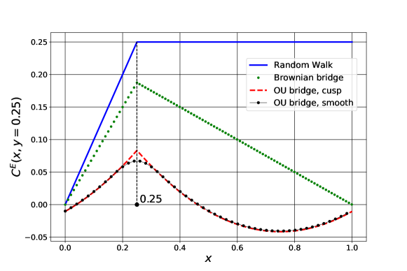
Figure 2: Comparison of the electric field covariance matrix $C^{E}(x,y)$, with $y=0.25$, for the random walk, the Brownian bridge, and the Ornstein-Uhlenbeck bridge. The black curve is the smooth Ornstein-Uhlenbeck bridge with a linear (tent) kernel of width $h=0.2$. Note that only the two Ornstein-Uhlenbeck bridge cases are periodic and have $C^{E}$ significantly reduced relative to the other two processes.

Recall that $\int\!C(x,y)\,dx=0$ [cf. Eq. (23)]. A similar general result can be derived for the electric field correlations $C^{E}$. Indeed, we have

$$\int_{0}^{1}C^{E}(x,y)dy=\left<\tilde{E}(x)\int_{0}^{1}\tilde{E}(y)dy\right>=0,$$ (35)

which vanishes because of the relation (25). In particular, (35) can be verified by a direct calculation for the special case of the covariance matrix (33) (or (34)). As noted for the density covariance matrix, the covariance $C^{E}$ also has an eigenfunction with eigenvalue zero, namely $\int_{0}^{1}C^{E}(x,y)u(y)dy=0$ for $u(y)=1$; we will return to this point in Sec. 5.

4 Statistical analysis of error in non-uniform density

In this section we discuss a statistical study of non-uniform density distributions. We now use the more general term “error” or “statistical error” instead of “noise,” as we will show that noise is only part of the total error, characterized by the variance, the other important contribution being the bias.

4.1 Optimal kernel size: bias-variance optimization

Let us evaluate the mean-square difference (error) $Q$ (henceforth simply error; the actual error can be calculated as $\sqrt{Q}$;) between the estimated density, $\rho_{e}(x)$, and the true density $\rho(x)$, where now $\rho(x)$ is not assumed to be constant. The quantity $Q$ is

$$Q=\left<\big{(}\rho_{e}(x)-\rho(x)\big{)}^{2}\right>=\left<\Big{(}\rho_{e}(x)-\left<{\rho}_{e}(x)\right>+\left<{\rho}_{e}(x)\right>-\rho(x)\Big{)}^{2}\right>\,,$$ (36)

where we remind the reader that $\langle f\rangle$ is given by Eq. (10) or (11). This quantity equals (omitting the argument $x$ for clarity)

$$Q=\left<\left(\rho_{e}-\left<{\rho}_{e}\right>\right)^{2}\right>+2\big{<}\left(\rho_{e}-\left<{\rho}_{e}\right>\right)\left(\left<{\rho}_{e}\right>-\rho\right)\big{>}+\left<\left(\left<{\rho}_{e}\right>-\rho\right)^{2}\right>\,.$$ (37)

We recognize that the factor $\left(\left<{\rho}_{e}(x)\right>-\rho(x)\right)$ in the middle and third terms is not a random variable; since the other factor in the middle term is zero, we find

$$Q=Q_{1}+Q_{2},$$ (38)

with

$$Q_{1}=\left<\rho_{e}^{2}\right>-\left<\rho_{e}\right>^{2},\qquad$$ (39)

$$Q_{2}=\big{(}\left<{\rho}_{e}\right>-\rho\big{)}^{2}.$$ (40)

To proceed, we go back to the Taylor expansion Eq. (13), noting that in a non-uniform density $\rho^{\prime\prime}(x)\neq 0$, and write it as

$$\langle\rho_{e}(x)\rangle=\rho(x)+B(x)+O(h^{4})$$ (41)

with

$$B(x)=h^{2}\frac{\rho^{\prime\prime}(x)}{2}\int\zeta^{2}K_{f}(\zeta)d\zeta\,.$$ (42)

The quantity $B(x)$ is called the statistical bias. Since $\int\!\left<\rho_{e}(x)\right>\,dx=1$, the bias satisfies $\int\!B(x)\,dx=0$, consistent with the periodic boundary conditions on $\rho(x)$.

For the first term in $Q_{1}$ we have

$$\langle\left(\rho_{e}(x)\right)^{2}\rangle=\sum_{\mu\nu}q_{\mu}q_{\nu}\langle K(x-\xi_{\mu})K(x-\xi_{\nu})\rangle$$

$$=\sum_{\mu}q_{\mu}^{2}\int K(x-\xi)^{2}\rho(\xi)d\xi+\sum_{\mu\neq\nu}q_{\mu}q_{\nu}\left(\int K(x-\xi)\rho(\xi)d\xi\right)^{2}\,,$$ (43)

where we have again split the sums into diagonal terms ($\mu=\nu$) and off-diagonal terms ($\mu\neq\nu$). Again, changing variables and Taylor expanding, we find

$$\langle\left(\rho_{e}(x)\right)^{2}\rangle= \,\,\frac{\rho(x)}{N_{p}h}\int K_{f}(\zeta)^{2}d\zeta+O\left(\frac{h}{N_{p}}\right)$$

$$+\left(1-\frac{1}{N_{p}}\right)\langle\rho_{e}(x)\rangle^{2}$$

$$\approx \,\,\frac{\rho(x)}{N_{p}h}\int K_{f}(\zeta)^{2}d\zeta+\langle\rho_{e}(x)\rangle^{2}-\frac{1}{N_{p}}\left(\rho(x)+B(x)\right)^{2}$$

$$= \,\,\frac{\rho(x)}{N_{p}h}\int K_{f}(\zeta)^{2}d\zeta+\langle\rho_{e}(x)\rangle^{2}-\frac{1}{N_{p}}\rho(x)^{2}\,,$$ (44)

using Eq. (41) and neglecting terms of first and higher orders in $h/N_{p}$. Note that the $-\rho(x)^{2}/N_{p}$ term in (44) does not arise from the Taylor expansion (13). For the purpose of the present argument we neglect that term since $\rho(x)^{2}$ is of order one and $N_{p}$ is typically a large number in particle simulations. However, recall that this is the same factor responsible for the negative correlations in Sec. 3, where although small, it had a non-negligible cumulative effect; we will revisit its importance in Sec. 6.

We find that the $\left<\rho_{e}(x)\right>^{2}$ terms cancel in Eqs. (39) and we are left with

$$Q_{1}=\frac{\rho(x)}{N_{p}h}\int K_{f}(\zeta)^{2}d\zeta.$$ (45)

We also have from Eq. (40), (41), and (42)

$$Q_{2}=B(x)^{2}=\left(h^{2}\frac{\rho^{\prime\prime}(x)}{2}\int\zeta^{2}K_{f}(\zeta)d\zeta\right)^{2}.$$ (46)

Eqs. (45), (46) give

$$Q=Q_{1}+Q_{2}=\frac{\rho(x)}{N_{p}h}\int K_{f}(\zeta)^{2}d\zeta+\left(h^{2}\frac{\rho^{\prime\prime}(x)}{2}\int\zeta^{2}K_{f}(\zeta)d\zeta\right)^{2}.$$ (47)

The first term, $Q_{1}=V$, is the variance (the diagonal terms in the covariance matrix) and the second term, $Q_{2}$, is the square of the bias, $Q_{2}=B^{2}$. (Note that the addition of the bias to $\rho(x)$ in Eq. (41) is analogous to the smoothing obtained by diffusion of the density over a time interval $t$, $\rho(x)\rightarrow\left(1+Dt\partial_{x}^{2}+\cdots\right)\rho(x)$, where $D$ is a diffusion coefficient and $h^{2}\int\zeta^{2}K_{f}(\zeta)d\zeta/2\rightarrow Dt$.) Writing

$$C_{1}=\int_{-1/2}^{1/2}K_{f}(\zeta)^{2}d\zeta\,,\qquad C_{2}=\int_{-1/2}^{1/2}\zeta^{2}K_{f}(\zeta)d\zeta\,,$$ (48)

we have

$$Q=V+B^{2}=\frac{\rho(x)C_{1}}{N_{p}}\frac{1}{h}+\frac{\rho^{\prime\prime}(x)^{2}C_{2}^{2}}{4}h^{4}.$$ (49)

Clearly the factors $C_{1}$ and $C_{2}$ are related to the kernel shape, whereas the kernel width is represented by $h$. The interpretation of the two contributions in the result Eq. (49) is as follows: the bias is an error caused by estimating the spatially varying density $\rho(x)$ using a kernel of width $h$, i.e., it is a finite size particle effect; the variance is an error (noise) due to the finite number of particles. The balance between the two effects is reached when

$$\frac{1}{\rho(x)N_{p}h}\sim\frac{\rho^{\prime\prime}(x)^{2}}{\rho(x)^{2}}h^{4}\sim\left(\frac{h}{l}\right)^{4}\,,$$ (50)

where we have defined the density gradient length scale $l=\sqrt{\rho(x)/|\rho^{\prime\prime}(x)|}$ and have assumed the shape coefficients $C_{1}$ and $C_{2}$ are of order unity. We see that the bias error term dominates for $h$ large compared to $l$ (more smoothing of the density); more specifically, when

$$\left(\frac{l}{h}\right)^{4}\ll{\rho(x)N_{p}h}\equiv N_{h}\,.$$ (51)

One recognizes the product $N_{h}=\rho(x)N_{p}h$ as the typical number of particles within the kernel width $h$. The variance error dominates when the opposite inequality holds. The condition (50) will be revisited in Sec. 6 where numerical examples are presented.

For a more quantitative description, optimizing over $h$ for fixed $x$, we find a minimum at

$$h=h_{\rm opt} =\left(\frac{\rho(x)C_{1}}{N_{p}\rho^{\prime\prime}(x)^{2}C_{2}^{2}}\right)^{1/5},$$ (52)

$$Q_{\rm min} =\frac{5}{4}\left(\frac{\rho(x)|\rho^{\prime\prime}(x)|^{1/2}C_{1}C_{2}^{1/2}}{N_{p}}\right)^{4/5},$$ (53)

$$Q^{\prime\prime}(h_{\rm opt}) =5\left(\frac{\rho(x)|\rho^{\prime\prime}(x)|^{3}C_{1}C_{2}^{3}}{N_{p}}\right)^{2/5}\,.$$ (54)

This process of minimizing $Q$ is called bias-variance optimization [25, 26]. We see that the very factor that has made particle methods so useful—the finite size of computational particles—is not without its drawbacks, leading to the bias error in the density estimation. However, our result provides a guideline for taking advantage of this factor as it varies oppositely to the other error contribution, that of the variance (noise). Thus we arrive at the trade-off between bias and variance error embodied in the BVO process just described.

Eqs. (52) and (53) suggest that the optimal value of $h$ depends on $x$. A reasonable alternative is to let $\rho(x)\rightarrow\int_{0}^{1}\rho(x)dx=1$ and $\rho^{\prime\prime}(x)^{2}\rightarrow\int_{0}^{1}\rho^{\prime\prime}(x)^{2}dx$, i.e., to integrate Eq. (49), leading to the mean integrated square error result

$$h=h_{\rm opt,av} =\left(\frac{C_{1}}{N_{p}\left(\int\rho^{\prime\prime}(x)^{2}dx\right)C_{2}^{2}}\right)^{1/5},$$ (55)

$$Q_{\rm min,av} =\frac{5}{4}\left(\frac{\left(\int\!dx\,|\rho^{\prime\prime}(x)|^{2}\right)^{1/4}C_{1}C_{2}^{1/2}}{N_{p}}\right)^{4/5},$$ (56)

$$Q^{\prime\prime}(h_{\rm opt,av}) =5\left(\frac{(\int(\rho^{\prime\prime}(x))^{2}dx)^{3/2}C_{1}C_{2}^{3}}{N_{p}}\right)^{2/5}\,.$$ (57)

If $|\rho^{\prime\prime}(x)|$ does not vary too much, it is possible to take advantage of the fractional power in Eq. (56) to use a kernel of width $h\approx h_{\rm opt,av}$ throughout the whole simulation domain. This is especially important in cases in which a choice is made to have a fixed relation between the kernel width $h$ and a uniform grid spacing $\Delta$.

Note the dependence of the quantities in Eqs. (52), (53), and (54) on $N_{p}$, namely $h_{\rm opt}\propto N_{p}^{-1/5}$, $Q_{\rm min}\propto N_{p}^{-4/5}$ and $Q^{\prime\prime}(h_{\rm opt})\propto N_{p}^{-2/5}$. This shows that $h_{\rm opt}$ is quite insensitive to the number of particles. It is interesting to note that $Q_{\rm min}$ has a slightly weaker scaling that the usual $\propto N_{p}^{-1}$ scaling of the variance alone, implying scaling $1/N_{p}^{2/5}$ vs. $1/\sqrt{N_{p}}$ for the error $\propto Q_{\rm min}^{1/2}$.

Kernel	$C_{1}$	$C_{2}$	$\left(C_{1}C_{2}^{1/2}\,\right)^{4/5}$	$\left(C_{1}/C_{2}^{2}\right)^{1/5}$
Boxcar	$1$	$1/12$	$0.370$	$2.70$
Linear (tent)	$4/3$	$1/24$	$0.353$	$3.78$
Quadratic	$33/20$	$1/36$	$0.356$	$4.63$
Trapezoidal	$5/4$	$5/108$	$0.350$	$3.57$
Epanechnikov	$6/5$	$1/20$	$0.349$	$3.44$

Table 2: The values of the coefficients $C_{1}$ and $C_{2}$ for the fundamental kernels in Table 1 and Fig. 1, including those used in Fig. 3. The quantity in column $3$ is the factor appearing in $Q_{\rm min}$. The quantity in column $4$ is the factor appearing in $h_{\rm opt}$ as well as in the width $W_{Q}$ from Eq. (58). Note that column $3$ varies little between the kernels, but column $4$ varies by almost a factor of two.

Kernels with compact support are typically used in particle simulations, for computational efficiency. Among all kernels with compact support, with width equal to one, and having $\int K_{f}(\zeta)d\zeta=1$, the Epanechnikov kernel minimizes the factor $C_{1}C_{2}^{1/2}$ in $Q_{\rm min}$ [31, 33]. However, the factor $(C_{1}C_{2}^{1/2})^{4/5}$ in $Q_{\rm min}$ varies little between different kernels, so that the kernel shape has little influence on $Q_{\rm min}$.

A plot of the $Q$ vs. $h$ [cf. Eq. (56)] is shown in Fig. 3, using the mean integrated square error approximation and $\int\rho(x)dx=\int\rho^{\prime\prime}(x)^{2}dx=1$. The three curves $Q(h)$ correspond to the boxcar, quadratic, and Epanechnikov kernels, defined in Table 1. The coefficients $C_{1}$ and $C_{2}$, calculated from Eq. (48), are given in the first two columns of Table 2. The number of particles is taken to be $N_{p}=10^{4}$. The range of $h$ is chosen so that the sections dominated by variance (small $h$) and by bias (large $h$) are clearly seen, as well as the intermediate values where a minimum is attained. Note the shape dependencies $h_{\rm opt,av}\propto(C_{1}/C_{2}^{2})^{1/5}$, $Q_{\rm min}\propto(C_{1}C_{2}^{1/2})^{4/5}$. The width of the minimum of $Q(h)$ is proportional to

$$W_{\rm Q}\propto(Q_{\rm min}/Q^{\prime\prime}(h_{\rm opt}))^{1/2}\propto(C_{1}/C_{2}^{2})^{1/5},$$ (58)

which is the same factor appearing in the expressions for $h_{\rm opt}$. These combinations are also listed in Table 2. The values in the third column, i.e., $(C_{1}C_{2}^{1/2})^{4/5}$, confirm that the shape has a minimal effect on $Q_{\rm min}$ and is consistent with the slightly lower minimum of the Epanechnikov kernel compared to the other two kernels in Fig. 3, as discussed above. It is also easy to see that the location of $h_{\rm opt}$ for the three curves in Fig. 3 is consistent with the values in the last column of that table; for example, note that the ratio of the values of $h_{\rm opt,av}$ for the Epanechnikov kernel to the boxcar kernel, equal to $3.44/2.70\approx 1.27$. Also, note that the last column in Table 2 is the factor entering in the width $W_{\rm Q}$.

An important feature of the error curve is the relatively broad minimum, which means $Q_{\rm min}$ does not vary significantly over a relatively large range of $h$ values around its optimal value. This has the practical consequence that when $\rho(x)$ and $\rho^{\prime\prime}(x)$ have a modest variation over the simulation domain, a fixed kernel of width close to $h_{\rm opt,av}$ still provides a near optimal density estimate; hence, we have another justification for using the averaged quantities, Eqs. (55) and (56). Fig. 3 shows that the minimum for the Epanechnikov kernel is broader by less than a factor $2$ than that for the boxcar kernel, while for the quadratic spline that factor is closer to $2$; both of these observations are consistent with the values in the last column of Table 2. Quantitative comparison of Eqs. (52)–(56) against numerical simulations is done in Sec. 6, which relaxes the approximations of this analysis.

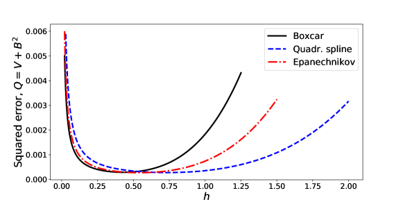
Figure 3: A sketch of the error, Eqs. (49), with $\rho(x)$ and $\rho^{\prime\prime}(x)^{2}$ averaged, as a function of $h$ for the boxcar, Epanechnikov and quadratic spline kernels, showing a slightly lower minimum at $h_{\rm opt}$ for the Epanechnikov. Also, note the higher values of $h_{\rm opt}$ and the broader minima for the Epanechnikov and quadratic spline kernels, in agreement with the results summarized in Table 2.

Next we illustrate how our results can be applied to algorithms of practical importance, i.e., including grid discretization.

5 Grid discretization

So far we have obtained results in continuous spatial variables. For numerical purposes, we need to perform grid discretization. Clearly, there is no universal discretization and different problems may benefit from different discretizations. For illustration purposes, in this section we choose a particular finite difference discretization that is commonly used in electrostatic PIC algorithms [8] but repeating the analysis for other discretizations is straightforward, including the use of finite elements.

5.1 Estimation kernel, particle shapes, and the sum rule

An important step in obtaining a complete particle algorithm is the connection of Lagrangian particles with a Eulerian grid. This connection is given by a charge deposition rule and traditionally done with so-called spline functions [8]. Although spline functions of varying degree of smoothness and width are available, they have the following two limitations: (i) their width is an integer number of cell widths, $i\Delta$, $i=1,2,\ldots$; and (ii) their width and smoothness are strictly related, with smoother particles being wider. The smoothness of a particle becomes important when force interpolation from the grid to the particle position, especially when a particle crosses cell boundaries. Since in this work we are not addressing the full PIC cycle, we emphasize the importance of particle width over smoothness. As well, if one were to use particles arbitrarily related to the grid spacing $\Delta$ to minimize noise and error, per our theoretical developments, the above restrictions may present a drawback. For example, when high grid resolution is desired (small $\Delta$) while $h_{\rm opt}$ is (relatively) large, that would require a particle that spans a large number of cells. If splines are used, they would be of high order and computationally expensive because of the larger number of floating point operations associated with high order polynomials. In fact, this is why practitioners rarely go beyond fourth order spline functions. The advantage of being able to choose separately particle smoothness and width becomes obvious.

In this section we address the relaxation of the two limitations discussed above, those associated with the smoothness and the width of particle shapes. The former was discussed in Ref. [12], where the smoothness of particle shapes was decoupled from its width. An example of a cubic particle shape depositing charge on three grid points (same as the quadratic spline) was given therein; by the same method, for example, one could devise a quadratic particle wider than three cells, etc. The key element that allows this generalization is the distinction between the kernel $K(x)$ and the particle shape (factor) $S(x)$, alluded to in Sec. 2. Therefore, before proceeding to address the limitation associated with the particle width, we return to a discussion of the difference between $K(x)$ and $S(x)$.

It is the sum rule property that distinguishes a kernel from a particle shape, see Eq. (9). We will require that a particle shape satisfies the sum rule, whereas we will not impose this requirement on a kernel. That property states that the sum of the fractions of the computational particle’s charge deposited on the grid sum exactly to the charge carried by the particle, and this is true at any (continuously varying) particle position $\xi$. As a consequence, the total charge of the system after being deposited on the grid is also conserved. For example, for density that integrates to unity on a uniform grid with spacing $\Delta$, we have $\int_{0}^{1}\!\rho_{e}(x)\,dx=\sum_{\mu=1}^{N_{p}}q_{\mu}=1\,.$ Consider the amount of charge a single particle deposits on the grid point $x_{i}$. We use a charge deposition rule based on a particle shape $S(x)$, which gives for the fraction of that charge $q_{\mu}\Delta S(x_{i}-\xi_{\mu})$. We find that the density on the grid point $x_{i}$ due to depositing the charge from all the particles is

$$\rho_{e}(x_{i})\equiv\rho_{e,i}=\sum_{\mu=1}^{N_{p}}q_{\mu}S(x_{i}-\xi_{\mu})\,.$$ (59)

For particles with equal charges, $q_{\mu}=1/N_{p}$, we obtain

$$\sum_{i=1}^{N_{g}}\Delta\,\rho_{e,i}=\sum_{i=1}^{N_{g}}\Delta\sum_{\mu=1}^{N_{p}}q_{\mu}S_{i}(\xi_{\mu})=\sum_{\mu=1}^{N_{p}}\frac{1}{N_{p}}\sum_{i=1}^{N_{g}}\Delta S_{i}(\xi_{\mu})=\sum_{\mu=1}^{N_{p}}\frac{1}{N_{p}}=1\,.$$ (60)

We have defined $S_{k}(\xi_{\mu})\equiv S(x_{k}-\xi_{\mu})$ and invoked the sum rule, Eq. (9). Thus, the sum rule implies that the total charge assigned to the grid is preserved. If a particle shape does not satisfy the sum rule (i.e. it obeys conditions (3)–(7) for a kernel but not the sum rule), the lack of exact charge conservation would allow $E(1)\neq E(0)$. Of course, the total charge of the system is always conserved as long as no association with a computational grid is made, as discussed in Sec. 2. Examples of particle shapes (satisfying the sum rule) are given in Table 3. The first three are familiar from Ref. [8]; the last (trapezoidal) particle shape is discussed below. The charge deposition on the grid point $x_{i}$, associated with each of the particles in Table 3, is found by the substitution $x=\xi_{\mu}-x_{i}$, for $i=1,2,\ldots,N_{g}$.

Particle shape	Definition
Boxcar (NGP)	$S_{B}(x)=\frac{1}{\Delta}\left\{\begin{tabular}[]{ll}$1$, $\left|\frac{x}{\Delta}\right|\leq\frac{1}{2}$\\[4.30554pt] $0$ otherwise\,.\end{tabular}\right.$
Linear spline	$S_{L}(x)=\frac{1}{\Delta}\left\{\begin{tabular}[]{ll}$1-\left|\frac{x}{\Delta}\right|$, $\left|\frac{x}{\Delta}\right|\leq 1$\\[4.30554pt] $0$ otherwise\,.\end{tabular}\right.$
Quadratic spline	$S_{Q}(x)=\frac{1}{\Delta}\left\{\begin{tabular}[]{ll}$\frac{3}{4}-\left(\frac{x}{\Delta}\right)^{2}$, $\left|\frac{x}{\Delta}\right|\leq 1/2$\\[4.30554pt] $\frac{1}{2}\left(\frac{3}{2}-\left|\frac{x}{\Delta}\right|\right)^{2}$, $1/2\leq\left|\frac{x}{\Delta}\right|\leq 3/2$\\[4.30554pt] $0$ otherwise\,.\end{tabular}\right.$
Trapezoidal	$S_{T}(x)=\frac{1}{\Delta}\left\{\begin{tabular}[]{ll}$\frac{1}{2}$, $\left|\frac{x}{\Delta}\right|\leq 1/2$\\[4.30554pt] $\frac{1}{2}\left(\frac{3}{2}-\left|\frac{x}{\Delta}\right|\right)$, $1/2\leq\left|\frac{x}{\Delta}\right|\leq 3/2$\\[4.30554pt] $0$ otherwise\,,\end{tabular}\right.$

Table 3: Examples of particle shapes. These shapes are similar to the kernels of Table 1 and Fig. 1, but have integer valued cell width and satisfy the sum rule, Eq. (9).

We now describe the generalization associated with particle width: a particle shape satisfying the sum rule (9) is not required to have a width equal to an integer number of grid cells. In fact, such a shape can have (almost – see below) completely arbitrary width relative to the grid. To see this, consider a known “primary” particle shape that satisfies properties (3)–(7) and the sum rule (9), say $S_{0}(x)$, with $\sum_{i}\Delta S_{0}(x_{i}-\xi)=1$ for any value of $\xi\in[0,1]$. Then for an arbitrary kernel $K(x)$ satisfying properties (3)–(7), we perform the convolution

$$S(x)=\int\!K(y)S_{0}(x-y)\,dy.$$ (61)

The so-obtained new particle shape $S(x)$ satisfies the normalization (3):

$$\int_{0}^{1}\!S(x)\,dx=\int\!K(y)\,dy\int\!S_{0}(x-y)\,dx=\int\!K(y)\,dy=1\,.$$ (62)

The sum rule (9) is also easily verified:

$$\sum_{i=1}^{N_{g}}\Delta S(x_{i})=\int\!K(y)\sum_{i}\Delta S_{0}(x_{i}-y)\,dy=\int\!K(y)\,dy=1\,.$$ (63)

It is easy to verify that properties Eq. (4)–(7) are inherited by $S(x)$ as well. The width of $S(x)$ equals to the sum of the widths of $S_{0}(x)$ and $K(x)$. The procedure just described allows a kernel $K(x)$ of arbitrary width; we conclude that this construction allows one to generate arbitrary width particle shapes satisfying the sum rule, including such that are non-integer number of cells wide. The only condition on the width of $S(x)$ is that it cannot be less than the width of $S_{0}(x)$, hence the qualifier “almost” above; this is usually not a limitation. We stress that if a particle shape $S(x)$ is obtained from a kernel $K(x)$ and another particle shape, $S_{0}(x)$, their functional forms are different (in addition to their widths being different).

We note that the convolution described by Eq. (61) is the easiest way to obtain a particle shape that satisfies the sum rule. However, this is a sufficient but not necessary condition. As well, choosing a familiar particle shape obeying the sum rule as a primary, $S_{0}$, is the easiest way to ensure $S(x)$ satisfies the sum rule; again, this choice is sufficient but not necessary. In other words, it is possible that other methods of obtaining particle shapes that satisfy the sum rule exist.

The examples in Table 3 satisfy the sum rule and can either be used as primary to obtain other particle shapes or directly in a simulation. In fact, all particles from Table 3 can in turn be obtained by the convolution formula (61) as follows: the boxcar shape is the convolution of itself with a delta-function kernel; the linear shape is the convolution of the boxcar shape with a boxcar kernel of width $\Delta$; the quadratic spline shape is the convolution of the boxcar shape with a linear kernel (tent function) of width $2\Delta$; and finally, the trapezoidal shape is the convolution of the boxcar shape and a boxcar kernel of width $2\Delta$.

An example of a particle shape that is non-integer number of cells wide is given next. Consider the convolution of the boxcar particle shape of width $\Delta$ from Table 3 with the boxcar kernel of width $\delta$ with $0\leq\delta\leq\Delta$,

$$K_{\delta}(x)= \frac{1}{\delta}\left\{\begin{tabular}[]{ll}$1$,&$\left|\frac{x}{\delta}\right|\leq\frac{1}{2}$\\[5.38193pt] $0$&otherwise\,.\end{tabular}\right.$$ (66)

The convolution formula (61) gives the following trapezoidal particle shape, of width $\Delta+\delta$:

$$S_{\Delta+\delta}(x)= \int\!\!K_{\delta}(y)S_{B}(x-y)\,dy$$

$$= \frac{1}{\Delta}\left\{\begin{tabular}[]{ll}$1$,&$0\leq|x|\leq\frac{\Delta-\delta}{2}$\\[5.38193pt] $\frac{1}{\delta}\frac{\Delta+\delta}{2}-|\frac{x}{\delta}|$,&$\frac{\Delta-\delta}{2}\leq|x|\leq\frac{\Delta+\delta}{2}$\\[5.38193pt] $0$,&otherwise\,.\end{tabular}\right.$$ (70)

The particle shape (70) transforms into the usual $\Delta$-wide boxcar shape in the limit $\delta\rightarrow 0$ and into the usual $2\Delta$-wide linear shape in the limit $\delta\rightarrow\Delta$. Note that $\int\!\!S_{\Delta+\delta}(x)\,dx=1$, as expected. The fractional width particle is illustrated in Fig. 4. The charge deposition rule is found by substitution of $\xi-x_{i}$ into (70), where $x_{i}$ is the nearest grid point to the particle position and $|\xi-x_{i}|\leq\Delta/2$. The result is given in Table 4 and the construction by means of a convolution assures that the sum rule is satisfied for arbitrary values of $\delta$.

We remark that the dependence of the particle shape (70) on the fractional width $\delta$ is not a scaling transformation via a fundamental kernel such as changing $h$ in (8). Instead, this is a parametric shape transformation (with parameter $\delta$). Nevertheless, changing the shape via $\delta$ also changes the support of $S_{\Delta+\delta}$ and provides another means of attaining the optimal width, $h_{\rm opt}=\Delta+\delta$.

The existence of the fractional width particle shape (70) was noted in Ref. [18] and has been previously known in particle hydrodynamics. Its derivation, however, has been based on area weighting arguments and not on the more general convolution method given by (61). Again, the fractional width trapezoidal shape (70) is not the same as the trapezoidal shape listed in Table 3.

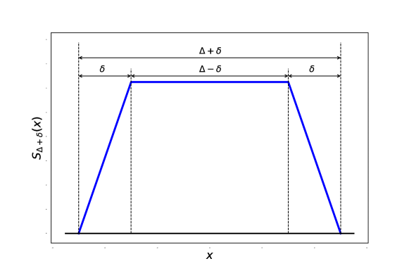
Figure 4: Illustration of the fractional width particle shape, Eq. (70), with $\delta/\Delta=0.4$ and $h=1.4\Delta$. Because this quantity is a convolution of two functions, one of which satisfies the sum rule in Eq. (9), it satisfies the sum rule for an arbitrary value of $\delta/\Delta$, and therefore for an arbitrary value of $h/\Delta<1$.

Charge deposition rule	Range
$S_{i-1}(\xi)=0$
$S_{i}(\xi)=\frac{1}{\Delta}$	$0\leq|\xi-x_{i}|\leq\frac{\Delta-\delta}{2}$
$S_{i+1}(\xi)=0$
$S_{i-1}(\xi)=\frac{1}{\Delta\delta}\left[-\frac{\Delta-\delta}{2}-(\xi-x_{i})\right]$
$S_{i}(\xi)=\frac{1}{\Delta\delta}\left[\frac{\Delta+\delta}{2}+(\xi-x_{i})\right]$	$-\frac{\Delta}{2}\leq\xi-x_{i}\leq-\frac{\Delta-\delta}{2}$
$S_{i+1}(\xi)=0$
$S_{i-1}(\xi)=0$
$S_{i}(\xi)=\frac{1}{\Delta\delta}\left[\frac{\Delta+\delta}{2}-(\xi-x_{i})\right]$	$\frac{\Delta-\delta}{2}\leq\xi-x_{i}\leq\frac{\Delta}{2}$
$S_{i+1}(\xi)=\frac{1}{\Delta\delta}\left[-\frac{\Delta-\delta}{2}+(\xi-x_{i})\right]$

Table 4: Charge deposition rule corresponding to the fractional particle shape (70).

Another approach to obtaining particle shapes of arbitrary support is based on the finite element method of discretizing a system of equations [34]. In particular, in particle algorithms based on a variational principle [4, 12], the convolution method of obtaining particle shapes emerges naturally [12] and the role of the above primary particle shape $S_{0}$, which provides the connection to the grid, is taken by finite element basis functions. For example, tent functions of width $2\Delta$ and height $1$ (linear Lagrange finite elements, which are basically the same as the linear spline shape function in Table 3 except with a different amplitude), $\Psi_{i}(x)=\Psi(\xi-x_{i})$, have the property that at any $x$ (including at grid points $x_{i}$)

$$\sum_{i=1}^{N_{g}}\Psi_{i}(x)=1\,.$$ (71)

Except for a factor $\Delta$, this is the sum rule that we require of particle shapes. That is, to obtain a particle shape $S(x)$ satisfying the sum rule (9), we perform the convolution $S(x)=\int_{0}^{1}\!K(y)\Psi(x-y)\,dy/\Delta$ with the finite element. (Note that translation invariance is also satisfied). The unit normalization follows from the finite element property $\int_{0}^{1}\!(1/\Delta)\Psi_{i}(x)\,dx=1$, $i=1,2,\ldots,N_{g}$, and the kernel normalization (3). The shapes (top to bottom) from Table 3 may also be obtained by the finite element method from convolutions.

To summarize, relaxing the limitations associated with particle smoothness and width allows one to devise particle shapes that are both computationally efficient and suitable to take advantage of the BVO guidelines discussed in the previous section, as well as assuring that the sum rule is satisfied.

5.2 Density analysis in discrete variables

We consider a uniform grid in $x$ on $[0,1]$ with vertices at $x_{i}=\Delta i$, $i=0,\cdots,N_{g}$ and grid spacing $\Delta=1/N_{g}$. Returning to $\rho(x)=1$ for simplicity, we define the estimated density at cell centers, $x_{i+1/2}=(i+1/2)\Delta$, as

$$\rho_{e,i+1/2}=\rho_{e}(x_{i+1/2}),\quad 0\leq i\leq N_{g}-1\,.$$

Note that given a particle shape, e.g., from Table 3, charge deposition on cell centers amounts to simply substituting $x=\xi-x_{i+1/2}$ in $S(x)$. Recall that for uniform density we have $\langle\rho_{e,i+1/2}\rangle\equiv\left<\rho_{e}(x_{i+1/2})\right>=1$; then the discrete approximation to $\int\rho_{e}(x)dx=1$ is

$$\sum_{i=0}^{N_{g}-1}\rho_{e,i+1/2}\Delta=\sum_{i,\mu}q_{\mu}S_{i+1/2}(\xi_{\mu})\Delta=\sum_{\mu}q_{\mu}\sum_{i}\Delta S(x_{i+1/2}-\xi_{\mu})=1.$$ (72)

For the covariance matrix we have, from Eqs. (19), (21)

$$C_{i+1/2,j+1/2}\equiv C(x_{i+1/2},x_{j+1/2})=C_{d,i+1/2,j+1/2}-\frac{1}{N_{p}}$$

$$=\frac{1}{N_{p}}\left[\int S(x_{i+1/2}-\xi)S(x_{j+1/2}-\xi)d\xi-1\right],$$ (73)

the last equality due to the sum rule, Eq. (9), and $\sum_{\mu}q_{\mu}=1$. The discrete analog of Eq. (23) is the condition that the sum over each row (or column) of the covariance matrix is zero; we have

$$\sum_{j}\Delta C_{i+1/2,j+1/2}= \frac{1}{N_{p}}\left[\sum_{j}\Delta\int S(x_{i+1/2}-\xi)S(x_{j+1/2}-\xi)d\xi-1\right]$$

$$= \frac{1}{N_{p}}\left[\Delta\sum_{j}\hat{S}(x_{i+1/2}-x_{j+1/2})-1\right]=0\,,$$ (74)

where $\hat{S}$ is the convolution of $S$ with itself. Since $S$ satisfies the sum rule and assumptions (3)–(7), so does $\hat{S}$, therefore, the quantity in Eq. (74) sums to zero and we obtain the analogous discrete result as in Eq. (23). As in the continuous case, this identity says that the vector $u_{i}=1$ is associated with zero eigenvalue, implying that the covariance matrix is singular. In the next section we will show exact calculations of these covariance matrix elements for specific particle shapes.

The negative correlations of Eq. (21) also appear in Eq. (73). In order to understand these correlations, let us compare a case in which we pick the number $N_{i+1/2}$ of particles in the cells independently and identically distributed (iid) from a Poisson distribution with parameter $\lambda=N_{ppc}=N_{p}\Delta$, with mean $\lambda$ and variance $\lambda$. Here, $N_{ppc}$ is the expected number of particles per cell. Again, recall that in this discussion, we are assuming $\rho(x)=1$; thus the mean of $\rho_{e,i+1/2}=N_{i+1/2}/N_{ppc}$ is unity and its variance is $1/N_{ppc}$. Indeed, from the iid assumption, the off-diagonal terms are zero and using the property of the variance, $\mbox{Var}(\rho_{e,i+1/2})=\mbox{Var}(N_{1+1/2})/N_{ppc}^{2}$, we obtain

$$C_{i+1/2,j+1/2}=\frac{\lambda}{N_{ppc}^{2}}\delta_{ij}=\frac{1}{N_{ppc}}\delta_{ij}.$$ (75)

Referring to Eqs. (8), (73), for a kernel of width $h\sim\Delta$, the diagonal (the variance) is $\sim 1/\Delta N_{p}=1/N_{ppc}$, comparable to the dominant part of the diagonal in Eqs. (73), (74). However, the negative correlations $-1/N_{p}$ in Eqs. (21) and (73) are not contained in the Poisson model. These negative correlations are traced to the fact that the total number of particles $N_{p}$ in Eqs. (21) and (73) is fixed. In a particle code, the total number of particles can be assumed fixed at each time step. (The particle number may also be constant throughout the simulation for certain type of boundary conditions such as periodic, for example.) The fixed number of particles is in contrast to the Poisson case in which the expected number of particles per cell is $N_{ppc}$ (expected total number of particles $=N_{p}$). Intuitively, when the total number of particles is fixed, if one cell has more than the expected number of particles $N_{ppc}$, other cells must necessarily have fewer particles, leading to negative correlations. (See also Ref. [35] where negative correlations between numbers of particles in different cells were obtained working from the multinomial distribution.) We will discuss in a later section the effect of these negative correlations on the calculation of the electric field.

5.3 Covariance $C_{i+1/2,j+1/2}$ examples

In this section we present covariance matrix calculations with particle shapes from Table 3. The simplest particle shape is the boxcar (top-hat) function. For $i\neq j$ the overlap integral in Eq. (73) is zero and we find

$$C_{i+1/2,j+1/2}=-\frac{1}{N_{p}}\,\,\,(j\neq i)$$

giving

$$C_{i+1/2,j+1/2}=\frac{1}{N_{ppc}}\delta_{ij}-\frac{1}{N_{p}}.$$ (76)

The first term in Eq. (76) is equal to the value in Eq. (75), and the second term is recognized as the negative term of Eq. (73). We conclude indeed that the $-1/N_{p}$ term is due to the fact that the total number of particles is fixed. The condition (74) is obviously satisfied in this example.

For the linear particle shape we find

$$C_{i+1/2,j+1/2}=\left\{\begin{tabular}[]{ll}$\frac{1}{N_{p}}\left[\Delta\int S(\xi)^{2}d\xi-1\right]=\frac{1}{N_{p}}\left[\frac{2}{3\Delta}-1\right]=\frac{2}{3N_{ppc}}-\frac{1}{N_{p}}\,\,\,$&$(j=i)$,\\ \rule{0.0pt}{17.22217pt} $\frac{1}{N_{p}}\left[\Delta\int S(\xi-1)S(\xi)d\xi-1\right]=\frac{1}{6N_{ppc}}-\frac{1}{N_{p}}\,\,\,$&$(j=i\pm 1)$,\\ \rule{0.0pt}{17.22217pt} $-\frac{1}{N_{p}}\,\,\,$&\mbox{otherwise}.\end{tabular}\right.$$ (77)

Note that the condition (74) holds for this example as well. This condition highlights the importance of the $-1/N_{p}$ correlations and shows how the variances ($i=j$ terms) decrease as the particle width increases.

For the quadratic particle shape we have

$$C_{i+1/2,j+1/2}=\left\{\begin{tabular}[]{ll}$\frac{11}{20N_{ppc}}-\frac{1}{N_{p}}\,\,\,$&$(j=i)$\\ \rule{0.0pt}{12.91663pt} $\frac{13}{60N_{ppc}}-\frac{1}{N_{p}}\,\,\,$&$(j=i\pm 1)$\\ \rule{0.0pt}{12.91663pt} $\frac{1}{120N_{ppc}}-\frac{1}{N_{p}}\,\,\,$&$(j=i\pm 2)$\\ \rule{0.0pt}{12.91663pt} $-\frac{1}{N_{p}}\,\,\,$&\mbox{otherwise}.\end{tabular}\right.$$ (78)

The property (74) is again clearly seen for all these cases. Note again that the variances, i.e. the $i=j$ terms, decrease further as the particle widths increase, with their values distributed to more neighboring bands, with the negative term $-1/N_{p}$ on diagonal as well as off-diagonal terms.

5.4 Discretized electric field correlations

In this section we analyze the statistical properties of the electric field on a grid, again assuming uniform density, $\rho(x)=1$. The continuous form of these relations was presented in Sec. 3.2. In the previous section, the density was assumed to reside at cell centers $\rho_{e,i+1/2}$, i.e., at $x_{i+1/2}$. If the density and the electric field are taken to be staggered, with $E_{i}$ residing at vertices $x_{i}$ for $i=0,\cdots,N_{g}$, to obtain a second order accurate differencing scheme, we write

$$E_{i+1}-E_{i}=\Delta\rho_{q,i+1/2},$$ (79)

where $\rho_{q,i+1/2}=1-\rho_{e,i+1/2}$ is the charge density and, as before, assuming uniform and immobile ions of unit (neutralizing) density. This relation leads to $E_{i}=E_{0}+E_{1,i}$, where

$$E_{1,i}=\Delta\sum_{j=0}^{i-1}\rho_{q,j+1/2}.$$ (80)

The condition $E_{0}=E_{N_{g}}$ ($x_{0}=0,\,\,x_{N_{g}}=1$) follows from

$$\sum_{j=0}^{N_{g}-1}\rho_{q,i+1/2}=0$$ (81)

and Eq. (72). (It is instructive to revisit the derivation of the discrete property (74): this result can be obtained directly by writing $\sum_{j}\langle\tilde{\rho}_{e,i+1/2}\tilde{\rho}_{e,j+1/2}\rangle$ $=\langle\tilde{\rho}_{q,i+1/2}\sum_{j}\tilde{\rho}_{q,j+1/2}\rangle$, which is seen to vanish by Eq. (81).) The condition in Eq. (25) of having zero applied potential across a period takes the discrete form

$$\sum_{i=0}^{N_{g}-1}\Delta E_{i}=\Delta N_{g}E_{0}+\sum_{i=1}^{N_{g}-1}E_{1,i}=0.$$ (82)

This is a condition on $E_{0}$; we find

$$E_{0}= -\Delta^{2}\sum_{i=0}^{N_{g}-1}\sum_{j=0}^{i-1}\rho_{q,j+1/2}$$

$$= -\Delta^{2}\sum_{j=0}^{N_{g}-2}(N_{g}-j-1)\rho_{q,j+1/2}.$$

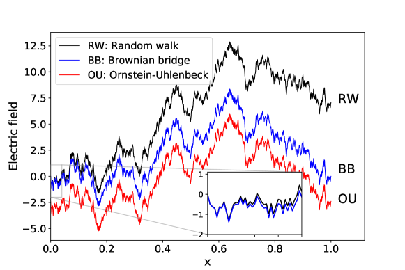
Figure 5: Illustration of three types of random behavior of the electric field depending on the boundary conditions, as discussed in Appendix A. Both RW and BB have a starting point $E(0)=0$ (see inset); the BB case has additionally $E(1)=0$, and the OU case is shifted down, satisfying the zero potential difference condition.

As in Sec. 3.2, the terms in Eq. (80) lead to four distinct terms in the covariance matrix for the noise in the electric field, $\langle\tilde{E}_{i}\tilde{E}_{j}\rangle=C_{00}^{E}+C_{10,i}^{E}+C_{01,j}^{E}+C_{11,ij}^{E}$, where

$$C_{00}^{E}=\langle\tilde{E}_{0}^{2}\rangle,$$ (83)

$$C_{10,i}^{E}=\langle\tilde{E}_{1,i}\tilde{E}_{0}\rangle,$$ (84)

similarly for $C_{01,j}^{E}$, and

$$C_{11,ij}^{E}=\langle\tilde{E}_{1,i}\tilde{E}_{1,j}\rangle.$$ (85)

For the first of these we find

$$C_{00}^{E}=\Delta^{4}\sum_{j=0}^{N_{g}-2}(N_{g}-j-1)\sum_{k=0}^{N_{g}-2}(N_{g}-k-1)C_{j+1/2,k+1/2},$$ (86)

where $C_{j+1/2,k+1/2}=\langle\tilde{\rho}_{q,j+1/2}\tilde{\rho}_{q,k+1/2}\rangle.$ For the next term (and similarly for $C_{01,j}^{E}$) we have

$$C_{10,i}^{E}=-\Delta^{3}\sum_{j=0}^{i-1}\sum_{k=0}^{N_{g}-2}(N_{g}-k-1)C_{j+1/2,k+1/2}.$$ (87)

Finally, the last term is

$$C_{11,ij}^{E}=\Delta^{2}\sum_{k=0}^{i-1}\sum_{l=0}^{j-1}C_{k+1/2,l+1/2}.$$ (88)

For this covariance matrix we find

$$C_{11,ij}^{E}=\frac{1}{N_{p}}\left(\Delta\min(i,j)-\Delta^{2}ij\right)=\frac{1}{N_{p}}\left(\min(x_{i},x_{j})-x_{i}x_{j}\right).$$

The first term is the value for the Poisson case and the second is the Brownian bridge contribution from the constant correlations $-1/N_{p}$ in Eq. (76). The remaining terms arise from the Ornstein-Uhlenbeck bridge; we have

$$C_{10,i}^{E}=\frac{1}{N_{p}}\left(-\Delta^{2}(N_{g}-1)i+\frac{\Delta^{2}i(i-1)}{2}+\frac{\Delta^{3}N_{g}(N_{g}-1)i}{2}\right)$$

$$\rightarrow\frac{1}{N_{p}}\left(\frac{x_{i}^{2}}{2}-\frac{x_{i}}{2}\right),$$

the latter limit as $\Delta\rightarrow 0$ with $\Delta N_{g}$=1. The quantity $C_{01,j}^{E}$ is computed similarly and

$$C_{00}^{E}=\frac{1}{N_{p}}\left(\Delta^{3}\frac{(N_{g}-1)N_{g}(2N_{g}-1)}{6}-\Delta^{4}\frac{N_{g}^{2}(N_{g}-1)^{2}}{4}\right)$$

$$\rightarrow\frac{1}{12N_{p}}$$

and in the same limit, $\Delta\rightarrow 0$. We see that the limiting case is in agreement with Eq. (33).

The three different types of random behavior of the electric field, depending on the boundary conditions, is illustrated in Fig. 5. The random walk curve is a Brownian motion with $E(0)=0$ without imposing any boundary condition at $x=1$, the Brownian bridge curve reflects the extra boundary condition $E(0)=E(1)=0$, and the Ornstein-Uhlenbeck curve satisfies both $E(0)=E(1)=0$ and the zero potential difference condition. The latter means that if $E(x)$ makes an excursion into the positive half plane, it must do so in negative half plane as well so that $E(x)$ integrates to zero – see the discussion in terms of position, velocity, and acceleration in Appendix A.

In the next section we verify numerically our theoretical conclusions.

6 Numerical results

Considerations dictating the choice of a charge deposition rule in a particle algorithm were discussed in Sec. 5.1, where two important factors were identified – smoothness and width. In sections 3 and 4 we have found the particle width to be more relevant to our discussion: it reduces the variance for uniform density and minimizes the error in a non-uniform density via the BVO process, independent of grid resolution. For discretization on a grid, we have also emphasized the importance of obeying the sum rule.

One strategy for applying our theory in practice is to use particles that have width closest to the optimal, i.e., $h=i\Delta+\delta\approx h_{\rm opt}$ with $h_{\rm opt}$ given by (52), $i$ an integer number, and $\Delta$ chosen according to a desired grid resolution. One may further decide on a particle that is an integer number of cells wide or add the additional correction $\delta$. Using particles with exact width equal to $h_{\rm opt}$ is obviously not possible in general simulations where the exact density and its gradients are unknown and may vary in time. However, the estimated quantities can be used as a guideline or a lower resolution simulation may be done to probe for these and other properties of a physical system. As discussed previously, spline functions of order $i>4$ are probably not the most efficient choice and custom particles may be better suited. If one uses high grid resolution (small $\Delta$), one may be able to approximate $h_{\rm opt}$ sufficiently well with an integer number of cells, $h=i\Delta\approx h_{\rm opt}$; However, one advantage of using a fractional width shape with a correction $\delta$ is that the same charge deposition can be used and adjusted “in real time,” depending on the values of $\rho(x)$ and $\rho^{\prime\prime}(x)$. This provides “fine tuning” ability, which may be preferable to changing the type/width of particle in the course of a simulation and may help to avoid introducing undesired effects or difficulties.

In the following sections, our focus will be on theory comparison and verification, which is why we will not be concerned with the requirement of grid resolution. Instead, we will use the grid spacing to adjust the width of the same particle shape, thus applying the scaling transform $K(x)=K_{f}(x/h)/h$. When using the scaling method, we will not be dealing with fractional width particles; therefore, to change the width of a given particle, we will vary the grid spacing by integer numbers: for example, when $N_{g}=15$, the width of the three-cell-wide quadratic spline equals $h=3\Delta=3/15=0.2$, for $N_{g}=30$ its width equals $h=3/30=0.1$, etc. Recall that we work in the domain $[0,1]$; a range of $N_{g}\simeq 15\ldots 50$ will prove to provide a sufficient range of particle widths. In a separate set of simulations, we present results on a fixed grid but varying the fractional width of the particle defined in (70).

6.1 Covariance matrix in uniform density

We present as a first example numerical computations of the density covariance matrix with uniform true density $\rho(x)=1$ on a uniform periodic grid on $[0,1]$ and we use the linear particle shape from Table 3 for our charge deposition. Recall that the covariance matrix for this case is given by Eq. (77); however, more convenient quantities to test are the products

$$\widetilde{C}_{i+\frac{1}{2},i+\frac{1}{2}}\equiv C_{i+\frac{1}{2},i+\frac{1}{2}}\times N_{ppc} =\frac{2}{3}-\Delta\,,$$ (89)

$$\widetilde{C}_{i+\frac{1}{2},i+\frac{1}{2}\pm 1}\equiv C_{i+\frac{1}{2},i+\frac{1}{2}\pm 1}\times N_{ppc} =\frac{1}{6}-\Delta$$ (90)

since they are independent of $N_{ppc}$ and $N_{p}$.

The theory was developed in the limit of infinite number of samples by integrating over a continuous density distribution but clearly, numerically we can only use a finite number of samples in averages. The present results aim to verify the developed theory as well as to inform us of the number of samples needed in simulations in the next section. Because in this section we deal with uniform density, the correlations are expected to be the same for every grid point. Using this fact, we can obtain better statistics by averaging correlations over the whole grid, i.e., $\bar{C}_{i+\frac{1}{2},i+\frac{1}{2}}=(1/N_{g})\sum_{1}^{N_{g}}C_{i+\frac{1}{2},i+\frac{1}{2}}$ for every $i=1\ldots N_{g}$. Therefore, for a number of $M_{\rm local}$ samples, such averaging amounts to performing $M=N_{g}\times M_{\rm local}$ local cell samples; to the end of this section we omit the over-bar. Each particle sample is drawn from a uniform distribution by drawing $N_{p}$ random numbers $R\in[0,1]$ and setting particle positions $\xi_{\mu}=R$, $\mu=1,2,\ldots N_{p}$.

Simulation results on a fixed grid with $N_{g}=25$ ($\Delta=0.04$) are listed in Table 5. Theory predicts $\widetilde{C}_{i+\frac{1}{2},i+\frac{1}{2}}=0.666\ldots-0.04=0.6266\ldots$ and $\widetilde{C}_{i+\frac{1}{2},i+\frac{1}{2}\pm 1}=0.1666\ldots-0.04=0.1266\ldots$.

$N_{p}$	$M$	$\widetilde{C}_{i+\frac{1}{2},i+\frac{1}{2}}$		$\widetilde{C}_{i+\frac{1}{2},i+\frac{1}{2}\pm 1}$
		theoretical	numerical	theoretical	numerical
250	$2.5\times 10^{6}$	0.6266…	0.6269	0.1266…	0.1267
2500	$2.5\times 10^{5}$		0.6256		0.1251
25,000	$2.5\times 10^{4}$		0.6208		0.1252

Table 5: Simulation results for uniform density distribution. The theoretical values have the fixed quantity $\Delta$ subtracted. In the numerical values, this quantity is not subtracted explicitly.

We have also intentionally taken the product $N_{p}\times M=\mbox{const.}$ in order to examine the role of number of samples versus number of particles. The numerical values in the table agree with the theoretical values of the correlations and are most accurate (to $3$ significant figures) when using the largest number of samples $M=2.5\times 10^{6}$ – the first row in Table 5. Using a larger number of particles and smaller number of samples shows good agreement as well, albeit with a somewhat larger error in the third significant figure. We conclude that a number of samples of order $10^{6}$ should be sufficient for comparison with theory, with three significant figures and a small error bar in the third significant figure.

6.2 Bias-variance optimization in non-uniform density

This set of simulations aims to compare numerical results and theory for the local error in a non-uniform density, $\rho(x)\neq\mbox{const.}$ We compare the minimum error and optimal particle width for four different shapes, all having the same support $h=3\Delta$: the boxcar shape scaled to $3\Delta$, the quadratic spline and the trapezoidal shape from Table 3, and the Epanechnikov kernel scaled to $3\Delta$,

$$K_{E}(x)=\frac{1}{\Delta}\left\{\begin{tabular}[]{ll}$\frac{1}{2}\left(1-\frac{4}{9}\left(\frac{x}{\Delta}\right)^{2}\right),$&$\left|\frac{x}{\Delta}\right|\leq\frac{3}{2}$\\[5.38193pt] $0$&otherwise\,.\end{tabular}\right.$$ (91)

These four shapes also have different smoothness, which is another point of comparison. We note that the wider boxcar shape satisfies the sum rule just as the $\Delta$-wide NGP shape does but deposits constant amount of charge on three grid points instead of one. Unlike the first three shapes, the Epanechnikov kernel (91) does not satisfy the sum rule and therefore does not conserve charge on the grid, i.e., is not a particle shape in the sense of Sec. 5.1. For this reason, the Epanechnikov kernel is not recommended for practical applications; however, for our purpose of statistical calculations, charge conservation is not required. The trapezoidal shape (which does satisfy the sum rule) is also unusual and since we have not tested it in full particle simulations, we do not recommend it for practical use at this point. The purpose of present comparisons is to (i) verify the theoretical prediction that the minimal error depends primarily on the particle width and not significantly on the specific particle shape (and smoothness); and (ii) to verify the general dependence of $Q_{\rm min}$ and $h_{\rm opt}$ on the particle shape.

For all simulations in this section the true density distribution is given by the periodic function

$$\rho(x)=1+a\cos(2\pi mx)\,,$$ (92)

where $a<1$ is a constant amplitude and $m$ is an integer mode number. Since (92) satisfies $\int_{0}^{1}\rho(x)\,dx=1$ and $\rho(x)\geq 0$ for $x\in[0,1]$, it is a probability density distribution. For all simulations in this section we have chosen $a=1/2$, and $m=2$. We show results for two locations: $x=1/2$, where $\rho(1/2)=3/2$ and $\rho^{\prime\prime}(1/2)=-8\pi^{2}$, and $x=1/3$, where $\rho(1/3)=3/4$ and $\rho^{\prime\prime}(1/3)=-4\pi^{2}$. The number of samples is $M=10^{6}$ and the number of particles is $N_{p}=10^{4}$, unless otherwise stated. Drawing a sample from the density (92) was done by by the transformation method [36], by which the cumulative distribution function of $\rho(x)$ is inverted; this process is repeated $\mu=1\ldots N_{p}$ times for the particles in the sample. The whole process is repeated for a total of $M$ samples. We note that by connecting particle widths to integer number of cells, we do not reach the absolute theoretical minimum $h_{\rm opt}$ since $N_{g}$ in a domain of fixed size can only be an integer number and $\Delta=1/N_{g}$ can only take discrete values.

Before discussing the numerical simulations, let us look qualitatively at the error minimum for the density (92), based on the order of magnitude estimates (50). We assume the kernel width is a multiple of the grid spacing and for simplicity take $h=\Delta$, i.e., we estimate the density with a boxcar shape. Using the scaling transformation (8), we vary the grid in the range $N_{g}\in[16,48]$, which corresponds to kernel widths in the range $h\in[0.02083,0.0625]$. We need to compare $h$ with, the density gradient scale length, which for our case of Eq. (92) at $x=1/2$ gives $l=\sqrt{1.5/8\pi^{2}}\simeq 0.138$. The qualitative bias and variance error curves are illustrated in Fig. 6, showing that we should expect a minimum in this range of simulation parameters. Notice that the lowest value of $h$ corresponds to $N_{g}=48$ and is an acceptable grid resolution for our cosine density profile, having $24$ grid points per period; it does not, however, correspond to $h_{\rm opt}$, the error being about $50\%$ above the actual minimum. If we were to set up a grid corresponding to $h_{\rm opt}$ (using the same particle, with $h=\Delta$), it would correspond to $N_{g}\simeq 32$ and we would be somewhat under-resolving the cosine period with only about $16$ grid points per period. We shall not further discuss this issue but emphasize that grid resolution is a factor that must be chosen based on grid truncation errors and independently from the particle shape, whose width is chosen to minimize $Q=V+B^{2}$, where the variance $V$ is a measure of the statistical error. Finally, the quantity $N_{h}$ from Eq. (51) is equivalent to the number of particles per cell, $N_{ppc}$, in the discretized system. For a total of $N_{p}=10^{4}$ particles, we find $N_{ppc}\in[312,937]$ for $N_{g}\in[16,48]$, and $N_{ppc}\simeq 450$ at the intersection of the two curves, which is close to the minimum of $Q=V+B^{2}$. Note that in the intersection region the bias curve depends more strongly on $h$ than the variance curve, suggesting that a more efficient way to “locate” (and follow) the minimum of the error curve is by adjusting $h$ rather than by adjusting the number of particles in a simulation. One should keep in mind that the exact numerical parameters discussed above may differ from the exact figures by a factor of a few, coming from the shape coefficients $C_{1}$ and $C_{2}$, which were not included in the estimates (50) and (51).

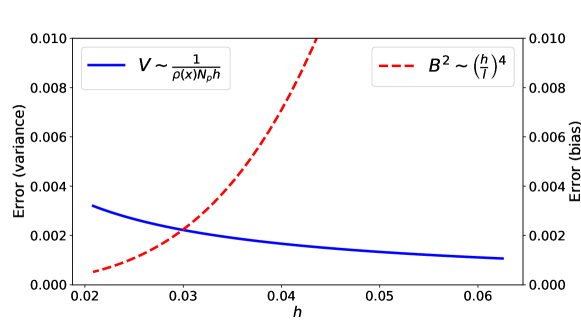
Figure 6: Qualitative comparison of the terms representing the bias and variance errors in Eq. (50).

Numerical results for the above setup are shown in Fig. 7 at the location $x=1/2$. In this simulation we use the scaling transform, Eq. (8), which is accomplished by changing the grid spacing $\Delta$ (or $N_{g}$) and thus the particle width $h=3\Delta=3/N_{g}$. In the figure each point corresponds to a different $N_{g}$ but we remind the reader that the grid resolution is irrelevant to BVO calculations and thus we should not expect interference with the results for $h_{\rm opt}$ and $Q_{\rm min}$. As predicted by theory, a minimum of the error is achieved at some value $h_{\rm opt}$. Further, the value of the minimal error changes very little between the four different shapes. The value of $h_{\rm opt}$ is seen to vary, with the exception of the trapezoidal shape and the Epanechnikov kernel, which show similar values for both $h_{\rm opt}$ and $Q_{\rm min}$. To understand the similarities and differences better, we use the values of the constants $C_{1}$ and $C_{2}$ from Table 2 to calculate the theoretical $Q_{\rm min}$ and $h_{\rm opt}$ from Eqs. (52) and (53). The results in Table 6 confirm our observations and also show good agreement between theoretical and numerical calculations.

One important point concerning comparisons between numerical and theoretical results should be made. The theoretical calculations involved certain approximations such as termination of the Taylor expansion in Eq. (41) and neglecting terms $\sim 1/N_{p}$ in Eq. (44). In contrast, the numerical results are in this sense “exact” since no approximations are made; the only inaccuracy in the numerical results stems from the finite number of samples used in the averages. It is plausible that certain density profiles may require keeping some of the other neglected terms to better describe the optimal width and error. This situation may occur, for example, when at isolated locations, $x_{0}$, the second derivative of the density vanishes, $\rho^{\prime\prime}(x_{0})=0$. Such occurrences are exceptions rather than the general situation and of course, the averaged theory, Eqs. (55), (56), remains unaffected. For the density profile (92) we will see below that at the specified above spatial locations, including one extra term in the theoretical calculations further improves the agreement by a few percent.

In Figure 8 we show comparison between local theory, Eqs. (52), (53), averaged theory, Eqs. (55), (56), and simulations for the two locations, $x=1/3$ (top panel) and $x=1/2$ (bottom panel), for the same quadratic spline particle shape (cf. Table 3). The lines labeled “Theory (local)” are plots of formula (49); the lines labeled “Theory (average)” are plots of the integrated (from $0$ to $1$) Eq. (49). Both theory and averaged theory use the values of $C_{1}$ and $C_{2}$ from Table 2. We see that the averaged theory does not change between the top and bottom panels since $h_{\rm opt}$ and $Q_{\rm min}$ do not depend on $x$. (The apparent difference is due to the slightly different plotting range.) In order to obtain even better agreement between local theory and simulations, we have included the small correction $-\rho(x)^{2}/N_{p}$ in Eq. (44), which has been neglected so far; that yields an improvement of about $5\%$. Including that term also explains the slight difference in the theoretical values of $h_{\rm opt}$ and $Q_{\rm min}$ that the discerning eye would observe in the legend of Fig. 8 (bottom panel) versus the table values in Table 6 (Quadr. spline).

Lastly, we present simulations of bias-variance optimization with the fractional width particle shape, Eq. (70). Recall that the fractional particle shape is not a simple scaling transform as the cases considered thus far but is a shape transform, which additionally changes the measure of its support. The theory developed in Sec. 4 was for a scaling transform only, keeping the particle shape unchanged. Therefore that theory cannot be used for quantitative comparison with the following simulations but can nevertheless serve as a guideline to understanding the numerically observed behavior of $Q_{\rm min}$ and $h_{\rm opt}$.

These simulations were performed at $x=1/2$, for two fixed grid sizes, $N_{g}=8$ and $16$, with $N_{p}=1000$. The smaller number of particles was chosen to increase (for clarity) the relative numerical error due to the finite number of samples: for $1000$ particles, the value of $Q_{\rm min}$ is expected to be about $10^{4/5}\approx 6.31$ times larger while the value of $h_{\rm opt}$ to be about $10^{1/5}\approx 1.58$ times larger. As a guideline for the values of the minimal error and optimal width, we take the averages of $Q_{\rm min}$ and $h_{\rm opt}$ between the two limiting shapes ($\Delta$-wide boxcar and $2\Delta$-wide linear tent); these average values are $Q_{\rm min}\sim 0.0143$ and $h_{\rm opt}\sim 0.154$. The simulation results in Fig. 9 show minimum error $Q_{\rm min}\approx 0.0113$ and optimal width $h_{\rm opt}\approx 0.17$, consistent with the above predictions. The observed discontinuity in the $Q(h)$ curve is also expected and easy to explain. For the range $0.0625<h<0.125$ we use $\Delta=0.0625$ (or $N_{g}=16$), and for $0.125<h<0.250$, we use $\Delta=0.125$ (or $N_{g}=8$). The fractional width particle becomes a $\Delta$-wide boxcar shape for $\delta=0$ and a $2\Delta$-wide linear shape for $\delta=\Delta$. Therefore, on the left side of the discontinuity the density is estimated by a linear particle shape of width $0.125$ while on the right it is estimated by a boxcar shape of the same width. Estimating the density by two different shapes (of the same width) is expected to produce different errors $Q$ because of the different values of the shape coefficients $C_{1}$ and $C_{2}$ (see Table 2).

From the results in Fig. 9 we conclude that the fractional width particle shape can indeed be used to attain the BVO minimum error without having to change the type of particle (or charge deposition rule).

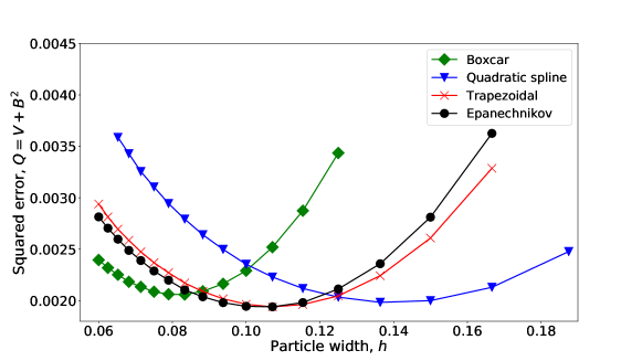
Figure 7: Local bias-variance optimization comparison of four different shapes at $x=1/2$, from numerical computations. Although the value of $h_{\rm opt}$ changes noticeably between the different shapes, the value of $Q_{\rm min}$ depends little on the shape of the particle, in agreement with the results summarized in Table 2.

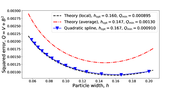
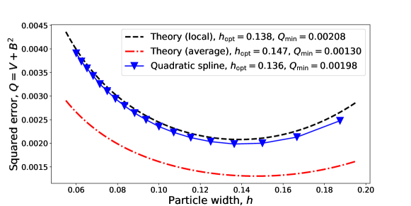
Figure 8: Bias-variance optimization comparison between exact local theory, averaged theory, and simulations for the quadratic spline particle shape. Top panel: $x=1/3$. Bottom panel: $x=1/2$.

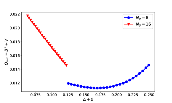
Figure 9: Local bias-variance optimization at $x=1/2$ with the fractional width particle (70). The particle width $h=\Delta+\delta$ varies by changing $\delta$, but at the step discontinuity you have to change both $\delta$ and $\Delta$. (See the text.)

Shape	$Q_{\rm min}$		$h_{\rm opt}$
	theoretical	numerical	theoretical	numerical
Boxcar	$0.00232$	$0.00206$	$0.0810$	$0.0833$
Quadr. spline	$0.00223$	$0.00198$	$0.139$	$0.136$
Trapezoidal	$0.00219$	$0.00194$	$0.107$	$0.107$
Epanechnikov	$0.00219$	$0.00194$	$0.103$	$0.107$

Table 6: Comparison of theoretical values, Eqs. (52) and (53), and numerical values of the optimal particle width and the error minimum. The more accurate value $Q_{\rm min}=0.002186$ of the minimal error for Epanechnikov kernel is indeed slightly lower than the value of the trapezoidal shape; the table entry has been rounded off to three significant figures.

7 Summary and conclusions

We have presented analyses of the noise in particle methods used to study electrostatic models in one dimension. We have described kernel density estimation for continuous $x$, expressing the kernel in terms of a fundamental kernel $K_{f}$ of width $1$, namely $K(x)=(1/h)K_{f}(x/h)$. In this form its shape ($K_{f}$) and its width $h$ are represented separately. Restricting our attention to uniform true electron density $\rho(x)$ for these initial studies (and immobile ions of uniform, fixed density $\rho_{i}(x)$ throughout the paper), we have computed the covariance matrix $C(x,y)$ of the noise in the estimated electron density $\rho_{e}(x)$. There are positive off-diagonal elements of the covariance matrix related to the width $h$ of the kernel. But, more importantly, there are constant negative elements, on and off the diagonal (the latter related to negative correlations). These negative matrix elements arise from the fact that the total number of particles is fixed at each time step. That is, for example, if the particles are concentrated in one area (higher density estimate), they will be necessarily more sparse (lower density estimate) in other areas. These negative correlations lead to the property $\int\!C(x,y)dy=0$, i.e. $C(x,y)$ has a zero eigenvalue, $\int\!C(x,y)u(y)dy=0$ for eigenfunction $u(y)=1$. We compute the estimated electric field from the estimated density by Gauss’s law, $\partial E/\partial x=\rho_{i}-\rho_{e}$, using $E(0)=E(1)$ by charge neutrality, $E(0)=0$ by periodicity. We also assume that the applied potential across the system $\int_{0}^{1}E(x)dx$ is zero. These boundary conditions and the negative correlations in $C(x,y)$ lead to properties of the noise in the electric field related to a process called the Ornstein-Uhlenbeck bridge, described in Appendix A. The covariance matrix of the electric field $C^{E}(x,y)$ is significantly reduced relative to that of the commonly known Brownian process or the related Brownian bridge, improving the fidelity of simulation results. Because of the assumed periodic boundary conditions on $[0,1]$, the covariance matrices $C$ and $C^{E}$ have translational invariance properties, i.e. $C(x,y)=C(x-y)$ and $C^{E}(x,y)=C^{E}(x-y)$. The latter also has an eigenfunction, namely $u(x)=1$, with zero eigenvalue.

We have also investigated cases with non-constant density $\rho(x)$, but still with continuous $x$. We have considered the total error in the estimated density and analyzed it in terms of bias-variance optimization (BVO.) Small kernel widths have too few particles within their support leading to too much variance; for kernels with widths that are large compared to a characteristic density gradient scale length, the actual density is smoothed excessively. The optimum between these two limits is found by BVO. The analysis also shows that this optimum is weakly dependent on the kernel shape for kernels of equal widths. We find that the scaling of the minimal error $Q_{\rm min}$ with the total number of particles $N_{p}$ is modified to $Q_{\rm min}\sim N_{p}^{-4/5}$ compared to the well known variance scaling $V\sim N_{p}^{-1}$.

We have analyzed these properties for a grid of discretized $x$ values. In this case the charge deposition rule is expressed in terms of a particle shape. We have discussed an important property to be preserved in the discrete system: the exact preservation of the net electron charge $\int\!\rho(x)dx$; the discrete version of this property is necessary to ensure that the discretized electric field obeys the periodic boundary conditions. If we assume that the particle shape obeys a sum rule $\sum_{i}\Delta S(x_{i}-\xi)=\int\!S(x-\xi)\,dx=1$, saying that the discretized integral over the shape equals the exact integral, then exact preservation of charge holds. The particle obeys such a sum rule, if it is the convolution of two kernels, $S(x)=\int\!K(y)\hat{K}(x-y)\,dy$, where one of the kernels satisfies the sum rule. An example of this occurs when one of the kernels is a particle shape, $\hat{K}=S(x-y)$, or when finite elements are used so that $\hat{K}(x-y)=\Psi(x-y)$ with $\Psi(x-y)$ having width equal to an integral multiple of the grid spacing, $\Delta$, and satisfying the sum rule. The convolution formula appears naturally in variational particle methods [4, 12]. It is important to note that the sum rule property for the particle shape does not require that the kernel width is an exact multiple of the grid spacing $\Delta$.

We have relaxed the approximations of the analytic calculations of BVO optimization, doing numerical computations of the total error as a function of the particle width. The results show good agreement with the analytic results over a range of particle shapes.

As practical applications of the results in this work, we have provided evidence that noise correlations can be reduced by using sufficiently wide particle shapes, decreasing finite number of particle numerical effects. In non-uniform density, guidelines for the design, construction, and implementation of computationally efficient particle shapes that take advantage of the BVO is proposed. In particular, for large values of $h_{\rm opt}$ and small grid spacing $\Delta$ we recommend custom designed particles of low (polynomial) order but sufficiently wide extent as a computationally efficient alternative to the traditional spline shape functions. When $h_{\rm opt}\sim\Delta$, we recommend fractional width particle shapes, which can also be used to follow the optimal particle width in the course of a simulation while keeping the charge deposition rule unchanged and providing computational efficiency.

The bias-variance trade-off was discussed and shown to be important in the context of PIC simulations in plasmas in Ref. [37]. In the present paper we stress the analytical development of this idea as applied to particle-based numerical methods [38, 39, 40] and present detailed analysis of particle shapes related to the width of the bias-variance minimum. We also discuss exact charge conservation and the negative correlations due to a fixed number of particles and their influence on the statistical properties of the electric field.

Appendix A Appendix: Brownian bridge and Ornstein-Uhlenbeck bridge

Consider a random walk on $0<t<T$ (continuous time), with

$$\frac{dv_{w}}{dt}=r_{w}(t),$$ (93)

where $v_{w}$ is the velocity of a Brownian particle and $r_{w}$ is its random acceleration, with $\langle r_{w}(t)r_{w}(s)\rangle=V_{0}\tau_{c}\delta(t-s)$. Here, $V_{0}$ is the variance of $r_{w}(t)$ and $\tau_{c}$ is the correlation time. We start by taking $v_{w}(0)=0$, and find $v_{w}(t)=\int_{0}^{t}r_{w}(\tau)d\tau$, leading to

$$\langle v_{w}(t)v_{w}(s)\rangle=\int_{0}^{t}d\tau\int_{0}^{s}d\sigma\langle r_{w}(\tau)r_{w}(\sigma)\rangle=V_{0}\tau_{c}\text{min}(t,s),$$ (94)

the standard result [30]. In the analogy with the results of Sec. 3.2, time takes the place of the distance $x$, the acceleration takes the place of the density, the velocity takes the place of the electric field, and the displacement takes the place of the electrostatic potential.

Now for each realization of the noise $r_{w}(t)$, consider the modified process

$$v_{b}(t)=v_{w}(t)-\frac{tv_{w}(T)}{T}.$$ (95)

At this stage we still have $v_{b}(0)=0$. The usual random walk has $\langle v_{w}(T)\rangle=0$ but this modified process has $v_{b}(T)=0$ for each realization of the noise. This is the analog of the condition $E(1)=E(0)$ of Sec. 3.2. We find

$$\frac{dv_{b}}{dt}=r(t)=r_{w}(t)-\frac{v_{w}(T)}{T}$$ (96)

and $v_{b}(0)=0$, with the result

$$C(t,s)\equiv\langle r(t)r(s)\rangle=V_{0}\tau_{c}\left[\delta(t-s)-\frac{1}{T}\right].$$ (97)

This is proportional to the covariance in Eq. (22). Notice the stationarity condition $\leavevmode\nobreak\ C(t,s)=C(t-s)$, the analog of the translation invariance condition in the spatial context, and $\int_{0}^{T}C(t-s)ds=0$, as in Eq. 35. We also find the covariance matrix for the the Brownian bridge velocity $v_{b}(t)$,

$$\langle v_{b}(t)v_{b}(s)\rangle=\int_{0}^{t}d\tau\int_{0}^{s}C(\tau,\sigma)d\sigma=V_{0}\tau_{c}\left[\text{min}(t,s)-ts\right].$$ (98)

It is clear that the process of subtracting $tv_{w}(T)/T$ in Eq. (95) is equivalent to integration of $dv_{b}/dt=r(t)$ with the covariance matrix $r(t)$ given in Eq. ((97)).

The final step is to consider the Ornstein-Uhlenbeck bridge [27] by starting with the system $dv/dt=r(t)$ as in Eq. (96), for now just relaxing the requirement $v(0)=0$. We find $v(t)=v_{0}+v_{1}(t)=v_{0}+\int_{0}^{t}r(\tau)d\tau$, leading to

$$\langle v(t)v(s)\rangle=C_{00}+C_{10}(t)+C_{01}(s)+C_{11}(t,s),$$ (99)

where

$$C_{00}=\langle v_{0}^{2}\rangle,\,\,C_{10}(x)=\langle v_{0}v_{1}(t)\rangle,\,\,C_{01}(y)=\langle v_{1}(s)v_{0}\rangle,\,\,\,\text{and}$$

$$C_{11}(t,s)=\int_{0}^{t}d\tau\int_{0}^{s}d\sigma\langle v_{1}(\tau)v_{1}(\sigma)\rangle,$$

the exact analog of Eqs. (29)-(32). The net displacement $x(t)$ of the particle is found by integrating $dx/dt=v(t)$, with $x(0)=0$, so that $x(t)=\int_{0}^{t}v(\tau)d\tau$. The Ornstein-Uhlenbeck bridge modification is this: for each random walk, we choose $v_{0}$ so that the net displacement at $t=T$ is zero, $\int_{0}^{T}v(\tau)d\tau=0$. This zero net displacement condition is the analog of the zero potential difference requirement of Eq. (25)). The covariance matrix $\langle v(t)v(s)\rangle$ is obtained by the methods outlined in Sec. 3.2 and in Appendix B, and illustrated in Fig. 2. Finally, the Ornstein-Uhlenbeck bridge for smooth correlations, $\langle r_{w}(t)r_{w}(s)\rangle=V_{0}\tau_{c}\delta(t-s)\rightarrow V_{0}\tau_{c}K(t-s)$ is treated in Appendix B and in Fig. 2.

It is interesting to note that in analogy with Eq. (95), we can relate the Ornstein-Uhlenbeck displacement variable $x(t)$ to the displacement for the Brownian bridge variable $x_{b}(t)$ having $v_{0}=0$ by

$$x(t)=x_{b}(t)-\frac{tx_{b}(T)}{T}.$$

The Brownian Bridge defined above has the requirement that the particle velocity return to zero at $t=T$. The Ornstein-Uhlenbeck bridge has the further requirement that the particle displacement return to its original position, i.e. that the average velocity $\int_{0}^{T}v(t)dt/T$ be zero.

Appendix B Appendix: Electric field covariance matrix for general kernels

In this appendix we derive the covariance matrix for the electric field from Eq. (28), relaxing the special case of Eq. (22) to a general kernel,

$$C(x,y)=K_{0}(x-y)-1,$$ (100)

where the $1/N_{p}$ factor has been suppressed and $K_{0}(x)=(1/h)K_{f}(x/h)$. We take $K_{0}(x)\rightarrow K(x)$ to be extended to be periodic of period $1$, so that it is even about $x=1/2$. As in Eq. (28), we conclude

$$C^{E}(x,y)=C_{00}+C_{10}(x)+C_{01}(y)+C_{11}(x,y).$$ (101)

For simplicity we pick the fundamental kernel $K_{f}(x)$ to be the boxcar. We find $XC^{E}=(\partial_{x}+\partial_{y})C^{E}=0$, which implies translational invariance $C^{E}(x,y)=C^{E}(x-y)$, and symmetry $C^{E}(x,y)=C^{E}(y,x)$ implies

$$C^{E}(x,y)=C^{E}(|x-y|).$$

Finally, these relations imply that $C^{E}(x,y)$ is periodic in $x-y$ with period $1$.

An alternate approach begins with $C(x,y)=\langle\tilde{\rho}(x)\tilde{\rho}(y)\rangle=\langle\tilde{E}^{\prime}(x)\tilde{E}^{\prime}(y)\rangle$. This leads to

$$C(x,y)=\frac{\partial^{2}}{\partial x\partial y}C^{E}(x,y)=\frac{\partial^{2}}{\partial x\partial y}C^{E}(x-y),$$ (102)

with the last step following from translational invariance. Eq. (102) leads to:

$$C(x-y)=-\partial_{x}^{2}C^{E}(x-y).$$ (103)

For $C(x)=\delta(x)-1$ (ignoring $1/N_{ppc}$ factor), we find $\partial_{x}^{2}C^{E}(x)=-C(x)=-\delta(x)+1$ implies

$$C^{E}(x)=D_{0}-\frac{1}{2}|x|+\frac{x^{2}}{2}.$$ (104)

This satisfies $C^{E}(1)=C^{E}(0)=D_{0}$ or $C^{E}(-1/2)=C^{E}(1/2)$, related to the boundary condition on the electric field from overall charge neutrality. The condition $\int_{0}^{1}C^{E}(x)dx=0$, from the zero applied potential condition $\int_{0}^{1}E(x)dx=0$, leads to $D_{0}=1/12$. These results are in agreement with Eqs. (33) and (34) when the factor $1/N_{p}$ is reinstated.

Finally, for the linear kernel, $C(x)=K_{fL}(x/h)/h-1$, we solve $\partial_{x}^{2}C^{E}(x)=-K_{fL}(x/h)/h+1$. The neutrality requirement $C^{E}(-1/2)=C^{E}(1/2)$ is easily seen to be satisfied. These results as well as those from $h=0$ (Eqs. (104), (33), (34)) are plotted in Fig. 2. Note that the cusp at $x=y$ for $h=0$ is smoothed and relation $\int_{0}^{1}C^{E}(x,y)dy=0$ is found to hold. With the $1/N_{p}$ factor, these results agree with the results derived by the method above (see Eq. (101)).

Appendix C Appendix: Scaling of the kernel

The information specific to a given kernel is contained in the shape coefficients $C_{1}$ and $C_{2}$ [cf. Eq. (48)]. Sometimes it may be more convenient to work with the scaled kernel (8) instead of the fundamental kernel. Additionally, published literature may define the fundamental kernel with a width different from unity. To make a connection between scaled or differently defined kernels and the fundamental kernel as defined in our presentation, we examine how the coefficients $C_{1}$ and $C_{2}$ scale under a scaling transformation $h\rightarrow\alpha h$ for arbitrary $h$ and scaling factor $\alpha>0$. For example, to obtain the linear particle shape in Table 3 from the linear fundamental kernel in Table 1, we use Eq. (8) with $h=\alpha\Delta$ with $\alpha=2$; similarly, for the quadratic spline and trapezoidal particles we use $\alpha=3$, etc. (We remind the reader that not all fundamental kernels allow for a scaling transform leading to a particle shape satisfying the sum rule, e.g., the Epanechnikov fundamental kernel.)

The kernel scales as

$$K(x)=\frac{1}{h}K_{f}\left(\frac{x}{h}\right)\rightarrow\frac{1}{\alpha h}K_{f}\left(\frac{x}{\alpha h}\right)=\frac{1}{\alpha}K_{f}\left(\frac{\zeta}{\alpha}\right),$$

where $\zeta=x/h$. It is easy to verify that the scaled kernel is also normalized to unity [cf. Eq. (3)]. Now we calculate the scaled coefficients, $C_{s,1}$ and $C_{s,2}$. We have

$$C_{s,1}=\int\!\!d\zeta\,\frac{1}{\alpha^{2}}K_{f}^{2}\left(\frac{\zeta}{\alpha}\right)=\frac{1}{\alpha}\int\!\!d\gamma\,K_{f}^{2}(\gamma)=\frac{1}{\alpha}C_{1},$$

$$C_{s,2}=\int\!\!d\zeta\,\zeta^{2}\frac{1}{\alpha}K_{f}\left(\frac{\zeta}{\alpha}\right)=\alpha^{2}\int\!\!d\gamma\,\gamma^{2}K_{f}(\gamma)=\alpha^{2}C_{2},$$

with $\gamma=\zeta/\alpha$. Again, formulas (48) are based on the fundamental kernel and therefore yield the values of $C_{1}$ and $C_{2}$ on the right hand sides above, as seen in Table 2. Calculating the scaled values of $Q_{\rm min}$, $h_{\rm opt}$, and $W_{\rm Q}$ we get

$$Q_{{\rm s,min}}\sim\left(C_{s,1}\sqrt{C_{s,2}}\right)^{4/5}=\left(\frac{C_{1}}{\alpha}\sqrt{\alpha^{2}C_{2}}\right)^{4/5}=\left(C_{1}\sqrt{C_{2}}\right)^{4/5}\sim Q_{\rm min}\,,$$

$$h_{{\rm s,opt}}\sim W_{\rm s,Q}\sim\left(\frac{C_{s,1}}{C_{s,2}^{2}}\right)^{1/5}=\left(\frac{1}{\alpha}C_{1}\frac{1}{\alpha^{4}C_{2}^{2}}\right)^{1/5}=\frac{1}{\alpha}\left(\frac{C_{1}}{C_{2}^{2}}\right)^{1/5}\sim\frac{1}{\alpha}\,h_{\rm opt}\sim\frac{1}{\alpha}W_{\rm Q}.$$

We see that $Q_{\rm min}$ remains unchanged, while $h_{\rm opt}$ and $W_{\rm Q}$ scale inversely with the scaling factor $\alpha$.

References

- [1] F. H. Harlow. The particle-in-cell computing method for fluid dynamics. Methods in Computational Physics, 3:319–343, 1964.
- [2] R. W. Hockney. Computer experiment of anomalous diffusion. Phys. Fluids, 9(9):1826–1835, 1966.
- [3] A. B. Langdon and C. K. Birdsall. Theory of plasma simulation using finite-size particles. Phys. Fluids, 13(8):2115–2122, 1970.
- [4] H. R. Lewis. Energy-conserving numerical approximations for Vlasov plasmas. J. Comput. Phys., 6(1):136–141, 1970.
- [5] J. U. Brackbill and H. M. Ruppel. Flip: A method for adaptively zoned, particle-in-cell calculations of fluid flows in two dimensions. Journal of Computational Physics, 65(2):314–343, 1986.
- [6] J. M. Dawson. Particle simulation of plasmas. Rev. Mod. Phys., 55(2):403–447, April 1983. Publisher: American Physical Society.
- [7] R. W. Hockney and J. W. Eastwood. Computer Simulation Using Particles. Taylor & Francis Group, New York, 1988.
- [8] C. K. Birdsall and A. B. Langdon. Plasma Physics via Computer Simulation. CRC Press, New York u.a. Taylor & Francis, 1 edition edition, October 2004.
- [9] G. Chen, L. Chacón, and D. C. Barnes. An energy- and charge-conserving, implicit, electrostatic particle-in-cell algorithm. J. of Comput. Phys., 230(18):7018 – 7036, 2011.
- [10] S. Markidis and G. Lapenta. The energy conserving particle-in-cell method. J. Comp. Phys., 230(18):7037 – 7052, 2011.
- [11] J. Squire, H. Qin, and W. M. Tang. Geometric integration of the Vlasov-Maxwell system with a variational particle-in-cell scheme. Phys. Plasmas, 19(8):084501, August 2012.
- [12] E. G. Evstatiev and B. A. Shadwick. Variational formulation of particle algorithms for kinetic plasma simulations. J. Comput. Phys., 245:376–398, July 2013.
- [13] B. A. Shadwick, A. B. Stamm, and E. G. Evstatiev. Variational formulation of macro-particle plasma simulation algorithms. Phys. Plasmas, 21(5):055708, May 2014.
- [14] A. B. Stamm, B. A. Shadwick, and E. G. Evstatiev. Variational Formulation of Macroparticle Models for Electromagnetic Plasma Simulations. IEEE Trans. Plasma Sci., 42(6):1747–1758, June 2014.
- [15] P. J. Morrison. The Maxwell-Vlasov equations as a continuous hamiltonian system. Physics Letters A, 80A(5):383–386, 1980.
- [16] A. Weinstein and P. J. Morrison. Comments on: The Maxwell–Vlasov equations as a continuous Hamiltonian system. Phys. Lett., 80A(4):235–236, 1981.
- [17] M. Kraus, K. Kormann, P. J. Morrison, and E. Sonnendrücker. GEMPIC: geometric electromagnetic particle-in-cell methods. J. Plasma Phys., 83(4), August 2017. Publisher: Cambridge University Press.
- [18] C. K. Birdsall and D. Fuss. Clouds-in-clouds, clouds-in-cells physics for many-body plasma simulation. J. Comp. Phys., 3(4):494–511, April 1969.
- [19] A. B. Langdon. Kinetic theory for fluctuations and noise in computer simulation of plasma. Phys. Fluids, 22(1):163–171, January 1979.
- [20] M. Kotschenreuther. Bull. Amer. Phys. Soc., 1988.
- [21] R. E. Denton and M. M. Kotschenreuther. Delta-f algorithm. Journal of Computational Physics, 119:283–294, 1995.
- [22] S. E. Parker and W. W. Lee. A fully nonlinear characteristic method for gyrokinetic simulation. Physics of Fluids B: Plasma Physics, 5(1):77–86, January 1993. Publisher: A. Institute Phys.
- [23] G. Hu and J. A. Krommes. Generalized weighting scheme for delta-f particle simulation method. Phys. Plasmas, 1(4):863–874, April 1994. Publisher: A. Institute Phys.
- [24] S. Brunner, E. Valeo, and J. A. Krommes. Collisional delta-f scheme with evolving background for transport time scale simulations. Phys. Plasmas, 6(12):4504–4521, November 1999. Publisher: A. Institute Phys.
- [25] C. M. Bishop. Pattern Recognition and Machine Learning. Information Science and Statistics. Springer-Verlag, New York, 2006.
- [26] C. Sammut and G. I. Webb, editors. Encyclopedia of Machine Learning and Data Mining. Springer US, 2 edition, 2017.
- [27] Y. Chen and T. Georgiou. Stochastic bridges of linear systems. IEEE Transactions on Automatic Control, 2016.
- [28] S. Corlay. Properties of the ornstein-uhlenbeck bridge. arXiv preprint arXiv:1310.5617, 2013.
- [29] A. Mazzoloa. Constraint ornstein-uhlenbeck bridges. J. Mathematical Physics, 2017.
- [30] D. Revuz and M. Yor. Continuous Martingales and Brownian Motion. Springer, Berlin ; New York, 3rd edition, December 1999.
- [31] V. A. Epanechnikov. Non-Parametric Estimation of a Multivariate Probability Density. Theory Probab. Appl., 14(1):153–158, January 1969. Publisher: Society for Industrial and Applied Mathematics.
- [32] R. Mansuy and M. Yor. Aspects of Brownian Motion. Springer, Berlin, Heidelberg, 2008.
- [33] Q. Li and J. S. Racine. Nonparametric Econometrics. Princeton University Press, December 2006.
- [34] E. B. Becker, G. F. Carey, and J. T. Oden. Finite Elements: An Introduction, volume 1. Prentice-Hall, Inc., Englewood Cliffs, N.J., 1981.
- [35] S. Ross. A First Course in Probability, p. 364. Prentice Hall, Upper Saddle River, NJ, 7 edition edition, 2006.
- [36] W. Press, S. Teukolsky, W. Vetterling, and B. Flannery. Numerical Recipes in Fortran. Cambridge University Press, 2 edition, 1993.
- [37] W. Wu and H. Qin. Reducing noise for PIC simulations using kernel density estimation algorithm. Phys. Plasmas, 25(10):102107, October 2018. Publisher: American Institute of Physics.
- [38] J. M. Finn. SIAM Snowbird Conference, 2013.
- [39] E. G. Evstatiev, J. M. Finn, B. A. Shadwick, and N. Hengartner. Reduction of noise in particle methods. Sherwood Theory Fusion Conference, April 2018.
- [40] E. G. Evstatiev, J. M. Finn, and B. A. Shadwick. Noise and error minimization in particle-based plasma simulation methods. Bull. Amer. Phys. Soc., November 2018.