Correlation of the sunspot number and the waiting time distribution of solar flares, coronal mass ejections, and solar wind switchback events observed with the Parker Solar Probe
Abstract
Waiting time distributions of solar flares and coronal mass ejections (CMEs) exhibit power law-like distribution functions with slopes in the range of , as observed in annual data sets during 4 solar cycles (1974-2012). We find a close correlation between the waiting time power law slope and the sunspot number (SN), i.e., = 1.38 + 0.01 SN. The waiting time distribution can be fitted with a Pareto-type function of the form , where the offset depends on the instrumental sensitivity, the detection threshold of events, and pulse pile-up effects. The time-dependent power law slope of waiting time distributions depends only on the global solar magnetic flux (quantified by the sunspot number) or flaring rate, independent of other physical parameters of self-organized criticality (SOC) or magneto-hydrodynamic (MHD) turbulence models. Power law slopes of were also found in solar wind switchback events, as observed with the Parker Solar Probe (PSP). We conclude that the annual variability of switchback events in the heliospheric solar wind is modulated by flare and CME rates originating in the photosphere and lower corona.
1 Introduction
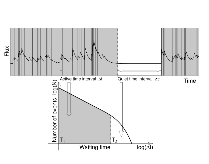
Waiting times, also called elapsed times, inter-occurrence times, inter-burst times, or laminar times, are defined by the time interval between two subsequent events, i.e., , measured from a time series of events. Simple examples are: (i) periodic processes (where the waiting time is constant and is equal to the time period); (ii) random, Poissonian, or Markov point processes (where the distribution of waiting times follows an exponential function); (iii) exponentially growing avalanche processes (where the waiting time distribution matches a scale-free power law-like function, as it is common in self-organized criticality (SOC) processes), (iv) magneto-hydrodynamic (MHD) turbulence processes (where power spectra can be represented by piece-wise power law functions of waiting time distributions, or (v) sympathetic flaring, which is an effect that is not consistent with independent flaring events (Wheatland et al. 1998). Hence, the study of waiting time distributions, applied to solar flares here, can be a powerful tool to identify and disentangle the relevant physical processes, in particular in connection with physical scaling laws (Aschwanden 2020).
In solar physics, the waiting distribution functions of solar flares has been found to be dominantly power law-like (Boffeta et al. 1999; Lepreti et al. 2001; Grigolini et al. 2002; Wheatland 2000a, 2003; Aschwanden and McTiernan 2010), unless the sample of waiting times covers a too small range or is incompletely sampled otherwise, due to selection effects (e.g., in Pearce et al. 1993; Crosby 1996), as demonstrated in comparison with larger and more complete data sets (Aschwanden and McTiernan 2010). The observationally established result of power law functions in the waiting time distribution of solar flares rules out a stationary Poisson process and requires an alternative explanation in terms of non-stationary Poisson processes (Wheatland 2000a; 2003), self-organized criticality (SOC) models (Aschwanden and McTiernan 2010; Aschwanden and Freeland 2012; Aschwanden et al. 2014), or MHD turbulence (Boffetta et al. 1999; Lepreti et al. 2001; Grigolini et al. 2002). It was argued that SOC avalanches occur statistically independently (Bak et al. 1987, 1988), and thus would predict an exponential waiting time distribution (Boffetta et al. 1999). However, inclusion of a driver with time-dependent variations, such as the solar cycle variability (Aschwanden 2011b), leads to a non-stationary Poisson process with power law behavior (Wheatland 2000a, 2003). In this Paper we study the time variability of the power law slope of waiting times in more detail and find a strong correlation between the level of solar activity in terms of the sunspot number SN(t), the annual flaring rate , and the power law slope of the waiting time distribution, which can be explained by their common magnetic drivers. Obviously, the variability of solar activity represents the most dominant physical process that modulates the value of the power law slope in solar flare waiting time distributions, an argument that has not received much attention (except in Wheatland and Litvinenko 2002; Wheatland 2003), but it puts previous modeling of waiting time distributions into a new light.
New results emerge also from the variability of the solar wind, especially from the renewed interest in switchback events, as observed by the Parker Solar Probe (PSP) mission. Switchbacks are sudden deflections of the magnetic field that have been found to be ubiquitous in the inner heliosphere. These events are likely to play an important role in structuring the young solar wind (Mozer et al. 2002; Tenerani et al. 2020; Horbury et al. 2020; Dudok de Wit et al. 2020). Their origin, however, remains elusive.
The structure of the paper entails observations and data analysis in Section 2, discussions in Section 3, and conclusions in Section 4.
2 Observations and Data Analysis
2.1 Previous Studies of Solar Flare Hard X-rays
In Table 1 we compile power law slopes of published waiting time distributions of solar flares, which we briefly describe in turn.
The study of Pearce et al. (1993) determines a total of 8319 waiting times (within a time range of min during the observation period of 1980-1985), using data from the Hard X-ray Burst Spectrometer (HXRBS) onboard the Solar Maximum Mission (SMM). Similarly, Biesecker (1994) detects a total of 6596 waiting times, using Burst And Transient Source Experiment (BATSE) onboard the Compton Gamma Ray Observatory (CGRO). A much smaller data set with 182 waiting times was obtained from the Wide Angle Telescope for Cosmic Hard X-rays (WATCH) onboard the GRANAT satellite (Crosby 1996). More extended statistics in hard X-ray wavelengths was gathered from the International Cometary Explorer (ICE) onboard the International Sun/Earth Explorer (ISEE-3) (Wheatland et al. 1998), HXRBS/SMM (Aschwanden and McTiernan 2010), BATSE/CGRO (Grigolini et al. 2002; Aschwanden and McTiernan 2010), and the Ramaty High Energy Solar Spectroscopic Imager (RHESSI) (Aschwanden and McTiernan 2010).
These studies are all based on hard X-ray solar flare catalogs, where waiting times are found within a range of hrs (see time ranges in Table 1), detected above a typical flux threshold of cts s-1 at hard X-ray energies of keV. Most waiting time distributions are self-similar (or scale-free) and consequently exhibit a power law scaling. We find only two exceptions, one is an exponential case, and another is a double-exponential case, see column 5 in Table 1. Thus, most of the waiting time distributions of hard X-ray data can be fitted with a power law function, with a typical slope of (see column 6 in Table 1), except for two cases with relatively small waiting time ranges. These two cases exhibit unusual low values of (Pearce et al. 1993; Crobsy 1996), because the fitted range is too narrow and suffers from incomplete sampling (Aschwanden and McTiernan 2010). Hence we discard these two dubious cases in the following analysis.
2.2 Previous Studies of Solar Flare Soft X-rays
More waiting time distributions of solar flares were sampled in soft X-ray wavelengths, making use of the 1-8 Å flux data observed with the Geostationary Orbiting Earth Satellite (GOES), which yields an uninterrupted time series of up to 47 years (from 1974 to present). Subsets of GOES time series in different year ranges were analyzed by Boffetta et al. (1999), Wheatland (2000a, 2003), and Lepreti et al. (2001). These data are ideal for waiting time statistics, since the duty cycle of GOES data is very high (94%) thanks to the geostationary orbit. The number of solar flares above a threshold of the C-class level ( W m-2) amounts to 35,221 events, while a deep survey with automated flare detection and with times higher sensitivity revealed a total of 338,661 events (Aschwanden and Freeland 2012). This data set provides the largest statistics of waiting times and is investigated in Section 2.5. All waiting time distributions could be fitted with a “thresholded” power law distribution (Aschwanden 2015), also called Pareto function (Eq. 6), or Lomax function (Lomax 1954; Hosking and Wallis 1987), which yields here power law slopes in the range of (see column 6 in Table 1). Note that these results encompass a large range of power law slopes that needs to be explained by any theoretical model. Moreover, the formal errors or uncertatinties in the power law slopes is typically , which is much smaller than the spread of the slope values , and thus cannot be explained with a single theoretical constant.
2.3 Previous Studies of Coronal Mass Ejections
There is a general consensus now that solar flare events and coronal mass ejections (CMEs) have very high mutual association rates, especially for eruptive flare events, so that the event statistics of one event group can be used as a proxy of the other event group. Hence we expect that the waiting time distributions of solar flares and CMEs are similar. Wheatland (2003) sampled the waiting time distributions of CMEs based on Large Angle Solar Spectrometric Coronagraph (LASCO) data from the Solar and Heliospheric Observatory (SOHO) spacecraft. These waiting time distributions could be fitted with thresholded power law (or Pareto) functions also, with power law slopes in the range of , sampled in different time phases of the solar cycle (see column 6 in Table 1). It turns out that the flare waiting times produce similar power law slopes as the CME waiting times, if one compares data from the same phase of the solar cycle.
2.4 Solar Cycle Dependence of Waiting Times
Wheatland (2003) examined the distribution of waiting times between subsequent CMEs in the LASCO CME catalog for the years 1996-2001 and found a power-law slope of for large waiting times (at 10 hours). Wheatland (2003) noted that the power law index of the waiting-time distribution varies with the solar cycle: for the years 1996-1998 (a period of low activity), the power-law slope is , and for the years 1999-2001 (a period of higher activity), the slope is . Wheatland (2003) concluded that the observed CME waiting time distribution, and its variation with the solar cycle, may be understood in terms of CMEs occurring as a time-dependent Poisson process. The same can be said for solar flares, since flares and CMEs are highly correlated.
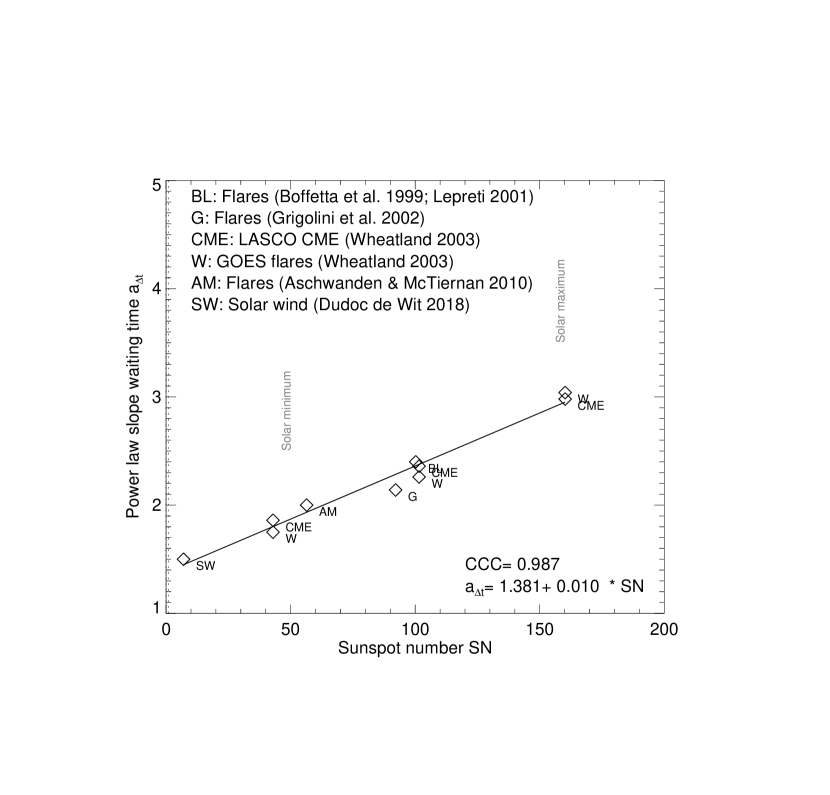
In order to prove this hypothesis, we investigate the functional relationship between the waiting time power law slope and the level of solar activity, which we quantify by the sunspot number SN. We list the mean annual sunspot number (from the Royal Observatory in Belgium, www.sidc.be/silso/) in Table 2 for the years of 1974-2012. Then we average the annual sunspot numbers over the range of years that correspond to each data set given in Table 1: 1980-1989 (HXRBS/SMM; Aschwanden and McTiernan 2010); 1991-1993 (BATSE/CGRO; Aschwanden and McTiernan 2010); 1991-2000 (BATSE/CGRO; Grigolini et al. 2002); 2002-2008 (RHESSI; Aschwanden and McTiernan 2010); 1975-1999 (GOES; Boffetta et al. 1999; Wheatland 2000a; Lepreti et al. 2001), 1996-2001 (GOES, LASCO/SOHO; Wheatland 2003); 1996-1998 (GOES, LASCO/SOHO; Wheatland 2003); 1999-2001 (GOES, LASCO/SOHO; Wheatland 2003); 2018 (PSP; Dudok de Wit et al. 2020). Then we plot the power law slopes as a function of the annually averaged sunspot numbers SN in Fig. 1 and find a linear relationship of
| (1) |
as confirmed by the high value of the Pearson’s cross-correlation coefficient (CCC=0.987). The sunspot number varies from SN40 during the solar cycle minimum to SN160 during the solar cycle maximum. Interestingly, this result is robust in the sense that it predicts the same linear relationship even when different event detection thresholds, different phenomena (flares, CMEs, solar wind switchbacks), and different wavelengths (hard X-rays, soft X-rays) are used. This empirical linear relationship explains a variety of observed power law slopes for waiting times, covering a range of (Fig. 1).
2.5 Annual GOES Waiting Time Statistics
The published power law slopes mentioned in the previous Section mostly cover multi-year ranges. In the following task we examine the degree of correlation between the annual power law slopes of waiting times and the annual sunspot numbers from the entire 47-year data set of GOES flares. We break the data sets down into 39 annual groups (from 1974 to 2012), for the same time epoch as we performed automated flare detection in a previous study (Aschwanden and Freeland 2012). For each of the 39 data sets we fit a thresholded power law (or Pareto-type) distribution) (Eq. 6), parameterized with .
The published power law slopes are usually fitted in the inertial range and have a mean value that corresponds to the (logarithmic) midpoint of the waiting time distribution. In contrast, the fitting of a power law function plus an exponential cutoff has a bias to yield steeper power law slopes at the upper end , where the slope is steepest. In order to make the two methods compatible, we can define an empirical correction factor , for which we find an average value of ,
| (2) |
Applying this correction to the upper limits (crosses in Fig. 3a), the corrected power law slopes (crosses in Fig. 3b) become fully compatible with the published power law values (diamonds in Figs. 1, 3a, and 3b) based on standard power law fitting methods in the observed inertial ranges.
We present the fits of the Pareto distribution functions (Eq. 6) in Fig. 2 and list the years, the number of events , the power law slope of the waiting times, the goodness-of-fit , the lower and upper bounds of the fitted range, the decades of the inertial range , and the annual sunspot number SN in Table 2.
Plotting the time evolution of the power law slope in annual steps (Fig. 4a), we see a solar cycle variation that is similar to the time variation of the annual sunspot number SN(t) (Fig. 4b), or the flaring rate per year (Fig. 4c). Fitting a linear regression between the two parameters, we find a linear relationship of (Fig. 5a), with a correlation coefficient of CCC=0.961. This correlation corroborates the result of a linear relationship between the power law slope and the sunspot number from previous work (Fig. 1).
The value of the power law slope , after the inertial range correction, appears not to depend on event detection thresholds, efficiency of event detection, and pulse pile-up effects. For long-duration flare events, short flares could pile-up upon on long tails, violating the separation of time scales, and possibly steepening the power law slope of waiting times. Our automated flare detection is about 10 times more sensitive than the standard NOAA flare catalog, while the GOES C-class level is often used as a threshold in statistical studies.
2.6 Switchback Events detected with the Parker Solar Probe
More recently, the Parker Solar Probe (PSP) (Fox et al. 2015) has revealed the omnipresence of so-called switchback events in Alfvénic solar wind streams within a distance of 50 solar radii from the Sun. These events show up as sudden deflections of the (otherwise mostly radial) magnetic field of the young solar wind. Because switchbacks can easily be identified as discrete events, they offer yet another opportunity for investigating how waiting time distributions are influenced by solar activity.
Dudok de Wit et al. (2020) analyzed a time interval that is centered on the first perihelion pass of November 6, 2018 and runs from November 1st to November 10, 2018. The vector magnetic field onboard PSP is measured by the MAG magnetometer from the FIELDS instrument suite (Bale et al. 2016). The waiting time and residence time scales of switchbacks occur predominantly in the inertial range of the solar wind: the sampled waiting time distribution covers a range of hours. The power law slope varies in a range of (Dudok de Wit et al. 2020).
Here we revisit these results by considering a new data set of =19,543 individual switchback events that have been automatically selected by feature recognition using magnetic field data sampled at 0.1 s. Switchback events are defined here as a step function in the deflection of the magnetic field with respect to the orientation of the Parker spiral. These events are required to be aligned for some duration before and after the event. Waiting times with s are believed to be biased by smaller events, and waiting times with s are increasingly polluted by ion cyclotron waves and are discarded anyway. Let us stress that unlike with flare events, in which large flares can be followed by smaller ones, no switchbacks can occur during long switchback events. For that reason the long tails of the distributions may differ, because the separation of time scales (waiting times, flare durations) is violated.
We show the waiting time distribution in Fig. (6), fitted with two theoretical models (see Section 3.1), with (i) the Pareto distribution that is close to a power law function at large waiting times (Fig. 6a), and (ii) with a Pareto plus an exponential cutoff (Fig. 6b). The latter model yields a superior fit (Fig. 6b), with a power law slope of and a goodness-of-fit , which indicates that a power law with an exponential cutoff is a more realistic description of the waiting time distribution.
3 Discussion
3.1 Pareto-Type Waiting Time Distribution Function
The statistics of waiting times bears information that enables us to discriminate between two statistical distribution functions: (i) random processes with Poissonian noise, and (ii) clustering of events within individual intervals (such as Omori’s law for earthquakes, which exhibits precursors and aftershock events during a major complex earthquake event). A Poissonian process in the time domain is a sequence of randomly distributed and thus statistically independent events, producing a waiting time distribution of time intervals that follows an exponential function,
| (3) |
where is the mean flaring rate or mean reciprocal waiting time, and is the probability density function (or differential occurrence frequency). Therefore, if individual events are produced by a physical random process, the occurrence frequency of waiting times should follow such an exponential-like function (Eq. 3).
In reality, however, almost all observed waiting time distributions of solar flare events exhibit a power law-like distribution for the probability function , rather than an exponential function. In an attempt to match this observational constraint, a non-stationary flare occurrence rate was defined that varies as a function of time in piece-wise time intervals or Bayesian blocks (Wheatland et al. 1998; Wheatland 2000a, 2001, 2003). Some examples of such non-stationary Poisson processes are given in Aschwanden and McTiernan (2010) and Aschwanden (2011a, Section 5.2). For instance, it includes an exponentially growing (or decaying) flare rate that produces a Pareto-type distribution for the waiting time distribution with a power law slope of 3,
| (4) |
It includes also a flare rate that varies highly intermittently in form of -functions, which produces a Pareto distribution also, but with a different power law slope of 2,
| (5) |
In order to generalize these two solutions (Eqs. 4 and 5) into a single function, we can define a Pareto-type distribution with a variable power law slope , as parameterized in Eqs. (1) and (2),
| (6) |
A more general expression of the waiting time distribution that includes finite system size effects, in terms of an exponential-like cutoff near the longest waiting time intervals ,
| (7) |
which yields a superior fit, as shown in the case of solar wind switchbacks (Fig. 6b). This equation fully describes the observed waiting time distributions (as shown in Figs. 2 and 6), expressed by five parameters (, SN). The mean waiting time , approximately represents the lower bound of the inertial range and separates the range of incompletely sampled events (see Fig. 6b) from the scale-free power law range of completely sampled events. The waiting time demarcates the e-folding cutoff due to finite system size effects. is an offset that depends on the instrumental sensitivity, the flux threshold in the automated detection of waiting times, and pulse-pileup effects. For long-duration flare events, short flares may break up long waiting times into smaller waiting times, which steepens the power law slope. Since the sunspot number SN is an observable that is known from earlier centuries up to today (Table 2), there are only four free variables left (), which can be derived empirically by fitting Eqs. (7) to an observed data set. Note that the maximum power law slope relates to the mean power law slope by a correction factor given in Eq. (2).
The fact that most waiting time distributions exhibit a power law-like function, rather than an exponential-like function, clearly requires a non-stationary Poisson process (Wheatland et al;. 1998; Wheatland 2000a, 2001), which implies that the flaring rate has a substantial time variability. The time variability of the mean flaring rate has been found to be highly correlated with the annual sunspot number (Fig. 4), and thus is modulated by Hale’s magnetic cycle of solar activity. Apparently, the mean waiting time between solar flares depends on the global magnetic flux (quantified by the sunspot number), but not on the flare size (or peak count rate) according to observations, in contrast to theoretical expectations of energy storage models (Rosner and Vaiana 1978; Wheatland 2000b).
3.2 Flare Model of Waiting Times
All fitted waiting time distributions shown in Fig. 2 are modulated by annual variations of the solar cycle. On shorter (than annual) time scales, the flaring rate varies also, as statistics based on Bayesian-block decomposition reveal (Wheatland et al. 1998; Wheatland 2000b, 2001, 2003; Wheatland and Litvinenko 2002). A flare model that possibly could explain the waiting time distribution function was proposed (Wheatland and Litvinenko 2002; Wheatland and Craig 2006), based on the assumptions of: (i) Alfvénic time scale for crossing the magnetic reconnection region, (ii) 2-D geometry of reconnetion region (or separatrix); and (iii) correlation of flare energy build-up (or storage) and flare waiting time. This model, however, is not consistent with observations, which show no correlation between flare sizes and flare waiting times (Crosby 1996; Wheatland 2000b; Georgoulis et al. 2001), not even between subsequent flares of the same active region (Crosby 1996; Wheatland 2000b). Consequently, such theoretical flare energy storage models (Rosner and Vaiana 1978; Lu 1995) have been abandoned. A more likely model involves interchange reconnection between coronal loops and open magnetic fields (Zank et al. 2020).
3.3 Self-Organized Criticality Models
The fractal-diffusive avalanche model of a slowly-driven self-organized criticality (FD-SOC) system (Aschwanden 2012, 2014; Aschwanden and Freeland 2012; Aschwanden et al. 2016), expanded from the original version of Bak et al. (1987, 1988), is based on a scale-free (power law) size distribution function of avalanche (or flare) length scales ,
| (8) |
with the Euclidean spatial dimension (which can have values of d=1, 2, or 3). This reciprocal relationship between the spatial size of a switchback structure and the occurrence frequency is visualized in Fig. 8, for the case of a space-filling avalanche mechanism, but it holds for rare events in terms of relative probabilities also.
The transport process of an avalanche is described by classical diffusion according to the FD-SOC model, which obeys the scaling law,
| (9) |
with for classical diffusion. Substituting the length scale with the duration of an avalanche event, using Eq. (8-9) and the derivative , predicts a power law distribution function for the size distribution of time durations ,
| (10) |
for and , defining the waiting time power law slope ,
| (11) |
We can now estimate the size distribution of waiting times by assuming that the avalanche durations represent upper limits to the waiting times during flaring time intervals, while the waiting times become much larger during quiescent time periods. Such a bimodal size distribution with a power law slope of at short waiting times (), and an exponential-like cutoff function at long waiting times , is depicted in Fig. 7,
| (12) |
Thus, this FD-SOC model predicts a power law with a slope of in the inertial range, and a steepening cutoff function at longer waiting times. Observationally, we find a range of , varying as a function of the solar activity, but the solar cycle modulation is not quantified in any SOC model (Aschwanden 2019b).
3.4 MHD Turbulence Processes
Boffetta et al. (1999) argue that the statistics of solar flare (laminar or quiescent) waiting times indicate a physical process with complex dynamics with long correlation times, such as in chaotic models, in contradiction to stationary SOC models that predict Poisson-like statistics. They consider chaotic models that include the destabilization of the laminar phases and subsequent restabilization due to nonlinear dynamics, as invoked in their shell model of MHD turbulence.
Similarly, Lepreti et al. (2001) attribute the origin of the observed waiting time distribution to the fact that the physical process underlying solar flares is statistically self-similar in time and is characterized by a certain amount of “memory”. They find that the power law distribution can be modeled by a Lévy function which can explain a power law exponent of (Eq. 4) in the waiting time distribution.
Grigolini et al. (2002) develop a technique called diffusion entropy method to reproduce the observed waiting time distribution function, which evaluates the entropy of the diffusion process generated by the time series. Note that classical diffusion (Eq. 9) has been employed in SOC models (Aschwanden 2012), which may be related to the diffusion entropy method, since both models produce a similar scaling of short waiting times, with power law slopes in the range of (Table 1). The change of the power law index from to has been interpreted in terms of a phase transition from the Gaussian to the Lévy basin of attraction (Grigolini et al. 2002).
3.5 Switchback events observed with Parker Solar Probe
The novel phenomenon of the so-called switchback events were sampled in situ with the PSP in the solar wind at a distance of AU. Switchback events have durations of less than 1 s to more than an hour. Hallmarks of switchback events are reversals in the radial field component (with respect to the Parker spiral geometry), which can produce deflection angles from a few degrees to nearly in the fully anti-sunward direction (Dudok de Wit et al. 2020). A switchback event can be quantified either by the magnetic potential energy,
| (13) |
or by the normalized deflection angle ,,
| (14) |
Moreover, we can sample the waiting times of subsequent events, which resulted into a power law-like inertial range of s, an exponential cutoff at s, and an undersampled range at s (Fig. 6b). The power law slope of the waiting time distribution, (Fig. 6), is measured in the year 2018, close to the minimum of the solar cycle, and follows the same trend as solar flares and CMEs (Fig. 1).
This close similarity of the slopes obtained with solar flares and with switchbacks is intriguing and could be the signature of common drivers. However, as of today the origin of switchbacks is unclear. They may be generated either locally in the upper solar corona or by instabilities such as plasma jets occurring much deeper in the corona. In addition, there are also several differences in the way flares and switchbacks are registered: the flaring rate, for example, includes independent and sympathetic flares occurring everywhere on the solar disc and at the limb, while switchback events are recorded at one single point in space only, along the satellite orbit. In addition, the impact of local solar wind conditions, and the relative speed of PSP on the rate of switchback events still has to be properly investigated. Therefore, while the similarity of the waiting time distributions is likely to be deeply rooted in the underlying physical processes, it is premature to conclude about the connection between the two types of events.
Long-term memories, expressed by the residence time of switchback events are then expected to scale with the flare or CME duration , which is predicted from SOC models to follow a power law distribution function of (Eq. 10), and a proportional distribution of for short waiting times (Eq. 12). Both the waiting time and the residence time distribution of these switchback deflections tend to follow a power law and are remarkably similar (Dudok de Wit et al. 2020). The long memory we observe is most likely associated with the strong spatial connection between adjacent magnetic flux tubes and their common photospheric footpoints (Dudok de Wit et al. 2020). Consequently, it has been proposed that switchback events are modulated by impulsive flare (or CME) events in the lower corona (Roberts et al. 2018; Tenerani et al. 2020; Zank et al. 2020).
4 Conclusions
In this study we investigate the statistics of waiting time distributions of solar flares, CMEs, and solar wind switchback events. The motivation for this type of analysis method is the diagnostics of stationary and non-stationary Poissonian random processes, SOC systems, and MHD turbulence systems. The observational analysis is very simple, since only an event catalog with the starting times of the events is necessary to sample waiting times . We obtain the following results:
-
1.
Using the statistics of hard X-ray solar flares (using flare catalogs from HXRBS/SMM, BATSE/CGRO, WATCH, ICE/ISEE-3, RHESSI) we find power law distribution functions with slopes in the range of , following a linear regression fit of SN and a cross-correlation coefficient of CCC=0.987 (Fig. 1). This trend clearly indicates that the waiting time power law slope is foremost correlated with the sunspot number (or the flaring rate), which is fully consistent with previous findings (Wheatland and Litvinenko 2002; Wheatland 2003).
-
2.
Using the statistics of soft X-ray flares, sampled by GOES over 47 years in annual intervals, but with a 10 times higher sensitivity, we perform fits with a Pareto-type distribution function (Fig. 2), which consists of an inertial (power law) range, an exponential cutoff range, and a range of under-sampling. The fits clearly show power law slopes that are modulated by the four solar cycles, strongly correlated with the annual sunspot number and the annual flaring rate (Figs. 4, 5), consistent with the hard X-ray flare results.
-
3.
We sample 19,452 magnetic field switchback events from data observed with the Parker Solar Probe and find a power law slope of . A theoretical value of is predicted for short waiting times ( s) by a self-organized criticality model during contigous flaring time episodes, while an exponentially droping cutoff is expected for long waiting times ( s). Hence we propose that a realistic waiting time distribution contains a power law part for short waiting times and an exponential part for long waiting times (Eq. 12), which reflects the duality between flaring and quiescent episodes, corresponding to a combination of non-stationary and stationary Poissonian components, which can be modeled with piece-wise Bayesian time intervals (e.g., Wheatland and Litvinenko 2002).
-
4.
Although the four theoretical models discussed here (non-stationary Poissonian, stationary Poissonian, SOC, and MHD turbulence) can all explain some partial aspects of the obseved waiting time distribution functions (exponential, power law), none of them predicts the most dominating parameter, namely the time-dependent modulation of the magnetic solar cycle, which can be modeled in terms of the flaring rate or sunspot number. This result suggests that the variability observed in the solar wind is modulated by flares and CMEs originating in the lower corona, rather than in localized heliospheric sources. Further conceptual uncertainties in data modeling include under-sampling and thresholding in automated event detection, pulse pile-up of small events in the wake of larger events, Bayesian interval selection, distinction of flaring and quiescent episodes, and exponential cutoff at maximum waiting times. A Pareto-type function with an exponential cutoff appears to be the most appropriate choice to fit the observed waiting time distributions.
Waiting time statistics has been applied to many nonlinear phenomena. While we deal here with three phenomena only (solar flares, CMEs, solar wind switchback events), other analyzed data include earthquakes (Omori’s law), auroral emission, substorms in magnetosphere, solar radio bursts, stellar flares (Aschwanden 2019a; Aschwanden and Güdel 2021), black hole accretion disks (see Aschwanden 2011a, 2016, and references therein).
Acknowledgements: Part of the work was supported by NASA contract NNG04EA00C of the SDO/AIA instrument and NNG09FA40C of the IRIS instrument.
References
Aschwanden, M.J. and McTiernan, J.M. 2010, Reconciliation of waiting time statistics of solar flares observed in hard X-rays, ApJ 717, 683
Aschwanden, M.J. 2011a Self-Organized Criticality in Astrophysics. The Statistics of Nonlinear Processes in the Universe, ISBN 978-3-642-15000-5, Springer-Praxis: New York, 416p.
Aschwanden, M.J. 2011b, The state of self-organized criticality of the Sun during the last 3 solar cycles. I. Observations, SoPh 274, 99
Aschwanden, M.J. 2012, A statistical fractal-diffusive avalanche model of a slowly-driven self-organized criticality system A&A 539:A2.
Aschwanden, M.J. and Freeland, S.M. 2012, Automated solar flare statistics in soft X-rays over 37 years of GOES observations: The invariance of SOC during 3 solar cycles, ApJ 754:112.
Aschwanden, M.J. 2014, A macroscopic description of self-organized systems and astrophysical applications, ApJ 782, 54
Aschwanden, M.J. 2015, Thresholded power law size distributions of instabilities in astrophysics, ApJ 814:19.
Aschwanden, M.J. 2016, 25 Years of SOC: Solar and astrophysics SSRv 198:47.
Aschwanden, M.J. 2019a, Self-organized criticality in solar and stellar flares: Are extreme events scale-free ? ApJ 880, 105.
Aschwanden, M.J. 2019b, Nonstationary fast-diven, self-organized criticality in solar flares, ApJ 887:57
Aschwanden, M.J. 2020, Global energetics of solar flares. XII. Energy scaling laws, ApJ (in press).
Aschwanden M.J. and Güdel, M. 2021, Self-organized criticality in stellar flares, (subm.)
Bak, P., Tang, C., and Wiesenfeld, K. 1987, Self-organized criticality - An explanation of 1/f noise, Physical Review Lett. 59/27, 381-384.
Bak, P., Tang, C., and Wiesenfeld, K. 1988, Self-organized criticality, Physical Rev. A 38/1, 364-374.
Bale, S.D., Goetz, K., Wygant, J.R. et al. 2016, The FIELDS instrument suite for Solar Probe Plus, SSRv 204, 49
Biesecker, D.A. 1994 On the occurrence of solar flares observed with the burst and transient source experiment PhD Thesis, University of New Hampshire
Boffetta, G., Carbone, V., Giuliani, P., Veltri, P., and Vulpiani, A. 1999, Power Laws in Solar Flares: Self-Organized Criticality or Turbulence? Phys.Rev.Lett. 83, 4662
Crosby, N.B., Georgoulis, M., and Villmer, N. 1996, A comparison between the WATCH flare data statistical properities and predictions of the statistical flare model, in Proc. 8th SOHO Workshop (eds. J.C. Vial and B. Kaldeich-Schuermann), ESA 446, Estec Nordwijk, p.247
Dudok de Wit, P., Krasnoselskikh, V.V., Bale, S.D., et al. 2020, Switchbacks in the near-Sun magnetic field. Long memory and impact on the turbulence cascade, ApJSS 246:39
Fox, N.J., Velli, M.C., Bale, S.D., Decker, R., Driesman, A., Howard et al. 2016, The Solar Probe Plus Mission: Humanity’s First Visit to Our Star, Space Science Reviews, 204, 7.
Georgoulis, M.K., Vilmer, N., Croby, N.B. 2001,2 A Comparison Between Statistical Properties of Solar X-Ray Flares and Avalanche Predictions in Cellular Automata Statistical Flare Models, A&A 367, 326
Grigolini, P., Leddon,D., and Scafetta,N. 2002, Diffusion entropy and waiting time statistics of hard X-ray solar flares, Phys.Rev.Lett E, 65/4. id. 046203
Horbury, S., Woolley, T., Laker R., Matteini, L. et al. 2020 Sharp Alfvenic impulses in the Near-Sun solar wind, ApJSS 246:45
Hosking, J.M.R. and Wallis, J.R. 1987, Technometrics 29, 339.
Krasnoselskikh, V., Larosa, A., Agapitov, O., Dudok de Wit, T., 2020, Localized magnetic Field structures and their boundaries in the near-Sun solar wind from Parker Solar Probe measurements, ApJ 893, 93.
Lepreti, F., Carbone, V., and Veltri,P. 2001, Solar flare waiting time distribution: varying-rate Poisson or Levy function? ApJ 555, L133
Lomax, K.S. 1954, , J. Am. Stat. Assoc. 49, 847
Lu, E.T. 1995, Constraints on energy storage and release models for astrophysical transients and solar flares, ApJ 447, 416.
Mozer, F.S., Agapitov, O.V., Bale, S.D., Bonnell, J.W. et al. 2020, Switchbacks in the solar magnetic field: Their evolution, their contentk, and their effects on the plasma, ApJSS 246:68
Pearce, G., Rowe, A.K., and Yeung, J. 1993, A statistical analysis of hard X-ray solar flares. Astrophys. Space Science 208, 99.
Roberts M.A., Uritsky, V.M., DeVore, C.R., and Karpen,J.T. 2018, Simulated encounters of the Parker Solar Probe with a Coronal-hole Jet, ApJ 866, 14
Rosner, R., and Vaiana, G.S. 1978, Cosmic flare transients: constraints upon models for energy storage and release derived from the event frequency distribution, ApJ 222, 1104
Tenerani, A., Velli, M., Matteini, L., et al. 2020, Magnetic Field Kinks and Folds in the Solar Wind, ApJS 246, 32
Wheatland, M.S., Sturrock,P.A., and McTiernan,J.M. 1998, The waiting-time distribution of solar flare hard X-rays ApJ 509, 448-455.
Wheatland,M.S. 2000a, The origin of the solar flare waiting-time distribution, ApJ 536, L109.
Wheatland,M.S. 2000b, Do solar flares exhibit an internal-size relationship, SoPh 191, 381-389.
Wheatland, M.S. 2001, Rates of flaring in individual active regions, SoPh 203, 87-106.
Wheatland, M.S. and Litvinenko, Y.E. 2002, Understanding Solar Flare Waiting-Time Distributions, SoPh 211, 255-274.
Wheatland, M.S. 2003, The Coronal Mass Ejection Waiting-Time Distribution SoPh 214, 361-373.
Wheatland, M.S., and Craig, I.J.D. 2006, Including Flare Sympathy in a Model for Solar Flare Statistics, SoPh 238, 73-86.
Zank, G.P., Nakanotani, M., Zhao, L.L., Adhikari, L., and Kasper, J., 2020, The origin of switchbacks in the solar corona, ApJ 903:1
| Observations | Observations | Number | Waiting | WTD | Powerlaw | References |
| year of events | spacecraft or | range | time | |||
| instrument | ||||||
| 1980-1985 | HXRBS/SMM | 8319 | hrs | PL | Pearce et al. (1993) | |
| 1991-2000 | BATSE/CGRO | 6596 | hrs | E | Biesecker (1994) | |
| 1990-1992 | WATCH/GRANAT | 182 | hrs | PE | Crosby (1996) | |
| 1978-1986 | ICE/ISEE-3 | 6916 | hrs | DE | Wheatland et al. (1998) | |
| 1980-1989 | HXRBS/SMM | 12,772 | hrs | PL | Aschwanden & McTiernan (2010) | |
| 1991-1993 | BATSE/CGRO | 4113 | hrs | PL | Aschwanden & McTiernan (2010) | |
| 1991-2000 | BATSE/CGRO | 7212 | hrs | PL | Grigolini et al. (2002) | |
| 2002-2008 | RHESSI | 11,594 | hrs | PL | Aschwanden & McTiernan (2010) | |
| 1975-1999 | GOES 1-8 A | 32,563 | hrs | PL | Boffetta et al. (1999) | |
| 1975-1999 | GOES 1-8 A | 32,563 | hrs | PL | Wheatland (2000a), Lepreti et al. (2001) | |
| 1996-2001 | GOES 1-8 A | 4645 | hrs | PL | Wheatland (2003) | |
| 1996-1998 | GOES 1-8 A | … | hrs | PL | Wheatland (2003) | |
| 1999-2001 | GOES 1-8 A | … | hrs | PL | Wheatland (2003) | |
| 1975-2001 | GOES 1-8 A | … | hrs | PL | Wheatland and Litvinenko (2002) | |
| Solar min | GOES 1-8 A | … | hrs | PL | Wheatland and Litvinenko (2002) | |
| Solar max | GOES 1-8 A | … | hrs | PL | Wheatland and Litvinenko (2002) | |
| 1996-2001 | SOHO/LASCO | 4645 | hrs | PL | Wheatland (2003) | |
| 1996-1998 | SOHO/LASCO | … | hrs | PL | Wheatland (2003) | |
| 1999-2001 | SOHO/LASCO | … | hrs | PL | Wheatland (2003) | |
| 2018 | PSP | … | hrs | PL | Dudok de Wit et al.(2018) | |
| 2018 | PSP | … | hrs | PE | This work |
| Year | Number | power law | best-fit | lower | upper | decades | Sunspot |
|---|---|---|---|---|---|---|---|
| of events | slope | chi-square | bound | bound | number | ||
| [hrs] | [hrs] | SN | |||||
| 1974 | 158 | 1.530.12 | 0.95 | 0.078 | 19.869 | 2.4 | 49.2 |
| 1975 | 2864 | 1.320.02 | 1.24 | 0.025 | 19.514 | 2.9 | 22.5 |
| 1976 | 1829 | 1.320.03 | 1.17 | 0.029 | 113.170 | 3.6 | 18.4 |
| 1977 | 5541 | 1.720.02 | 1.30 | 0.037 | 8.309 | 2.3 | 39.3 |
| 1978 | 16896 | 2.650.02 | 1.69 | 0.024 | 1.319 | 1.7 | 131.0 |
| 1979 | 18795 | 3.170.02 | 1.51 | 0.026 | 2.180 | 1.9 | 220.1 |
| 1980 | 15341 | 3.140.03 | 2.10 | 0.026 | 9.511 | 2.6 | 218.9 |
| 1981 | 15528 | 3.160.03 | 2.72 | 0.024 | 6.005 | 2.4 | 198.9 |
| 1982 | 15963 | 2.820.02 | 1.98 | 0.023 | 4.945 | 2.3 | 162.4 |
| 1983 | 9566 | 2.490.03 | 3.27 | 0.038 | 2.819 | 1.9 | 91.0 |
| 1984 | 6891 | 1.930.02 | 2.53 | 0.035 | 8.690 | 2.4 | 60.5 |
| 1985 | 2776 | 1.650.03 | 1.53 | 0.051 | 13.588 | 2.4 | 20.6 |
| 1986 | 2337 | 1.530.03 | 2.04 | 0.046 | 14.600 | 2.5 | 14.8 |
| 1987 | 4867 | 1.710.02 | 1.04 | 0.030 | 49.343 | 3.2 | 33.9 |
| 1988 | 13028 | 2.670.02 | 3.01 | 0.028 | 1.034 | 1.6 | 123.0 |
| 1989 | 17533 | 3.630.03 | 1.77 | 0.033 | 1.078 | 1.5 | 211.1 |
| 1990 | 15281 | 3.370.03 | 2.48 | 0.032 | 1.053 | 1.5 | 191.8 |
| 1991 | 16857 | 3.130.02 | 2.04 | 0.024 | 0.847 | 1.5 | 203.3 |
| 1992 | 12487 | 2.770.02 | 2.42 | 0.033 | 2.248 | 1.8 | 133.0 |
| 1993 | 9386 | 2.210.02 | 1.43 | 0.038 | 8.785 | 2.4 | 76.1 |
| 1994 | 4844 | 1.670.02 | 1.25 | 0.039 | 3.972 | 2.0 | 44.9 |
| 1995 | 2651 | 1.590.03 | 1.82 | 0.079 | 26.021 | 2.5 | 25.1 |
| 1996 | 1287 | 1.440.04 | 1.27 | 0.066 | 23.094 | 2.5 | 11.6 |
| 1997 | 3775 | 1.880.03 | 1.71 | 0.051 | 11.941 | 2.4 | 28.9 |
| 1998 | 11170 | 2.610.02 | 1.17 | 0.040 | 2.100 | 1.7 | 88.3 |
| 1999 | 14683 | 2.670.02 | 1.02 | 0.025 | 0.827 | 1.5 | 136.3 |
| 2000 | 16160 | 3.040.02 | 2.24 | 0.025 | 4.052 | 2.2 | 173.9 |
| 2001 | 16023 | 2.920.02 | 1.39 | 0.027 | 2.201 | 1.9 | 170.4 |
| 2002 | 16174 | 3.290.03 | 0.81 | 0.031 | 7.031 | 2.4 | 163.6 |
| 2003 | 12283 | 2.600.02 | 0.99 | 0.033 | 1.129 | 1.5 | 99.3 |
| 2004 | 8956 | 2.150.02 | 1.15 | 0.038 | 3.057 | 1.9 | 65.3 |
| 2005 | 6705 | 1.890.02 | 1.16 | 0.032 | 10.065 | 2.5 | 45.8 |
| 2006 | 3100 | 1.600.03 | 1.24 | 0.045 | 11.067 | 2.4 | 24.7 |
| 2007 | 1433 | 1.540.04 | 1.20 | 0.039 | 42.179 | 3.0 | 12.6 |
| 2008 | 190 | 1.510.11 | 0.96 | 0.110 | 170.120 | 3.2 | 4.2 |
| 2009 | 531 | 1.600.07 | 1.08 | 0.063 | 74.695 | 3.1 | 4.8 |
| 2010 | 3660 | 1.790.03 | 1.05 | 0.070 | 7.715 | 2.0 | 24.9 |
| 2011 | 11270 | 2.560.02 | 1.24 | 0.042 | 2.272 | 1.7 | 80.8 |
| 2012 | 13106 | 2.440.02 | 1.35 | 0.028 | 1.875 | 1.8 | 84.5 |