Improved Cooperation by Exploiting a Common Signal

Abstract.

Can artificial agents benefit from human conventions? Human societies manage to successfully self-organize and resolve the tragedy of the commons in common-pool resources, in spite of the bleak prediction of non-cooperative game theory. On top of that, real-world problems are inherently large-scale and of low observability. One key concept that facilitates human coordination in such settings is the use of conventions. Inspired by human behavior, we investigate the learning dynamics and emergence of temporal conventions, focusing on common-pool resources. Extra emphasis was given in designing a realistic evaluation setting: (a) environment dynamics are modeled on real-world fisheries, (b) we assume decentralized learning, where agents can observe only their own history, and (c) we run large-scale simulations (up to 64 agents).

Uncoupled policies and low observability make cooperation hard to achieve; as the number of agents grow, the probability of taking a correct gradient direction decreases exponentially. By introducing an arbitrary common signal (e.g., date, time, or any periodic set of numbers) as a means to couple the learning process, we show that temporal conventions can emerge and agents reach sustainable harvesting strategies. The introduction of the signal consistently improves the social welfare (by $258\%$ on average, up to $3306\%$), the range of environmental parameters where sustainability can be achieved (by $46\%$ on average, up to $300\%$), and the convergence speed in low abundance settings (by $13\%$ on average, up to $53\%$).

1. Introduction

The question of cooperation in socio-ecological systems and sustainability in the use of common-pool resources constitutes a critical open problem. Classical non-cooperative game theory suggests that rational individuals will exhaust a common resource, rather than sustain it for the benefit of the group, resulting in the ‘the tragedy of the commons’ Hardin (1968). The tragedy of the commons arises when it is challenging and/or costly to exclude individuals from appropriating common-pool resources (CPR) of finite yield Ostrom et al. (1994). Individuals face strong incentives to appropriate, which results in overuse and even permanent depletion of the resource. Examples include the degradation of fresh water resources, the over-harvesting of timber, the depletion of grazing pastures, the destruction of fisheries, etc.

In spite of the bleak prediction of non-cooperative game theory, the tragedy of the commons is not inevitable, though conditions under which cooperation and sustainability can be achieved may be more demanding, the higher the stakes. Nevertheless, humans have been systematically shown to successfully self-organize and resolve the tragedy of the commons in CPR appropriation problems, even without the imposition of an extrinsic incentive structure Ostrom (1999). E.g., by enabling the capacity to communicate, individuals have been shown to maintain the harvest to an optimal level Ostrom et al. (1994); Casari and Plott (2003). Though, communication creates overhead, and might not always be possible Stone et al. (2010). One of the key findings of empirical field research on sustainable CPR regimes around the world is the employment of boundary rules, which prescribe who is authorized to appropriate from a resource Ostrom (1999). Such boundary rules can be of temporal nature, prescribing the temporal order in which people harvest from a common-pool resource (e.g., ‘protocol of play’ Budescu et al. (1997)). The aforementioned rules can be enforced by an authority, or emerge in a self-organized manner (e.g., by utilizing environmental signals such as the time, date, season, etc.) in the form of a social convention.

Many real-world CPR problems are inherently large-scale and partially observable, which further increases the challenge of sustainability. In this work we deal with the most information-restrictive setting: each participant is modeled as an individual agent with its own policy conditioned only on local information, specifically his own history of action/reward pairs (fully decentralized method). Global observations, including the resource stock, the number of participants, and the joint observations and actions, are hidden – as is the case in many real-world applications, like commercial fisheries. Under such a setting, it is impossible to avoid positive probability mass on undesirable actions (i.e., simultaneous appropriation), since there is no correlation between the agents’ policies. This leads to either low social welfare, because the agents are being conservative, or, even worse, the depletion of the resource. Depletion becomes more likely as the problem size grows due to the non-stationarity of the environment and the global exploration problem.

We propose a simple technique: allow agents to observe an arbitrary, common signal from the environment. Observing a common signal mitigates the aforementioned problems because it allows for coupling between the learned policies, increasing the joint policy space. Agents, for example, can now learn to harvest in turns, and with varying efforts per signal value, or allow for fallow periods. The benefit is twofold: the agents learn to not only avoid depletion, but also to maintain a healthy stock which allows for large harvest and, thus, higher social welfare. It is important to stress that we do not assume any a priori relation between the signal space and the problem at hand. Moreover, we require no communication, no extrinsic incentive mechanism, and we do not change the underlying architecture, or learning algorithm. We simply utilize a means – common environmental signals that are amply available to the agents Hart and Mas-Colell (2000) – to accommodate correlation between policies. This in turn enables the emergence of ordering conventions of temporal nature (henceforth referred to as temporal conventions) and sustainable harvesting strategies.

1.1. Our Contributions

(1) We are the first to introduce a realistic common-pool resource appropriation game for multi-agent coordination, based on bio-economic models of commercial fisheries, and provide theoretical analysis on the dynamics of the environment.

(2) We propose a simple and novel technique: allow agents to observe an arbitrary periodic environmental signal. Such signals are amply available in the environment (e.g., time, date etc.) and can foster cooperation among agents.

(3) We provide a thorough (quantitative & qualitative) analysis on the learned policies and demonstrate significant improvements on sustainability, social welfare, and convergence speed.

1.2. Discussion & Related Work

As autonomous agents proliferate, they will be called upon to interact in ever more complex environments. This will bring forth the need for techniques that enable the emergence of sustainable cooperation. Despite the growing interest in and success of multi-agent deep reinforcement learning (MADRL), scaling to environments with a large number of learning agents continues to be a problem Ganapathi Subramanian et al. (2020). A multi-agent setting is inherently susceptible to many pitfalls: non-stationarity (moving-target problem), curse of dimensionality, credit assignment, global exploration, relative overgeneralization Hernandez-Leal et al. (2019); Matignon et al. (2012); Wiegand and Jong (2004). Recent advances in the field of MADRL deal with only a limited number of agents. It is shown that as the number of agents increase, the probability of taking a correct gradient direction decreases exponentially Hernandez-Leal et al. (2019), thus the proposed methods cannot be easily generalized to complex scenarios with many agents.

Our approach aims to mitigate the aforementioned problems of MADRL by introducing coupling between the learned policies. It is important to note that the proposed approach does not change the underlying architecture of the network (the capacity of the network stays the same), nor the learning algorithm or the reward structure. We simply augment the input space by allowing the observation of an arbitrary common signal. The signal has no a priori relation to the problem, i.e., we do not need to design an additional feature; in fact we use a periodic sequence of arbitrary integers. It is still possible for the original network (without the signal) to learn a sustainable strategy. Nevertheless, we show that the simple act of augmenting the input space drastically increases the social welfare, speed of convergence, and the range of environmental parameters in which sustainability can be achieved. Most importantly, the proposed approach requires no communication, creates no additional overhead, it is simple to implement, and scalable.

The proposed technique was inspired by temporal conventions in resource allocation games of non-cooperative game theory. The closest analogue is the courtesy convention of Danassis and Faltings (2019), where rational agents learn to coordinate their actions to access a set of indivisible resources by observing a signal from the environment. Closely related is the concept of the correlated equilibrium (CE) Aumann (1974); Nisan et al. (2007), which, from a practical perspective, constitutes perhaps the most relevant non-cooperative solution concept Hart and Mas-Colell (2000). Most importantly, it is possible to achieve a correlated equilibrium without a central authority, simply by utilizing meaningless environmental signals Danassis and Faltings (2019); Cigler and Faltings (2013); Borowski et al. (2014). Such common environmental signals are amply available to the agents Hart and Mas-Colell (2000). The aforementioned line of research studies pre-determined strategies of rational agents. Instead, we study the emergent behaviors of a group of independent learning agents aiming to maximize the long term discounted reward.

A second source of inspiration is behavioral conventions; one of the key concepts that facilitates human coordination. A convention is defined as a customary, expected, and self-enforcing behavioral pattern Young (1996); Lewis (2008). It can be considered as a behavioral rule, designed and agreed upon ahead of time Shoham and Tennenholtz (1995); Walker and Wooldridge (1995), or it may emerge from within the system itself Mihaylov et al. (2014); Walker and Wooldridge (1995). The examined temporal convention in this work falls on the latter category.

Moving on to the application domain, there has been great interest recently in CPR problems (and more generally, social dilemmas Kollock (1998)) as an application domain for MADRL Perolat et al. (2017); Leibo et al. (2017); Peysakhovich and Lerer (2018a); Hughes et al. (2018); Peysakhovich and Lerer (2018b); Jaques et al. (2019); Wang et al. (2019); Lupu and Precup (2020); Koster et al. (2020). CPR problems offer complex environment dynamics and relate to real-world socio-ecological systems. There are a few distinct differences between the CPR models presented in the aforementioned works and the model introduced in this paper: First and foremost, we designed our model to resemble reality as closely as possible using bio-economic models of commercial fisheries Clark (2006); Diekert (2012), resulting in complex environment dynamics. Second, we have a continuous action space which further complicates the learning process. Finally, we opted not to learn from visual input (raw pixels). The problem of direct policy approximation from visual input does not add complexity to the social dilemma itself; it only adds complexity in the feature extraction of the state. It requires large networks because of the additional complexity of extracting features from pixels, while only a small part of what is learned is the actual policy Cuccu et al. (2019). Most importantly, it makes harder to study the policy in isolation, as we do in this work. Moreover, from a practical perspective, learning from a visual input would be meaningless, given that we are dealing with a low observability scenario where the resource stock and the number and actions of the participants are hidden.

In terms of the methodology for dealing with the tragedy of the commons, the majority of the aforementioned literature falls broadly into two categories: Reward shaping Hughes et al. (2018); Jaques et al. (2019); Peysakhovich and Lerer (2018b), which refers to adding a term to the extrinsic reward an agent receives from the environment, and opponent shaping Koster et al. (2020); Lupu and Precup (2020); Perolat et al. (2017), which refers to manipulating the opponent (by e.g., sharing rewards, punishments, or adapting your own actions). Contrary to that, we only allow agents to observe an existing environmental signal. We do not modify the intrinsic or extrinsic rewards, design new features, or require a communication network. Finally, boundary rules emerged in Perolat et al. (2017) as well in the form of spatial territories. Such territories can increase inequality, while we maintain high levels of fairness.

2. Agent & Environment Models

2.1. Multi-Agent Reinforcement Learning

We consider a decentralized multi-agent reinforcement learning scenario in a partially observable general-sum Markov game Shapley (1953). At each time-step, agents take actions based on a partial observation of the state space, and receive an individual reward. Each agent learns a policy independently. More formally, let $\mathcal{N}=\{1,\dots,N\}$ denote the set of agents, and $\mathcal{M}$ be an $N$-player, partially observable Markov game defined on a set of states $\mathcal{S}$. An observation function $\mathcal{O}^{n}:\mathcal{S}\rightarrow\mathds{R}^{d}$ specifies agent $n$’s $d$-dimensional view of the state space. Let $\mathcal{A}^{n}$ denote the set of actions for agent $n\in\mathcal{N}$, and $\bm{a}=\times_{\forall n\in\mathcal{N}}a^{n}$, where $a^{n}\in\mathcal{A}^{n}$, the joint action. The states change according to a transition function $\mathcal{T}:\mathcal{S}\times\mathcal{A}^{1}\times\dots\times\mathcal{A}^{N}\rightarrow\Delta(\mathcal{S})$, where $\Delta(\mathcal{S})$ denotes the set of discrete probability distributions over $\mathcal{S}$. Every agent $n$ receives an individual reward based on the current state $\sigma_{t}\in\mathcal{S}$ and joint action $\bm{a}_{t}$. The latter is given by the reward function $r^{n}:\mathcal{S}\times\mathcal{A}^{1}\times\dots\times\mathcal{A}^{N}\rightarrow\mathds{R}$. Finally, each agent learns a policy $\pi^{n}:\mathcal{O}^{n}\rightarrow\Delta(\mathcal{A}^{n})$ independently through their own experience of the environment (observations and rewards). Let $\bm{\pi}=\times_{\forall n\in\mathcal{N}}\pi^{n}$ denote the joint policy. The goal for each agent is to maximize the long term discounted payoff, as given by $V^{n}_{\bm{\pi}}(\sigma_{0})=\mathds{E}\left[\sum_{t=0}^{\infty}\gamma^{t}r^{n}(\sigma_{t},\bm{a}_{t})|\bm{a}_{t}\sim\bm{\pi}_{t},\sigma_{t+1}\sim\mathcal{T}(\sigma_{t},\bm{a}_{t})\right]$, where $\gamma$ is the discount factor and $\sigma_{0}$ is the initial state.

2.2. The Common Fishery Model

In order to better understand the impact of self-interested appropriation, it would be beneficial to examine the dynamics of real-world common-pool renewable resources. To that end, we present an abstracted bio-economic model for commercial fisheries Clark (2006); Diekert (2012). The model describes the dynamics of the stock of a common-pool renewable resource, as a group of appropriators harvest over time. The harvest depends on (i) the effort exerted by the agents and (ii) the ease of harvesting a resource at that point of time, which depends on the stock level. The stock replenishes over time with a rate dependent on the current stock level.

More formally, let $\mathcal{N}$ denote the set of appropriators, $\epsilon_{n,t}\in[0,\mathcal{E}_{max}]$ the effort exerted by agent $n$ at time-step $t$, and $E_{t}=\sum_{n\in\mathcal{N}}\epsilon_{n,t}$ the total effort at time-step $t$. The total harvest is given by Eq. 1, where $s_{t}\in[0,\infty)$ denotes the stock level (i.e., amount of resources) at time-step $t$, $q(\cdot)$ denotes the catchability coefficient (Eq. 2), and $S_{eq}$ is the equilibrium stock of the resource.

$$H(E_{t},s_{t})=\begin{cases}q(s_{t})E_{t}&,\text{if }q(s_{t})E_{t}\leq s_{t}\\ s_{t}&,\text{otherwise}\\ \end{cases}$$ (1)

$$q(x)=\begin{cases}\frac{x}{2S_{eq}}&,\text{if }x\leq 2S_{eq}\\ 1&,\text{otherwise}\\ \end{cases}$$ (2)

Each environment can only sustain a finite amount of stock. If left unharvested, the stock will stabilize at $S_{eq}$. Note also that $q(\cdot)$, and therefore $H(\cdot)$, are proportional to the current stock, i.e., the higher the stock, the larger the harvest for the same total effort. The stock dynamics are governed by Eq. 3, where $F(\cdot)$ is the spawner-recruit function (Eq. 4) which governs the natural growth of the resource, and $r$ is the growth rate. To avoid highly skewed growth models and unstable environments (‘behavioral sink’ Calhoun (1962, 1973)), $r\in[-W(-1/(2e)),-W_{-1}(-1/(2e))]\approx[0.232,2.678]$, where $W_{k}(\cdot)$ is the Lambert $W$ function (see Section C for details).

$$s_{t+1}=F(s_{t}-H(E_{t},s_{t}))$$ (3)

$$F(x)=xe^{r(1-\frac{x}{S_{eq}})}$$ (4)

We assume that the individual harvest is proportional to the exerted effort (Eq. 5), and the revenue of each appropriator is given by Eq. 6, where $p_{t}$ is the price ($ per unit of resource), and $c_{t}$ is the cost ($) of harvesting (e.g., operational cost, taxes, etc.). Here lies the ‘tragedy’: the benefits from harvesting are private ($p_{t}h_{n,t}(\epsilon_{n,t},s_{t})$), but the loss is borne by all (in terms of a reduced stock, see Eq. 3).

$$h_{n,t}(\epsilon_{n,t},s_{t})=\frac{\epsilon_{n,t}}{E_{t}}H(E_{t},s_{t})$$ (5)

$$u_{n,t}(\epsilon_{n,t},s_{t})=p_{t}h_{n,t}(\epsilon_{n,t},s_{t})-c_{t}$$ (6)

2.2.1. Optimal Harvesting

The question that naturally arises is: what is the ‘optimal’ effort in order to harvest a yield that maximizes the revenue (Eq. 6). We make two assumptions: First, we assume that the entire resource is owned by a single entity (e.g., a firm or the government), which possesses complete knowledge of and control over the resource. Thus, we only have a single control variable, $E_{t}$. This does not change the underlying problem since the total harvested resources are linear in the proportion of efforts put by individual agents (Eq. 5). Second, we consider the case of zero discounting, i.e., future revenues are weighted equally with current ones. Of course firms (and individuals) do discount the future and bio-economic models should take that into account, but this complicates the analysis and it is out of the scope of this work. We argue we can still draw useful insight into the problem.

Our control problem consists of of finding a piecewise continuous control $E_{t}$, so as to maximize the total revenue ($\max_{E_{t}}\sum_{t=0}^{T}U_{t}(E_{t},s_{t})$). The maximization problem can be solved using Optimal Control Theory Ding and Lenhart (2010); Lenhart and Workman (2007). We have proven the following theorem:

The optimal control variable $E^{*}_{t}$ that solves the maximization problem $\max_{E_{t}}\sum_{t=0}^{T}U_{t}(E_{t},s_{t})$ given the model dynamics described in Section 2.2 is given by Eq. 7, where $\lambda_{t}$ are the adjoint variables of the Hamiltonians:

$$E^{*}_{t+1}=\begin{cases}E_{max},&\text{if }(p_{t+1}-\lambda_{t+1})q(F(s_{t}-H(E_{t},s_{t})))\geq 0\\ 0,&\text{if }(p_{t+1}-\lambda_{t+1})q(F(s_{t}-H(E_{t},s_{t})))<0\\ \end{cases}$$ (7)

Proof.

(sketch) We formulate the Hamiltonians Lenhart and Workman (2007); Ding and Lenhart (2010), which turn out to be linear in the control variables $E_{t+1}$ with coefficients $(p_{t+1}-\lambda_{t+1})q(F(s_{t}-H(E_{t},s_{t})))$. Thus, the optimal sequence of $E_{t+1}$ that maximizes the Hamiltonians is given according to the sign of those coefficients. See Section B for the complete proof. ∎

The optimal strategy is a bang–bang controller, which switches based on the adjoint variable values, stock level, and price. The values for $\lambda_{t}$ do not have a closed form expression (because of the discontinuity of the control), but can be found iteratively for a given set of environment parameters ($r$, $S_{eq}$) and the adjoint equations Lenhart and Workman (2007); Ding and Lenhart (2010). However, the discontinuity in the control input makes solving the adjoint equations quite cumbersome. We can utilize iterative forward/backward methods as in Ding and Lenhart (2010), but this is out of the scope of this paper.

There are a few interesting key points. First, to compute the optimal level of effort we require observability of the resource stock, which is not always a realistic assumption (in fact in this work we do not make this assumption). Second, we require complete knowledge of the strategies of the other appropriators. Third, even if both the aforementioned conditions are met, the bang-bang controller of Eq. 7 does not have a constant transition limit; the limit changes at each time time-step, determined by the adjoint variable $\lambda_{t+1}$, thus finding the switch times remains quite challenging.

2.2.2. Harvesting at Maximum Effort

To gain a deeper understanding of the dynamics of the environment, we will now consider a baseline strategy where every agent harvests with the maximum effort at every time-step, i.e., $\epsilon_{n,t}=\mathcal{E}_{max},\forall n\in\mathcal{N},\forall t$. This corresponds to the Nash Equilibrium of a stage game (myopic agents). For a constant growth rate $r$ and a given number of agents $N$, we can identify two interesting stock equilibrium points ($S_{eq}$): the ‘limit of sustainable harvesting’, and the ‘limit of immediate depletion’.

The limit of sustainable harvesting ($S^{\scriptscriptstyle N,r}_{\scriptscriptstyle LSH}$) is the stock equilibrium point where the goal of sustainable harvesting becomes trivial: for any $S_{eq}>S^{\scriptscriptstyle N,r}_{\scriptscriptstyle LSH}$, the resource will not get depleted, even if all agents harvest at maximum effort. Note that the coordination problem remains far from trivial even for $S_{eq}>S^{\scriptscriptstyle N,r}_{\scriptscriptstyle LSH}$, especially for increasing population sizes. Exerting maximum effort in environments with $S_{eq}$ close to $S^{\scriptscriptstyle N,r}_{\scriptscriptstyle LSH}$ will yield low returns because the stock remains low, resulting in a small catchability coefficient. In fact, this can be seen in Fig. 1 which depicts the social welfare (SW), i.e., sum of utilities, against increasing $S_{eq}$ values ($N\in[2,64]$, $\mathcal{E}_{max}=1$, $r=1$). Red dots denote the $S^{\scriptscriptstyle N,r}_{\scriptscriptstyle LSH}$. Thus, the challenge is not only to keep the strategy sustainable, but to keep the resource stock high, so that the returns can be high as well.

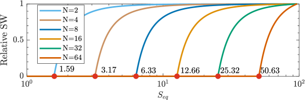
Figure 1. Social welfare (SW) – normalized by the maximum SW obtained in each setting – against increasing $S_{eq}$ values. $N\in[2,64]$, $\mathcal{E}_{max}=1$, and $r=1$. $x$-axis is in logarithmic scale.

Social welfare against increasing stock equilibrium values.

On the other end of the spectrum, the limit of immediate depletion ($S^{\scriptscriptstyle N,r}_{\scriptscriptstyle LID}$) is the stock equilibrium point where the resource is depleted in one time-step (under maximum harvest effort by all the agents). The problem does not become impossible for $S_{eq}\leq S^{\scriptscriptstyle N,r}_{\scriptscriptstyle LID}$, yet, exploration can have catastrophic effects (amplifying the problem of global exploration in MARL). The following two theorems prove the formulas for $S^{\scriptscriptstyle N,r}_{\scriptscriptstyle LSH}$ and $S^{\scriptscriptstyle N,r}_{\scriptscriptstyle LID}$.

The limit of sustainable harvesting $S^{\scriptscriptstyle N,r}_{\scriptscriptstyle LSH}$ for a continuous resource governed by the dynamics of Section 2.2, assuming that all appropriators harvest with the maximum effort $\mathcal{E}_{max}$, is:

$$S^{\scriptscriptstyle N,r}_{\scriptscriptstyle LSH}=\frac{e^{r}N\mathcal{E}_{max}}{2(e^{r}-1)}$$ (8)

Proof.

Note that for $S_{eq}>S^{\scriptscriptstyle N,r}_{\scriptscriptstyle LSH}$, $q(s_{t})E_{t}<s_{t},\forall t$, otherwise the resource would be depleted. Moreover, if $s_{0}=S_{eq}$ – which is a natural assumption, since prior to any intervention the stock will have stabilized on the fixed point – then $s_{t}<2S_{eq},\forall t$. Thus, we can re-write Eq. 1 and 2 as:

$$H(E_{t},s_{t})=\frac{s_{t}}{2S_{eq}}E_{t}=\frac{s_{t}N\mathcal{E}_{max}}{2S_{eq}}$$

Let $\alpha\triangleq\frac{N\mathcal{E}_{max}}{2S_{eq}}$, and $\beta=1-\alpha$. The state transition becomes:

$$s_{t+1}=F(s_{t}-\alpha s_{t})=\beta s_{t}e^{r(1-\frac{\beta}{S_{eq}}s_{t})}$$

We write it as a difference equation:

$$\Delta_{t}(s_{t})\triangleq s_{t+1}-s_{t}=(\beta e^{r(1-\frac{\beta}{S_{eq}}s_{t})}-1)s_{t}$$

At the limit of sustainable harvesting, as the stock diminishes to $s_{t}=\delta\rightarrow 0$, to remain sustainable it must be that $\Delta_{t}(s_{t})>0$. Thus, it must be that:

$$\underset{s_{t}\rightarrow 0^{+}}{\lim}sgn(\Delta_{t}(s_{t}))>0\overset{s_{t}\rightarrow 0^{+}>0}{\Rightarrow}\beta e^{r}-1>0\Rightarrow S_{eq}>\frac{e^{r}N\mathcal{E}_{max}}{2(e^{r}-1)}$$

∎

The limit of immediate depletion $S^{\scriptscriptstyle N,r}_{\scriptscriptstyle LID}$ for a continuous resource governed by the dynamics of Section 2.2, assuming that all appropriators harvest with the maximum effort $\mathcal{E}_{max}$, is given by:

$$S^{\scriptscriptstyle N,r}_{\scriptscriptstyle LID}=\frac{N\mathcal{E}_{max}}{2}$$ (9)

Proof.

The resource is depleted if:

$$H(E_{t},s_{t})=s_{t}\Rightarrow q(s_{t})E_{t}\geq s_{t}\Rightarrow\frac{s_{t}}{2S_{eq}}E_{t}\geq s_{t}\Rightarrow S_{eq}\leq\frac{N\mathcal{E}_{max}}{2}$$

∎

2.3. Environmental Signal

We introduce an auxiliary signal; side information from the environment (e.g., time, date etc.) that agents can potentially use in order to facilitate coordination and reach more sustainable strategies. Real-world examples include shepherds that graze on particular days of the week or fishermen that fish on particular months. In our case, the signal can be thought as a mechanism to increase the set of possible (individual and joint) policies. Such signals are amply available to the agents Hart and Mas-Colell (2000); Danassis and Faltings (2019). We do not assume any a priori relation between the signal and the problem at hand. In fact, in this paper we use a set of arbitrary integers, that repeat periodically. We use $\mathcal{G}=\{1,\dots,G\}$ to denote the set of signal values.

3. Simulation Results

3.1. Setup

3.1.1. Environment Settings

Let $p_{t}=1$, and $c_{t}=0$, $\forall t$. We set the growth rate at $r=1$, the initial population at $s_{0}=S_{eq}$, and the maximum effort at $\mathcal{E}_{max}=1$. The findings of Section 2.2.2 provide a guide on the selection of the $S_{eq}$ values. Specifically we simulated environments with $S_{eq}$ given by Eq. 10, where $K=\frac{S^{\scriptscriptstyle N,r}_{\scriptscriptstyle LSH}}{N}=\frac{e^{r}\mathcal{E}_{max}}{2(e^{r}-1)}\approx 0.79$ is a constant and $M_{s}\in\mathbb{R}^{+}$ is a multiplier that adjusts the scarcity (difficulty). $M_{s}=1$ corresponds to $S_{eq}=S^{\scriptscriptstyle N,r}_{\scriptscriptstyle LSH}$.

$$S_{eq}=M_{s}KN$$ (10)

3.1.2. Agent Architecture

Each agent uses a two-layer ($64$ neurons each) neural network for the policy approximation. The input (observation $o^{n}=\mathcal{O}^{n}(S)$) is a tuple $\langle\epsilon_{n,t-1},u_{n,t-1}(\epsilon_{n,t-1},s_{t-1}),g_{t}\rangle$ consisting of the individual effort exerted and reward obtained in the previous time-step and the current signal value. The output is a continuous action value $a_{t}=\epsilon_{n,t}\in[0,\mathcal{E}_{max}]$ specifying the current effort level. The policies are trained using the Proximal Policy Optimization (PPO) algorithm Schulman et al. (2017). PPO was chosen because it avoids large policy updates, ensuring a smoother training, and avoiding catastrophic failures. The reward received from the environment corresponds to the revenue, i.e., $r^{n}(\sigma_{t},\bm{a}_{t})=u_{n,t}(\epsilon_{n,t},s_{t})$, and the discount factor was set to $\gamma=0.99$.

3.1.3. Signal Implementation

The signal is represented as a $G$-dimensional one-hot encoded vector, where the high bit is shifted periodically. The initial value was chosen at random at the beginning of each episode to avoid bias towards particular values. Throughout this paper, the term no signal will be used interchangeably to a unit signal size $G=1$, since a signal of size $1$ in one-hot encoding is just a constant input that yields no information. We evaluated signals of varying cardinality (see Section 3.6).

3.1.4. Termination Condition

An episode terminates when either (a) the resource stock falls below a threshold $\delta=10^{-4}$, or (b) a fixed number of time-steps $T_{max}=500$ is reached. We trained our agents for a maximum of $5000$ episodes, with the possibility of early stopping if both of the following conditions are satisfied: (i) a minimum of $95\%$ of the maximum episode duration (i.e., $475$ time-steps) is reached for $200$ episodes in a row, and, (ii) the average total reward obtained by agents in each episode of the aforementioned $200$ episodes does not change by more than $5\%$. In case of early stopping, the metric values for the remainder of the episodes are extrapolated as the average of the last $200$ episodes, in order to properly average across trials.

3.1.5. Measuring The Influence of the Signal

It is important to have a quantitative measure of the influence of the introduced signal. As such, we adapted the Causal Influence of Communication (CIC) Lowe et al. (2019) metric, initially designed to measure positive listening in emergent inter-agent communication. The CIC is calculated using the mutual information between the signal and the agent’s action. Please see Section D.3 for a complete description.

3.1.6. Reproducibility, Reporting of Results, Limitations

Reproducibility is a major challenge in (MA)DRL due to different sources of stochasticity, e.g., hyper-parameters, model architecture, implementation details, etc. Henderson et al. (2018); Hernandez-Leal et al. (2019); Engstrom et al. (2020). To minimize those sources, the implementation was done using RLlib, an open-source library for MADRL Liang et al. (2017). We refer the reader to Section D for a description of the architecture and hyper-parameters.

All simulations were repeated $8$ times and the reported results are the average values of the last 10 episodes over those trials (excluding Fig. 7(b) which depicts a representative trial). (MA)DRL also lacks common practices for statistical testing Henderson et al. (2018); Hernandez-Leal et al. (2019). In this work, we opted to use the Student’s T-test Student (1908) due to it’s robustness Colas et al. (2019). Nearly all of the reported results have p-values $<0.05$.

Finally, we strongly believe that the community would benefit from reporting negative results. As such, we want to make clear that the proposed solution is not a panacea for all multi-agent coordination problems, not even for the proposed domain. For example, we failed to find sustainable policies using DDPG Lillicrap et al. (2015) – with or without the signal – for any set of environment parameters. This also comes to show the difficulty of the problem at hand. We suspect that the clipping in PPO’s policy changes plays an important role in averting catastrophic failures in high-stakes environments.

3.2. Results

We present the result from a systematic evaluation of the proposed approach on a wide variety of environmental settings ($M_{s}\in[0.2,1.2]$, i.e., ranging from way below the limit of immediate depletion, $M_{s}^{\scriptscriptstyle LID}\approx 0.63$, to above the limit of sustainable harvesting, $M_{s}^{\scriptscriptstyle LSH}=1$) and population size ($N\in[2,64]$). Due to lack of space we only present the most relevant results; see Section E for a complete report (e.g., results tables, fairness, small population sizes, etc.).

In the majority of the results, we study the influence of a signal of cardinality $G=N$ compared to no signal ($G=1$). Thus, unless stated otherwise, the term ‘with signal’ will refer to $G=N$.

3.3. Sustainability & Social Welfare

3.3.1. Sustainability

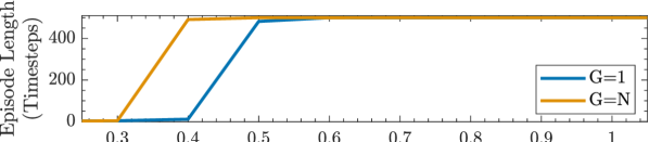
(a) $N=8$

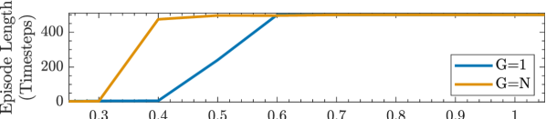
(b) $N=16$

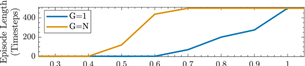
(c) $N=32$

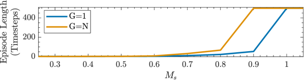
(d) $N=64$

Figure 2. Episode length, with and without the signal ($G=N$), for environments of decreasing difficulty (increasing equilibrium stock multiplier $M_{s}$).

Episode length, with and without the signal, for environments of decreasing difficulty

We declare a strategy ‘sustainable’, iff the agents reach the maximum episode duration ($500$ steps), i.e., they do not deplete the resource. Fig. 2(d) depicts the achieved episode length – with and without the presence of a signal ($G=N$) – for environments of decreasing difficulty (increasing $S_{eq}\propto M_{s}$). The introduction of the signal significantly increases the range of environments ($M_{s}$) where sustainability can be achieved. Assuming that $M_{s}\in[0,1]$ – since for $M_{s}\geq 1$ sustainability is guaranteed by definition – we have an increase of $17\%-300\%$ ($46\%$ on average) in the range of sustainable $M_{s}$ values. Moreover, as the number of agents increases ($N=32$ & $64$), depletion is avoided in non-trivial $M_{s}$ values only with the introduction of the signal. Finally, note that the $M_{s}$ value where a sustainable strategy is found increases with $N$, which demonstrates that the difficulty of the problem increases superlinearly to $N$ (given that $S_{eq}\propto M_{s}N$).

3.3.2. Social welfare

Reaching a sustainable strategy – i.e., avoiding resource depletion – is only one piece of the puzzle; an agent’s revenue depends on the harvest (Eq. 1), which in turns depends on the catchability coefficient (Eq. 2). Thus, in order to achieve a high social welfare (sum of utilities, i.e., $\sum_{n\in\mathcal{N}}r^{n}(\cdot)$), the agents need to learn policies that balance the trade-off between maintaining a high stock (which ensues a high catchability coefficient), and yielding a large harvest (which results to a higher reward). This problem becomes even more apparent as resources become more abundant (i.e., for $M_{s}=1\pm x$, i.e., close to the limit of sustainable harvesting (below or, especially, above), see Section 2.2.2). In these settings, it is easy to find a sustainable strategy; a myopic best-response strategy (harvesting at maximum effort) by all agents will not deplete the resource. Yet, it will result in low social welfare (SW).

Fig. 3 depicts the relative difference in SW, in a setting with and without the signal ($(SW_{G=N}-SW_{G=1})/SW_{G=1}$, where $SW_{G=X}$ denotes the SW achieved using a signal of cardinality $X$), for environments of decreasing difficulty (increasing $S_{eq}\propto M_{s}$) and varying population size ($N\in[8,64]$). To improve readability, changes greater than 100% are shown with numbers on the top of the bars. Given the various sources of stochasticity, we opted to omit settings in which agents were not able to reach an episode duration of more than 10 time-steps (either with or without the signal).

The presence of the signal results in a significant improvement in SW. Specifically, we have an average of $258\%$ improvement across all the depicted settings in Fig. 3, while the maximum improvement is $3306\%$. These improvements stem from (i) achieving more sustainable strategies, and (ii) improved cooperation. The former results in higher rewards due to longer episodes in settings where the strategies without the signal deplete the resource. The latter allows to avoid over-harvesting, which results in higher catchability coefficient, in settings where both strategies (with, or without the signal) are sustainable. The contribution of the signal is much more pronounced under scarcity: the difference in achieved SW decreases as $M_{s}$ increases, eventually becoming less than $10\%$ ($M_{s}>1$ for $N=8$ & $16$, and $M_{s}>1.2$ for $N=32$ & $64$). This suggests that the proposed approach is of high practical value in environments where resources are scarce (like most real-world applications), a claim that we further corroborate in Sections 3.5 and 3.7.

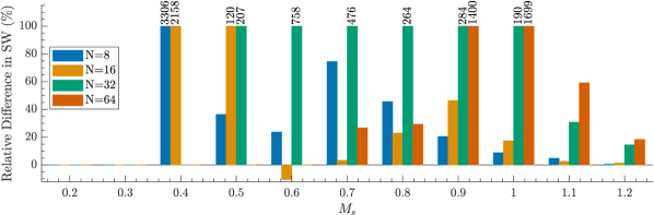
Figure 3. Relative difference in social welfare (SW) when signal of cardinality $G=N$ is introduced ($(SW_{G=N}-SW_{G=1})/SW_{G=1}$, where $SW_{G=X}$ denotes the SW achieved using a signal of cardinality $X$), for environments of decreasing difficulty (increasing $S_{eq}\propto M_{s}$) and varying population size ($N\in[4,64]$). To improve readability, changes greater than 100% are shown with numbers on the top of the bars.

Relative difference in social welfare when signal of cardinality N is introduced.

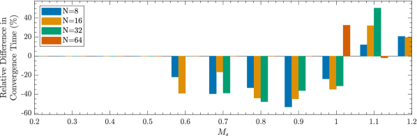
Figure 4. Relative difference in convergence time with the introduction of a signal ($(CT_{G=N}-CT_{G=1})/CT_{G=1}$, where $CT_{G=X}$ denotes the time until convergence when using a signal of cardinality $X$), for environments of decreasing difficulty (increasing $S_{eq}\propto M_{s}$) and varying population size ($N\in[8,64]$)

Relative difference in convergence time with the introduction of a signal.

3.4. Convergence Speed

The second major influence of the introduction of the proposed signal – besides the sustainability and efficiency of the learned strategies – is on the convergence time. Let the system be considered converged when the global state does not change significantly. As a practical way to pinpoint the time of convergence, we used the ‘Termination Criterion’ of Section 3.1.4. Fig. 4 depicts the relative difference in convergence time with the introduction of a signal ($(CT_{G=N}-CT_{G=1})/CT_{G=1}$, where $CT_{G=X}$ denotes the time until convergence, in #episodes, when using a signal of cardinality $X$), for environments of decreasing difficulty (increasing $S_{eq}\propto M_{s}$) and varying population size ($N\in[8,64]$). We have omitted the settings in which agents were not able to reach an episode duration of more than 10 time-steps (either with or without the signal).

There is a disjoint effect of the signal on the convergence speed. Up to the limit of sustainable harvesting ($M_{s}\leq 1$), the signal significantly improves the convergence speed ($13\%$ improvement on average, across all the depicted settings including the ones with no improvement, and up to $53\%$). This is vital, as the majority of real-world problems involve managing scarce resources. On the other hand, for $M_{s}>1$, i.e., settings with abundant resources, the system converges faster without the signal ($14\%$ slower with the signal on average, across all the depicted settings). One possible explanation is that as resources become more abundant, it is harder (impossible for $M_{s}>1$) for agents to deplete them. Therefore the learning is more efficient – and the convergence is faster – since the episodes tend to last longer (without needing the signal). Moreover, having an abundance of resources decouples the effects of the agents’ actions to each other, reducing the variance, and again making easing the learning process without the signal.

3.5. Influence of Signal on Agent Strategies

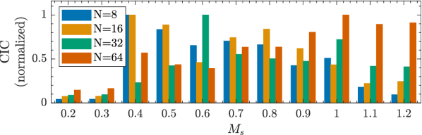
Figure 5. Average (over agents and trials) CIC values (normalized) vs. the equilibrium stock multiplier $M_{s}$, for population/signal size $N=G\in\{8,16,32,64\}$.

CIC values, averaged over agents and trials, vs. the equilibrium stock multiplier.

The results presented so far provide a qualitative measure of the influence of the introduced signal through the improvement on sustainability, social welfare, and convergence speed. They also indicate a decrease on the influence of the signal as resources become abundant. The question that naturally arises is: how much do agents actually take the signal into account in their policies? To answer this question, Fig. 5 depicts the CIC values – a quantitative measure of the influence of the introduced signal (see Section 3.1.5) – versus increasing values of $M_{s}$ (i.e, increasing $S_{eq}\propto M_{s}$, or more abundant resources), for population/signal size $N=G\in\{8,16,32,64\}$. The values are averaged across the 8 trials and the agents, and are normalized with respect to the maximum value for each population. Higher CIC values indicate a higher causal influence of the signal.

CIC is low for the trials in which a sustainable strategy could not be found ($M_{s}=0.2-0.3$ for $N=8$, $16$, $M_{s}=0.2-0.5$ for $N=32$, and $M_{s}=0.2-0.8$ for $N=64$, see Fig. 2(d)). In cases where a sustainable strategy was reached (e.g., $M_{s}\geq 0.4$ for $N=8$), we see significantly higher CIC values on scarce resource environments, and then the CIC decreases as $M_{s}$ increases. The harder the coordination problem, the more the agents rely on the environmental signal.

3.6. Robustness to Signal Size

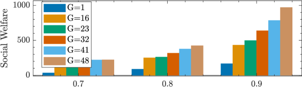
(a)

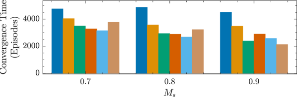
(b)

Figure 6. Achieved social welfare (Fig. 6(a)) and convergence time (Fig. 6(b)) for different signals of cardinality ($G$) $1$, $\frac{N}{2}=16$, $23$, $N=32$, $41$, and $\frac{3N}{2}=48$ (for varying resource levels $M_{s}$).

Achieved social welfare and convergence time for signal of different cardinality.

Up until now we have evaluated the presence (or lack thereof) of an environmental signal of cardinality equal to the population size ($G=N$). This requires exact knowledge of $N$, thus it is interesting to test the robustness of the proposed approach under varying signal sizes. As a representative test-case, we evaluated different signals of cardinality $G=1$, $\frac{N}{2}$, $23$, $N$, $41$, and $\frac{3N}{2}$ for $N=32$ and moderate scarcity for the resource ($M_{s}$ values of $0.7$, $0.8$ and $0.9$). The values $23$ and $41$ were chosen as they are prime numbers (i.e., not multiples of $N$). Fig. 6(b) depicts the achieved social welfare and convergence time under the aforementioned settings.

Starting with Fig. 6(a) we can see that the SW increases with the signal cardinality. Specifically, we have $263\%$, $255\%$, $341\%$, $416\%$, and $474\%$ improvement on average across the three $M_{s}$ values for $G=\frac{N}{2}$, $23$, $N$, $41$, and $\frac{3N}{2}$, respectively. We hypothesize that the improvement stems from an increased joint strategy space that the larger signal size allows. A signal size larger than $N$ can also allow the emergence of ‘rest’ (fallow) periods – signal values where the majority of agents harvests at really low efforts. This would allow the resource to recuperate, and increase the SW through a higher catchability coefficient. See Section 3.7 / Fig. 7(b) for an example.

Regarding the convergence speed (Fig. 6(b)), we have $22\%$, $38\%$, $36\%$, $41\%$, and $36\%$ improvement on average (across $M_{s}$ values).

These results showcase that the introduction of the signal itself – regardless of its cardinality or, more generally, its temporal representative power – provides a clear benefit to the agents in terms of SW and convergence speed. This greatly improves the real-world applicability of the proposed technique, as the the knowledge of the exact population size is not required; instead the agents can opt to select any signal available in their environment. Moreover, the signal cardinality can also be considered as a design choice, depending on the requirements and limitations of the system.

3.7. Emergence of Temporal Conventions

3.7.1. Qualitative Analysis

We have seen that the introduction of an arbitrary signal facilitates cooperation and the sustainable harvesting. But do temporal conventions actually emerge?

Fig. 7(a) presents an example of the evolution of the agents’ strategies for each signal value for a population of $N=4$, signal size $G=N=4$, and equilibrium stock multiplier $M_{s}=0.5$ (smoothed over 50 episodes). Each row represents an agent (agent $n_{i}$), while each column represents a signal value (value $g_{j}$). Each line represents the average effort the agent exerts on that specific signal value – calculated by averaging the actions of the agent in each corresponding signal value across the episode.

We can see a clear temporal convention emerging: at signal value $g_{1}$ (first column), only agents $n_{1}$ and $n_{3}$ harvest (first and third row), at $g_{2}$, $n_{2}$ and $n_{4}$ harvest, at $g_{3}$, $n_{1}$ and $n_{3}$ harvest, and, finally, at $g_{4}$, $n_{2}$ and $n_{4}$. Contrary to that, in a sustainable joint strategy without the use of the signal, every agent harvests at every time-step with an average (across all agents) effort of $\approx 40\%$ (for the same setting of $N=4$ and $M_{s}=0.5$). Having all agents harvesting at every time-step makes coordination increasingly harder as we increase the population size, mainly due to the non-stationarity of the environment (high variance) and the global exploration problem.

3.7.2. Access Rate

In order to facilitate a systematic analysis of the accessing patterns, we discretized the agents into three bins: agents harvesting with effort $\epsilon\in[0-0.33)$ (‘idle’), $[0.33-0.66)$ (‘moderate’), and $[0.66-1]$ (‘active’). Then we counted the average number of agents in each bin at the first equilibrium stock multiplier ($M_{s}$) where a non-depleting strategy was achieved in each setting. Without a signal, either the majority of the agents are ‘moderate’ harvesters (specifically $84\%$ for $N=8$ and $16$), or all of them are ‘active’ harvesters ($100\%$ for $N=32$ and $64$). With the signal, we have a clear separation into ‘idle’ and ‘active’: (‘idle’, ‘active’) = $(61\%,30\%)$, $(59\%,28\%)$, $(38\%,44\%)$, $(50\%,40\%)$, for $N=8$, $16$, $32$, and $64$, respectively. It is apparent that with the signal the agents learn a temporal convention; only a minority is ‘active’ per time-step, allowing to maintaining a healthy stock and reach sustainable strategies of high social welfare.

3.7.3. Fallowing

A more interesting joint strategy can be seen in Fig. 7(b) ($N=2$, $M_{s}=0.5$). In this setting, we have an increased number of available signals, specifically $G=\frac{3N}{2}=3$. We can see that agents harvest alternatingly in the first two signal values, and rest on the third (fallow period), potentially to allow resources to replenish and consequently obtain higher rewards in the future due to a higher catchability coefficient. This also resembles the optimal (bang-bang) harvesting strategy of Theorem 2.2.1.

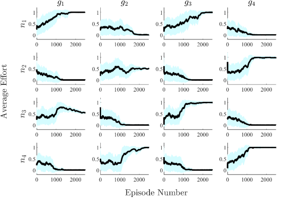
(a)

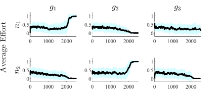
(b)

Figure 7. Evolution of the agents’ strategies for each signal value, smoothed over 50 episodes. Fig. 7(a) pertains to a population of $N=4$ and signal size $G=N=4$, while Fig. 7(b) to a population of $N=2$ and signal size $G=\frac{3N}{2}=3$. In both cases the equilibrium stock multiplier is $M_{s}=0.5$. Each row represents an agent ($n_{i}$), while each column a signal value ($g_{j}$). Each line depicts the average effort the agent exerts on that specific signal value – calculated by averaging the actions of the agent in each corresponding signal value across the episode. Shaded areas represent one standard deviation.

Evolution of the agents’ strategies for each signal value.

4. Conclusion

The challenge to cooperatively solve ‘the tragedy of the commons’ remains as relevant now as when it was first introduced by Hardin in 1968. Sustainable development and avoidance of catastrophic scenarios in socio-ecological systems – like the permanent depletion of resources, or the extinction of endangered species – constitute critical open problems. To add to the challenge, real-world problems are inherently large in scale and of low observability. This amplifies traditional problems in multi-agent learning, such as the global exploration and the moving-target problem. Earlier work in common-pool resource appropriation utilized intrinsic or extrinsic incentives (e.g., reward or opponent shaping). Yet, such techniques need to be designed for the problem at hand and/or require communication or observability of states/actions, which is not always feasible (e.g., in commercial fisheries, the stock or harvesting efforts can not be directly observed). Humans on the other hand show a remarkable ability to self-organize and resolve common-pool resource dilemmas, often without any extrinsic incentive mechanism or communication. Social conventions and the use of auxiliary environmental information constitute key mechanisms for the emergence of cooperation under low observability. In this paper, we demonstrate that utilizing such environmental signals – which are amply available – is a simple, yet powerful and robust technique, to foster cooperation in large-scale, low observability, and high-stakes environments. We are the first to tackle a realistic CPR appropriation scenario modeled on real-world commercial fisheries and under low observability. Our approach avoids permanent depletion in a wider (up to $300\%$) range of settings, while achieving higher social welfare (up to $3306\%$) and convergence speed (up to $53\%$).

Appendix A Appendix

A.1. Contents

In this appendix we include several details that have been omitted from the main text. In particular:

• In Section B, we prove Theorem 2.2.1.

• In Section C, we investigate the range of feasible values for the growth rate, $r$.

• In Section D, we provide details on the agent architecture, the introduced signal, the CIC metric, and the fairness indices.

• In Section E, we provide a thorough account of the simulation results.

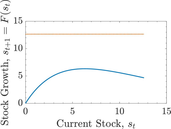
(a) $r=1$

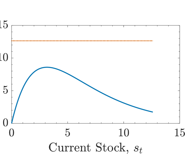
(b) $r=2$

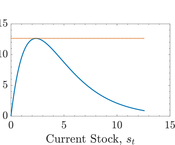
(c) $r=-W_{-1}(-\frac{1}{2e})\approx 2.678$

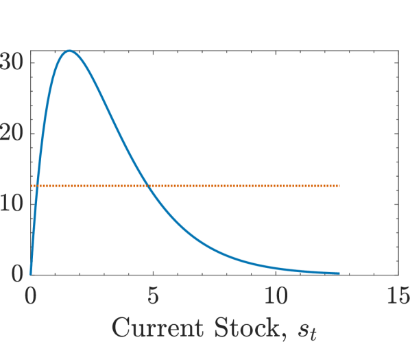
(d) $r=4$

Figure 8. Plot of the spawner-recruit function $F(\cdot)$ for various growth rates: $r=1$, $2$, $-W_{-1}(-\frac{1}{2e})\approx 2.678$, and $4$ (Fig. 8(a), 8(b), 8(c), and 8(d), respectively). The $x$-axis denotes the current stock level ($s_{t}$), while the $y$-axis depicts the stock level on the next time-step, assuming no harvest (i.e., $s_{t+1}=F(s_{t})$). The dashed line indicates a stock level equal to $2S_{eq}$.

Plot of the spawner-recruit function for various growth rates.

Appendix B Proof of Theorem 2.1

For completeness, we re-state the control problem and Theorem 2.2.1. We want to find a piecewise continuous control $E_{t}$, so as to maximize the total revenue for a given episode duration $T$ (Eq. 11, where $U_{t}(E_{t})$ is the cumulative revenue at time-step $t$, given by Eq. 12). The maximization problem can be solved using Optimal Control Theory Ding and Lenhart (2010); Lenhart and Workman (2007).

$$\begin{split}\underset{E_{t}}{\max}&\underset{t=0}{\overset{T}{\sum}}U_{t}(E_{t})\\ \text{subject to }s_{t+1}&=F(s_{t}-H(E_{t},s_{t}))\end{split}$$ (11)

$$U_{t}(E_{t})=p_{t}H(E_{t},s_{t})-c_{t}$$ (12)

The optimal control is given by the following theorem:

Theorem 2.1.

The optimal control variables $E^{*}_{t}$ that solves the maximization problem of Eq. 11 given the model dynamics described in Section 2.2 is given by the following equation, where $\lambda_{t}$ are the adjoint variables of the Hamiltonians:

$$E^{*}_{t+1}=\begin{cases}E_{max},&\text{if }(p_{t+1}-\lambda_{t+1})q(F(s_{t}-H(E_{t},s_{t})))\geq 0\\ 0,&\text{if }(p_{t+1}-\lambda_{t+1})q(F(s_{t}-H(E_{t},s_{t})))<0\\ \end{cases}$$

Proof.

In order to decouple the state ($s_{t}$, the current resource stock) and the control ($E_{t}$) and simplify the calculations, we resort to a change of variables. We define the new state $w_{t}$ as the remaining stock after harvest at time-step $t$:

$$w_{t}\triangleq s_{t}-H(E_{t},s_{t})$$

Therefore,

$$s_{t+1}=w_{t+1}+H(E_{t+1},s_{t+1})$$ (13)

and

$$s_{t+1}=F(s_{t}-H(E_{t},s_{t}))=F(w_{t})$$ (14)

Using Eq. 13 and 14, we can write the new state equation as:

$$w_{t+1}=F(w_{t})-H(E_{t+1},F(w_{t}))$$ (15)

In the current form of the state equation (Eq. 15), the harvested resources appear outside the nonlinear growth function $F(.)$, making the following analysis significantly simpler.

Under optimal control, the resource will not get depleted before the end of the horizon $T$, thus $q(s_{t})E_{t}\leq s_{t}$, $\forall t<T$. We can rewrite the total harvest as:

$$H(E_{t+1},F(w_{t}))=q(F(w_{t}))E_{t+1}$$ (16)

The state equation (Eq. 15) becomes:

$$w_{t+1}=F(w_{t})-q(F(w_{t}))E_{t+1}$$

and the optimization problem:

$$max\sum_{t=-1}^{T-1}(p_{t+1}q(F(w_{t}))E_{t+1}-c_{t+1})$$

$$subject\ to\ w_{t+1}=F(w_{t})-q(F(w_{t}))E_{t+1}$$

Let $w_{-1}=s_{0}=S_{eq}$. Solving the optimization problem is equivalent to finding the control that optimizes the Hamiltonians Lenhart and Workman (2007); Ding and Lenhart (2010). Let $\lambda=(\lambda_{-1},\lambda_{0},\dots,\lambda_{T-1})$ denote the adjoint function. The Hamiltonian at time-step $t$ is given by:

$$\begin{split}\textbf{H}_{t}&=p_{t+1}q(F(w_{t}))E_{t+1}-c_{t+1}+\lambda_{t+1}(F(w_{t})-q(F(w_{t}))E_{t+1})\\ &=(p_{t+1}-\lambda_{t+1})q(F(w_{t}))E_{t+1}-c_{t+1}+\lambda_{t+1}F(w_{t})\end{split}$$ (17)

The adjoint equations are given by Ding and Lenhart (2010):

$$\begin{split}\lambda_{t}&=\frac{\partial\mathbf{H}_{t}}{\partial w_{t}}\\ \lambda_{T}&=0\\ \frac{\partial\mathbf{H}_{t}}{\partial u_{t}}&=0\ \textup{at}\ u_{t}=u^{*}_{t}\end{split}$$

where $u_{t}$ is the control input, which corresponds to $E_{t+1}$ in our formulation. The last condition corresponds to the maximization of the Hamiltonian $\textbf{H}_{t}$ in Eq. 17 for all time-steps $t$ (Lenhart and Workman, 2007, Chapter 23). In our case, Eq. 17 is linear in $E_{t+1}$ with coefficient $(p_{t+1}-\lambda_{t+1})q(F(w_{t}))$. Therefore, the optimal sequence of $E_{t+1}$ that maximizes Eq. 17 is given based on the sign of the coefficient:

$$E^{*}_{t+1}=\begin{cases}E_{max},&\text{if }(p_{t+1}-\lambda_{t+1})q(F(w_{t}))\geq 0\\ 0,&\text{if }(p_{t+1}-\lambda_{t+1})q(F(w_{t}))<0\\ \end{cases}$$

The optimal strategy therefore implements bang–bang controller, which oscillates based on adjoint variable values $\lambda_{t}$, current state $w_{t}$, and price $p_{t}$.

∎

Appendix C Growth Rate

The growth rate, $r$, plays a significant role in the stability of the stock dynamics. A high growth rate – and subsequently high population density – can even lead to the extinction of the population due to the collapse in behavior from overcrowding (a phenomenon known as ‘behavioral sink’ Calhoun (1962, 1973)). This is reflected by the spawner-recruit function (Eq. 4) in our model. As depicted in Fig. 8(d), the higher the growth rate, $r$, the more skewed the stock dynamics. Specifically, Fig. 8(d) plots the spawner-recruit function $F(\cdot)$ for various growth rates: $r=1$, $2$, $-W_{-1}(-\frac{1}{2e})\approx 2.678$, and $4$ (Fig. 8(a), 8(b), 8(c), and 8(d), respectively). The $x$-axis denotes the current stock level ($s_{t}$), while the $y$-axis depicts the stock level on the next time-step, assuming no harvest (i.e., $s_{t+1}=F(s_{t})$). The dashed line indicates a stock level equal to $2S_{eq}$. For a growth rate of $r=4$ for example (Fig. 8(d)), we have a highly skewed growth model that can lead to the depletion of the resource (high stock values ($s_{t}$) result to $s_{t+1}<\delta\rightarrow 0$, i.e., permanent depletion of the resource). For this reason, we want an unskewed growth model, specifically we want the stock to remain below two times the equilibrium stock point, i.e., $s_{t+1}\leq 2S_{eq}$. For this reason, we need to bound the growth rate according to the following theorem:

For a continuous resource governed by the dynamics of Section 2.2, the stock value does not exceed the limit of $2S_{eq}$, if $r\in[-W(-1/(2e)),-W_{-1}(-1/(2e))]\approx[0.232,2.678]$, where $W_{k}(\cdot)$ is the Lambert $W$ function.

Proof.

Let $x\triangleq s_{t}\leq 2S_{eq}$ for a time-step $t$. We want $s_{t+1}\leq 2S_{eq}$, thus we need to bound the maximum value of the spawner-recruit function, $F(x)$ (Eq. 4).

Taking the derivative:

$$\frac{\partial}{\partial x}F(x)=e^{r\left(1-\frac{x}{S_{eq}}\right)}\left(1-\frac{rx}{S_{eq}}\right)$$

We have that:

$$\frac{\partial}{\partial x}F(x)=0\Rightarrow x=\frac{S_{eq}}{r},r\neq 0\text{ and }S_{eq}\neq 0$$

Thus the maximum value is:

$$F\left(\frac{S_{eq}}{r}\right)=\frac{S_{eq}}{r}e^{(r-1)}$$

We want to bound the maximum value:

$$\begin{split}F\left(\frac{S_{eq}}{r}\right)\leq 2S_{eq}&\Rightarrow\frac{e^{(r-1)}}{r}\leq 2\Rightarrow e^{r}-2er\leq 0\\ &\Rightarrow-W\left(-\frac{1}{2e}\right)\leq r\leq-W_{-1}\left(-\frac{1}{2e}\right)\end{split}$$

where $W_{k}(\cdot)$ is the Lambert $W$ function. $-W(-1/(2e))\approx 0.232$ and $-W_{-1}(-1/(2e))\approx 2.678$. ∎

Appendix D Modeling Details

D.1. Agent Architecture Details

Recent work has demonstrated that code-level optimizations play an important role in performance, both in terms of achieved reward and underlying algorithmic behavior Engstrom et al. (2020). To minimize those sources of stochasticity – and given that the focus of this work is in the performance of the introduced technique and not of the training algorithm – we opted to use RLlib as our implementation framework. Each agent uses a two-layer ($64$ neurons each) feed-forward neural network for the policy approximation. The policies are trained using the Proximal Policy Optimization (PPO) algorithm Schulman et al. (2017). All the hyper-parameters were left to the default values specified in Ray and RLlib. For completeness, Table 1 presents a list of the most relevant of them.

Table 1. List of hyper-parameters.

Parameter	Value
Learning Rate ($\alpha$)	0.0001
Clipping Parameter	0.3
Value Function Clipping Parameter	10.0
KL Target	0.01
Discount Factor ($\gamma$)	0.99
GAE Parameter Lambda	1.0
Value Function Loss Coefficient	1.0
Entropy Coefficient	0.0

D.2. Introduced Signal: Implementation Details

The introduced signal was encoded as a $G$-dimensional one-hot vector of fixed size, in which the high bit is shifted periodically. In particular, its value at index $i$ at time-step $t$ is given by:

$$\begin{cases}1&\text{if }mod(t-t_{init},\ G)=i\\ 0&\text{otherwise}\\ \end{cases}$$ (18)

where $t_{init}$ is the random offset determined at the beginning of each episode in order to avoid learning any bias towards certain signal values.

D.3. Causal Influence of Communication (CIC): Implementation Details

The Causal Influence of Communication (CIC) Lowe et al. (2019) estimates the mutual information between the signal and the agent’s action. The mutual information between two random variables $\tilde{X}$ and $\tilde{Y}$ is defined as the reduction of uncertainty (measured in terms of entropy $H_{S}(\cdot)$) in the value of $\tilde{X}$ with the observation of $\tilde{Y}$:

$$I(\tilde{X},\tilde{Y})=I(\tilde{Y},\tilde{X})=H_{S}(\tilde{X})-H_{S}(\tilde{X}|\tilde{Y})=E\left\{log\left(\frac{P_{\tilde{X},\tilde{Y}}(\tilde{x},\tilde{y})}{P_{\tilde{X}}(\tilde{x})P_{\tilde{Y}}(\tilde{y})}\right)\right\}$$

The pseudo-code for calculating the CIC for a single agent is presented in Alg. 1. Note that the CIC implementation in Lowe et al. (2019) considers a multi-dimensional, one-hot, discrete action space with accessible probabilities for every action, while in our case we have a single, continuous action (specifically, the effort $\epsilon_{n,t}$). To solve this problem, we discretize our action space into $N_{bins}$ intervals between minimum ($\mathcal{E}_{min}=0$) and maximum ($\mathcal{E}_{max}=1$) effort values, and each interval is assumed to correspond to a single discrete action. Let $a_{i}$ denote the event of an action $\epsilon_{n,t}$ belonging to interval $i$. To calculate the CIC value, we start by generating $N_{states}$ random ‘partial’ states (i.e., without signal), $\sigma_{-g}$, which are then concatenated with each possible signal value to obtain a ‘complete’ state, $\sigma=[g_{j},\sigma_{-g}]$ (Lines 5 - 7 of Alg. 1). Then, we estimate the probability of an action given a signal value, $p(a_{i}|g_{j})$, by generating $N_{samples}$ actions from our policy given the ‘complete’ state ($\pi(\sigma)$), and normalizing the number of instances in which the action belongs to a particular bin with the total number of samples. The remaining aspects of the calculation are the same as in the original implementation. In our calculations we used $N_{states}=N_{samples}=100$.

1

2input: Agent policy $\pi(\cdot)$

3$p(g_{j})=\frac{1}{G}$ for all possible signals

4Discretize the action space $[0,\mathcal{E}_{max}]$ into $N_{bins}$ intervals.

5for i=1 to $N_{states}$ do

6       Generate a state without a signal $\sigma_{-g}$ randomly

7      for all possible signals $g_{j}$ do

8             Generate agent observation $\sigma=[g_{j},\sigma_{-g}]$

9            Estimate $p(a_{i}|g_{j})$ by sampling $N_{samples}$ actions from $\pi(\sigma)$

10            $p(a_{i},g_{j})=p(a_{i}|g_{j})p(g_{j})$

11       end for

12      $p(a_{i})=\sum_{j}p(a,g_{j})$

13      $CIC+=\frac{1}{N_{states}}\sum_{a_{i}|p(a_{i})\neq 0,\ g_{j}}p(a,g_{j})log(\frac{p(a,g_{j})}{p(a)p(g_{j})})$

14 end for

Algorithm 1 CIC Implementation (based on Lowe et al. (2019))

D.4. Fairness Metrics

We also evaluated the fairness of the final allocation, to ensure that agents are not being exploited by the introduction of the signal. We used two of most established fairness metrics: the Jain index Jain et al. (1998) and the Gini coefficient Gini (1912):

(a) The Jain index Jain et al. (1998): Widely used in network engineering to determine whether users or applications receive a fair share of system resources. It exhibits a lot of desirable properties such as: population size independence, continuity, scale and metric independence, and boundedness. For an allocation of $N$ agents, such that the $n^{\text{th}}$ agent is alloted $x_{n}$, the Jain index is given by Eq. 19. $\mathds{J}(\mathbf{x})\in[0,1]$. An allocation $\mathbf{x}=(x_{1},\dots,x_{N})^{\top}$ is considered fair, iff $\mathds{J}(\mathbf{x})=1$.

$$\mathds{J}(\mathbf{x})=\frac{\left(\underset{n=1}{\overset{N}{\sum}}x_{n}\right)^{2}}{N\underset{n=1}{\overset{N}{\sum}}x_{n}^{2}}$$ (19)

(b) The Gini coefficient Gini (1912): One of the most commonly used measures of inequality by economists intended to represent the wealth distribution of a population of a nation. For an allocation game of $N$ agents, such that the $n^{\text{th}}$ agent is alloted $x_{n}$, the Gini coefficient is given by Eq. 20. $\mathds{G}(\mathbf{x})\geq 0$. A Gini coefficient of zero expresses perfect equality, i.e., an allocation is fair iff $\mathds{G}(\mathbf{x})=0$.

$$\mathds{G}(\mathbf{x})=\frac{\underset{n=1}{\overset{N}{\sum}}\underset{n^{\prime}=1}{\overset{N}{\sum}}\left|x_{n}-x_{n^{\prime}}\right|}{2N\underset{n=1}{\overset{N}{\sum}}x_{n}}$$ (20)

Both metrics showed that learning both with and without the signal results in fair allocations, with no significant change with the introduction of the signal (see Section E).

Appendix E Simulation Results in Detail

In this section we provide numerical values of the simulation results presented in the main text. Specifically:

Tables (2 and 3), (4 and 5), (6 and 7), (8 and 9), and (10 and 11) include the results (absolute values with and without the introduced signal, relative difference, and Student’s T-test p-values) on social welfare, episode lengths (in time-steps), training time (in number of episodes), Jain index, and Gini coefficient, respectively.

Table 12 presents the CIC values.

Tables 13, 14, 15, 16, and 17 present the results on the aforementioned metrics for varying signal size, $G=\{1,\frac{N}{2},23,N,41,\frac{3N}{2}\}$.

We also ran simulations with higher growth rate, specifically $r=2$. The results can be found in Tables 18, and 19. Every resource has a natural upper limit on the size of the population it can sustain. Fig. 2(d) shows that as the number of agents grow, we reach sustainable strategies at higher equilibrium stock multipliers ($M_{s}$). Thus, we expect that as we increase the growth rate, the effect of the signal will be even more pronounced in larger populations ($N$) – which is corroborated by the aforementioned Tables. The environment’s ability to sustain a population also affects the counts of ‘active’ agents of Section 3.7.2. As we can see in Fig. 2(d), for a growth rate of $r=1$, the resource is too scarce, thus, even with the addition of the signal, the first sustainable strategy is reached at $M_{s}=0.9$. This is a high equilibrium stock multiplier, close to the limit of sustainable harvesting. As a result, the number of ‘active’ agents is naturally really high because they do not need to harvest in turns. By increasing the growth rate to $r=2$, we have an environment that can sustain larger populations. Therefore, the first strategy that does not result to an immediate depletion is reached much earlier, and we can observe the emergence of a temporal convention (see Table 20).

Finally, Table 20 shows the average number of agents in each bin – $\epsilon\in[0-0.33)$ (‘idle’), $[0.33-0.66)$ (‘moderate’), and $[0.66-1]$ (‘active’) – starting from the first equilibrium stock multiplier ($M_{s}$) where a non-depleting strategy was achieved in each setting.

All reported results are the average values over 8 trials. Note also that, as was specified in Section 3.1.1, $K=\frac{S^{\scriptscriptstyle N,r}_{\scriptscriptstyle LSH}}{N}=\frac{e^{r}\mathcal{E}_{max}}{2(e^{r}-1)}$. Therefore, in the settings where the growth rate is $r=1$, $K\approx 0.79$, while in the settings where $r=2$, $K\approx 0.58$.

Table 2. Social Welfare
Results (averaged over 8 trials) for increasing population size ($N\in[2,64]$), with ($G=N$) and without ($G=1$) the introduced signal, for environments of decreasing difficulty (increasing $S_{eq}\propto M_{s}$).

	$N=$2		$N=4$		$N=8$		$N=16$		$N=32$		$N=64$
	$G=1$	$G=N$	$G=1$	$G=N$	$G=1$	$G=N$	$G=1$	$G=N$	$G=1$	$G=N$	$G=1$	$G=N$
$M_{s}=0.2$	0.36	0.36	0.76	0.76	1.50	1.51	2.92	2.92	5.65	5.65	10.96	10.96
$M_{s}=0.3$	0.60	0.60	1.28	1.28	2.64	2.64	5.38	4.81	8.26	8.61	16.38	15.29
$M_{s}=0.4$	3.68	43.46	2.30	2.89	4.70	160.05	5.77	130.37	10.66	10.73	20.45	21.10
$M_{s}=0.5$	122.30	111.57	179.20	186.65	141.89	193.53	70.10	154.00	12.81	39.35	25.67	25.81
$M_{s}=0.6$	143.23	135.73	206.14	232.03	174.52	215.93	176.30	157.74	15.20	130.34	30.37	33.12
$M_{s}=0.7$	172.69	179.28	181.15	223.18	121.33	211.70	196.26	202.63	34.14	196.57	41.49	52.57
$M_{s}=0.8$	176.33	199.11	200.64	275.35	200.10	291.44	247.90	304.74	86.95	316.08	62.28	80.49
$M_{s}=0.9$	197.49	207.15	244.93	316.75	327.91	395.14	341.24	499.66	165.75	637.30	101.12	1517.30
$M_{s}=1.0$	223.28	229.01	339.33	371.72	482.25	524.64	585.71	687.65	592.26	1717.98	297.34	5350.52
$M_{s}=1.1$	252.41	250.56	418.38	429.24	674.72	707.17	1315.68	1348.68	2611.96	3415.66	5225.12	8317.41
$M_{s}=1.2$	280.61	278.61	523.86	532.54	1046.36	1051.10	2091.35	2120.13	4180.33	4784.53	8367.87	9900.67

Table 3. Social Welfare (Relative difference & p-values)
(i) Relative difference in Social Welfare when signal of cardinality $G=N$ is introduced ($(\text{Result}_{G=N}-\text{Result}_{G=1})/\text{Result}_{G=1}$, where $\text{Result}_{G=X}$ denotes the achieved result using a signal of cardinality $X$), and
(ii) Student’s T-test p-values,
for varying population size ($N\in[2,64]$) and environments of decreasing difficulty (increasing $S_{eq}\propto M_{s}$).

	$N=$2		$N=4$		$N=8$		$N=16$		$N=32$		$N=64$
	(%)	p	(%)	p	(%)	p	(%)	p	(%)	p	(%)	p
$M_{s}=0.2$	0.0	0.87876	0.2	0.57508	0.2	0.47454	-0.1	0.47064	0.1	0.36608	0.0	0.93297
$M_{s}=0.3$	-0.3	0.48043	0.2	0.57516	0.1	0.82779	-10.5	0.02451	4.2	0.00000	-6.6	0.00000
$M_{s}=0.4$	1082.1	0.01102	25.8	0.16861	3305.9	0.00000	2158.1	0.00000	0.7	0.74501	3.2	0.01327
$M_{s}=0.5$	-8.8	0.00453	4.2	0.42501	36.4	0.00261	119.7	0.00566	207.2	0.14710	0.6	0.48706
$M_{s}=0.6$	-5.2	0.01401	12.6	0.01795	23.7	0.00033	-10.5	0.48519	757.6	0.00001	9.1	0.00000
$M_{s}=0.7$	3.8	0.00161	23.2	0.00000	74.5	0.00000	3.2	0.83672	475.7	0.00000	26.7	0.00000
$M_{s}=0.8$	12.9	0.00032	37.2	0.00013	45.6	0.00105	22.9	0.00886	263.5	0.00000	29.2	0.00000
$M_{s}=0.9$	4.9	0.06719	29.3	0.00008	20.5	0.12549	46.4	0.00355	284.5	0.00000	1400.5	0.00000
$M_{s}=1.0$	2.6	0.03517	9.5	0.02099	8.8	0.01232	17.4	0.00014	190.1	0.00000	1699.5	0.00000
$M_{s}=1.1$	-0.7	0.41309	2.6	0.12172	4.8	0.01402	2.5	0.00002	30.8	0.00000	59.2	0.00000
$M_{s}=1.2$	-0.7	0.56215	1.7	0.00477	0.5	0.09644	1.4	0.00000	14.5	0.00000	18.3	0.00000

Table 4. Episode Length (#time-steps)
Results (averaged over 8 trials) for increasing population size ($N\in[2,64]$), with ($G=N$) and without ($G=1$) the introduced signal, for environments of decreasing difficulty (increasing $S_{eq}\propto M_{s}$).

	$N=$2		$N=4$		$N=8$		$N=16$		$N=32$		$N=64$
	$G=1$	$G=N$	$G=1$	$G=N$	$G=1$	$G=N$	$G=1$	$G=N$	$G=1$	$G=N$	$G=1$	$G=N$
$M_{s}=0.2$	2.04	2.04	2.14	2.14	2.05	2.06	2.01	2.01	1.99	2.00	1.96	1.96
$M_{s}=0.3$	2.75	2.72	2.83	2.82	3.63	3.66	5.17	3.61	1.98	2.67	2.20	1.19
$M_{s}=0.4$	25.17	276.52	6.50	8.50	11.26	491.08	6.15	474.22	2.25	1.95	1.44	2.07
$M_{s}=0.5$	499.79	499.94	463.01	500.00	481.93	500.00	240.27	496.08	1.90	119.85	2.62	2.32
$M_{s}=0.6$	499.98	499.96	498.51	499.49	499.90	499.72	499.85	495.69	2.36	438.24	2.72	6.78
$M_{s}=0.7$	500.00	500.00	499.24	500.00	499.49	500.00	500.00	500.00	70.78	500.00	10.00	31.33
$M_{s}=0.8$	500.00	500.00	500.00	500.00	500.00	500.00	500.00	500.00	200.63	500.00	22.00	66.68
$M_{s}=0.9$	500.00	500.00	500.00	500.00	500.00	500.00	500.00	500.00	275.00	500.00	53.00	500.00
$M_{s}=1.0$	500.00	500.00	500.00	500.00	500.00	500.00	500.00	500.00	500.00	500.00	500.00	500.00
$M_{s}=1.1$	500.00	500.00	500.00	500.00	500.00	500.00	500.00	500.00	500.00	500.00	500.00	500.00
$M_{s}=1.2$	500.00	500.00	500.00	500.00	500.00	500.00	500.00	500.00	500.00	500.00	500.00	500.00

Table 5. Episode Length (Relative difference & p-values)
(i) Relative difference in Episode Length when signal of cardinality $G=N$ is introduced ($(\text{Result}_{G=N}-\text{Result}_{G=1})/\text{Result}_{G=1}$, where $\text{Result}_{G=X}$ denotes the achieved result using a signal of cardinality $X$), and
(ii) Student’s T-test p-values,
for varying population size ($N\in[2,64]$) and environments of decreasing difficulty (increasing $S_{eq}\propto M_{s}$).
NaN values in the p-values column are due to having only a single data point; both cases (with and without the signal) have the same episode length in all the trials.

	$N=$2		$N=4$		$N=8$		$N=16$		$N=32$		$N=64$
	(%)	p	(%)	p	(%)	p	(%)	p	(%)	p	(%)	p
$M_{s}=0.2$	0.0	0.99280	0.0	0.98122	0.7	0.43808	-0.5	0.34488	0.6	0.32379	0.0	0.97624
$M_{s}=0.3$	-0.9	0.37060	-0.2	0.83869	0.9	0.48086	-30.2	0.02482	34.7	0.00000	-46.0	0.00000
$M_{s}=0.4$	998.6	0.00924	30.7	0.16075	4261.1	0.00000	7610.6	0.00000	-13.3	0.52170	44.2	0.04255
$M_{s}=0.5$	0.0	0.36593	8.0	0.04688	3.8	0.20338	106.5	0.01043	6209.4	0.14849	-11.8	0.56968
$M_{s}=0.6$	0.0	0.58271	0.2	0.36518	0.0	0.56152	-0.8	0.02847	18503.0	0.00001	149.4	0.00001
$M_{s}=0.7$	0.0	NaN	0.2	0.13837	0.1	0.10198	0.0	NaN	606.4	0.00001	213.3	0.00000
$M_{s}=0.8$	0.0	NaN	0.0	NaN	0.0	NaN	0.0	NaN	149.2	0.00418	203.1	0.00000
$M_{s}=0.9$	0.0	NaN	0.0	NaN	0.0	NaN	0.0	NaN	81.8	0.01919	843.4	0.00000
$M_{s}=1.0$	0.0	NaN	0.0	NaN	0.0	NaN	0.0	NaN	0.0	NaN	0.0	NaN
$M_{s}=1.1$	0.0	NaN	0.0	NaN	0.0	NaN	0.0	NaN	0.0	NaN	0.0	NaN
$M_{s}=1.2$	0.0	NaN	0.0	NaN	0.0	NaN	0.0	NaN	0.0	NaN	0.0	NaN

Table 6. Training Time (#episodes)
Results (averaged over 8 trials) for increasing population size ($N\in[2,64]$), with ($G=N$) and without ($G=1$) the introduced signal, for environments of decreasing difficulty (increasing $S_{eq}\propto M_{s}$).

	$N=$2		$N=4$		$N=8$		$N=16$		$N=32$		$N=64$
	$G=1$	$G=N$	$G=1$	$G=N$	$G=1$	$G=N$	$G=1$	$G=N$	$G=1$	$G=N$	$G=1$	$G=N$
$M_{s}=0.2$	5000.00	5000.00	5000.00	5000.00	5000.00	5000.00	5000.00	5000.00	5000.00	5000.00	5000.00	5000.00
$M_{s}=0.3$	5000.00	5000.00	5000.00	5000.00	5000.00	5000.00	5000.00	5000.00	5000.00	5000.00	5000.00	5000.00
$M_{s}=0.4$	5000.00	5000.00	5000.00	5000.00	5000.00	4990.13	5000.00	4960.13	5000.00	5000.00	5000.00	5000.00
$M_{s}=0.5$	4955.38	4340.63	4971.25	3408.75	5000.00	3389.50	5000.00	4847.88	5000.00	5000.00	5000.00	5000.00
$M_{s}=0.6$	3037.38	2268.00	3822.75	2013.75	3903.00	3051.63	4583.13	2797.50	5000.00	4081.13	5000.00	5000.00
$M_{s}=0.7$	1536.13	1008.13	2478.63	1328.00	3104.50	1880.00	3213.00	2680.00	4937.00	3026.00	5000.00	5000.00
$M_{s}=0.8$	1004.00	1124.00	1968.00	1296.00	3088.00	2064.00	3778.00	2116.00	4887.00	2551.00	5000.00	5000.00
$M_{s}=0.9$	1248.00	936.00	2168.00	1416.00	3025.00	1412.00	3810.00	2100.00	4536.00	2896.00	5000.00	2581.00
$M_{s}=1.0$	864.00	776.00	1692.00	1252.00	2116.00	1612.00	2740.00	1788.00	3393.00	2334.00	1484.00	1965.00
$M_{s}=1.1$	684.00	800.00	1028.00	1376.00	1284.00	1436.00	1164.00	1536.00	1218.00	1832.00	1193.00	1172.00
$M_{s}=1.2$	840.00	780.00	1132.00	1040.00	1004.00	1212.00	932.00	1116.00	949.00	844.00	897.00	816.00

Table 7. Training Time (Relative difference & p-values)
(i) Relative difference in Training Time when signal of cardinality $G=N$ is introduced ($(\text{Result}_{G=N}-\text{Result}_{G=1})/\text{Result}_{G=1}$, where $\text{Result}_{G=X}$ denotes the achieved result using a signal of cardinality $X$), and
(ii) Student’s T-test p-values,
for varying population size ($N\in[2,64]$) and environments of decreasing difficulty (increasing $S_{eq}\propto M_{s}$).

	$N=$2		$N=4$		$N=8$		$N=16$		$N=32$		$N=64$
	(%)	p	(%)	p	(%)	p	(%)	p	(%)	p	(%)	p
$M_{s}=0.2$	0.0	0.00000	0.0	0.00000	0.0	0.00000	0.0	0.00000	0.0	0.00000	0.0	0.00000
$M_{s}=0.3$	0.0	0.00000	0.0	0.00000	0.0	0.00000	0.0	0.00000	0.0	0.00000	0.0	0.00000
$M_{s}=0.4$	0.0	0.00000	0.0	0.00000	-0.2	0.00000	-0.8	0.00000	0.0	0.00000	0.0	0.00000
$M_{s}=0.5$	-12.4	0.00000	-31.4	0.00000	-32.2	0.00000	-3.0	0.00000	0.0	0.00000	0.0	0.00000
$M_{s}=0.6$	-25.3	0.00000	-47.3	0.00006	-21.8	0.00013	-39.0	0.00003	-18.4	0.00000	0.0	0.00000
$M_{s}=0.7$	-34.4	0.00000	-46.4	0.02193	-39.4	0.00396	-16.6	0.00666	-38.7	0.00000	0.0	0.00000
$M_{s}=0.8$	12.0	0.01448	-34.1	0.00266	-33.2	0.00228	-44.0	0.00128	-47.8	0.00000	0.0	0.00000
$M_{s}=0.9$	-25.0	0.00462	-34.7	0.01569	-53.3	0.00583	-44.9	0.00221	-36.2	0.00001	-48.4	0.00000
$M_{s}=1.0$	-10.2	0.00137	-26.0	0.02400	-23.8	0.01508	-34.7	0.03351	-31.2	0.00211	32.4	0.00000
$M_{s}=1.1$	17.0	0.00000	33.9	0.00024	11.8	0.00006	32.0	0.00000	50.4	0.00001	-1.8	0.00000
$M_{s}=1.2$	-7.1	0.00847	-8.1	0.00002	20.7	0.00000	19.7	0.00000	-11.1	0.00000	-9.0	0.00000

Table 8. Jain Index (higher is fairer)
Results (averaged over 8 trials) for increasing population size ($N\in[2,64]$), with ($G=N$) and without ($G=1$) the introduced signal, for environments of decreasing difficulty (increasing $S_{eq}\propto M_{s}$).

	$N=$2		$N=4$		$N=8$		$N=16$		$N=32$		$N=64$
	$G=1$	$G=N$	$G=1$	$G=N$	$G=1$	$G=N$	$G=1$	$G=N$	$G=1$	$G=N$	$G=1$	$G=N$
$M_{s}=0.2$	0.99984	0.99973	0.99976	0.99984	0.99963	0.99966	0.99967	0.99961	0.99943	0.99947	0.99932	0.99941
$M_{s}=0.3$	0.99973	0.99991	0.99984	0.99981	0.99967	0.99974	0.99963	0.99959	0.99958	0.99930	0.99936	0.99942
$M_{s}=0.4$	0.99210	0.99299	0.99910	0.99846	0.99119	0.98808	0.98691	0.99370	0.98603	0.99526	0.99063	0.99648
$M_{s}=0.5$	0.98061	0.98251	0.97149	0.97895	0.97910	0.98978	0.98376	0.99416	0.98946	0.99694	0.99489	0.99773
$M_{s}=0.6$	0.98252	0.99911	0.98507	0.99479	0.97847	0.99246	0.98147	0.99599	0.99898	0.99628	0.99935	0.99831
$M_{s}=0.7$	0.99317	0.99996	0.98657	0.99239	0.98647	0.99458	0.98862	0.99601	0.99635	0.99660	1.00000	0.99787
$M_{s}=0.8$	0.99705	0.99872	0.98081	0.99269	0.97903	0.99534	0.98679	0.99645	0.99023	0.99733	1.00000	0.99864
$M_{s}=0.9$	0.99780	0.99535	0.97744	0.99304	0.97841	0.99581	0.98236	0.99704	0.99234	0.99810	0.99999	0.99912
$M_{s}=1.0$	0.98674	0.99740	0.98892	0.99454	0.99094	0.99715	0.99441	0.99876	0.99578	0.99924	1.00000	0.99929
$M_{s}=1.1$	0.99620	0.99498	0.99770	0.99737	0.99990	0.99976	0.99999	0.99999	1.00000	0.99945	0.99999	0.99909
$M_{s}=1.2$	0.99855	0.99956	0.99998	0.99993	0.99999	0.99999	1.00000	0.99998	0.99999	0.99917	0.99999	0.99876

Table 9. Jain Index (Relative difference & p-values)
(i) Relative difference in Jain Index when signal of cardinality $G=N$ is introduced ($(\text{Result}_{G=N}-\text{Result}_{G=1})/\text{Result}_{G=1}$, where $\text{Result}_{G=X}$ denotes the achieved result using a signal of cardinality $X$), and
(ii) Student’s T-test p-values,
for varying population size ($N\in[2,64]$) and environments of decreasing difficulty (increasing $S_{eq}\propto M_{s}$).

	$N=$2		$N=4$		$N=8$		$N=16$		$N=32$		$N=64$
	(%)	p	(%)	p	(%)	p	(%)	p	(%)	p	(%)	p
$M_{s}=0.2$	0.0	0.62689	0.0	0.19181	0.0	0.73995	0.0	0.43584	0.0	0.67344	0.0	0.12180
$M_{s}=0.3$	0.0	0.19431	0.0	0.74755	0.0	0.40216	0.0	0.68556	0.0	0.00316	0.0	0.24335
$M_{s}=0.4$	0.1	0.85540	-0.1	0.47459	-0.3	0.31067	0.7	0.00312	0.9	0.00014	0.6	0.00000
$M_{s}=0.5$	0.2	0.88279	0.8	0.27542	1.1	0.08226	1.1	0.00027	0.8	0.00105	0.3	0.00025
$M_{s}=0.6$	1.7	0.05974	1.0	0.02806	1.4	0.00501	1.5	0.00055	-0.3	0.00000	-0.1	0.00000
$M_{s}=0.7$	0.7	0.16061	0.6	0.25648	0.8	0.00610	0.7	0.00002	0.0	0.94743	-0.2	0.00000
$M_{s}=0.8$	0.2	0.33436	1.2	0.03393	1.7	0.00015	1.0	0.00049	0.7	0.16118	-0.1	0.00000
$M_{s}=0.9$	-0.2	0.36223	1.6	0.00338	1.8	0.00011	1.5	0.00000	0.6	0.07503	-0.1	0.00000
$M_{s}=1.0$	1.1	0.07827	0.6	0.08720	0.6	0.00834	0.4	0.00017	0.3	0.00165	-0.1	0.00000
$M_{s}=1.1$	-0.1	0.49041	0.0	0.64625	0.0	0.11982	0.0	0.18597	-0.1	0.00006	-0.1	0.00000
$M_{s}=1.2$	0.1	0.05751	0.0	0.15660	0.0	0.38672	0.0	0.00003	-0.1	0.00000	-0.1	0.00000

Table 10. Gini Coefficient (lower is fairer)
Results (averaged over 8 trials) for increasing population size ($N\in[2,64]$), with ($G=N$) and without ($G=1$) the introduced signal, for environments of decreasing difficulty (increasing $S_{eq}\propto M_{s}$).

	$N=$2		$N=4$		$N=8$		$N=16$		$N=32$		$N=64$
	$G=1$	$G=N$	$G=1$	$G=N$	$G=1$	$G=N$	$G=1$	$G=N$	$G=1$	$G=N$	$G=1$	$G=N$
$M_{s}=0.2$	0.00583	0.00551	0.00764	0.00663	0.01048	0.00956	0.00991	0.01087	0.01323	0.01282	0.01459	0.01356
$M_{s}=0.3$	0.00674	0.00390	0.00644	0.00656	0.00983	0.00855	0.01040	0.01085	0.01135	0.01468	0.01416	0.01345
$M_{s}=0.4$	0.03897	0.03083	0.01409	0.01667	0.05032	0.05879	0.06336	0.04329	0.06617	0.03841	0.05399	0.03328
$M_{s}=0.5$	0.05571	0.05590	0.08869	0.07415	0.07528	0.05419	0.06839	0.04166	0.05646	0.03109	0.03890	0.02668
$M_{s}=0.6$	0.05350	0.01113	0.06094	0.03547	0.07879	0.04711	0.07156	0.03444	0.01466	0.03405	0.01272	0.02298
$M_{s}=0.7$	0.02754	0.00215	0.05777	0.04123	0.06279	0.03842	0.05894	0.03514	0.01252	0.03259	0.00038	0.02537
$M_{s}=0.8$	0.02160	0.01446	0.07129	0.04442	0.07916	0.03539	0.06264	0.03255	0.03503	0.02884	0.00012	0.02059
$M_{s}=0.9$	0.01901	0.02562	0.08016	0.03768	0.07998	0.03427	0.07229	0.02973	0.03275	0.02440	0.00027	0.01639
$M_{s}=1.0$	0.04736	0.02190	0.05277	0.03522	0.04490	0.02877	0.03175	0.01899	0.01802	0.01524	0.00012	0.01480
$M_{s}=1.1$	0.02741	0.03299	0.02376	0.02583	0.00392	0.00692	0.00119	0.00191	0.00035	0.01244	0.00038	0.01670
$M_{s}=1.2$	0.01585	0.00951	0.00138	0.00358	0.00102	0.00154	0.00078	0.00235	0.00083	0.01604	0.00113	0.01958

Table 11. Gini Coefficient (Relative difference & p-values)
(i) Relative difference in Gini Coefficient when signal of cardinality $G=N$ is introduced ($(\text{Result}_{G=N}-\text{Result}_{G=1})/\text{Result}_{G=1}$, where $\text{Result}_{G=X}$ denotes the achieved result using a signal of cardinality $X$), and
(ii) Student’s T-test p-values,
for varying population size ($N\in[2,64]$) and environments of decreasing difficulty (increasing $S_{eq}\propto M_{s}$).

	$N=$2		$N=4$		$N=8$		$N=16$		$N=32$		$N=64$
	(%)	p	(%)	p	(%)	p	(%)	p	(%)	p	(%)	p
$M_{s}=0.2$	-5.5	0.89907	-13.2	0.38327	-8.7	0.54803	9.7	0.30792	-3.2	0.66529	-7.0	0.10096
$M_{s}=0.3$	-42.1	0.18044	1.9	0.93581	-13.0	0.32875	4.4	0.75014	29.3	0.00649	-5.0	0.29447
$M_{s}=0.4$	-20.9	0.55214	18.3	0.65124	16.8	0.32715	-31.7	0.00172	-42.0	0.00005	-38.3	0.00000
$M_{s}=0.5$	0.3	0.99318	-16.4	0.29791	-28.0	0.07229	-39.1	0.00045	-44.9	0.00016	-31.4	0.00013
$M_{s}=0.6$	-79.2	0.01921	-41.8	0.01744	-40.2	0.00115	-51.9	0.00000	132.2	0.00000	80.6	0.00000
$M_{s}=0.7$	-92.2	0.05186	-28.6	0.19899	-38.8	0.00318	-40.4	0.00002	160.3	0.12355	6619.1	0.00000
$M_{s}=0.8$	-33.1	0.33714	-37.7	0.01429	-55.3	0.00008	-48.0	0.00005	-17.7	0.71927	16702.9	0.00000
$M_{s}=0.9$	34.8	0.51138	-53.0	0.00151	-57.2	0.00001	-58.9	0.00000	-25.5	0.51399	6016.9	0.00000
$M_{s}=1.0$	-53.8	0.08247	-33.3	0.06736	-35.9	0.00585	-40.2	0.00000	-15.4	0.16010	12183.2	0.00000
$M_{s}=1.1$	20.3	0.40907	8.7	0.53123	76.5	0.05059	60.5	0.01015	3416.3	0.00000	4296.4	0.00000
$M_{s}=1.2$	-40.0	0.13271	159.9	0.05210	50.1	0.29175	201.1	0.00000	1839.3	0.00000	1640.3	0.00000

Table 12. CIC values
Results (averaged over the 8 trials and the agents in the population) for increasing population size ($N\in[4,64]$) and environments of decreasing difficulty (increasing $S_{eq}\propto M_{s}$).

	$N=4$	$N=8$	$N=16$	$N=32$	$N=64$
$M_{s}=0.2$	0.037	0.043	0.046	0.047	0.048
$M_{s}=0.3$	0.037	0.043	0.047	0.050	0.054
$M_{s}=0.4$	0.424	1.008	0.611	0.122	0.188
$M_{s}=0.5$	0.908	0.841	0.542	0.225	0.144
$M_{s}=0.6$	0.798	0.658	0.281	0.530	0.130
$M_{s}=0.7$	0.710	0.710	0.454	0.292	0.210
$M_{s}=0.8$	0.741	0.668	0.513	0.267	0.210
$M_{s}=0.9$	0.465	0.429	0.378	0.251	0.266
$M_{s}=1.0$	0.406	0.513	0.265	0.382	0.331
$M_{s}=1.1$	0.141	0.180	0.135	0.221	0.296
$M_{s}=1.2$	0.080	0.095	0.150	0.218	0.301

Table 13. Social Welfare
Results (averaged over 8 trials) for varying signal size ($G=\{1,\frac{N}{2},23,N,41,\frac{3N}{2}\}$, where $N=32$) and equilibrium stock multiplier ($M_{s}$ values of $0.7$, $0.8$ and $0.9$). The following results include:
(i) Absolute values,
(ii) Relative difference (%), i.e., $(\text{Result}_{G=X}-\text{Result}_{G=1})/\text{Result}_{G=1}$, where $\text{Result}_{G=X}$ denotes the achieved result using a signal of cardinality $X\in\{\frac{N}{2},23,N,41,\frac{3N}{2}\}$, and
(iii) Student’s T-test p-values with respect to $G=1$

	Absolute Values						Relative Difference (%)					p-values
	$G=1$	$G=\frac{N}{2}$	$G=23$	$G=N$	$G=41$	$G=\frac{3N}{2}$	$G=\frac{N}{2}$	$G=23$	$G=N$	$G=41$	$G=\frac{3N}{2}$	$G=\frac{N}{2}$	$G=23$	$G=N$	$G=41$	$G=\frac{3N}{2}$
$M_{s}=0.7$	34.14	184.82	158.95	196.57	219.33	221.43	441.3	365.6	475.7	542.4	548.5	0.00000	0.00014	0.00000	0.00000	0.00000
$M_{s}=0.8$	86.95	249.51	260.94	316.08	376.67	423.03	187.0	200.1	263.5	333.2	386.5	0.00005	0.00004	0.00000	0.00000	0.00000
$M_{s}=0.9$	165.75	431.43	497.05	637.30	784.72	970.48	160.3	199.9	284.5	373.4	485.5	0.00030	0.00007	0.00000	0.00000	0.00000

Table 14. Episode Length (#time-steps)
Results (averaged over 8 trials) for varying signal size ($G=\{1,\frac{N}{2},23,N,41,\frac{3N}{2}\}$, where $N=32$) and equilibrium stock multiplier ($M_{s}$ values of $0.7$, $0.8$ and $0.9$). The following results include:
(i) Absolute values,
(ii) Relative difference (%), i.e., $(\text{Result}_{G=X}-\text{Result}_{G=1})/\text{Result}_{G=1}$, where $\text{Result}_{G=X}$ denotes the achieved result using a signal of cardinality $X\in\{\frac{N}{2},23,N,41,\frac{3N}{2}\}$, and
(iii) Student’s T-test p-values with respect to $G=1$

	Absolute Values						Relative Difference (%)					p-values
	$G=1$	$G=\frac{N}{2}$	$G=23$	$G=N$	$G=41$	$G=\frac{3N}{2}$	$G=\frac{N}{2}$	$G=23$	$G=N$	$G=41$	$G=\frac{3N}{2}$	$G=\frac{N}{2}$	$G=23$	$G=N$	$G=41$	$G=\frac{3N}{2}$
$M_{s}=0.7$	70.78	500.00	440.16	500.00	500.00	500.00	606.4	521.9	606.4	606.4	606.4	0.00001	0.00072	0.00001	0.00001	0.00001
$M_{s}=0.8$	200.63	500.00	500.00	500.00	500.00	500.00	149.2	149.2	149.2	149.2	149.2	0.00418	0.00418	0.00418	0.00418	0.00418
$M_{s}=0.9$	275.00	500.00	500.00	500.00	500.00	500.00	81.8	81.8	81.8	81.8	81.8	0.01919	0.01919	0.01919	0.01919	0.01919

Table 15. Training Time (#episodes)
Results (averaged over 8 trials) for varying signal size ($G=\{1,\frac{N}{2},23,N,41,\frac{3N}{2}\}$, where $N=32$) and equilibrium stock multiplier ($M_{s}$ values of $0.7$, $0.8$ and $0.9$). The following results include:
(i) Absolute values,
(ii) Relative difference (%), i.e., $(\text{Result}_{G=X}-\text{Result}_{G=1})/\text{Result}_{G=1}$, where $\text{Result}_{G=X}$ denotes the achieved result using a signal of cardinality $X\in\{\frac{N}{2},23,N,41,\frac{3N}{2}\}$, and
(iii) Student’s T-test p-values with respect to $G=1$

	Absolute Values						Relative Difference (%)					p-values
	$G=1$	$G=\frac{N}{2}$	$G=23$	$G=N$	$G=41$	$G=\frac{3N}{2}$	$G=\frac{N}{2}$	$G=23$	$G=N$	$G=41$	$G=\frac{3N}{2}$	$G=\frac{N}{2}$	$G=23$	$G=N$	$G=41$	$G=\frac{3N}{2}$
$M_{s}=0.7$	4757.00	4039.00	3493.00	3279.00	3147.00	3767.00	-15.1	-26.6	-31.1	-33.8	-20.8	0.00001	0.01975	0.00001	0.00000	0.00001
$M_{s}=0.8$	4875.75	3572.00	2933.00	2890.00	2680.00	3228.00	-26.7	-39.8	-40.7	-45.0	-33.8	0.01919	0.00102	0.01919	0.00000	0.01919
$M_{s}=0.9$	4511.13	3479.00	2386.00	2896.00	2575.00	2123.00	-22.9	-47.1	-35.8	-42.9	-52.9	0.01919	0.00004	0.01919	0.00003	0.01919

Table 16. Jain Index (higher is better)
Results (averaged over 8 trials) for varying signal size ($G=\{1,\frac{N}{2},23,N,41,\frac{3N}{2}\}$, where $N=32$) and equilibrium stock multiplier ($M_{s}$ values of $0.7$, $0.8$ and $0.9$). The following results include:
(i) Absolute values,
(ii) Relative difference (%), i.e., $(\text{Result}_{G=X}-\text{Result}_{G=1})/\text{Result}_{G=1}$, where $\text{Result}_{G=X}$ denotes the achieved result using a signal of cardinality $X\in\{\frac{N}{2},23,N,41,\frac{3N}{2}\}$, and
(iii) Student’s T-test p-values with respect to $G=1$

	Absolute Values						Relative Difference (%)					p-values
	$G=1$	$G=\frac{N}{2}$	$G=23$	$G=N$	$G=41$	$G=\frac{3N}{2}$	$G=\frac{N}{2}$	$G=23$	$G=N$	$G=41$	$G=\frac{3N}{2}$	$G=\frac{N}{2}$	$G=23$	$G=N$	$G=41$	$G=\frac{3N}{2}$
$M_{s}=0.7$	0.99635	0.99489	0.99594	0.99660	0.99744	0.99686	-0.1	0.0	0.0	0.1	0.1	0.69758	0.91342	0.94743	0.77056	0.89174
$M_{s}=0.8$	0.99023	0.99517	0.99665	0.99733	0.99742	0.99780	0.5	0.6	0.7	0.7	0.8	0.32098	0.20210	0.16118	0.15617	0.13698
$M_{s}=0.9$	0.99234	0.99718	0.99777	0.99810	0.99863	0.99884	0.5	0.5	0.6	0.6	0.7	0.12907	0.09127	0.07503	0.05402	0.04728

Table 17. Gini Coefficient
Results (averaged over 8 trials) for varying signal size ($G=\{1,\frac{N}{2},23,N,41,\frac{3N}{2}\}$, where $N=32$) and equilibrium stock multiplier ($M_{s}$ values of $0.7$, $0.8$ and $0.9$). The following results include:
(i) Absolute values,
(ii) Relative difference (%), i.e., $(\text{Result}_{G=X}-\text{Result}_{G=1})/\text{Result}_{G=1}$, where $\text{Result}_{G=X}$ denotes the achieved result using a signal of cardinality $X\in\{\frac{N}{2},23,N,41,\frac{3N}{2}\}$, and
(iii) Student’s T-test p-values with respect to $G=1$

	Absolute Values						Relative Difference (%)					p-values
	$G=1$	$G=\frac{N}{2}$	$G=23$	$G=N$	$G=41$	$G=\frac{3N}{2}$	$G=\frac{N}{2}$	$G=23$	$G=N$	$G=41$	$G=\frac{3N}{2}$	$G=\frac{N}{2}$	$G=23$	$G=N$	$G=41$	$G=\frac{3N}{2}$
$M_{s}=0.7$	0.01252	0.04010	0.03525	0.03259	0.02801	0.03110	220.3	181.5	160.3	123.7	148.4	0.04090	0.08751	0.12355	0.22435	0.15164
$M_{s}=0.8$	0.03503	0.03873	0.03253	0.02884	0.02838	0.02590	10.6	-7.1	-17.7	-19.0	-26.1	0.82971	0.88448	0.71927	0.69934	0.59813
$M_{s}=0.9$	0.03275	0.02992	0.02646	0.02440	0.02065	0.01885	-8.7	-19.2	-25.5	-37.0	-42.4	0.82380	0.62158	0.51399	0.34755	0.28352

Table 18. Social Welfare, Episode Length, Training Time, Jain Index, Gini Coefficient
Results (averaged over 8 trials) for higher growth rate ($r=2$), with ($G=N$) and without ($G=1$) the introduced signal, for environments of decreasing difficulty (increasing $S_{eq}\propto M_{s}$), and population size $N=64$.

	Social Welfare		Episode Length		Training Time		Jain Index		Gini Coefficient
	$G=1$	$G=N$	$G=1$	$G=N$	$G=1$	$G=N$	$G=1$	$G=N$	$G=1$	$G=N$
$M_{s}=0.2$	7.52	7.53	1.04	1.05	5000.00	5000.00	0.99955	0.99959	0.01193	0.01129
$M_{s}=0.3$	11.65	11.57	1.15	1.13	5000.00	5000.00	0.99953	0.99963	0.01215	0.01084
$M_{s}=0.4$	21.00	19.89	2.54	2.24	5000.00	5000.00	0.99776	0.99795	0.02611	0.02549
$M_{s}=0.5$	23.52	22.52	2.52	2.19	5000.00	5000.00	0.99467	0.99724	0.04075	0.02941
$M_{s}=0.6$	23.91	26.33	1.71	2.72	5000.00	5000.00	0.99243	0.99696	0.04894	0.03108
$M_{s}=0.7$	26.62	354.47	3.08	306.34	5000.00	5000.00	0.99066	0.99728	0.05172	0.02909
$M_{s}=0.8$	219.16	922.99	190.03	453.91	4957.13	5000.00	0.97867	0.99834	0.06876	0.02285
$M_{s}=0.9$	1320.48	7171.94	500.00	500.00	4900.00	2053.00	0.97524	0.99911	0.07791	0.01666
$M_{s}=1.0$	2490.16	16849.49	500.00	500.00	3003.00	909.00	0.99858	0.99890	0.00612	0.01856
$M_{s}=1.1$	17286.26	18737.69	500.00	500.00	853.00	1193.00	0.99997	0.99914	0.00192	0.01640
$M_{s}=1.2$	20740.25	19354.80	500.00	500.00	781.00	1427.00	0.99996	0.99930	0.00220	0.01480

Table 19. Social Welfare, Episode Length, Training Time, Jain Index, Gini Coefficient
(i) Relative difference in the achieved result when signal of cardinality $G=N$ is introduced ($(\text{Result}_{G=N}-\text{Result}_{G=1})/\text{Result}_{G=1}$, where $\text{Result}_{G=X}$ denotes the achieved result using a signal of cardinality $X$), and
(ii) Student’s T-test p-values,
Results (averaged over 8 trials) for higher growth rate ($r=2$), with ($G=N$) and without ($G=1$) the introduced signal, for environments of decreasing difficulty (increasing $S_{eq}\propto M_{s}$), and population size $N=64$.

	Social Welfare		Episode Length		Training Time		Jain Index		Gini Coefficient
	(%)	p-value	(%)	p-value	(%)	p-value	(%)	p-value	(%)	p-value
$M_{s}=0.2$	0.1	0.19975	0.2	0.17555	0.0	NaN	0.0	0.21075	-5.4	0.20205
$M_{s}=0.3$	-0.7	0.00261	-1.7	0.00274	0.0	NaN	0.0	0.00050	-10.8	0.00096
$M_{s}=0.4$	-5.3	0.66393	-11.8	0.63772	0.0	NaN	0.0	0.41637	-2.4	0.65179
$M_{s}=0.5$	-4.2	0.52530	-13.1	0.53060	0.0	NaN	0.3	0.00004	-27.8	0.00001
$M_{s}=0.6$	10.1	0.01996	59.3	0.02644	0.0	NaN	0.5	0.00000	-36.5	0.00000
$M_{s}=0.7$	1231.4	0.00000	9862.3	0.00000	0.0	NaN	0.7	0.00005	-43.8	0.00001
$M_{s}=0.8$	321.1	0.00006	138.9	0.01041	0.9	0.33428	2.0	0.00097	-66.8	0.00204
$M_{s}=0.9$	443.1	0.00000	0.0	NaN	-58.1	0.00000	2.4	0.00000	-78.6	0.00000
$M_{s}=1.0$	576.6	0.00000	0.0	NaN	-69.7	0.00000	0.0	0.51998	203.5	0.00000
$M_{s}=1.1$	8.4	0.00000	0.0	NaN	39.9	0.00117	-0.1	0.00000	753.5	0.00000
$M_{s}=1.2$	-6.7	0.00000	0.0	NaN	82.7	0.00000	-0.1	0.00000	573.6	0.00000

Table 20. Average number of agents in each bin (i.e., harvesting with effort $\epsilon\in[0-0.33)$ (‘idle’), $[0.33-0.66)$ (‘moderate’), and $[0.66-1]$ (‘active’)). The presented values start from the first equilibrium stock multiplier ($M_{s}$) where a non-depleting strategy was achieved in each setting.
Results (averaged over 8 trials) for increasing population size, with ($G=N$) and without ($G=1$) the introduced signal, for environments of decreasing difficulty (increasing $S_{eq}\propto M_{s}$).

Number of ‘idle’ agents: $\epsilon\in[0-0.33)$
	$N=8$		$N=16$		$N=32$		$N=64$, $r=1$		$N=64$, $r=2$
	$G=1$	$G=N$	$G=1$	$G=N$	$G=1$	$G=N$	$G=1$	$G=N$	$G=1$	$G=N$
$M_{s}=0.2$
$M_{s}=0.3$
$M_{s}=0.4$		4.9		9.4
$M_{s}=0.5$	0.4	3.7		6.9
$M_{s}=0.6$	0.0	2.8	0.0	5.0		12.1
$M_{s}=0.7$	0.0	1.8	0.0	3.3		6.6				31.6
$M_{s}=0.8$	0.0	1.0	0.0	2.0		3.6				5.9
$M_{s}=0.9$	0.0	0.4	0.0	0.8		1.4		2.0		1.8
$M_{s}=1.0$	0.0	0.2	0.0	0.2	0.0	0.3	0.0	1.2	0.0	1.6
$M_{s}=1.1$	0.0	0.0	0.0	0.0	0.0	0.2	0.0	1.6	0.0	1.3
$M_{s}=1.2$	0.0	0.0	0.0	0.0	0.0	0.2	0.0	1.9	0.0	1.1

Number of ‘moderate’ agents: $\epsilon\in[0.33-0.66)$
	$N=8$		$N=16$		$N=32$		$N=64$, $r=1$		$N=64$, $r=2$
	$G=1$	$G=N$	$G=1$	$G=N$	$G=1$	$G=N$	$G=1$	$G=N$	$G=1$	$G=N$
$M_{s}=0.2$
$M_{s}=0.3$
$M_{s}=0.4$		0.7		2.0
$M_{s}=0.5$	6.8	1.0		2.5
$M_{s}=0.6$	6.4	1.3	13.4	3.0		5.8
$M_{s}=0.7$	3.6	1.5	6.1	3.0		5.6				6.6
$M_{s}=0.8$	1.6	1.5	1.5	2.3		4.8				11.6
$M_{s}=0.9$	0.4	0.9	0.6	1.6		3.3		7.8		7.8
$M_{s}=1.0$	0.1	0.5	0.1	0.5	0.4	1.5	0.0	6.3	0.1	6.6
$M_{s}=1.1$	0.0	0.0	0.0	0.0	0.0	0.9	0.0	6.4	0.0	5.9
$M_{s}=1.2$	0.0	0.0	0.0	0.0	0.0	1.4	0.0	7.0	0.0	5.7

Number of ‘active’ agents: $\epsilon\in[0.66-1]$
	$N=8$		$N=16$		$N=32$		$N=64$, $r=1$		$N=64$, $r=2$
	$G=1$	$G=N$	$G=1$	$G=N$	$G=1$	$G=N$	$G=1$	$G=N$	$G=1$	$G=N$
$M_{s}=0.2$
$M_{s}=0.3$
$M_{s}=0.4$		2.4		4.5
$M_{s}=0.5$	0.9	3.3		6.6
$M_{s}=0.6$	1.6	3.9	2.6	8.0		14.1
$M_{s}=0.7$	4.4	4.7	9.9	9.8		19.8				25.7
$M_{s}=0.8$	6.4	5.5	14.5	11.7		23.6				46.6
$M_{s}=0.9$	7.6	6.6	15.4	13.6		27.3		54.3		54.4
$M_{s}=1.0$	7.9	7.4	15.9	15.3	31.6	30.2	64.0	56.5	63.9	55.8
$M_{s}=1.1$	8.0	8.0	16.0	16.0	32.0	30.9	64.0	56.0	64.0	56.8
$M_{s}=1.2$	8.0	8.0	16.0	16.0	32.0	30.4	64.0	55.2	64.0	57.2

References

- (1)
- Aumann (1974) Robert J. Aumann. 1974. Subjectivity and correlation in randomized strategies. Journal of Mathematical Economics 1, 1 (1974), 67 – 96. https://doi.org/10.1016/0304-4068(74)90037-8
- Borowski et al. (2014) Holly P Borowski, Jason R Marden, and Jeff S Shamma. 2014. Learning efficient correlated equilibria. In Decision and Control (CDC), 2014 IEEE 53rd Annual Conference on. IEEE, 6836–6841.
- Budescu et al. (1997) David V. Budescu, Wing Tung Au, and Xiao-Ping Chen. 1997. Effects of Protocol of Play and Social Orientation on Behavior in Sequential Resource Dilemmas. Organizational Behavior and Human Decision Processes 69, 3 (1997), 179 – 193. https://doi.org/10.1006/obhd.1997.2684
- Calhoun (1962) John B Calhoun. 1962. Population density and social pathology. Scientific American 206, 2 (1962), 139–149.
- Calhoun (1973) John B Calhoun. 1973. Death Squared: The Explosive Growth and Demise of a Mouse Population. Proceedings of the Royal Society of Medicine 66, 1P2 (1973), 80–88. https://doi.org/10.1177/00359157730661P202
- Casari and Plott (2003) Marco Casari and Charles R Plott. 2003. Decentralized management of common property resources: experiments with a centuries-old institution. Journal of Economic Behavior & Organization 51, 2 (2003), 217–247.
- Cigler and Faltings (2013) Ludek Cigler and Boi Faltings. 2013. Decentralized anti-coordination through multi-agent learning. Journal of Artificial Intelligence Research 47 (2013), 441–473.
- Clark (2006) Colin W Clark. 2006. The worldwide crisis in fisheries: economic models and human behavior. Cambridge University Press.
- Colas et al. (2019) Cédric Colas, Olivier Sigaud, and Pierre-Yves Oudeyer. 2019. A Hitchhiker’s Guide to Statistical Comparisons of Reinforcement Learning Algorithms. arXiv preprint arXiv:1904.06979 (2019).
- Cuccu et al. (2019) Giuseppe Cuccu, Julian Togelius, and Philippe Cudré-Mauroux. 2019. Playing Atari with Six Neurons. In Proceedings of the 18th International Conference on Autonomous Agents and MultiAgent Systems (Montreal QC, Canada) (AAMAS ’19). International Foundation for Autonomous Agents and Multiagent Systems, Richland, SC, 998–1006.
- Danassis and Faltings (2019) Panayiotis Danassis and Boi Faltings. 2019. Courtesy As a Means to Coordinate. In Proceedings of the 18th International Conference on Autonomous Agents and MultiAgent Systems (Montreal QC, Canada) (AAMAS ’19). International Foundation for Autonomous Agents and Multiagent Systems, Richland, SC, 665–673. http://dl.acm.org/citation.cfm?id=3306127.3331754
- Diekert (2012) Florian K Diekert. 2012. The tragedy of the commons from a game-theoretic perspective. Sustainability 4, 8 (2012), 1776–1786.
- Ding and Lenhart (2010) Wandi Ding and Suzanne Lenhart. 2010. Introduction to Optimal Control for Discrete Time Models with an Application to Disease Modeling.. In Modeling Paradigms and Analysis of Disease Trasmission Models. 109–120.
- Engstrom et al. (2020) Logan Engstrom, Andrew Ilyas, Shibani Santurkar, Dimitris Tsipras, Firdaus Janoos, Larry Rudolph, and Aleksander Madry. 2020. Implementation Matters in Deep RL: A Case Study on PPO and TRPO. In International Conference on Learning Representations. https://openreview.net/forum?id=r1etN1rtPB
- Ganapathi Subramanian et al. (2020) Sriram Ganapathi Subramanian, Pascal Poupart, Matthew E. Taylor, and Nidhi Hegde. 2020. Multi Type Mean Field Reinforcement Learning. In Proceedings of the 19th International Conference on Autonomous Agents and MultiAgent Systems (Auckland, New Zealand) (AAMAS ’20). International Foundation for Autonomous Agents and Multiagent Systems, Richland, SC, 411–419.
- Gini (1912) Corrado Gini. 1912. Variabilità e mutabilità. Reprinted in Memorie di metodologica statistica (Ed. Pizetti E, Salvemini, T). Rome: Libreria Eredi Virgilio Veschi (1912).
- Hardin (1968) Garrett Hardin. 1968. The tragedy of the commons. science 162, 3859 (1968), 1243–1248.
- Hart and Mas-Colell (2000) Sergiu Hart and Andreu Mas-Colell. 2000. A simple adaptive procedure leading to correlated equilibrium. Econometrica 68, 5 (2000), 1127–1150.
- Henderson et al. (2018) Peter Henderson, Riashat Islam, Philip Bachman, Joelle Pineau, Doina Precup, and David Meger. 2018. Deep Reinforcement Learning That Matters. https://www.aaai.org/ocs/index.php/AAAI/AAAI18/paper/view/16669/16677
- Hernandez-Leal et al. (2019) Pablo Hernandez-Leal, Bilal Kartal, and Matthew E Taylor. 2019. A survey and critique of multiagent deep reinforcement learning. Autonomous Agents and Multi-Agent Systems 33, 6 (2019), 750–797.
- Hughes et al. (2018) Edward Hughes, Joel Z. Leibo, Matthew Phillips, Karl Tuyls, Edgar Dueñez Guzman, Antonio García Castañeda, Iain Dunning, Tina Zhu, Kevin McKee, Raphael Koster, Heather Roff, and Thore Graepel. 2018. Inequity Aversion Improves Cooperation in Intertemporal Social Dilemmas. In Proceedings of the 32nd International Conference on Neural Information Processing Systems (Montréal, Canada) (NIPS’18). Curran Associates Inc., Red Hook, NY, USA, 3330–3340.
- Jain et al. (1998) Raj Jain, Dah-Ming Chiu, and W. Hawe. 1998. A Quantitative Measure Of Fairness And Discrimination For Resource Allocation In Shared Computer Systems. CoRR cs.NI/9809099 (1998). http://arxiv.org/abs/cs.NI/9809099
- Jaques et al. (2019) Natasha Jaques, Angeliki Lazaridou, Edward Hughes, Caglar Gulcehre, Pedro Ortega, Dj Strouse, Joel Z. Leibo, and Nando De Freitas. 2019. Social Influence as Intrinsic Motivation for Multi-Agent Deep Reinforcement Learning (Proceedings of Machine Learning Research, Vol. 97), Kamalika Chaudhuri and Ruslan Salakhutdinov (Eds.). PMLR, Long Beach, California, USA, 3040–3049.
- Kollock (1998) Peter Kollock. 1998. Social dilemmas: The anatomy of cooperation. Annual review of sociology 24, 1 (1998), 183–214.
- Koster et al. (2020) Raphael Koster, Dylan Hadfield-Menell, Gillian K. Hadfield, and Joel Z. Leibo. 2020. Silly Rules Improve the Capacity of Agents to Learn Stable Enforcement and Compliance Behaviors. In Proceedings of the 19th International Conference on Autonomous Agents and MultiAgent Systems (Auckland, New Zealand) (AAMAS ’20). International Foundation for Autonomous Agents and Multiagent Systems, Richland, SC, 1887–1888.
- Leibo et al. (2017) Joel Z Leibo, Vinicius Zambaldi, Marc Lanctot, Janusz Marecki, and Thore Graepel. 2017. Multi-agent reinforcement learning in sequential social dilemmas. In Proceedings of the 16th Conference on Autonomous Agents and MultiAgent Systems. Int. Foundation for Autonomous Agents and Multiagent Systems, 464–473.
- Lenhart and Workman (2007) Suzanne Lenhart and John T Workman. 2007. Optimal control applied to biological models. CRC press.
- Lewis (2008) David Lewis. 2008. Convention: A philosophical study. John Wiley & Sons.
- Liang et al. (2017) Eric Liang, Richard Liaw, Robert Nishihara, Philipp Moritz, Roy Fox, Joseph Gonzalez, Ken Goldberg, and Ion Stoica. 2017. Ray RLlib: A Composable and Scalable Reinforcement Learning Library. In Deep Reinforcement Learning symposium (DeepRL @ NeurIPS).
- Lillicrap et al. (2015) Timothy P Lillicrap, Jonathan J Hunt, Alexander Pritzel, Nicolas Heess, Tom Erez, Yuval Tassa, David Silver, and Daan Wierstra. 2015. Continuous control with deep reinforcement learning. arXiv preprint arXiv:1509.02971 (2015).
- Lowe et al. (2019) Ryan Lowe, Jakob Foerster, Y-Lan Boureau, Joelle Pineau, and Yann Dauphin. 2019. On the Pitfalls of Measuring Emergent Communication. In Proceedings of the 18th International Conference on Autonomous Agents and MultiAgent Systems (Montreal QC, Canada) (AAMAS ’19). International Foundation for Autonomous Agents and Multiagent Systems, Richland, SC, 693–701.
- Lupu and Precup (2020) Andrei Lupu and Doina Precup. 2020. Gifting in Multi-Agent Reinforcement Learning. In Proceedings of the 19th International Conference on Autonomous Agents and MultiAgent Systems (Auckland, New Zealand) (AAMAS ’20). International Foundation for Autonomous Agents and Multiagent Systems, Richland, SC, 789–797.
- Matignon et al. (2012) Laetitia Matignon, Guillaume J. Laurent, and Nadine Le Fort-Piat. 2012. Independent reinforcement learners in cooperative Markov games: a survey regarding coordination problems. The Knowledge Engineering Review 27, 1 (2012), 1–31. https://doi.org/10.1017/S0269888912000057
- Mihaylov et al. (2014) Mihail Mihaylov, Karl Tuyls, and Ann Nowé. 2014. A decentralized approach for convention emergence in multi-agent systems. Autonomous Agents and Multi-Agent Systems 28, 5 (2014), 749–778.
- Nisan et al. (2007) Noam Nisan, Tim Roughgarden, Eva Tardos, and Vijay V Vazirani. 2007. Algorithmic game theory. Vol. 1. Cambridge University Press Cambridge.
- Ostrom (1999) Elinor Ostrom. 1999. Coping with tragedies of the commons. Annual review of political science 2, 1 (1999), 493–535.
- Ostrom et al. (1994) Elinor Ostrom, Roy Gardner, James Walker, and Jimmy Walker. 1994. Rules, games, and common-pool resources. University of Michigan Press.
- Perolat et al. (2017) Julien Perolat, Joel Z Leibo, Vinicius Zambaldi, Charles Beattie, Karl Tuyls, and Thore Graepel. 2017. A multi-agent reinforcement learning model of common-pool resource appropriation. In Advances in Neural Information Processing Systems. 3643–3652.
- Peysakhovich and Lerer (2018a) Alexander Peysakhovich and Adam Lerer. 2018a. Consequentialist conditional cooperation in social dilemmas with imperfect information. In International Conference on Learning Representations. https://openreview.net/forum?id=BkabRiQpb
- Peysakhovich and Lerer (2018b) Alexander Peysakhovich and Adam Lerer. 2018b. Prosocial Learning Agents Solve Generalized Stag Hunts Better than Selfish Ones. In Proceedings of the 17th International Conference on Autonomous Agents and MultiAgent Systems (Stockholm, Sweden) (AAMAS ’18). International Foundation for Autonomous Agents and Multiagent Systems, Richland, SC, 2043–2044.
- Schulman et al. (2017) John Schulman, Filip Wolski, Prafulla Dhariwal, Alec Radford, and Oleg Klimov. 2017. Proximal Policy Optimization Algorithms. CoRR abs/1707.06347 (2017). arXiv:1707.06347 http://arxiv.org/abs/1707.06347
- Shapley (1953) L. S. Shapley. 1953. Stochastic Games. Proceedings of the National Academy of Sciences 39, 10 (1953), 1095–1100. https://doi.org/10.1073/pnas.39.10.1095
- Shoham and Tennenholtz (1995) Yoav Shoham and Moshe Tennenholtz. 1995. On social laws for artificial agent societies: off-line design. Artificial Intelligence 73, 1 (1995), 231 – 252. https://doi.org/10.1016/0004-3702(94)00007-N Computational Research on Interaction and Agency, Part 2.
- Stone et al. (2010) Peter Stone, Gal A. Kaminka, Sarit Kraus, and Jeffrey S. Rosenschein. 2010. Ad Hoc Autonomous Agent Teams: Collaboration without Pre-Coordination. In Proceedings of the Twenty-Fourth Conference on Artificial Intelligence.
- Student (1908) Student. 1908. The probable error of a mean. Biometrika (1908), 1–25.
- Walker and Wooldridge (1995) A. Walker and M. J. Wooldridge. 1995. Understanding the Emergence of Conventions in Multi-Agent Systems. In ICMAS95. San Francisco, CA, 384–389. http://groups.lis.illinois.edu/amag/langev/paper/walker95understandingThe.html
- Wang et al. (2019) Jane X. Wang, Edward Hughes, Chrisantha Fernando, Wojciech M. Czarnecki, Edgar A. Duéñez Guzmán, and Joel Z. Leibo. 2019. Evolving Intrinsic Motivations for Altruistic Behavior. In Proceedings of the 18th International Conference on Autonomous Agents and MultiAgent Systems (Montreal QC, Canada) (AAMAS ’19). International Foundation for Autonomous Agents and Multiagent Systems, Richland, SC, 683–692.
- Wiegand and Jong (2004) Rudolf Paul Wiegand and Kenneth A. Jong. 2004. An Analysis of Cooperative Coevolutionary Algorithms. Ph.D. Dissertation. USA. AAI3108645.
- Young (1996) H Peyton Young. 1996. The economics of convention. The Journal of Economic Perspectives 10, 2 (1996), 105–122.