Variational Bayes survival analysis for unemployment modelling

Abstract

Mathematical modelling of unemployment dynamics attempts to predict the probability of a job seeker finding a job as a function of time. This is typically achieved by using information in unemployment records. These records are right censored, making survival analysis a suitable approach for parameter estimation. The proposed model uses a deep artificial neural network (ANN) as a non-linear hazard function. Through embedding, high-cardinality categorical features are analysed efficiently. The posterior distribution of the ANN parameters are estimated using a variational Bayes method. The model is evaluated on a time-to-employment data set spanning from 2011 to 2020 provided by the Slovenian public employment service. It is used to determine the employment probability over time for each individual on the record. Similar models could be applied to other questions with multi-dimensional, high-cardinality categorical data including censored records. Such data is often encountered in personal records, for example in medical records.

1 Introduction

A reliable time-to-employment estimate is a valuable piece of information both for the job seekers and for the public employment service (PES) employment counsellors. Perceived employability has important effects on job seekers [1] so improving its accuracy may be beneficial. Long-term unemployment has been identified as having a significant scarring effect on society and the economy and, more importantly, on the health of the unemployed persons [2, 3, 4]. As a result, the PES counsellors want to focus their attention on those job seekers that need their help. A time-to-employment prediction can help them identify the ones that do not need PES resources as they will get employed soon regardless of the interventions. Algorithmic tools predicting the future of particular job seekers are therefore needed to support the decision making process.

The field of creating such tools is very active. One can track such efforts for over 20 years [5]. The methods used can be roughly separated into four groups. The first and most numerous group consists of approaches based on logit/probit models [6, 7, 8, 9]. The second group consists of so-called in/out models, whose goal is to estimate the probabilities of entering and exiting the labour market [10, 11]. The biggest limitation with these two groups is their inability to incorporate a large number of high-cardinality discrete data. The data used are typically yes/no questionaries, hence the limited efficiency. The third group includes machine learning approaches [12]. These approaches, on the other hand, are capable of handling vast amounts of heterogeneous data. However, the results are almost always point estimates, and the lack of uncertainty assessment can have significant negative practical consequences. Finally, there are the emerging approaches based on labour flow networks with the goal of modelling the labour market as a dynamic system [13, 14]. These models require high quality micro-data that usually have restricted access.

The biggest issue when modelling the labour market, or in other terms, modelling the dynamics of the unemployed part of the population, is discovering the influencing forces. It is well known that it is impossible to infer the overall system dynamics through modelling the behaviour of each individual “actor” in a system [15]. The same is shown to be valid for sociological systems [16]. Therefore, it is important to take various interdependencies between different societal levels into account [17].

As the modern society evolves quickly, old information describing socio-economical dynamics bears little importance for current or future behaviour. The amount of historical data that can be effectually used for deriving the current and future dynamics is therefore limited. This inevitably leads to censored data points [18, 19]. The concept of censoring is important because ignoring or otherwise mistreating the censored cases might lead to false conclusions [20].

Survival analysis is capable of properly handling cases of censored time-to-event data [21]. The most prominent example is the Cox proportional hazards model [22]. With a linear risk function in the Cox model, the complete likelihood can be derived in a closed form. However, this limits the applicability of the model for systems with more complex and non-linear dynamics.

The issue with more complex functions is that the solution of the Cox model becomes intractable. An alternative is to employ Markov chain Monte Carlo approaches [21]. However, there are two main limitations of such approaches: the immense computational load for multidimensional data and the presence of discrete/categorical data. The latter issue is usually resolved through so-called one-hot encoding, which for large cardinality covariates causes an explosion of model parameters.

A logical step forward in survival analysis is the use of machine learning [23, 24]. These techniques are capable of handling mixtures of continuous and categorical data through the concept of embedding [25]. Kvamme et al. [26] have derived the loss function for a survival analysis model using a deep neural network as its core. There have been several recent results that build upon Cox proportional hazards models [27, 28, 29]. Additionally, there are proposals in which parametric survival models employ recurrent neural networks (RNN) in order to predict the empirical probability distribution of future events [30, 31]. These models have undisputed applicability with one drawback. They provide only point estimates of the posterior distributions of the survival/hazard functions.

A point estimate only provides a partial view of the results. For example, in a classification problem, this would mean providing the most probable class without the assessment of the probability that a certain entity belongs to the selected class. The cases where the confidence in the classification is overwhelming (for instance 90%) and the cases where the confidence is low (for instance 51%) would result in the same output. However, these cases must be handled very differently in any subsequent decision steps. In the presented case of survival analysis, where the underlying phenomenon is inherently stochastic, it is clear that maximum likelihood estimates do not provide the whole picture.

A method harnessing the power of obtaining complete posterior distributions, like with Markov chain Monte Carlo approaches, while preserving the efficiency of the machine learning methods, is the variational Bayes (VB) method [32]. It has been successfully applied in various fields, such as Gaussian processes modelling [33, 34], deep generative models [35], compressed sensing [36, 37], hidden Markov models [38, 39], reinforcement learning and control [40], etc. It is possible to define a survival model with an arbitrary risk function that is implemented as an artificial neural network (ANN) and estimate the posterior distribution of the ANN model parameters despite the large number of parameters.

All these properties come to use when building survival models using personal records, for instance medical, PES data, or similar. The records tend to be multi-dimensional and usually have high-cardinality categorical data [41, 42, 43]. Such data are an ideal candidate for harnessing the capability of the VB-based survival method.

The proposed model estimating time-to-employment is a survival model with an ANN used as a non-linear hazard function. Half of the covariates are categorical, some of them with cardinality of more than 2000. Using one-hot encoding, a traditional approach for survival analysis, would lead to an “explosion” of the number of parameters, thus harming the efficiency of the parameter estimation process. In such a case, the maximum-likelihood estimators became intractable.

Therefore, instead of limiting the analysis to some form of linear embedding, we opt for a completely free choice of hazard rate function.Consequently we are able to harness the whole potential of the current methods addressing the analysis of high-cardinality categorical data.

The original contribution of this work is the proposed use of VB method in a survival analysis with ANN as the hazard rate. It may serve as a generally applicable algorithm for survival analysis. It enables seamless integration of various approximations of the hazard rate or the form of the survival function. Furthermore, the changes of the underlying error distribution or the distribution of survival times can be easily varied.

A basic overview of survival analysis is given in Section 2. Section 3 presents the variational Bayes approach. The proposed VB-based survival analysis solution is presented in Section 4. The application on unemployment records is described in Section 5. The results are presented in Section 6 and discussed in Section 7.

2 Survival analysis

Survival analysis is the study of time-to-event data that initially focused on estimation of lifespans. The majority of the developed methods investigate continuous-time models [44], but there are also developments on discrete-time approaches [45].

Survival analysis explores the probability distribution of an event over time. The probability that an event occurs at time $T$ before a certain time $t$ can be written as

$$\Pr(T\leq t)=\int_{0}^{t}f(s)ds=F(t),$$ (1)

where the functions $f(t)$ and $F(t)$ are the probability density and the cumulative probability function, respectively. The opposite case, i.e. the probability that the time of occurrence $T$ will be after a certain time $t$, is

$$\Pr(T>t)=S(t)=1-F(t).$$ (2)

The function $S(t)$ is called the survival function. The hazard rate, or hazard function, $\lambda(t)$ is defined as the event rate at time $t$ if the event has not occurred up until $t$ and is expressed as

$$\lambda(t)=\lim_{\Delta t\to 0}\frac{1}{\Delta t}\Pr(t\leq T<t+\Delta T|T\geq t)=\frac{f(t)}{S(t)}.$$ (3)

The survival function can be obtained from the hazard function as

$$S(t)=\exp\left[-\Lambda(t)\right],\quad\Lambda(t)=\int_{0}^{t}\lambda(s)ds.$$ (4)

Survival models are categorised based on the type of the hazard rate. Often, the multiplicative hazard function is used [44],

$$\lambda(t|\mathbf{x})=\lambda_{0}(t)e^{h(\mathbf{x})}.$$ (5)

Its two components are the baseline hazard $\lambda_{0}(t)$ and a risk function $h(\mathbf{x})$, which depends on directly measurable covariates $\mathbf{x}$ that are also known as explanatory variables or features. In the simplest form, i.e. Cox proportional hazards models, the risk function is linear, $h_{\beta}(\mathbf{x})=\beta^{T}\mathbf{x}$, and needs no constant term as it is included in the baseline term $\lambda_{0}(t)$. The parameter set $\beta$ is identified from the data. This is achieved using various estimation approaches, the most popular being the Kaplan-Meier estimator [46]. For the case of non-linear models, the risk function $h(\mathbf{x})$ can be an arbitrary real function. In such cases, various forms of ANN s have been applied [26, 27, 28].

Another possibility is the use of accelerated failure-time models [44], where the logarithm of the survival time $y$ is approximated with linear regression,

$$\log T=y=\beta^{T}\mathbf{x}+\sigma W.$$ (6)

The probability distribution of the error is altered using regression coefficients $\beta$, covariates $\mathbf{x}$, and scale factor $\sigma$ to obtain the probability distribution of the event time $T$. The choice of the probability distribution of $W$ directly defines the probability distribution of the survival time $T$. Typical pairs are listed in Table 1.

The model can be extended by replacing the linear function $\beta^{T}\mathbf{x}$ with an arbitrary real function of the covariates $h_{\mathbf{z}}(\mathbf{x})$, where $\mathbf{z}$ is the set of the parameters of the non-linear function. When the model (6) is extended this way, the equation reads

$$y=h_{\mathbf{z}}(\mathbf{x})+\sigma W.$$ (7)

It has been done with the output of an ANN used as $h_{\mathbf{z}}(\mathbf{x})$ [47, 23, 26, 48].

Table 1: Error distribution and corresponding survival time distributions.

Log-Error distribution	Survival time distribution
Normal distribution	Log-normal
Gumbel (Extreme value)	Weibull
Logistic	Log-logistic

2.1 Censoring

Two particularities of time-to-event data sets that complicate their processing are censoring and truncation [44]. Censoring happens when the time of event may only be known to be within a particular time interval. Truncation occurs when the cases with event times outside of the observation period are not observed. In the studied example, there is no truncation and only right censoring, also known as Type I censoring. That is, all the subjects are observed, the timing of the event is known if it occurs prior to the end of the observation time, and the exact timing is unknown for the events that occur later.

Censoring might lead to false conclusions if it is not accounted for properly [20]. The distinction between survival analysis and simple regression is in the handling of censored data.

2.2 Addressed limitations of typical survival models

The most common survival analysis models are of the types (5) and (7) and limited to such functions $h(\mathbf{x})$ or $h_{\mathbf{z}}(\mathbf{x})$ that the likelihood function exists in closed form [44]. However, the modelling benefits from the use of more general functions that are capable of handling non-linear relationships between the covariates $\mathbf{x}$. For those, the evidence $p(x)$ in equation (8) is intractable. Solving the equation (8) in order to estimate the posterior probability distribution $p(\theta|x)$ of the model parameters $\theta$ thus requires the use of an approximation.

We choose to use an ANN in place of $h_{\mathbf{z}}(\mathbf{x})$ in equation (7) and to estimate the posterior probability distribution $p(\theta|x)$ using the VB method [32]. Another issue is the use of high-cardinality discrete covariates, necessitating some form of dimension embedding. Such properties are becoming typical in medical records [41, 42, 43] and are also present in this study.

3 Variational Bayes method

When performing a stochastic analysis, such as survival analysis, the inference process of estimating the model parameters relies on the Bayes’ rule. For a set of observations $x$, generated by a system with parameters $\theta$, the Bayes’ rule reads

$$\underbrace{p(\theta|x)}_{\text{Posterior}}=\frac{\overbrace{p(x|\theta)}^{\text{Likelihood}}\overbrace{p(\theta)}^{\text{Prior}}}{\underbrace{p(x)}_{\text{Evidence}}}.$$ (8)

The likelihood $p(x|\theta)$ is typically known because it is prescribed by the model structure. The prior $p(\theta)$ is typically chosen. The biggest obstacle in computing the posterior probability distribution $p(\theta|x)$ is the evidence $p(x)$. It is the solution of the equation

$$p(x)=\int_{\theta}p(x|\theta)p(\theta)d\theta,$$ (9)

which in most cases cannot be obtained in a closed form. For multi-dimensional cases, even Monte Carlo integration becomes impractical due to the immense computational load. The VB method provides an approximative solution to this problem.

The idea of the VB method is to sufficiently closely approximate the true posterior $p(\theta|x)$ with an approximative probability distribution $q_{\omega^{*}}(\theta)$, referred to as variational distribution. It belongs to a variational family of the functions $q_{\omega}(\theta)\in\mathcal{Q}$, $\omega\in\Omega$, where $\Omega$ is the set of all possible values of the latent parameters $\omega$. A typical variational family is the mean-field variational family [49] in which the parameters $\theta$ are mutually independent.

The optimal values of the latent parameters $\omega^{*}$ are obtained by minimising the Kullback-Leibler (KL) divergence $KL(q_{\omega}(\theta)||p(\theta|x))$ between the true posterior and the variational distribution. The optimisation problem

$$\omega^{*}=\underset{\omega\in\Omega}{\arg\min}\lx@glossaries@gls@link{acronym}{kl}{\leavevmode KL}(q_{\omega}(\theta)||p(\theta|x))$$ (10)

is solved.

Since the true posterior is unknown, calculating the KL divergence requires a minor rearrangement. As shown by Šmídl and Quinn [32], $KL(q_{\omega}(\theta)||p(\theta|x))$ can be written as

$$\begin{split}KL(q_{\omega}(\theta)||p(\theta|x))&=\mathbb{E}_{q}\left[\log\frac{q_{\omega}(\theta)}{p(\theta|x)}\right]\\ &=\mathbb{E}_{q}\left[\log q_{\omega}(\theta)\right]-\mathbb{E}_{q}\left[\log p(\theta|x)\right]\\ &=\mathbb{E}_{q}\left[\log q_{\omega}(\theta)\right]-\mathbb{E}_{q}\left[\log p(x,\theta)-\log p(x)\right]\\ &=\mathbb{E}_{q}[\log q_{\omega}(\theta)-\log p(x,\theta)]+\log p(x)\\ &=-\underbrace{\mathbb{E}_{q}[\log p(x,\theta)-\log q_{\omega}(\theta)]}_{\text{ELBO}}+\log p(x)\end{split}.$$ (11)

The first term of the final expression is known as evidence lower bound (ELBO) and maximising it results in minimising the KL divergence between the variational distribution and the true posterior. The second term, $\log p(x)$, is constant and is therefore not a part of the optimisation process.

Generally, the criterion (11) is not convex and no optimisation algorithm guarantees convergence to a global extreme. Several optimisation algorithms have been used for this problem, such as coordinate ascent variational inference and conjugate models [49], stochastic variational inference [50], black-box variational inference [51] and partially the automatic differentiation variational inference [52].

In the presented case, the optimisation of the ELBO loss function is performed using the stochastic variational inference with gradients of loss function calculated following the black-box variational inference [51]. According to Hoffman et al. [50, Eq. (23)], this iterative algorithm converges to the optimal parameters if the objective function is convex or to a local optimum otherwise.

Having an approximative variational distribution instead of the true posterior distribution introduces an inherent bias which depends on the variational family used. The selection of the variational family $\mathcal{Q}$ is thus not an ad-hoc decision but is based on prior knowledge such as empirical observations or experts’ knowledge. In spite of the inherent bias, the VB method is justified by the substantial increase in the computational efficiency compared to the alternatives such as Monte Carlo integration. In our analysis, ADAM optimiser [53, 54], implemented as a part of the PyTorch package [55], is used for optimisation (10) through Pyro [56]. The overall idea is schematically presented in Figure 1.

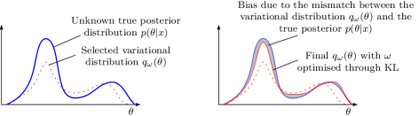
Figure 1: Optimisation process of finding the closest variational distribution $q_{\omega}(\theta)$ over the set of latent variables $\omega$.

4 Variational Bayes method in survival analysis

The use of the model of the form (7) with an ANN as $h_{\mathbf{z}}(\mathbf{x})$ results in the integral (9) that cannot be calculated analytically. Obtaining the posterior probability density function $p(\theta|x)$ thus requires an approximation. ANNs typically have hundreds of parameters, precluding even the use of Monte Carlo methods. Another option are Gaussian processes that are shown to be equivalent to a fully connected ANN with an infinite number of hidden units in each layer [57]. A variational inference approach provides a computationally efficient solution using ELBO (11) as the loss function.

With the VB method, one has to select the prior distribution $p(\theta)$ and the variational family of the posterior distribution $\mathcal{Q}$. This is followed by optimisation (10) using the ELBO loss function (11), resulting in the variational distribution latent parameters $\omega^{*}$. In the most general form of the VB method, every model parameter may be treated as a stochastic one.

We implement the function $h_{\mathbf{z}}(\mathbf{x})$ as an ANN. The model parameters are assembled as $\theta=[\sigma,\mathbf{z}]$, $\mathbf{z}]=[\mu_{1},\ldots,\mu_{K}$. We use a mean-field variational family, so the probability distribution $q_{\omega}(\theta)$ can be expressed as

$$q_{\omega}(\theta)=q_{0}(\sigma)\cdot\prod_{k=1}^{K}q_{k}(z_{k}),$$ (12)

where $K$ is the number of the ANN parameters. For the variational distribution, we use a half-normal distribution for the factor $q_{0}(\sigma)$ and normal distribution for every $q_{k}(z_{k})$. The vector of latent parameters $\omega$ is structured as $\omega=[\sigma_{\sigma},\omega_{\mathbf{z}}]$, $\omega_{\mathbf{z}}=[\mu_{1},\ldots,\mu_{K},\sigma_{1},\ldots,\sigma_{K}]$. The latent parameter $\sigma_{\sigma}$ is used in $q_{0}(\sigma)=\frac{2}{\sigma_{\sigma}}\phi\left(\frac{\sigma}{\sigma_{\sigma}}\right)$ for $\sigma\geq 0$ and the latent parameters $\omega_{\mathbf{z}}$ define $q_{k}(z_{k})=\frac{1}{\sigma_{k}}\phi\left(\frac{z_{k}-\mu_{k}}{\sigma_{k}}\right)$, where $\phi$ is the probability density function of the standard normal probability distribution.

Models relying on the VB method are described using the concepts of probabilistic graphical models [58, 59] and directed factor graphs [60]. The model (7) is transformed into a VB form that takes censoring of the observations into account. The directed factor graph is shown in Figure 2.

Figure 2: Factor graph describing the devised survival model. The pseudocode of parameter estimation is shown in Algorithm 1. The expression 1-CDF_W is the predicted survival function and Bernoulli denotes the Bernoulli distribution. The latent variable $\omega_{k}$ stands for $\omega_{k}=[\mu_{k},\sigma_{k}]$. The model predicts the time-to-event from the covariates and the probability of censoring for a given maximum time-to-event.

The used VB approach relies purely on numerical evaluation and requires only proper specification of the model. That is, only the model likelihood $p(x|\theta)$ and the observations for parameter estimation $x$ have to be specified. The prior probability distribution $p(\theta)$ is assumed to be constant and the variational family $\mathcal{Q}$ is chosen. In our case, the likelihood is given by equation (7) and the variational family $\mathcal{Q}$ is as described in equation (12).

4.1 Parameter estimation

As derived by Wingate and Weber [61], the gradient of the criterion function is expressed as

$$\nabla_{\omega}\mathcal{L}(\omega)=\mathbb{E}_{q_{\omega}(\theta)}\left[\nabla_{\omega}\log q_{\omega}(\theta)\left(\log p(x,\theta)-\log q_{\omega}(\theta)\right)\right],$$ (13)

where $\mathcal{L}(\omega)$ is ELBO. This expression is used in stochastic gradient optimisation to find an estimate of $\omega^{*}$.

The likelihood of the $i^{\text{th}}$ training data point for a sampled value of $\theta$ is calculated based on equation (7). As illustrated in Figure 2, the evaluation process depends on whether the observation is censored or not. The vector of covariates is labelled with $\mathbf{x}^{(i)}$, $y^{(i)}$ is the logarithm of the time-to-event or time-to-censoring, and $c^{(i)}$ is the censoring label. For a complete observation, i.e. $c^{(i)}=0$, the gradient (13) is calculated at the observed $y^{(i)}$. For censored observations, i.e. $c^{(i)}=1$, the loss is calculated from the predicted probability of censoring at $y^{(i)}$, which equals the survival function 1-CDF_W at $y^{(i)}$. That is, the predicted probability distribution of $c^{(i)}$ is Bernoulli with the expected value of 1-CDF_W. The complete procedure is also shown as pseudo code in Algorithm 1. For the initial guess $\omega^{(0)}$, we use $\sigma_{\sigma}=5$ and $\mu_{k}=0$, $\sigma_{k}=1\;\forall\;k\in\{1,\ldots,K\}$.

1:Input $N$ observations, $\mathbf{x}^{(i)}$ are covariates, $y^{(i)}$ is logarithm of time-to-event or time-to-censoring, and $c^{(i)}$ is censoring label, $i\in\{1,\ldots,N\}$. Variational family $\mathcal{Q}$, prior $p(\theta)$, model structure $p(y|\mathbf{x},\theta)$.

2:Output Vector of latent parameters $\omega$, approximating $\omega^{*}$, specifying the variational density $q_{\omega}(\theta)$

3:Initialize latent parameters $\omega^{(0)}\in\Omega$

4:Initialize rate parameter $\alpha$ $\triangleright$ Using ADAM optimiser, this is adaptable

5:while  not ELBO convergence  do

6:     draw $\sigma\sim q_{0}(\sigma)=\frac{2}{\sigma_{\sigma}}\phi\left(\frac{\sigma}{\sigma_{\sigma}}\right),\,\sigma\geq 0$ $\triangleright$ half-normal distribution

7:     for all $k\in\{1,\ldots,K\}$ do$\triangleright$ loop through parameters of the ANN

8:         draw $z_{k}\sim q_{k}(z_{k})=\mathcal{N}(\mu_{k},\sigma_{k}^{2})$ $\triangleright$ $\theta=[\sigma,\mathbf{z}]$

9:     end for

10:     for all $i\in\{1,\ldots,N\}$ do $\triangleright$ loop through observations

11:         if $c^{(i)}=0$  then $\triangleright$ non-censored observations

12:              $l^{(i)}=\log p(y^{(i)}|\mathbf{x}^{(i)},\theta)$ $\triangleright$ term in stochastic gradient

13:         else$\triangleright$ censored observations

14:              $\Pr[c^{(i)}|y^{(i)},\mathbf{x}^{(i)},\theta]=1-\int_{-\infty}^{y^{(i)}}p(y|\mathbf{x}^{(i)},\theta)\,dy$ $\triangleright$ probability of surviving beyond $y^{(i)}$

15:              $l^{(i)}=\log\Pr[c^{(i)}|y^{(i)},\mathbf{x}^{(i)},\theta]$ $\triangleright$ term in stochastic gradient

16:         end if

17:     end for

18:     Compute the gradient $\nabla_{\omega}\mathcal{L}(\omega)$ of equation (13) $\triangleright$ $\log p(x,\theta)=\sum_{i=1}^{N}l^{(i)}$, and $q_{\omega}(\theta)$ is known

19:     Update $\omega^{(j+1)}=\omega^{(j)}+\alpha\nabla_{\omega}\mathcal{L}(\omega)$

20:end while

Algorithm 1 VB-based model parameter estimation assuming normal distribution as the variational family.

4.2 Estimating the survival function $S(t)$

Solving the survival model in the Bayesian framework, the survival function $S(t|\mathbf{x})$ for a given value of the covariates $\mathbf{x}$ and of the model latent parameters $\omega$ can be obtained as the posterior prediction distribution using the identified variational distribution $q_{\omega}(\theta)$ instead of the true unknown posterior. The probability density function is

$$p_{\omega}(t|\mathbf{x})=\int p(t|\mathbf{x},\theta)q_{\omega}(\theta)\,d\theta.$$ (14)

The survival function $S(t|\mathbf{x})=\Pr[T\geq t]$ is by definition expressed as

$$S(t|\mathbf{x})=1-\int_{0}^{t}p_{\omega}(s|\mathbf{x})\,ds=1-\int_{0}^{t}\!\!\int p(s|\mathbf{x},\theta)q_{\omega}(\theta)\,d\theta\,ds$$ (15)

and can be evaluated from (15) using Monte Carlo integration. It is a fairly simple and computationally efficient process. The pseudo code is presented in Algorithm 2.

1:Input covariates $\mathbf{x}$, model structure $p(y|\mathbf{x},\theta)$, variational distribution $\mathcal{Q}$, latent parameters $\omega$, variational model $p_{\omega}(y|\mathbf{x})=\int p(y|\mathbf{x},\theta)q_{\omega}(\theta)\,d\theta$, number of samples $N_{\text{MCMC}}$

2:Output $S(t|\mathbf{x})=\Pr(y>\log t|\mathbf{x})=n(t)/N_{\text{MCMC}}$

3:for all $k\in\{1,\ldots,N_{\text{MCMC}}\}$ do$\triangleright$ Monte Carlo integration

4:     draw $\theta_{k}\sim q_{\omega}(\theta)$

5:     draw $y_{k}\sim p(y|\mathbf{x},\theta_{k})$

6:end for

7:$b_{k}(t)=\begin{cases}1,&\text{if }y_{k}>\log t\\ 0,&\text{otherwise}\end{cases}$

8:$n(t)=\sum_{k=1}^{N_{\text{MCMC}}}b_{k}(t)$

Algorithm 2 Prediction of survival function $S(t|\mathbf{x})$.

We have mentioned that Monte Carlo integration of the integral (9) would be too computationally intensive, but the integral (15) is easy to calculate using the Monte Carlo method even though the integration variable $\theta$ has the same dimensionality in both cases. The reason is that the probability density function $q_{\omega}(\theta)$ is quite different from $p(\theta)$. While $p(\theta)$ is very wide – we take it to be constant over $\Re^{+}\times\Re^{K}$ – and the integration would require a lot of samples, the function $q_{\omega}(\theta)$ is much more localized, so every sample contributes a lot more to the accuracy of the result and a much lower number is sufficient.

5 Variational Bayesian survival analysis applied to unemployment modelling

PES records provide a rich description of job seekers in the form of their profiles. One of the most common metrics that PES associates with every job seeker is the so-called probability of exit, referring to “exiting” from their records. It should be noted that not every “exit” is due to employment but also events such as retirement, PES determining that someone is not genuinely seeking a job, and many others.

Some of the job seekers entering the records at any point in time have exited at a later known date while the others are still unemployed. From the data perspective, this is a clear example of a right censored data. Survival analysis is therefore a viable tool for analysing PES data where the probability of exit from PES records serves the function of the hazard rate.

5.1 Data structure

Every job seeker is described using 19 covariates. Some describe personal characteristics of each job seeker such as age, gender, education based on the national classification, last work position based on ESCO classification, municipality of the permanent residence, country of origin, duration of work experience, date of entering the unemployment records, date of employment, and limitations such as disability. The others describe the interventions of the public employment service, for instance courses attended, employment plan, unemployment benefits, social security benefits and active job seeking grade. The covariates represent a mix of continuous and discrete variables with very different cardinality. The complete list of the discrete covariates and their cardinalities is shown in Table 2. It should be noted that the covariates with cardinality 2 are treated as continuous and do not go through the process of embedding.

Table 2: List of covariates and their cardinality

Continuous covariates	Discrete covariates (cardinality)
Day of PES entry	Specific profession category (109)
Month of PES entry	Profession program (2336)
Age	Municipality (215)
Months of work experience	Employment plan status (5)
eApplication	PES Office (61)
Gender	Reason for PES Entry (10)
Employment plan ready	Employability assessment (6)
Social benefits	Education category (22)
Unemployment benefits	Profession (ESCO) (3772)
	Disabilities (17)

5.2 Model error distribution

When defining the survival model, one of the key decisions is the selection of the probability density function of the error $W$ in (7). Since the probability of finding a job decreases over time [11], the suitable choices of $W$ are the ones that result in decreasing hazard rate $\lambda(t)$. The typical choices such as Gumbel or other extreme value distributions behave in the opposite way. For Gumbel probability density function of $W$, the resulting baseline survival time would follow the Weibull distribution and the hazard rate would rise over time. Such behaviour is reasonable in many uses of survival analysis but not in modelling of unemployment.

There are several possible choices of the probability density function of $W$ that result in a time-decreasing hazard rate. The simplest one is the normal distribution. For given values of $\mathbf{z}$ and $\mathbf{x}$, the survival time $T$ in (7) then follows the log-normal distribution and the hazard rate is monotonically decreasing after its maximum [44]. The probability density function of the event $f(t)$ in (1) and the corresponding survival function $S(t)$ become

$$\begin{split}f(t)&=\frac{\phi\left(\frac{\log t-\mu}{\sigma}\right)}{t}\quad\textrm{and}\\ S(t)&=1-\Phi\left(\frac{\log t-\mu}{\sigma}\right),\\ \end{split}$$ (16)

where $\phi$ and $\Phi$ are the probability density and the cumulative density functions of the standard normal distribution, respectively. Some typical shapes of the hazard functions for various values of $\mu$ and $\sigma$ are shown in Figure 3.

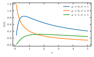
Figure 3: Various shapes of the hazard function $\lambda(t)$ for various parameters of the log-normal distribution.

5.3 Artificial neural network model for the risk function $h_{\mathbf{z}}(\mathbf{x})$

The underlying risk function $h_{\mathbf{z}}(\mathbf{x})$ is modelled using a deep ANN of the architecture shown in Figure 4. At the entry level of the network, the dimensions of categorical (discrete) covariates are reduced and the continuous covariates are normalised. The network then follows three repeating groups of linear layers, normalisation, and dropout [62]. The cardinality of the categorical covariates ranges from simple boolean (yes/no) up to 3772 categories for a covariate describing occupation. The dimensions are reduced using embedding [25] with the reduced number of dimensions equal to

$$n=\min\left(50,\left\lfloor\frac{d}{2}\right\rfloor+1\right),$$ (17)

where $d$ is the original number of categories.

Figure 4: ANN architecture for describing the risk function $h(\mathbf{x})$.

As listed in Table 2, there are 9 continuous covariates and 10 discrete ones. Using (17), the categorical values are embedded into 262 dimensions. Therefore, the first linear node has 271 input and 200 output values. The structure of the other layers is shown in Figure 4.

The variational distribution of each ANN parameter $z_{i}$ is the normal distribution $q_{\omega_{i}}(z_{i})$. The latent parameters $\omega_{i}=\{\mu_{i},\sigma_{i}\}$ represent the mean values and the variances of the variational distribution. In essence, such a choice means that the resulting variational distribution will not be able to capture any dependencies among the the network parameters. However, this is not a general limitation of the method. The mean-field approximation treats the latent parameters of the selected variational distribution as mutually independent [49]. The model parameters, in our case the weights of the neural network, would not have to be treated as mutually independent. The standard normal distribution is used for $W$, and the parameter $\sigma$ is sampled from a half-normal distribution.

6 Results

The data set contains daily updates on every job seeker in Slovenia from 2011 up to 2020. The network is trained on the data covering 12 months and evaluated on the records from the following 6 months. The presented results show the evaluation on the first 6 months of 2012 using a network trained on the set spanning the whole year of 2011. This is the most dynamic period in the labour market, a consequence of the global financial crisis. The training set, spanning from January 2011 until December 2011, contains 99,139 records. Of those, 55% have censored events, i.e. a potential exit from PES records occurred after the observation window. The evaluation set, spanning from January 2012 until July 2012, contains 43,641 records. It should be noted that exit from PES records can be due to various reasons, for instance employment, retirement, additional schooling, maternity leave, etc.

Figure 5 shows the identified survival curves of two typical job seekers plotted over a period of 1 year starting from the time of entry on the PES records. As expected, the survival probability $S(t)$ for a job seeker unemployed over the next 12 months remains high. Conversely, for the case of a person that was employed, the survival function drops significantly. The results on $S(t)$ at a given value of $t$ for the population can be analysed from two viewpoints: pure classification and assessment of the probability of exit.

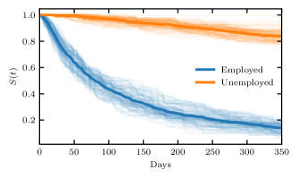
Figure 5: Typical shape of the modelled survival functions of the trained model. The pale lines are realisations of the $S(t)$ obtained from (14) by sampling the posterior distribution of the model parameters from (15) using Monte Carlo integration with 200 samples and each bold line is the average of 80 such realisations.

6.1 Hyperparameter selection

The optimisation is performed with the ADAM optimiser. We use two standard approaches for choosing the optimiser’s parameters. Initially, following the guidelines from Smith [63], the loss is checked over a range of optimiser’s parameters, in particular the learning rate. Furthermore, the impact of step wise adaptation of the learning rate is also checked as suggested in [64]. It should be noted that the whole data set is used in this analysis.

As shown in Figure 6, the minimal value of the loss function over a fixed number of iterations was achieved for learning rate somewhat above 1. Therefore, 1/10th of this learning rate is used for the training process.

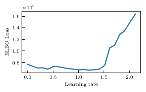
Figure 6: Values of ELBO loss after 4000 iterations for different values of the learning rate parameter.

6.2 Stopping criterion

Typically, the stopping criterion is a convergence of the ELBO loss (11), i.e., its relative change [65]. There are improved stopping criteria such as [66, 67], which use a combination of a smaller step size and Monte Carlo gradient estimates. The potential of such approaches becomes apparent for high dimensional problems.

In the case analysed here, it turns out that the decrease of the ELBO value is monotonic and converges to an asymptotic value after a certain number of iterations. This is shown in Figure 7. As a result, in this particular case the stopping criterion can be rather simple, i.e. using the heuristic approach that observes the relative change of the loss function values.

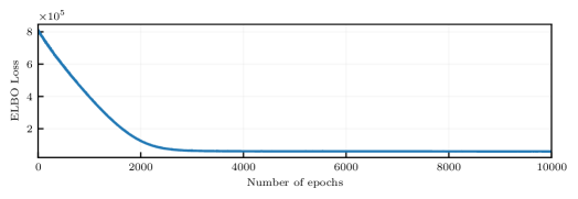
Figure 7: Evolution of the ELBO loss function over number of iterations.

6.3 Classification accuracy

Although the overall goal is not classification of the unemployed persons, viewing the results from a classification standpoint offers an easy way for quantifying the performance of the approach. A simple assessment of the model accuracy can be achieved by analysing the distribution of the survival probabilities of the whole test population at a certain time. In Figure 8, the values of the survival function $S(t)$ at $t=180$ days from entry are shown separately for the job seekers that exit the records in under 180 days and for the ones that stay unemployed longer. This value of $t=180$ days is chosen because more than 180 days of unemployment have a significant negative influence on a job seeker’s capability of finding a job [11]. Therefore, this result can be treated as an indicator of a job seeker’s capability of finding a job.

The classification accuracy depends on the selected threshold value. For threshold $S(t=180\,\text{days})=0.61$, the area under the ROC curve reaches the maximum. At this value, the classification accuracy is 75.6%, whereas the trivial model has 50.5% accuracy. The trivial model is the case when the whole test set is labelled as either employed or unemployed. The two groups are shown in Figure 8. The blue histogram contains persons that exited PES records prior to 180 days, which we label as positive outcome, and the orange histogram are persons that are either still on the records or exited after 180 days.

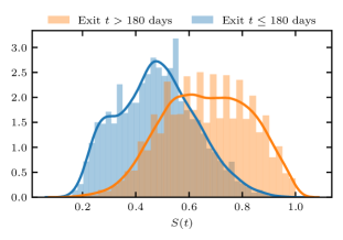
Figure 8: Distribution of the survival probability (remaining on the PES records) after 180 days for the test data for the period from January to June 2012. Training was on data from year 2011.

6.4 Survival analysis results

Unlike classification, the estimated survival probability over time $t$ offers a better insight. The set of job seekers remaining in the PES records for over 180 days is investigated into more detail. Table 3 lists the most common outcomes for these job seekers divided into three groups based by the values of $S(t=180\,\text{d})$. We are particularly interested in the ones for whom the model predicted survival probability below the threshold $S(t=180\,\text{d})<0.61$.

Table 3: Detailed overview of job seekers with exit time $T>180$ days based on the value of the survival function $S(t=180\,\text{d})$ and their outcome. The job seekers that exit the records through employment are divided further based on the time of event. The rest tend to end up being not active job seekers, meaning they quit fulfilling their obligations toward PES. Most of the remainder are employed by PES in public service, and a significant fraction of the rest go on maternity leave.

	$S(t=180\,\text{d})$ [%]
	<0.4	0.4–0.61	>0.61	Sum [%]
Employed, $T\leq 240$ days	1.2	6.0	2.5	9.8
Employed, $T>240$ days	1.6	13.7	20.0	35.3
Not active job seekers	1.5	10.1	25.0	36.6
Public service	0.1	1.6	6.2	8.0
Maternity leave	0.2	1.2	1.3	2.6
Other	1.5	2.3	4.0	7.7
Total	6.1	34.9	59.0	100.0

The false positives – the job seekers for whom the model assigns low survival probability $S(t=180\,\text{days})$ but remained for more than 180 days – deserve further attention as they may not get the necessary PES support if the model is relied upon. In Table 3, we split them into two subgroups based on $S(t=180\,\text{d})$ and compare them to the true negatives for whom the model correctly predicts over 180 days to exit. Let us term employment within a further 60 days, maternity leave, and having a less common outcome lumped as “other” a “good” outcome. An underestimate of the date of exit for under 60 days and the failure to take maternity leave into account are inconsequential for PES and hopefully for the job seeker. The “other” outcomes are of different desirabilities for the job seeker – they range from enrolling into further education up to imprisonment – but they tend to be independent of PES actions. Just like the people employed in 60 extra days and the ones on maternity leave, the “other” people are neither failed by PES nor a burden of PES. Therefore, assigning low survival probability to such a job seeker will not be likely to cause much harm.

The outcome is “good” for 30% of the false positives, rising to 47% with the model-predicted $S(t=180\,\text{d})<0.4$. In contrast, only 13.2% of the true negatives achieve a “good” outcome. It seems the type II error is more likely for the job seekers for whom it is less damaging, which is fortunate.

The fraction of the long-term job seekers of over 180 days that lose their status and become “not active” is the highest in the true negative $S(t=180\,\text{d})\geq 0.61$ group. For this group, losing the status is the most likely outcome. They lose the status by not fulfilling their obligations toward PES. It can be inferred that part of the group are the job seekers that PES actions did not help. Inexplicably from the data, the outcome is very common for job seekers around 60 years of age, indicating that there may be regulatory actions making the status less appealing to them. Detailed age profile results are shown in A.

The second most frequent outcome for the true negatives is getting employed after 240 days, thus using PES resources and suffering the consequences of unemployment for a longer time. A lot of the remainder get employed in public service, meaning that they stay in a contractual relationship with PES. The model-predicted $S(t=180\,\text{d})$ is strongly correlated with the probability of the job seeker serving in public service. This is not surprising as public service is only available to the long-term unemployed and there may be causal connections between the model inputs and the availability of public service to the job seeker.

7 Discussion on the accuracy

Two of the goals of PES are to get as many of the job seekers from their records employed as quickly as possible and to lower the number of long-term (over 1 year) unemployed [68]. The significance of long-term unemployment is that it has various negative consequences, some of which decrease the chance of getting employed [69, 11]. The presented model could help PES better estimate which job seekers need more assistance, potentially improving their service.

However, all of the reported accuracy results on implemented systems addressing unemployment records focus solely on classification. As a result, not many such systems became operational and others were disbanded due to fears of discrimination of the classification process. Most recently this happened with the Austrian AMAS system [70].

Due to the lack of proper profiling model results, the only comparable systems are those that perform classification. Even so, comparing the obtained 76% classification accuracy with the other published results has proven itself challenging. Due to data privacy regulations, it is not feasible to get access to data sets from various PES registries used in the literature. The algorithms are not published either, so it is not possible to apply them to the data that is available to us. Model comparison through applying different models to the same data is therefore not possible. We thus compare the reported results with the results of our model. One has to assume that the data sets of various PES organisations are of comparable quality and information content, and neglect the differences between labour markets in order to compare various modelling approaches this way.

Results of several systems implemented in PES offices are reported by Scoppetta and Buckenleib [71]. Table 4 shows a list of reported models comparable to the presented one, their underlying modelling methods and the resulting accuracies. In most published cases, the accuracy of the model in predicting the correct probability of exit over time is close to 70%.

Table 4: Summary of reported modelling results addressing the problems of unemployed persons profiling.

Reference	Method	Accuracy
Australia [72]	Logistic regression	Not reported
Austria [70]	Logistic regression	80-85%
Belgium [70]	Random forest	67%
Croatia [73]	Logistic regression	69%
Denmark [74, 75, 76]	Logistic regression	66%
Finland [6]	Statistical model	89%
France [12]	Logistic/Random forest/Neural networks	70%
Ireland [8]	Probit regression	69%
Netherlands [7]	Logistic regression	70%
New Zealand [77]	Random forest and Gradient boosting	63-83%

It should be noted that in many cases the reported accuracy listed in Table 4 refers to a particular subset of data, limited by gender, location, education, etc. Furthermore, there is no information on the balance of the test data, and it is easier to achieve a certain accuracy with a less balanced data set. The proposed VB model is tested on the whole population of job seekers, the data set is balanced (50.5% remained unemployed for longer than 180 days, and 49.5% was employed before that threshold), and the achieved accuracy is above the average reported in the literature. It can therefore be concluded that it works well. The source code is published and the curves of survival probability for each classification outcome are reported in Figure 8. It will thus be possible to compare the future models with the presented VB algorithm.

8 Conclusion

The study successfully introduces advanced survival analysis methods to the question of unemployment. It demonstrates the use of variational Bayesian methods for performing survival analysis with an arbitrary risk function implemented as an artificial neural network (ANN). The method enables a computationally efficient approximation of the posterior probability distributions. It thus becomes possible to exploit the true statistical nature of the survival analysis despite the need of using deep ANNs with a high number of parameters.

The proposed survival model predicts the time until exit from the job seeker records. As the most common reason of exiting the records is employment, the model provides time information regarding the probability of employment. This information is useful both for the job seekers and for the operation of the public employment service (PES). The model can assist the PES employment counsellors in recognising the job seekers that do not need PES resources as they will get employed soon regardless of the interventions. It thus enables the counsellors to focus their attention on the job seekers that need help.

Data analysis has been used to make predictions of similar kinds before. However, the performance of the proposed model cannot be accurately compared with the historical ones because the published results are incomplete. Based on the available data and the theoretical soundness, we believe that the proposed model performs relatively well.

The resulting model can be used for performing gamification scenarios allowing both the counsellors and the job seekers to explore various strategies for improving the job prospects, i.e. for reducing the survival probability. A limitation of the study is that it only explores the survival function and not the type of event that results in exiting the unemployment records. Most exits are of a desirable kind but some are not. Future research that includes the differences between types of exit and focuses on increasing the likelihood of desirable ones would be highly beneficial.

Ethics statement

The data for this analysis was provided by the public employment service in Slovenia in the framework of the EU H2020 HECAT project. All records were anonymised according to the General Data Protection Regulation of the European Union [78] and respecting all national privacy laws.

Appendix A Age distribution for inactive persons

The age distribution of unemployed persons that were identified as inactive by the PES office is shown in Figure 9. It is clear that the majority of the cases identified as not active job seekers are persons older than 50 years. There is no such significant skewness in the age distribution for persons with lower estimated survival probability.

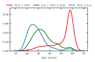
Figure 9: Age distribution of persons that were identified by PES counsellors as not active job seekers and remained on the PES records longer than 180 days. The age is taken at the moment of entry on the PES records. The plots represent kernel-density estimation of the observed number of records.

References

- Yizhong et al. [2017] X. Yizhong, Z. Lin, Y. Baranchenko, C. K. Lau, A. Yukhanaev, H. Lu, Employability and job search behavior: A six-wave longitudinal study of Chinese university graduates, Employee Relations 39 (2017) 223–239. doi:10.1108/ER-02-2016-0042.
- Arulampalam [2001] W. Arulampalam, Is unemployment really scarring? Effects of unemployment experiences on wages, The Economic Journal 111 (2001) F585–F606. URL: http://www.jstor.org/stable/798307.
- Virtanen et al. [2013] P. Virtanen, U. Janlert, A. Hammarström, Health status and health behaviour as predictors of the occurrence of unemployment and prolonged unemployment, Public Health 127 (2013) 46–52. URL: http://www.sciencedirect.com/science/article/pii/S0033350612003708. doi:10.1016/j.puhe.2012.10.016.
- Strandh et al. [2014] M. Strandh, A. Winefield, K. Nilsson, A. Hammarström, Unemployment and mental health scarring during the life course, European Journal of Public Health 24 (2014) 440–445. URL: https://academic.oup.com/eurpub/article-pdf/24/3/440/1290126/cku005.pdf. doi:10.1093/eurpub/cku005.
- Grundy [2015] J. Grundy, Statistical profiling of the unemployed, Studies in Political Economy 96 (2015) 47–68. doi:10.1080/19187033.2015.11674937.
- Riipinen [2011] T. Riipinen, Risk profiling of long-term unemployment in Finland, Dialogue Conference – Brussels, 2011. URL: http://ec.europa.eu/social/BlobServlet?docId=7583&langId=en.
- Wijnhoven and Havinga [2014] M. A. Wijnhoven, H. Havinga, The work profiler: A digital instrument for selection and diagnosis of the unemployed, Local Economy: The Journal of the Local Economy Policy Unit 29 (2014) 740–749. doi:10.1177/0269094214545045.
- O’Connell et al. [2009] P. J. O’Connell, S. McGuinness, E. Kelly, J. Walsh, National Profiling of the Unemployed in Ireland, number 10 in Resarch Series, Economic and Social Research Institute, 2009. URL: https://www.esri.ie/publications/national-profiling-of-the-unemployed-in-ireland.
- Loxha and Morgandi [2014] A. Loxha, M. Morgandi, Profiling the unemployed : A review of OECD experiences and implications for emerging economics, Technical Report, Social Protection and Labour No 1424, 2014. URL: http://hdl.handle.net/10986/20382.
- Sengul [2017] G. Sengul, Learning about match quality: Information flows and labor market outcomes, Labour Economics 46 (2017) 118–130. doi:10.1016/j.labeco.2017.04.001.
- Shimer [2012] R. Shimer, Reassessing the ins and outs of unemployment, Review of Economic Dynamics 15 (2012) 127–148. doi:10.1016/j.red.2012.02.001.
- Berthet and Bourgeois [2014] T. Berthet, C. Bourgeois, Towards ‘activation-friendly’ integration? Assessing the progress of activation policies in six European countries, International Journal of Social Welfare 23 (2014) S23–S39. doi:10.1111/ijsw.12088.
- Park et al. [2019] J. Park, I. B. Wood, E. Jing, A. Nematzadeh, S. Ghosh, M. D. Conover, Y.-Y. Ahn, Global labor flow network reveals the hierarchical organization and dynamics of geo-industrial clusters, Nature Communications 10 (2019) 3449. doi:10.1038/s41467-019-11380-w.
- López et al. [2015] E. López, O. Guerrero, R. L. Axtell, The network picture of labor flow (2015). arXiv:1507.00248.
- Anderson [1972] P. W. Anderson, More is different, Science 177 (1972) 393–396. doi:10.1126/science.177.4047.393.
- Kittel [2006] B. Kittel, A crazy methodology?: On the limits of macro-quantitative social science research, International Sociology 21 (2006) 647–677. doi:10.1177/0268580906067835.
- Erlinghagen [2019] M. Erlinghagen, Employment and its institutional contexts, KZfSS Kölner Zeitschrift für Soziologie und Sozialpsychologie 71 (2019) 221–246. doi:10.1007/s11577-019-00599-6.
- Huang et al. [2015] C.-Y. Huang, J. Ning, J. Qin, Semiparametric likelihood inference for left-truncated and right-censored data., Biostatistics 16 (2015) 785–798. doi:10.1093/biostatistics/kxv012.
- Robins [1995] J. M. Robins, An analytic method for randomized trials with informative censoring: Part 1., Lifetime data analysis 1 (1995) 241–254. doi:10.1007/BF00985759.
- Kittaneh and El-Beltagy [2017] O. A. Kittaneh, M. A. El-Beltagy, Efficiency estimation of type-I censored sample from the Weibull distribution based on sup-entropy, Communications in Statistics - Simulation and Computation 46 (2017) 2678–2688. doi:10.1080/03610918.2015.1056355.
- Ibrahim et al. [2001] J. G. Ibrahim, M.-H. Chen, D. Sinha, Bayesian Survival Analysis, Springer Series in Statistics, Springer New York, 2001. doi:10.1007/978-1-4757-3447-8.
- Cox [1972] D. R. Cox, Regression models and life-tables, Journal of the Royal Statistical Society: Series B (Methodological) 34 (1972) 187–202. URL: https://www.jstor.org/stable/2985181. doi:10.1111/j.2517-6161.1972.tb00899.x.
- Faraggi and Simon [1995] D. Faraggi, R. Simon, A neural network model for survival data, Statistics in Medicine 14 (1995) 73–82. doi:10.1002/sim.4780140108.
- Kovalev et al. [2020] M. S. Kovalev, L. V. Utkin, E. M. Kasimov, SurvLIME: A method for explaining machine learning survival models, Knowledge-Based Systems 203 (2020) 106164. URL: http://www.sciencedirect.com/science/article/pii/S0950705120304044. doi:10.1016/j.knosys.2020.106164.
- Guo and Berkhahn [2016] C. Guo, F. Berkhahn, Entity embeddings of categorical variables (2016). arXiv:1604.06737v1.
- Kvamme et al. [2019] H. Kvamme, Ø. Borga, I. Scheel, Time-to-event prediction with neural networks and Cox regression, Journal of Machine Learning Research 20 (2019) 1–30. URL: http://jmlr.org/papers/v20/18-424.html. arXiv:1907.00825.
- Katzman et al. [2018] J. L. Katzman, U. Shaham, A. Cloninger, J. Bates, T. Jiang, Y. Kluger, DeepSurv: personalized treatment recommender system using a Cox proportional hazards deep neural network, BMC Medical Research Methodology 18 (2018) 24. doi:10.1186/s12874-018-0482-1.
- Lee et al. [2020] C. Lee, J. Yoon, M. v. d. Schaar, Dynamic-DeepHit: A deep learning approach for dynamic survival analysis with competing risks based on longitudinal data, IEEE Transactions on Biomedical Engineering 67 (2020) 122–133. doi:10.1109/TBME.2019.2909027.
- Ching et al. [2018] T. Ching, X. Zhu, L. X. Garmire, Cox-nnet: An artificial neural network method for prognosis prediction of high-throughput omics data, PLOS Computational Biology 14 (2018) 1–18. URL: https://doi.org/10.1371/journal.pcbi.1006076. doi:10.1371/journal.pcbi.1006076.
- Giunchiglia et al. [2018] E. Giunchiglia, A. Nemchenko, M. van der Schaar, RNN-SURV: A deep recurrent model for survival analysis, in: Artificial Neural Networks and Machine Learning – ICANN 2018, Springer International Publishing, 2018, pp. 23–32. doi:10.1007/978-3-030-01424-7_3.
- Martinsson [2016] E. Martinsson, WTTE-RNN : Weibull Time To Event Recurrent Neural Network, Master’s thesis, Chalmers University Of Technology, 2016. URL: http://publications.lib.chalmers.se/records/fulltext/253611/253611.pdf.
- Šmídl and Quinn [2006] V. Šmídl, A. Quinn, The Variational Bayes Method in Signal Processing, Springer-Verlag, Berlin, Heidelberg, 2006. doi:10.1007/3-540-28820-1.
- Bui et al. [2017] T. D. Bui, J. Yan, R. E. Turner, A unifying framework for Gaussian process pseudo-point approximations using power expectation propagation, Journal of Machine Learning Research 18 (2017) 1–72. URL: http://jmlr.org/papers/v18/16-603.html. arXiv:1605.07066v3.
- Hensman et al. [2014] J. Hensman, A. Matthews, Z. Ghahramani, Scalable variational Gaussian process classification (2014). arXiv:1411.2005v1.
- Rezende et al. [2014] D. J. Rezende, S. Mohamed, D. Wierstra, Stochastic backpropagation and approximate inference in deep generative models, in: E. P. Xing, T. Jebara (Eds.), Proceedings of the 31st International Conference on Machine Learning, volume 32 of Proceedings of Machine Learning Research, PMLR, Bejing, China, 2014, pp. 1278–1286. URL: http://proceedings.mlr.press/v32/rezende14.html. arXiv:1401.4082v3.
- Yang et al. [2013] Z. Yang, L. Xie, C. Zhang, Variational bayesian algorithm for quantized compressed sensing, IEEE Transactions on Signal Processing 61 (2013) 2815–2824. doi:10.1109/tsp.2013.2256901.
- Oikonomou et al. [2019] V. P. Oikonomou, S. Nikolopoulos, I. Kompatsiaris, A novel compressive sensing scheme under the variational bayesian framework, in: 2019 27th European Signal Processing Conference (EUSIPCO), IEEE, 2019. doi:10.23919/eusipco.2019.8902704.
- Gruhl and Sick [2016] C. Gruhl, B. Sick, Variational bayesian inference for hidden markov models with multivariate Gaussian output distributions (2016). arXiv:1605.08618v1.
- Panousis et al. [2020] K. P. Panousis, S. Chatzis, S. Theodoridis, Variational conditional-dependence hidden markov models for human action recognition (2020). arXiv:2002.05809v1.
- Levine [2018] S. Levine, Reinforcement learning and control as probabilistic inference: Tutorial and review (2018). arXiv:1805.00909v3.
- Pivovarov et al. [2014] R. Pivovarov, D. J. Albers, J. L. Sepulveda, N. Elhadad, Identifying and mitigating biases in EHR laboratory tests, Journal of Biomedical Informatics 51 (2014) 24–34. doi:10.1016/j.jbi.2014.03.016.
- Pölsterl et al. [2016] S. Pölsterl, S. Conjeti, N. Navab, A. Katouzian, Survival analysis for high-dimensional, heterogeneous medical data: Exploring feature extraction as an alternative to feature selection, Artificial Intelligence in Medicine 72 (2016) 1–11. doi:10.1016/j.artmed.2016.07.004.
- Shafiq et al. [2017] M. Shafiq, M. Atif, R. Viertl, Generalized likelihood ratio test and Cox’s F-test based on fuzzy lifetime data, International Journal of Intelligent Systems 32 (2017) 3–16. doi:10.1002/int.21825.
- Klein and Moeschberger [2003] J. P. Klein, M. L. Moeschberger, Survival Analysis: Techniques for Censored and Truncated Data, Springer, New York, 2003. doi:10.1007/b97377.
- Tutz and Schmid [2016] G. Tutz, M. Schmid, Modeling Discrete Time-to-Event Data, Springer International Publishing, 2016. doi:10.1007/978-3-319-28158-2.
- Kaplan and Meier [1958] E. L. Kaplan, P. Meier, Nonparametric estimation from incomplete observations, Journal of the American Statistical Association 53 (1958) 457–481. doi:10.2307/2281868.
- Xiang et al. [2000] A. Xiang, P. Lapuerta, A. Ryutov, J. Buckley, S. Azen, Comparison of the performance of neural network methods and Cox regression for censored survival data, Computational Statistics & Data Analysis 34 (2000) 243–257. doi:10.1016/S0167-9473(99)00098-5.
- Ranganath et al. [2016] R. Ranganath, A. Perotte, N. Elhadad, D. Blei, Deep survival analysis, volume 56 of Proceedings of Machine Learning Research, PMLR, Northeastern University, Boston, MA, USA, 2016, pp. 101–114. URL: http://proceedings.mlr.press/v56/Ranganath16.html.
- Blei et al. [2017] D. M. Blei, A. Kucukelbir, J. D. McAuliffe, Variational inference: A review for statisticians, Journal of the American Statistical Association 112 (2017) 859–877. doi:10.1080/01621459.2017.1285773.
- Hoffman et al. [2013] M. D. Hoffman, D. M. Blei, C. Wang, J. Paisley, Stochastic variational inference, The Journal of Machine Learning Research 14 (2013) 1303–1347.
- Ranganath et al. [2013] R. Ranganath, S. Gerrish, D. M. Blei, Black box variational inference, 2013. arXiv:1401.0118.
- Kucukelbir et al. [2016] A. Kucukelbir, D. Tran, R. Ranganath, A. Gelman, D. M. Blei, Automatic differentiation variational inference, 2016. arXiv:1603.00788.
- Kingma and Ba [2014] D. P. Kingma, J. Ba, Adam: A method for stochastic optimization, in: 3rd International Conference for Learning Representations, May 7-9, 2015, San Diego, 2014. arXiv:1412.6980v9.
- Reddi et al. [2018] S. J. Reddi, S. Kale, S. Kumar, On the convergence of Adam and beyond, in: International Conference on Learning Representations, 2018. URL: https://openreview.net/forum?id=ryQu7f-RZ. arXiv:1904.09237v1.
- Paszke et al. [2019] A. Paszke, S. Gross, F. Massa, A. Lerer, J. Bradbury, G. Chanan, T. Killeen, Z. Lin, N. Gimelshein, L. Antiga, A. Desmaison, A. Kopf, E. Yang, Z. DeVito, M. Raison, A. Tejani, S. Chilamkurthy, B. Steiner, L. Fang, J. Bai, S. Chintala, PyTorch: An imperative style, high-performance deep learning library, in: H. Wallach, H. Larochelle, A. Beygelzimer, F. d'Alché-Buc, E. Fox, R. Garnett (Eds.), Advances in Neural Information Processing Systems 32, Curran Associates, Inc., 2019, pp. 8024–8035. URL: http://papers.neurips.cc/paper/9015-pytorch-an-imperative-style-high-performance-deep-learning-library.pdf.
- Bingham et al. [2019] E. Bingham, J. P. Chen, M. Jankowiak, F. Obermeyer, N. Pradhan, T. Karaletsos, R. Singh, P. Szerlip, P. Horsfall, N. D. Goodman, Pyro: Deep universal probabilistic programming, Journal of Machine Learning Research 20 (2019) 1–6. URL: https://jmlr.csail.mit.edu/papers/v20/18-403.html. arXiv:1810.09538.
- Lee et al. [2018] J. Lee, Y. Bahri, R. Novak, S. S. Schoenholz, J. Pennington, J. Sohl-Dickstein, Deep neural networks as Gaussian processes, in: Sixth International Conference on Learning Representations ICLR, 2018. URL: https://iclr.cc/Conferences/2018/Schedule?showEvent=161. arXiv:1711.00165.
- Bishop [2006] C. M. Bishop, Pattern Recognition and Machine Learning, Springer-Verlag, New York, 2006.
- Koller and Friedman [2009] D. Koller, N. Friedman, Probabilistic graphical models: principles and techniques, MIT Press, 2009.
- Minka and Winn [2008] T. Minka, J. Winn, Gates: A Graphical Notation for Mixture Models, Technical Report MSR-TR-2008-185, 2008. URL: https://www.microsoft.com/en-us/research/publication/gates-a-graphical-notation-for-mixture-models/.
- Wingate and Weber [2013] D. Wingate, T. Weber, Automated variational inference in probabilistic programming, 2013. arXiv:1301.1299.
- Srivastava et al. [2014] N. Srivastava, G. Hinton, A. Krizhevsky, I. Sutskever, R. Salakhutdinov, Dropout: A simple way to prevent neural networks from overfitting, Journal of Machine Learning Research 15 (2014) 1929–1958. URL: http://jmlr.org/papers/v15/srivastava14a.html.
- Smith [2018] L. N. Smith, A disciplined approach to neural network hyper-parameters: Part 1 – learning rate, batch size, momentum, and weight decay, 2018. arXiv:1803.09820.
- Smith [2017] L. N. Smith, Cyclical learning rates for training neural networks, in: 2017 IEEE Winter Conference on Applications of Computer Vision (WACV), 2017, pp. 464–472. doi:10.1109/WACV.2017.58.
- Kucukelbir et al. [2015] A. Kucukelbir, R. Ranganath, A. Gelman, D. M. Blei, Automatic variational inference in stan, 2015. arXiv:1506.03431.
- Ranganath et al. [2014] R. Ranganath, S. Gerrish, D. Blei, Black Box Variational Inference, volume 33 of Proceedings of Machine Learning Research, PMLR, Reykjavik, Iceland, 2014, pp. 814–822. URL: http://proceedings.mlr.press/v33/ranganath14.html.
- Dhaka et al. [2020] A. K. Dhaka, A. Catalina, M. R. Andersen, M. Magnusson, J. H. Huggins, A. Vehtari, Robust, accurate stochastic optimization for variational inference, 2020. arXiv:2009.00666.
- pos [2020] Poslovni načrt za leto 2020 Zavoda Republike Slovenije za zaposlovanje, Zavod Republike Slovenije za zaposlovanje, Ljubljana, 2020. URL: https://www.ess.gov.si/_files/13037/Poslovni_nacrt_2020.pdf.
- ana [2015] Dolgotrajno brezposelne osebe, Zavod Republike Slovenije za zaposlovanje, Ljubljana, 2015. URL: https://www.ess.gov.si/_files/7100/Analiza_DBO.pdf.
- Desiere et al. [2019] S. Desiere, K. Langenbucher, L. Struyven, Statistical profiling in public employment services: an international comparison, in: OECD Social, Employment and Migration Working Papers, OECD Publishing, Paris, 2019. doi:10.1787/b5e5f16e-en.
- Scoppetta and Buckenleib [2018] A. Scoppetta, A. Buckenleib, Tackling long-term unemployment through risk profiling and outreach. A discussion paper from the employment thematic network, in: European Commission – ESF Transnational Cooperation. Technical Dossier no. 6, May 2018, Publications Office of the European Union, Luxembourg, 2018. URL: https://www.euro.centre.org/publications/detail/3166.
- Ponomareva and Sheen [2013] N. Ponomareva, J. Sheen, Australian labor market dynamics across the ages, Economic Modelling 35 (2013) 453–463. doi:10.1016/j.econmod.2013.07.038.
- Pojarski [2018] P. I. Pojarski, Implementation Completion and Results Report 8426-HR, Technical Report ICR00004446, The World Bank, 2018.
- Rosholm et al. [2004] M. Rosholm, M. Svarer, B. Hammer, A Danish profiling system (November 25, 2004). Univ. of Aarhus economics working paper No. 2004-13, in: Discussion paper series, Aarhus University Economics Department, 2004. doi:10.2139/ssrn.1147586.
- Madsen [2014] P. K. Madsen, Youth Unemployment and the Skills Mismatch in Denmark, Technical Report, European Parliament, Directorate General for Internal Policies, 2014. URL: https://core.ac.uk/download/pdf/60647777.pdf.
- Larsen and Jonsson [2011] A. Larsen, A. B. Jonsson, Employability profiling system – the Danish experience, Presentation at PES, 2011. URL: http://ec.europa.eu/social/BlobServlet?docId=7584&langId=en.
- Obben [2002] J. Obben, Towards a formal profiling model to foster active labour market policies in New Zealand, Discussion paper (Massey University. Department of Applied and International Economics) no. 02.07, Dept. of Applied and International Economics, Massey University, Palmerston North, N.Z., 2002. URL: http://citeseerx.ist.psu.edu/viewdoc/download?doi=10.1.1.195.2652&rep=rep1&type=pdf.
- Council of European Union [2016] Council of European Union, Regulation (EU) 2016/679 of the European Parliament and of the Council of 27 April 2016 on the protection of natural persons with regard to the processing of personal data and on the free movement of such data, and repealing Directive 95/46/EC (General Data Protection Regulation), 2016. URL: https://eur-lex.europa.eu/eli/reg/2016/679/oj.