COVID-19 spreading under containment actions

Abstract

We propose an epidemiological model that includes the mobility patterns of the individuals, in the spirit to those considered in Refs. [1, 2, 3]. We assume that people move around in a city of 120$\times$120 blocks with 300 inhabitants in each block. The mobility pattern is associated to a complex network in which nodes represent blocks while the links represent the traveling path of the individuals (see below). We implemented three confinement strategies in order to mitigate the disease spreading: 1) global confinement, 2) partial restriction to mobility, and 3) localized confinement. In the first case, it was observed that a global isolation policy prevents the massive outbreak of the disease. In the second case, a partial restriction to mobility could lead to a massive contagion if this was not complemented with sanitary measures such as the use of masks and social distancing. Finally, a local isolation policy was proposed, conditioned to the health status of each block. It was observed that this mitigation strategy was able to contain and even reduce the outbreak of the disease by intervening in specific regions of the city according to their level of contagion. It was also observed that this strategy is capable of controlling the epidemic in the case that a certain proportion of those infected are asymptomatic.

1 Introduction

In the absence of a vaccine, strategies based on non-pharmaceutical interventions were proposed to contain the COVID-19 pandemic. Social distancing policies, specifically mobility restrictions and lockdowns, among others were the more common ones. Such policies should be implemented for long periods (typically months) to avoid re-emergence of the epidemic once lifted. Therefore, quantitative research is still needed to assess the efficacy of non-pharmaceutical interventions and their timings.

Many works analyze real-time mobility data in order to relate the changes in the mobility patterns and the disease propagation. Ref. [4] reports a correlation between the mobility pattern and the reduction of new infections. Besides, they found that it takes two to three weeks to see results due to the incubation time of the disease. Also, Ref. [5] carries out a detailed study of the effects of containment measures during the first 50 days of the COVID-19 epidemic in China. These researchers found that traveling restrictions and social distancing measures (among others) were effective in the containment of the disease. Ref. [6] analyzes real mobility datasets in many US metropolitan areas. They found that a small minority of “super-spreaders” places are the responsible for the wide propagation of the infection.

The changes in the mobility patterns are a consequence of the implementation of different quarantines. Ref. [7] analyzes different quarantine types considering a complex SEIR scheme. They suggested an alternative type of quarantine to reduce the infection disease while allowing a socio-economic activity. In a similar way, Ref. [8] proposes a cyclic schedule of 4-days work and 10-days lockdown. Also, an improved version of this strategy can be found in Ref. [9]. The influence of human behaviors on infectious disease transmission [10], the effects of vaccination during a pandemic [11] and the role of the “super-spreaders” [12, 13] are many other complex scenarios analyzed in the literature. However, a compressive and quantitative comparison of the effectivenesses of different lockdown and their timing appears to be lacking.

In this work we consider the spread of a disease mimicking the COVID-19, assuming a spatio-temporal SEIR model of mobile agents. We simulated and compared different confinement strategies in order to mitigate the disease propagation. In Section 2 we describe the characteristics of the epidemiological model and the different mitigation strategies. Section 3 details the simulation procedure. Section 4 displays the results of our investigation, while Section 5 is dedicated to the discussion of the main results. The conclusions are drawn in Section 6.

2 The epidemiological model

There are three main ingredients in the description of the COVID-19 contagion and spatial spreading: the scenario where the process takes place (Section 2.1), the mobility patterns of the individuals (Section 2.2) and the epidemiological dynamics of the individuals (Section 2.3).

2.1 The stage

City

The simulation of the evolution of COVID-19 is performed in a schematic city in which the basic unit is the block. The city is represented by an homogeneous urban area of $120\times 120~{}$blocks placed in a square grid. The size of each block is $100\,$m$\times 100\,$m. The simulated grid corresponds to a big city, like Buenos Aires, Argentina. Each block hosts 300 people but this quantity may vary during the day (see next Section). The total population of the simulated city is $4.32\,$M similar to the Ciudad Autonoma de Buenos Aires’ population.

Network construction

The human mobility pattern between the blocks is accomplished by building a weighted and directed network. The nodes represent the blocks, while the links represent the human mobility from one block to another one. We consider two different links: short and long links.

Each node is linked with its first neighbors by a short link, as we illustrate in Fig. 1a. They represent the human mobility pattern between all neighboring blocks. Notice that these links generate a connected graph. As we will see later, this characteristic of the network will allow the disease to reach all parts of the city (as long as it is not locked during the epidemic).

On the other side, recent investigation on human mobility shows that the traveling lengths of the individuals follows a Levy distribution given by [14]

$$P(r)\propto(r+r_{0})^{-\beta}$$ (1)

where $P(r)$ stands for the probability that an individual reaches a distance $r$, and $r_{0}=100\,$m and $\beta=1.75$ correspond to empirical parameters.

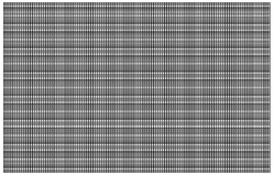
(a) Network with only short links

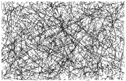
(b) Network with only long links

Figure 1: Schematic representation of a city network. The city is composed by $120~{}\times~{}120~{}$blocks placed on a square grid. They are linked by (a) four short links connecting neighboring nodes and (b) long links connecting far away nodes (see text for more details). The city corresponds to the union of these two sub-networks.

We built a network of long links following the Levy mobility pattern. This network is illustrated in Fig. 1b. The procedure was as follows

1. We randomly chose a node.

2. We then select randomly (according to the Levy distribution) the length $r$ of the next link.

3. We link the node from step 1 to any (random) node located at the distance $r$ in any direction.

Notice that each node may have more than one long link. Recall that these links are complementary to the short links connecting neighboring blocks (say, four neighbors per block).

The total number of long links will depend on how many times we repeat the above steps. Thus, we looped these steps until the geodesic path of the network resembled the one expected for a “small world” network [1]. As a general rule, we found that this condition was fulfilled after $25\%$ of the nodes had at least one long link. Table 1 summarizes the final set of parameter.

Finally, we stress the fact that the links between different blocks are assigned at the beginning of the simulation. Thereafter, the links remain fixed until the end of the simulation.

Table 1: Most relevant parameters used in the simulation of COVID-19 epidemic along the mobility network.

Number of nodes (blocks)	120$\times$120
Population per block	300
Short links	between first neighbors
Long links	over $25\%$ of the nodes
Total number of links	31825
$r_{0}$ (Levy distribution)	100 m
$\beta$ (Levy distribution)	1.75

2.2 Mobility pattern

We follow a similar scheme as in Ref. [1, 2] for the individuals’ mobility. This means that we divide the population of each block into two groups: stationary and non-stationary individuals. The former is composed by infected individuals while the latter is made up of susceptible, exposed and removed individuals.

We will assume that stationary individuals stay in their original block. We will further assume, in the spirit of Ref. [2], that $50\%$ of the non-stationary stay in their original block, while the other $50\%$ is considered to be mobile during the simulation. In this sense, we assume that $60\%$ of the non-stationary individuals travel (via short links) from their original block to the neighboring block. And, the remaining $40\%$ travel (via long links) from their original block to far blocks as indicated in Fig. 2.

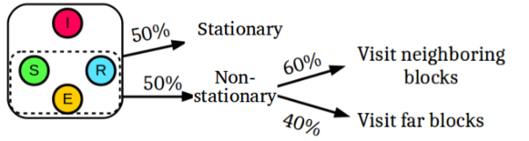
Figure 2: Schematic representation of the behavior of the population for a single block. The population is composed by susceptible (S), exposed (E), infected (I) and removed (R) individuals. Infected individuals stay at home during the simulation process while the $50\%$ of the susceptible, exposed and removed individuals move to another blocks (see text for more details).

Daily displacements of the individuals

Each moving individual is assumed to stay 1/2 of the day in its original block while the other 1/2 of the day he (she) moves to another block. They go to his (her) destination (work) everyday, and at the end of the day return back to their original block (home). This mechanism is performed reversing the direction of the links between blocks.

Fig. 3 shows a schematic representation of the human mobility pattern during each day (we illustrate this by a small city of 4$\times 4~{}$blocks for a better visualization). Recall from the last section that the links represent the mobility pattern between different blocks. Thus, moving humans travel through the links from one block to another one.

(a) Home (0-12 h)

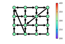
(b) Traveling to work

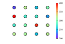
(c) Work (12-24 h)

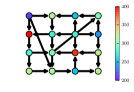
(d) Returning to home

Figure 3: (Color on-line only) Schematic illustration of the epidemic model incorporating individual human mobility during each day. The node colors represent the population of each block (see scale bar on the right). (a) The day starts with all individuals at home. (b) At 12 o’clock, $50\%$ of the population of each block moves to other cells, according to the pre-assigned mobility pattern. The arrows represent the movement direction. (c) The population of each block after mobile humans traveled to the working block. (d) Then, at 24 o’clock those humans that traveled from home to work return back to home. At the end of the day, the population of each block is the same as that in the beginning of the day. The sequence (a-d) repeats every day until the end of the simulation.

2.3 Epidemiological dynamics of the individuals

In order to describe the time evolution of a given population when a fraction gets infected, we resort to the SEIR compartmental models. These models consider that the individuals can be in four successive states: susceptible (S), exposed (E), infected (I) and removed (R). Details on each state can be found in Refs. [15, 16, 1, 2, 9]. The “exposed” state appears whenever the disease undergoes an “incubation” period, as occurs in the context of the COVID-19. The “removed” state includes either recovered and dead people.

The equations that describe the evolution of the infection read as follows [15, 16]

$$\left\{\begin{array}[]{ccc}\dot{s}(t)&=&-\beta i(t)s(t)\\ \dot{e}(t)&=&\beta i(t)s(t)-\sigma e(t)\\ \dot{i}(t)&=&\sigma e(t)-\gamma i(t)\\ \dot{r}(t)&=&\gamma i(t)\\ s(t)+e(t)+i(t)+r(t)&=&1\\ \end{array}\right.$$ (2)

where $s(t)=S(t)/N$, $e(t)=E(t)/N$, etc. correspond to the fraction of people in each state. For the purpose of simplicity, we will consider the coefficients $\beta$, $\sigma$ y $\gamma$ as fixed parameters. The parameter $\beta$ (infection rate) depends on intrinsic ingredients like the infectivity of the virus under consideration and extrinsic ones like the contact frequency. Besides, the parameters $\sigma$ and $\gamma$ depend exclusively on the illness under consideration.

The basic reproduction number $R_{0}$ is defined at the beginning of the propagation process as [17]

$$R_{0}=\frac{\beta}{\gamma}$$ (3)

This quantity represents the number of individuals that are infected by the first infected individuals (say, at the beginning of the disease). It is straight forward that the infection will blossom if $R_{0}$ is larger than 1. On the contrary, if this quantity is smaller than 1 the infection vanishes.

Fig. 4 shows the time evolution of either the SEIR model for a single block and for the whole mobility model (see caption for details). Notice that the latter shifts the date for the maximum infection to approximately 150. We will analyze this behavior in more detail in Section 4.

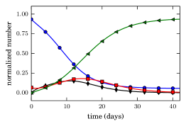
(a) basic SEIR model

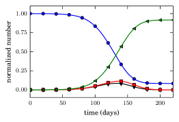
(b) spatio-temporal SEIR model

Figure 4: Normalized number of susceptibles ( ), exposed ( ), infected ( ) and removed ( ) as a function of time. In (a) we simulated a single block, while in (b) the scenario corresponds to a city composed by $120~{}\times~{}120~{}$blocks placed on a square grid (see Section 2.1). The plots are normalized with respect to the total population in the city: (a) 300 and (b) $4.32\,$M (i.e. 300 individuals per block). In both cases, the disease spreads without any kind of intervention strategy. The infection rate equals $\beta_{0}=0.75$ all along the propagation process. The simulation started with 20 infected individuals located in the single block (a) and at the central block of the city (b). The rest of the individuals were assumed to be in the susceptible state.

2.4 Lockdown types

In this section we define the proposed containment strategies which we have found useful in order to mitigate the disease. We divide the different types of quarantine according to their level of real life implementation difficulty

• Global lockdown

• Imperfect lockdown

• Local lockdown

Global lockdown scenario (GLs)

This type of lockdown consists in the isolation of each block. This means that people remain in their “home” blocks. We stress the fact that, within this strategy, society as a whole enters in lockdown. We illustrate this containment action in Fig. 5b.

Imperfect lockdown scenario (IGLs)

As in the previous case, the whole society adopts the same behavior. But, in this mitigation strategy, we partially reduce the movement between different blocks. Recall from Section 2.2 that $50\%$ of the non-stationary individuals move from their original block to another one. In this strategy, we reduce the level of mobility between blocks. Notice that the global quarantine corresponds to a full reduction of the mobility. We scheme this containment action in Fig. 5c.

Local lockdown scenario (LLs)

Unlike the other lockdown types, this applies to certain blocks and not to the whole society. Only those blocks that have a certain number of infected people are isolated. In this sense, the population of the isolated block are prohibited to travel around the city. This is achieved in practice by “cutting” the links to/from the infected blocks. We illustrate this containment action in Fig. 5d.

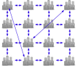
(a) Without lockdown

(b) Global lockdown

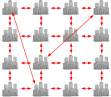
(c) Imperfect lockdown

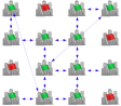
(d) Local lockdown

Figure 5: (a-d) Schematic representation of different types of mitigation strategies (exemplified by a $4\times 4$ grid). The lines represent the human mobility pattern between blocks. (a) People are allowed to evolve freely, equivalent to a “continuous activity” scenario. That is, there is no intervention during the epidemic. (b-d) Before a given day, individuals move freely from one block to another according to the mobility pattern. After that, (b) all blocks are isolated, (c) the flow between blocks (represented by red arrows) is reduced but the mobility pattern is unaffected, (d) those blocks with a number of infected individuals greater than a certain threshold are isolated (labeled with a red flag). The other blocks remain linked to each other (labeled with a green flag). See text for more details.

3 Numerical simulations

We integrate the SEIR equations by means of the Runge Kutta 4th-order method. The chosen time step was 0.1 (days). The SEIR equations were updated twice a day (after the people left their homes and after they returned back (see Figs. 3a and 3c).

As mentioned in Section 2.3, the parameters $\sigma$ and $\gamma$ represent the incubation rate and the recuperation rate, respectively. Therefore, $\sigma^{-1}$ and $\gamma^{-1}$ correspond to the mean incubation time and the mean recovery time, respectively. According to preliminary estimations for COVID-19, we consider the following parameter values for the SEIR model: $\sigma^{-1}=3\,$days and $\gamma^{-1}=4\,$days [5, 18, 19, 20, 21].

Infected individuals remain at their “Home” until evolving into the removed state. Susceptible, exposed and removed individuals are able to move from one block to another. The simulation started with 20 infected individuals located at the central block of the city, while the rest of the individuals were assumed to be in the susceptible state.

According to preliminary estimations for COVID-19, the basic reproduction number $R_{0}$ is (approximately) 3 [5, 22, 23]. This means that the infection rate $\beta_{0}$ is 0.75 (considering $\gamma^{-1}=4\,$days). The implementation of complementary health policies (use of mask, social distancing policies, among others) tends to reduce the contact frequency, and, therefore, the infection rate ($\beta$). Thus, we will also examine situations accomplishing infection rates of a fraction of $\beta_{0}$.

4 Results

We will examine three major scenarios affecting the human mobility:

1. The (global) lockdown scenario assumes that people remain confined at home until the epidemic is almost over. See details in Section 4.1.
   

2. The scenario where the confinement recommendation is followed by a fraction of the city inhabitants. We assume that the traveling individuals move around according to the Levy pattern explained in Section 2. See further details on this scenario in Section 4.2.
   

3. Mobility is suppressed only for the inhabitants of “infected blocks”. That is, common life mobility is sustained between blocks where no symptoms of the disease appeared. See Section 4.3 for details.
   

This last scenario is the most cumbersome one since “non-symptomatic” does not actually mean “non-infected”. We will explicitly introduce a set of “non-symptomatic” individuals in this scenario, in order to understand possible flaws to confinement.

4.1 Global lockdown scenario (GLs)

The GLs means that people remain confined within the block where she (he) lives. It corresponds to a sudden break of the mobility around the city in the context of our model. We assume, however, that people may still get in contact within their own block.

In this case, we consider the mobility suppression as the only heath-care policy. Additional health-care recommendations for the every day living (say, masks, common rooms disinfections, etc.) are considered in A. We will come back to this issue at the end of this Section.

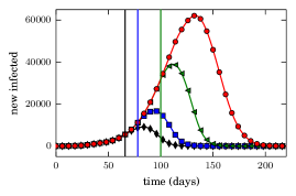
(a) Infected

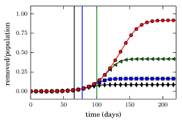
(b) Removed

Figure 6: (a) Number of new infected and (b) normalize number of removed as a function of time. The plot in (b) is normalized with respect to the total population in the city ($4.32\,$M). The GLs is applied when the number of new infected equals to:  5k, 10k and  30k new infected individuals. corresponds to the scenario of no lockdown at all. The infection rate remains constant along the simulation process and equals to $\beta_{0}=0.75$. That is, there is no complementary health-care policies during the lockdown. The different lockdown implementation days are indicated by vertical lines.

Fig. 6a shows the number of new infected people along time for three different lockdown periods (see caption for details). It is also shown the evolution for the case of no lockdown at all. The mobility cutoff prevents the infection curves in Fig. 6a from growing almost immediately after the beginning of the lockdown. The disease, however, disappears (approximately) 50 days (or 7 weeks) after. This is the time it take the susceptible or exposed individuals in each block to surpass the disease.

Fig. 6b exhibits the number of removed individuals as a function of time (see caption for details). These correspond to those individuals that previously appear as infected in Fig. 6a. It can be seen that the number of removed individuals increases since the outbreak of the disease, but it reaches a plateau soon after the lockdown is established. The plateau level, however, depends strongly on the starting date of the lockdown. Recall that the disease evolves only within the infected blocks after the lockdown implementation. Thus, the earlier the lockdown, the less number of infected (and removed) blocks at the end of the disease.

We now turn to the city map, in order to get a more accurate picture of the results so far. Fig. 7 displays the city as a square arrangement of blocks (see caption for details). Each “pixel” corresponds to a block, and the pixel color is associated to the corresponding scale on the left, which states the number of infected and the normalized number of removed per block. The snapshots capture the disease propagation from a single block located at the center of the map. A complete lockdown occurs at day 100.

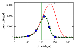
(a) Infected

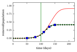
(b) Removed

Infected
Removed
Day 50	Day 80	Day 110	Day 130	Day 150

Figure 7: (a) Total number of new infected and (b) normalized number of removed as a function of time. The plot in (b) is normalized with respect to the total population in the city ($4.32\,$M). The GLs started at the day 100 after the first infected was detected. This is indicated by a vertical line in (a) and (b). The red continuous line corresponds to the scenario of no lockdown at all, while the lockdown case is indicated by green triangles. (Lower) Spatial distribution of the number of infected individuals for the five different dates (indicated in (a) and (b) by blue squares). The scale bar on the right corresponds to the number of infected and the normalized number of removed per block, respectively. The normalization was computed with respect to the population of each block. The infection rate remains constant along the simulation process and equals $\beta_{0}=0.75$. The city was composed by $120\times 120~{}$blocks placed on a square grid with 300 individuals per block.

The successive snapshots display a seemingly symmetrical propagation pattern, shortly after the outbreak. However, “secondary” focuses appear around the main focus due to those long traveling individuals. Recall that we assumed that human mobility follows a Levy-flight distribution (see Section 2).

Notice that the lockdown implementation (from day 100 onwards) somehow “freezes” the picture until the disease disappears (say, 50 days after). People continue to get infected within each block during the “quaratine” period. Complementary health-care recommendations may be required for the disease control within each block.

Fig. 8 shows the number of “infected blocks”, regardless of the number of infected people in the block (see caption for details). These curves quantify the infection map displayed in Fig. 7, and resumes the effects of the full lockdown.

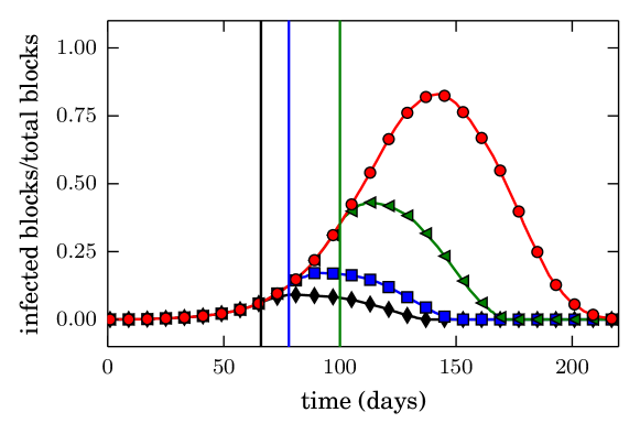
Figure 8: Normalized number of infected blocks as a function of time. The plot is normalized with respect to the total number of blocks ($14.4\,$k). Any block is classified as “infected” if at least one individual in the block is infected. We only consider people “living in the block” (say, those that sleep in there). The global lockdown is applied when the number of new infected equals to:  5k, 10k and 30k new infected individuals. corresponds to the scenario of no lockdown at all. The infection rate remains constant along the simulation process and equals $\beta_{0}=0.75$. That is, there is no complementary health-care policies during the lockdown. The different lockdown implementation days are indicated by vertical lines.

We may conclude that the GLs appears as a reliable strategy for avoiding the disease propagation. But the main drawback is that “non-infected” blocks will enter the “quarantine”. A further shows the effects of complementary health-care policies.

4.2 The imperfect global scenario (IGLs)

In this case we model a situation in which the GLs cannot be implemented. We distinguish, however, two groups which cannot be kept confined: workers from essential activities (say, health care, food supply or public order services, etc.) or those who decide not to accept the confinement recommendation. The former are expected to follow complementary health-care recommendations, while the latter might not. For this reason, we will examine relaxed confinement conditions and infection rates reduction.

Fig. 9a shows how the infection curves change as the number of agents which do not accept the movement restriction increases (see caption for details). The confinement starts at the vertical line. Notice that the propagation stops dramatically for the complete confinement situation. But the possibility of stopping the outbreak vanishes if a fraction of people (as small as $20\%$) still move around. A quick inspection of Fig. 9b confirms this point.

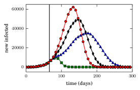
(a) Infected

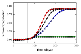
(b) Removed

Figure 9: (a) Number of new infected people and (b) normalized number of removed individuals as a function of time. The plot in (b) is normalized with respect to the total population in the city ($4.32\,$M). The IGLs is applied when the number of new infected equals to 5k (say, at day 66). From the lockdown implementation day, the percentage of individuals that move around is: $0\%$, $20\%$ and $50\%$. corresponds to the scenario of no lockdown at all ($100\%$ of moving people). We consider a partial break of the mobility as the only heath-care policy. Thus, the infection rate equals $\beta_{0}=0.75$ all along the propagation process.

We also notice from Fig. 9b that the total number of removed people at the end of the lockdown is the same for any IGLs. This appears to be in disagreement with the stochastic point of view, where the mobility reduction yields to the reduction in the probability of meeting people. We should remark that the meeting probability is somehow included in the infection rate $\beta$ within the SEIR model. Thus, for a complete picture of the IGLs, it is necessary to explore different values of $\beta$, as described below.

Fig. 10 examines the number of removed individuals (i.e. agents that have undergone the complete cycle of the illness, and have either reached a healthy state or have died) at the end of the epidemic in terms of the complementary health-care policies. Two startup days for the lockdown are shown (see caption for details). We can see that the number of removed individuals experiences a dramatic change at $\beta/\beta_{0}\approx 0.5$ for the different moving people situations, regardless of the startup day of the lockdown. This confirms the necessity of proper policies when these situations are expected to occur.

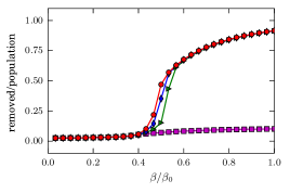
(a)

(b)

Figure 10: Normalized number of removed people as a function of the infection rate at the end of the epidemic. The plot is normalized with respect to the total population in the city ($4.32\,$M). The IGLs is applied when the number of new infected equals to: (a) 5k and (b) 30k. Since the lockdown implementation day, the percentage of individuals that move around is: $0\%$, $20\%$ and $50\%$. corresponds to the scenario of no lockdown at all ($100\%$ of moving people). Also, from the lockdown implementation day, the infection rate change from $\beta_{0}=0.75$ to $\beta$. The city was composed by $120\times 120~{}$blocks placed on a square grid with 300 individuals per block.

We improved on the above results by displaying in Fig. 11 the contour maps for different mobility situations, as a function of the lockdown date. Notice that Fig. 10 corresponds to date 66 in both contour maps (see caption in Fig. 10).

Fig. 11 expresses the fact that whenever the human mobility is suppressed, the number of removed individuals depends (almost exclusively) on the timing of the lockdown implementation. That is, the earlier the lockdown, the lower the number of removed. Besides, if mobility cannot be suppressed (say, $50\%$ of the people still move around), then complementary health-care policies should be heavily implemented, in order to avoid a massive contagion. This appears as an essential issue for late lockdowns.

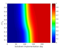
(a) $0\%$ of mobility

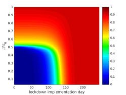
(b) $50\%$ of mobility

Figure 11: Normalized number of removed individuals (see scale on the right) as a function of the lockdown implementation day and the infection rate ($\beta/\beta_{0}$). The normalization was done taking into account the city population. The infection rate changes from $\beta_{0}=0.75$ to $\beta$ since the lockdown implementation day.

We close this section with the following conclusion: a complete mobility suppression appears as the most effective way of reducing the number of casualties. Essential workers following strict health-care recommendations (say, masks, behavioral protocols, etc.) that move around, however, will not spread the disease to uncontrolled levels. But, a small fraction of people moving around out of protocol can spoil the mitigation efforts.

4.3 Local lockdown scenario (LLs)

The local lockdown means that people remain confined within the block where he (she) lives, depending on the infection level of their block. That is, those blocks surpassing a certain “threshold” of infected people are immediately isolated, while the others remain “open”. As in the case of the GLs, we assume that people from an isolated block may still get in contact within this block. We consider the mobility break as the only heath policy.

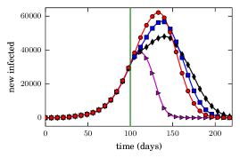
(a) Infected

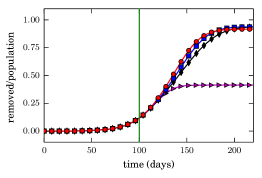
(b) Removed

Figure 12: (a) Number of new infected people and (b) normalized number of removed individuals as a function of time. The plot in (b) is normalized with respect to the total population in the city ($4.32\,$M). The LLs is applied when the number of new infected equals to 30k (indicate by the vertical line, at day 100). The locked blocks are those that exceed the following thresholds: 0, 5 and 10 individuals (see text for details). corresponds to the scenario of no lockdown at all. We consider the isolation of the infected blocks as the only heath-care policy. Thus, the infection rate equals $\beta_{0}=0.75$ all along the propagation process.

The local lockdown relies on the idea that the early detection of the infected can prevent the disease from spreading around the city. This idea presumes insignificant or null detection flaws. But in practice, a few infected individuals may not be detected due to wrong testings, or do not present symptoms at all. Our concern is on these situations. We will assume that a small fraction of infected people per block cannot actually be detected. This means that the lockdown occurs after surpassing a “threshold” of infected people (although not detected).

Fig. 12 represent the usual infection and passed over curves as a function of time, respectively (see caption for details). A quick inspection of these curves show that the disease decays almost immediately if the lockdown process occurs just after the first infected appeared in the block. Otherwise, the number of infected people continues increasing until the day 150 (approximately).

Fig. 12 can be compared to its counterpart in the context of the IGLs, that is, Fig. 9a. The time scales in both situations appear quite similar, although the curves in Fig. 12a do not extend further than 200 days.

(a) Infected threshold 0

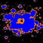
(b) Infected threshold 5

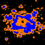
(c) Infected threshold 20

Figure 13: Spatial distribution of the blocks according to their infected state at the lockdown implementation day (100). Those blocks without infected individuals are represented in black, while those blocks with a number of infected people lower (greater) than the threshold (see legend) are represent in orange (blue). Blue blocks were isolated from the rest, while black and orange blocks were “opened”. The infection rate remains constant along the simulation process and equals $\beta_{0}=0.75$. The city was composed by $120\times 120~{}$blocks placed on a square grid with 300 individuals per block.

The “threshold” of non-detected people is responsible for the time lapse between the lockdown day and the end of the disease. This can be confirmed through Fig. 13, that shows the contour maps for the infected blocks (see caption for details). Notice that the non-detected blocks (say, the orange ones) become more relevant as the “threshold” level increases.

Fig. 14 exhibits the fraction of isolated blocks with respect to those blocks attaining at least an infected individual. We can observe that half of the infected blocks are actually not detectable for a threshold as low as 5 individuals per block. This is a strong warning on the effectivity of the LLs. Public health officers will lock down as many blocks as detected, but the undetected will actually continue the propagation.

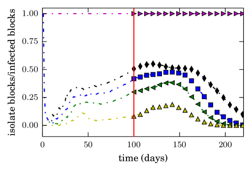
Figure 14: Normalized number of isolate blocks with respect to the total number of infected blocks as a function of time. The LLs is applied when the number of new infected equals to 30k (indicated by the vertical line, at day 100). The locked blocks are those that exceed the following thresholds: 0, 5, 10, 20 and 40 individuals (see text for details). The dashed lines corresponds to the behavior of both magnitudes before the lockdown implementation. The infection rate remains constant along the simulation process and equals $\beta_{0}=0.75$.

Whatever the efforts to detect infected, it seems that $40-45\%$ of the infected individuals do not experience noticeable symptoms [24]. We introduced this phenomenon into our simulations. Fig. 15 shows the overall removed people for an increasing number of “non-symptomatic” individuals. This confirms once more the lack of effectivity of the local lockdown if no other policy is established.

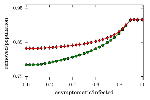
Figure 15: Normalized number of removed individuals (at the end of the epidemic) as a function of the percentage of asymptomatic individuals. The normalization was done taking into account the city population. The LLs started at the day 100 after the first infected was detected. The infection threshold is five individuals. From the lockdown implementation day, the infection rate switches from $\beta_{0}=0.75$ to $\beta=0.075$ in , while remains constant ($\beta_{0}$) in .

A thoughtful policy should include either strategic testings and backward tracing of the infected, from our point of view. We simulated this policy by tracing back any infected people to where she (he) belonged before being detected. The procedure in a nutshell is as follows:

• Test a random block. If infected, trace back all the individuals to the block they visited before.

• Test all the blocks recognized as visited immediately before.

• Lock down any of the above if infected.
  

The results from these simulations are shown in C. The testing procedure exhibits a noticeable efficiency (say, a noticeable decay in the number of removed people) if at least $80\%$ of the blocks can be tested. The back-tracing procedure further reduces this fraction significantly. Other complementary health-care policies (like masks, distancing, etc.) can also improve significantly the number of removed individuals (see C for details). In summary, the simulation results confirm our intuition on the effectivity of the back-tracing methodology.

We conclude from this Section that the effectivity of any LLs will strongly depend on breaking off the mobility of infected people. If this fails (because of asymptomatic or unreachable people), the disease will spread dramatically throughout the city. The strategic testing and back-tracing of the infected should be considered as an essential tool for the disease mitigation.

5 Analysis of the effects of the different strategies

In this Section we discuss the performance of the GLs, IGLs and LLs. We limit our analysis to the following points

• The performance of the lockdown is actually associated to the mitigation of the disease. Smooth infection curves are preferred in order to avoid stressing the medical care system.

• Lockdowns seriously damage the economy. The less disturbing and shorter lasting actions on non-infected people are therefore preferred.
  

We propose a merit function in order to rate the performance of the different lockdown strategies above mentioned, with respect to conditions (a) and (b). We will consider the fraction of the new infected people at any time $i(t)$ (or $i_{n}$ at step $n$ of the simulation) and the mobility $\mu(t)$ as the most relevant quantities for building the merit function (see below for the precise definitions). Thus, the merit function will be expressed as $C=C(i,\mu)$.

Notice from Section 4 that the maximum number of new infected people is quite different for the examined scenarios (see, for example, Figs. 9 and 12). Our merit function will consider the new infected people ($i$) normalized with respect to the maximum number of new infected when no lockdown is carried out. Accordingly, we will consider the mobility fraction ($\mu$) as the amount of traveling people normalized with respect to the traveling people before the lockdown.

The topic (a) concerns the infected people. The successful lockdown will mitigate the overall number of infected people. Our first proposal would be to rate the performance as the cumulative value of $i$ along the lockdown period. This approach, however, does not consider the stressing of the medical care system. For instance, it does not make any difference between sharp infection curves and smooth ones, provided that the total number of infected people are the same. We can therefore improve the proposed function by cumulating the fractions $i^{\alpha}$, for $\alpha>1$. The coefficient $\alpha$ introduces a penalty to the sharp maximum (see below).

The topic (b) concerns the non-infected people. The lockdown breaks the routine of the traveling fraction of people $\mu\,(1-i)$, and consequently, the economic activity. We propose rating the performance of the non-infected motion as the aggregate of a linear function of $\mu\,(1-i)$.

We express our merit function as follows

$$C=\displaystyle\sum_{n=1}^{N}\bigg{[}\overbrace{i_{n}^{\alpha}}^{\mathrm{(a)}}+\overbrace{A+B\,\mu_{n}\cdot(1-i_{n})}^{\mathrm{(b)}}\bigg{]}$$ (4)

where $n=1...N$ stands for the day of the lockdown. The term (a) refers to the medical care cost, and the term (b) refers to the economical cost.

Notice that in regular working days $i=0$ and $\mu=1$. This yields a daily economical cost equal to $A+B$, according to (4). We rate this cost as the null cost ($C=0$) for practical reasons. Thus, we set $A+B=0$ to hold this condition. The cost function then reads

$$C=\displaystyle\sum_{n=1}^{N}\bigg{[}\overbrace{i_{n}^{\alpha}}^{\mathrm{(a)}}+\overbrace{A\,[1-\mu_{n}\cdot(1-i_{n})}^{\mathrm{(b)}}]\bigg{]}$$ (5)

This expression shows that an increase in the number of new infected people (although keeping $\mu=1$) yields an increase in the medical cost (a) and the economical cost (b). The implementation of a strict lockdown ($\mu\rightarrow 0$) further increases the economical cost (b) to its maximum value. The intermediate situations will be more or less costly according to the balance between the medical care cost (a) and the economical cost(b) in expression (5). The parameter $A$ is the decisive parameter in the balance between the medical care, and economical cost.

We stress that the proposed function (5) is limited to items (a) and (b), while other presumably important arguments could have been left aside for simplicity. We also fixed $\alpha=2$ for practical reasons, but we checked that $C$ behaves qualitatively the same for other values $\alpha>1$ (not shown).

The parameter $A$ is actually the only free parameter in our cost function. It stands as a weighting factor for the economical cost. We will discuss the behavior of $C$ for the lockdown strategies appearing in Section 4 while varying the values of $A$.

Let us first examine the medical care cost (a) and economical cost (b) separately. Fig. 16 plots these costs for the situations shown in Figs. 9 and 12, respectively (see caption for details). The varying parameter is different on each plot, that is, the horizontal axis corresponds to the mobility in Fig. 16a and to the threshold level in Fig. 16b. The horizontal scale in Fig. 16a runs from the most strict situation at the origin ($\mu=0$) to the normal moving situation ($\mu=1$). Analogously, the horizontal scale in Fig. 16b runs from the most early detection at the origin to a detection level of 10 individuals. We present, however, both plots together in order to visualize the behavior of the GLs, IGLs and LLs as the lockdown becomes more and more relaxed. Fig. 16 resumes, indeed, the costs as a function of the lockdown strictness.

We notice from Fig. 16 that the medical cost, although different, shows a quite similar behavior in the IGLs and the LLs (see green squares in there). The economical costs, however, differ from each other when the lockdowns are very strict. The mutual differences vanish for the relaxed situations, no matter if the lockdown is global or local.

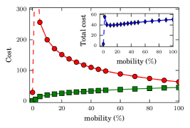
(a)

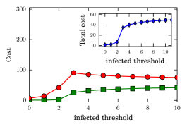
(b)

Figure 16: Medical care cost ( ) and economical cost ( ) for the scenarios analyzed in Section 4. The inset shows the total cost $C$ assuming $A=0.1$. (a) Implementation of the GLs and IGLs vs. $\mu$. The dashed lines means that the economical cost for mobilities between $0\%$ and $5\%$ are greater than 300. (b) Implementation of the LLs vs. the infection threshold. In both cases, the lockdown is applied when the number of new infected equals to 5k. The infection rate remains constant along the simulation process and equals $\beta_{0}=0.75$.

The dramatic increase of the economical cost (for the strict global lockdowns) is a matter of concern. Fig. 16a reports this phenomenon for small mobility values (IGLs), although not for the null mobility situation (GLs). The null mobility situation means that the disease remains confined to each block. But if a few agents avoid the lockdown, they can additionally spread the disease to other non-infected blocks. Thus, the perfect lockdown situation and the imperfect situation are quite different ones. This can be verified by observing Fig. 9. The infection curve smoothens and widens as the mobility switches from 0% to 20%. For a mobility fraction of 50% the curve narrows back again.

Either Fig. 9a and Fig. 16a point out that small mobility values induce a slow spreading dynamics (i.e. no massive propagation). This does not stress the medical care system, but yields long disruptions of the working routines. Notice from the cost expression (5) that the term (b) is linear to $N$ if $\mu\approx 0$. Thus, the long lasting lockdowns are responsible for the increase in the economical costs.

The LLs isolates the infected blocks only. The mobility is locally suppressed, and the whole scene undergoes a mixture of blocks with full mobility and blocks that are isolated. This is a dynamical process where the blocks become isolated and are opened back again. The net result is that the overall mobility is not significantly reduced along the lockdown, and therefore, the spreading dynamic does not “slow down” completely, as already noticed in Fig. 12a. Recall that the curves therein do not extend further than 200 days, no matter the detection threshold. This prevents the dramatic increase in the economic costs, as shown in Fig. 16b.

We turn now to the discussion of the different lockdown strategies performance. Fig. 17 shows the total cost $C$ as a function of the weighting factor $A$ (see caption for details). Notice that although $A$ can be chosen freely, it seems unrealistic to allow values yielding to costs beyond the cost of no-lockdown at all. We will consider the unlocked situation as the bounding value to $C$, as shown in red in Fig. 17 (see caption for details).

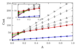
(a)

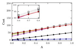
(b)

Figure 17: (a) Cost function $C$ as a function of the weighting parameter $A$ for the GLs and IGLs. From the lockdown implementation day, the percentage of individuals that move around is: $0\%$ (GLs), $5\%$, $10\%$, $25\%$ and $50\%$. (b) Cost function $C$ as a function of the weighting parameter $A$ for the LLs. The locked blocks are those that exceed the following thresholds: 0, 2, 3, 5 and 10 individuals. In both cases, corresponds to the scenario of no lockdown at all. Also, the lockdown is applied when the number of new infected equals to 5k. The infection rate remains constant along the simulation process and equals $\beta_{0}=0.75$.

Fig. 17 reports the minimum cost situation in blue color ( ) for the GLs and LLs. These correspond to either the most strict global lockdown ($\mu=0$) or the most early detection for the local lockdown (say, the null threshold). The latter attains a better performance with respect to the former for all the explored values of $A$.

The economical cost (b) is responsible for the slope of the curves in Fig. 17. The almost flat slope observed for the null threshold means that the daily cost for this situation is negligible. This is in agreement with an early detection, where the fraction of infected people is quite small ($i\approx 0$) and most of the non-infected people are allowed to move around ($\mu\approx 1$). The reader can check that this yields to vanishing values for the term (b) in our cost model (5).

We further notice that the curves’ slope increases for increasing detection thresholds in Fig. 17b. This occurs because of the increase in the daily economical cost, although the lockdown period remains close to $N\approx 200\,$days. Interestingly, the lockdown curves in Fig. 17b meet the no-lockdown curve for thresholds surpassing 2-3 infected people. This makes the lockdown curves only valid for small values of $A$ (say, below 0.7).

Recall that the IGLs experiences a dramatic increment of the economical cost for small mobility fractions (see Fig. 16a). As a result, the lockdown curves always meet the no-lockdown curve at some point (except for $\mu=0$), as shown in Fig. 17a. This is quite a difference with respect to the local strategy, since the lockdown curves are always limited to small values of $A$ (except for $\mu=0$).

Let us close the discussion with the following comments. We showed that the most strict implementation of either the global or local lockdown leads to the optimum performance (although the local one is preferred, as discussed above). But we noticed that there is some space left for partially effective lockdowns, if the most strict conditions are not attainable. The degree of effectiveness depends on the balance between the medical care costs and the economical costs, within this model.

6 Conclusions

This work concerns with the effect of human mobility in the context of a model for the spatio-temporal evolution of the COVID-19 outbreak. People move according to the Levy distribution and get into contact with each other during their daily routine. The lockdowns prevent these contacts from occurring, and thus, mitigate the propagation of the disease. Our investigation studies different lockdown scenarios and performs a careful evaluation of their effectiveness. We draw some recommendations for the better performance of the lockdown.

We assumed a SEIR compartmental model (with constant infection rates) for the inhabitants of a block. Each block was considered as a node within a square network of $120\times 120$ nodes. People were allowed to travel twice a day between blocks. The initial conditions for the simulations considered 20 infected individuals located at the central block of the network, while the rest of the individuals were assumed to be in the susceptible state.

We focused on three scenarios: the full lockdown of all the blocks (perfect scenario), the partial lockdown of all the blocks (imperfect scenario), and the lockdown of only the infected blocks (local lockdown). We sustained the lockdown until the disease propagation was (almost) over.

We first noticed that the success of any control action depends strongly on canceling the mobility around the city. But a small number of individuals may spoil the effectiveness of these actions if they do not follow the confinement recommendations. This is, in our opinion, the major risk when implementing any lockdown strategy.

We further built a cost function to rate the three strategies. We arrived to the conclusion that full lockdowns, or, the (very) early detection and isolation strategy are the most effective ones. The local isolation strategy is preferred, though, since it appears as the less costly in the context of our model.

It is important to emphasize that strict lockdown policies also allow for short periods of isolation. More relaxed lockdowns are less costly daily, but cumulate large costs after an extended period of time.

The full lockdown looses effectivenesses if the mobility is not completely canceled, as already mentioned. Our model shows that local lockdowns can still be quite effective even if a small number of infected people is not detected (and isolated). But the ultimate decision on whether to choose a global or local lockdown on a specific circumstance will depend on the right balance between the medical care cost and the economical cost due to routine disruptions. We will leave this discussion open to future research.

Appendix A Global lockdown with complementary health policies

We analyze here the effects of complementary health policies during the global lockdown. Fig. 18a shows the number of new infected people along time for three different infection rate (see caption for details). It is also shown the evolution for the case of no lockdown at all. The mobility cutoff prevents the infection curves in Fig. 18a from growing almost immediately after the beginning of the lockdown. In this sense, the more additional health policies, the faster decrease of the new infected individuals.

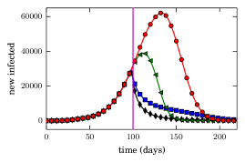
(a) Infected

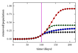
(b) Removed

Figure 18: (a) Number of new infected people and (b) normalized number of removed individuals as a function of time. The plot in (b) is normalized with respect to the total population of the city ($4.32\,$M). The global lockdown started at the day 100 after the first infected was detected. This is indicated by a vertical line in (a) and (b). Before this day, the infection rate equals to $\beta_{0}=0.75$. However, from this day, the infection rate equals: $(1/3)\beta_{0}$, $(1/2)\beta_{0}$ and  $\beta_{0}$. corresponds to the scenario of no lockdown at all. In the last case, the infection rate remains constant along the simulation process and equals to $\beta_{0}=0.75$.

Fig. 18b exhibits the number of individuals that passed over the disease as a function of time (see caption for details). These correspond to those individuals that previously appear as infected in Fig. 18a. First, it can be seen that the number of removed individuals increase since the outbreak of the disease. Second, it reaches a plateau soon after the lockdown is established. The plateau level, however, strongly depends on the complementary health policies. The more “intense” health policies (i.e. the lower infection rate), the lower number of removed individuals.

Appendix B Comparison between global and local lockdown

This appendix compare the global and local lockdown in terms of the new infected individuals. Recall that the global lockdown “cutoff” the human mobility around the city. In this sense, all blocks are isolated from the rest regardless of whether they are “infected” or not. On the contrary, the mobility is suppressed (depending the infected threshold) only for the inhabitants of “infected blocks” in the local lockdown.

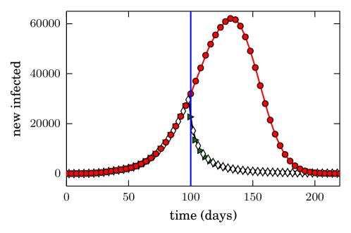
Figure 19: Comparison between the number new infected in the global ( ) and local ( ) lockdown scenario. The global and local lockdown started at the day 100 after the first infected was detected. This is indicated by a vertical line. From this day, all those infected blocks in which the number of infected exceeds 0 are isolated (in the local lockdown scenario). corresponds to the scenario of no lockdown at all. From the lockdown implementation day, the infection rate switches from $\beta_{0}=0.75$ to $(1/3)\beta_{0}$ (in both cases).

Fig. 19 shows the number of new infected people along time implementing a global and local lockdown (see caption for details). It is also shown the evolution for the case of no lockdown at all. It can be seen that both curves matches along time. This means that it is not necessary isolated all blocks to reduce the infection. In this sense, as can be expected, only is necessary isolated those infected blocks. Therefore, we can conclude that the local lockdown is the ”efficient” case of the global lockdown.

Appendix C Implementation of the testing $\&$ back-tracing strategy

We represent in this Section a possible testing procedure by means of a probability $p$ as follows:

1. We first chose (and test) a block at random with probability $p$.

2. If the chosen block is infected, we lock down the block until the disease disappears. If not, the block remains “open”.

3. We trace back and test all the individuals who visited the infected block.

4. We lock down any of the above blocks if infected.

5. We repeat this procedure every day.

Fig. 20 shows the number of new infected people along time for three different testing probabilities (see caption for details). It is also shown the time evolution for the case of no lockdown at all. Notice that the propagation decreases dramatically for the ideal tested scenario. But the possibility of stopping the outbreak vanishes in a bad (or poor) testing scenario. As can be seen in Fig. 20 the back-tracing of the infected improves the mitigation strategy.

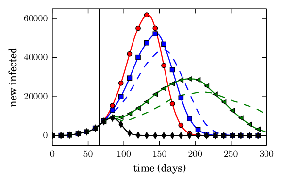
Figure 20: Number of new infected people as a function of time. The local lockdown is applied when the number of new infected equals to 5k (indicated by the vertical line). From the lockdown implementation day, we test each block with probability equal to:  $100\%$,  $75\%$ and $25\%$ (see text for details). corresponds to the scenario of no lockdown at all (i.e. $p=0\%$). Dashed lines corresponds to the scenario including back tracing of the infected individuals. Those infected blocks are isolated until the infection inside the corresponding block disappears. We consider the isolation of the infected blocks as the only heath policy. Thus, the infection rate equals to $\beta_{0}=0.75$ all along the propagation process.

Fig. 21 shows the number of removed individuals at the end of the epidemic in terms of the testing probability $p$ for three different complementary health policies (see caption for details). It can be seen that, in a scenario without complementary health policies (blue squares in Fig. 21), a massive testing (of more than $80\%$) is the only tool to avoid a wide spreading on the population. Note that this percentage is significantly reduced to $60\%$ if a back tracing policy is also implemented.

Notice from Fig. 21 that the implementation of strict complementary health policies (such as the use of a mask and social distancing) improves the mitigation of the disease.

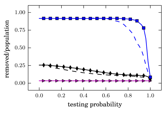
Figure 21: Normalized number of removed individuals at the end of the epidemic as a function of the testing probability. The normalization was done with respect to the city population. The local lockdown is applied when the number of new infected equals to 5k. From the lockdown implementation day, the infection rate switches from $\beta_{0}=0.75$ to:  $\beta_{0}$,  $(1/2)\beta_{0}$ and  $(1/3)\beta_{0}$ (see text for more details). Dashed lines corresponds to the scenario including back tracing of the infected individuals. Those infected blocks were isolated until the infection within the corresponding block disappears.

References

References

- [1] D. H. Barmak, C. O. Dorso, M. Otero, H. G. Solari, Dengue epidemics and human mobility, Phys. Rev. E 84 (2011) 011901.
- [2] D. Barmak, C. Dorso, M. Otero, Modelling dengue epidemic spreading with human mobility, Physica A: Statistical Mechanics and its Applications 447 (2016) 129 – 140.
- [3] A. D. Medus, C. O. Dorso, Diseases spreading through individual based models with realistic mobility patterns (2011). arXiv:1104.4913.
- [4] H. Badr, H. Du, M. Marshall, E. Dong, M. Squire, L. Gardner, Association between mobility patterns and covid-19 transmission in the usa: a mathematical modelling study, The Lancet Infectious Diseases 20 (11) (2020) 1247–1254.
- [5] H. Tian, Y. Liu, Y. Li, C.-H. Wu, B. Chen, M. U. G. Kraemer, B. Li, J. Cai, B. Xu, Q. Yang, B. Wang, P. Yang, Y. Cui, Y. Song, P. Zheng, Q. Wang, O. N. Bjornstad, R. Yang, B. T. Grenfell, O. G. Pybus, C. Dye, An investigation of transmission control measures during the first 50 days of the covid-19 epidemic in china, Science 368 (6491) (2020) 638–642.
- [6] S. Chang, E. Pierson, P. W. Koh, J. Gerardin, B. Redbird, D. Grusky, J. Leskovec, Mobility network models of covid-19 explain inequities and inform reopening, Nature 589 (2021) 82–87.
- [7] D. Meidan, N. Schulmann, R. Cohen, S. Haber, E. Yaniv, R. Sarid, B. Barzel, Alternating quarantine for sustainable epidemic mitigation, Nature Communications 12 (2021) 220.
- [8] O. Karin, Y. M. Bar-On, T. Milo, I. Katzir, A. Mayo, Y. Korem, B. Dudovich, E. Yashiv, A. J. Zehavi, N. Davidovich, R. Milo, U. Alon, Adaptive cyclic exit strategies from lockdown to suppress covid-19 and allow economic activity, medRxivdoi:10.1101/2020.04.04.20053579.
- [9] F. E. Cornes, G. A. Frank, C. O. Dorso, Cyclical lock-down and the economic activity along the pandemic of covid-19 (2020). arXiv:2006.06409.
- [10] S. Zhao, Y. Kuang, C.-H. Wu, K. Bi, D. Ben-Arieh, Risk perception and human behaviors in epidemics, IISE Transactions on Healthcare Systems Engineering 8 (4) (2018) 315–328.
- [11] A. D. Paltiel, J. L. Schwartz, A. Zheng, R. P. Walensky, Clinical outcomes of a covid-19 vaccine: Implementation over efficacy, Health Affairs 40 (1) (2021) 42–52.
- [12] E. Cave, Covid-19 super-spreaders: Definitional quandaries and implications, Asian Bioethics Review 12 (2) (2020) 235–242.
- [13] B. F. Nielsen, K. Sneppen, Superspreaders provide essential clues for mitigation of covid-19, medRxivdoi:10.1101/2020.09.15.20195008.
- [14] M. González, C. Hidalgo, A. Barabasi, Understanding individual human mobility patterns, Nature 453 (2008) 779–782.
- [15] R. M. Anderson, R. M. May, Infectious diseases of humans: dynamics and control, Oxford university press, 1992.
- [16] W. O. Kermack, A. G. McKendrick, A contribution to the mathematical theory of epidemics, Proceedings of the royal society of london. Series A, Containing papers of a mathematical and physical character 115 (772) (1927) 700–721.
- [17] S. W. Park, B. M. Bolker, D. Champredon, D. J. Earn, M. Li, J. S. Weitz, B. T. Grenfell, J. Dushoff, Reconciling early-outbreak estimates of the basic reproductive number and its uncertainty: framework and applications to the novel coronavirus (sars-cov-2) outbreak, medRxivdoi:10.1101/2020.01.30.20019877.
- [18] Y. M. Bar-On, A. Flamholz, R. Phillips, R. Milo, Science forum: Sars-cov-2 (covid-19) by the numbers, eLife 9 (2020) e57309.
- [19] https://www.who.int/es/health topics/coronavirus.
- [20] https://coronavirus.jhu.edu/.
- [21] The incubation period of coronavirus disease 2019 (covid-19) from publicly reported confirmed cases: Estimation and application, Annals of Internal Medicine 172 (9) (2020) 577–582.
- [22] E. C. for Disease Prevention, C. 2020, Coronavirus disease 2019 (covid-19) in the eu/eea and the uk - eighth update, Rapid Risk Assessment (8).
- [23] Y. Liu, A. A. Gayle, A. Wilder-Smith, J. Rocklöv, The reproductive number of COVID-19 is higher compared to SARS coronavirus, Journal of Travel Medicine 27 (2).
- [24] D. P. Oran, E. J. Topol, Prevalence of asymptomatic sars-cov-2 infection, Annals of Internal Medicine 173 (5) (2020) 362–367.