Variance Penalized On-Policy and Off-Policy Actor-Critic

Abstract

Reinforcement learning algorithms are typically geared towards optimizing the expected return of an agent. However, in many practical applications, low variance in the return is desired to ensure the reliability of an algorithm. In this paper, we propose on-policy and off-policy actor-critic algorithms that optimize a performance criterion involving both mean and variance in the return. Previous work uses the second moment of return to estimate the variance indirectly. Instead, we use a much simpler recently proposed direct variance estimator which updates the estimates incrementally using temporal difference methods. Using the variance-penalized criterion, we guarantee the convergence of our algorithm to locally optimal policies for finite state action Markov decision processes. We demonstrate the utility of our algorithm in tabular and continuous MuJoCo domains. Our approach not only performs on par with actor-critic and prior variance-penalization baselines in terms of expected return, but also generates trajectories which have lower variance in the return.

Introduction

Reinforcement learning (RL) agents learn to solve a task by optimizing the expected accumulated discounted rewards (return) in a conventional setting. However, in risk-sensitive applications like industrial automation, finance, medicine, or robotics, the standard objective of RL may not suffice, because it does not account for the variability induced by the return distribution. In this paper, we propose a technique that promotes learning of policies with less variability.

Variability in sequential decision-making problems can arise from two sources – the inherent stochasticity in the environment (transition and reward), and imperfect knowledge about the model. The former source of variability is addressed by the risk-sensitive Markov decision processes (MDPs) (Howard and Matheson 1972; Heger 1994; Borkar 2001, 2002), whereas the latter is covered by robust MDPs (Iyengar 2005; Nilim and El Ghaoui 2005). In this work, we address the former source of variability in an RL setup via mean-variance optimization. One could account for mean-variance tradeoffs via maximization of the mean subject to variance constraints (solved using constrained MDPs (Altman 1999)), maximization of the Sharpe ratio (Sharpe 1994), or incorporation of the variance as a penalty in the objective function (Filar, Kallenberg, and Lee 1989; White 1994). Here, we use a variance-penalized method to solve the optimization problem by adding a penalty term to the objective.

There are two ways to compute the variance in the return $\text{Var}(G)$. The indirect approach estimates $\text{Var}(G)$ using the Bellman equation for both the first moment (i.e. value function) and the second moment as $\text{Var}(G)=\operatorname{\mathbb{E}}[G^{2}]-\operatorname{\mathbb{E}}[G]^{2}$ (Sobel 1982). The direct approach forms a Bellman equation for the variance itself, as $\text{Var}(G)=\operatorname{\mathbb{E}}[(G-\operatorname{\mathbb{E}}[G])^{2}]$ (Sherstan et al. 2018), skipping the calculation of the second moment. Sherstan et al. (2018) empirically established that in the policy evaluation setting, the direct variance estimation approach is better behaved compared to the indirect approach, in several scenarios: (a) when the value estimates are noisy, (b) when eligibility traces are used in the value estimation, and (c) when the variance in return is estimated from off-policy samples. Due to the above benefits and the simplicity of the direct approach, we build upon the approach proposed by Sherstan et al. (2018) only for policy evaluation setting, and, develop actor-critic algorithms for both on- and off-policy settings (control).

Contributions: (1) We modify the standard policy gradient objective to include a direct variance estimator for learning policies that maximize the variance-penalized return. (2) We develop a multi-timescale actor-critic algorithm, by deriving the gradient of the variance estimator in both the on-policy and the off-policy case. (3) We prove convergence to locally optimal policies in the on-policy tabular setting. (4) We compare our proposed variance-penalized actor-critic (VPAC) algorithm with two baselines: actor-critic (AC) (Sutton et al. 2000; Konda and Tsitsiklis 2000), and an existing indirect variance penalized approach called variance-adjusted actor-critic (VAAC) (Tamar and Mannor 2013). We evaluate our on- and off-policy VPAC algorithms in both discrete and continuous domains. The empirical findings demonstrate that VPAC compares favorably to both baselines in terms of the mean return, but generates trajectories with significantly lower variance in the return.

Preliminaries

Notation

We consider an infinite-horizon discrete MDP $\langle\mathcal{S},\mathcal{A},\mathcal{R},P,\gamma\rangle$ with finite state space $\mathcal{S}$ and finite action space $\mathcal{A}$. $\mathcal{R}\in\operatorname{\mathbb{R}}$ denotes the reward function (with $R_{t+1}$ denoting the reward at time $t$). A policy $\pi:\mathcal{S}\rightarrow\mathcal{A}$ governs the behavior of the agent in state $s$, the agent chooses an action $a\sim\pi(\cdot|s)$, then transitions to next state $s^{\prime}$ according to transition probability $P(s^{\prime}|s,a)$. $\gamma\in[0,1]$ is the discount factor. Let $G_{t}=\sum_{l=0}^{\infty}\gamma^{l}R_{t+1+l}$ denote the accumulated discounted reward (also known as return) along a trajectory. The state value function for $\pi$ is defined as: $V_{\pi}(s)=\operatorname{\mathbb{E}}_{\pi}[G_{t}|S_{t}=s]$ and state-action value function is: $Q_{\pi}(s,a)=\operatorname{\mathbb{E}}_{\pi}[G_{t}|S_{t}=s,A_{t}=a]$. In this paper, $\operatorname{\mathbb{E}}_{\pi}[.]$ denotes expectation over transition function of MDP and probability distribution under $\pi$ policy.

Actor-Critic (AC)

The policy gradient (PG) method (Sutton et al. 2000) is a policy optimization algorithm that performs gradient ascent in the direction maximizing the expected return. Given a parameterized policy $\pi_{\theta}(a|s)$, where $\theta$ is the policy parameter, an initial state distribution $d_{0}$ and the discounted weighting of states $d_{\pi}(s)=\sum_{t=0}^{\infty}\gamma^{t}{P(S_{t}=s|s_{0}\sim d_{0},\pi)}$ encountered starting at some state $s_{0}$, the gradient of the objective function $J_{d_{0}}(\theta)=\sum_{s_{0}}d_{0}(s_{0})V_{\pi_{\theta}}(s_{0})$ (Sutton and Barto 2018) is given by:

$$\nabla_{\theta}J_{d_{0}}(\theta)=\operatorname{\mathbb{E}}_{s_{0}\sim d_{0}}\Big{[}\sum_{s}d_{\pi}(s)\sum_{a}\nabla_{\theta}\pi_{\theta}(a|s)Q_{\pi}(s,a)\Big{]}.$$ (1)

Actor-critic (AC) algorithms (Sutton et al. 2000; Konda and Tsitsiklis 2000) build on the PG theorem and learn both a policy, called the actor, and a value function, called the critic, whose role is to provide a good PG estimate. The one-step AC update of the policy parameter is given by:

$$\theta_{t+1} =\theta_{t}+\alpha(G_{t:t+1})\nabla_{\theta}\log\pi(A_{t}|S_{t},\theta),$$ (2)

where $G_{t:t+1}=R_{t+1}+\gamma V(S_{t+1})$ is estimated by bootstrapping with the next state value function.

On-Policy Variance-Penalized Actor-Critic (VPAC)

The modified objective function of our proposed approach is given as:

$$J_{d_{0}}(\theta)=\operatorname{\mathbb{E}}_{s\sim d_{0}}\Big{[}\sum_{a}\pi_{\theta}(a|s)\Big{(}Q_{\pi}(s,a)-\psi\sigma_{\pi}(s,a)\Big{)}\Big{]},$$ (3)

where $d_{0}$ is an initial state distribution, $\sigma_{\pi}(s,a)$ is the variance in the return under the policy $\pi$, and $\psi\in[0,\infty)$ is the “mean-variance” trade-off parameter for the return. One can also recover the the conventional AC objective by simply setting $\psi=0$. For completeness, we present the derivation for $\sigma_{\pi}(s,a)$ in theorem 1.

Definition 1.

Given a state-action pair, variance in the return, $\sigma$, is defined as

$$\begin{split}&\sigma_{\pi}(s,a)=\\ &\mathbb{E}_{\pi}\bigg{[}\Big{(}G_{t,\pi}-\mathbb{E}_{\pi}[G_{t,\pi}|S_{t}=s,A_{t}=a]\Big{)}^{2}\Big{|}S_{t}=s,A_{t}=a\bigg{]}.\end{split}$$ (4)

Using Definition 1, the state variance function is denoted by $\sigma_{\pi}(s)=\sum_{a}\pi(a|s)\sigma_{\pi}(s,a)$.

Theorem 1.

(On-policy variance in return): Given a policy $\pi$ and $\bar{\gamma}=\gamma^{2}$, the variance in return for a state-action pair $\sigma_{\pi}(s,a)$ can be computed using Bellman equation as:

$$\begin{split}\sigma_{\pi}(s,a)&=\mathbb{E}_{\pi}\big{[}\delta_{t,\pi}^{2}+\bar{\gamma}\sigma_{\pi}(S_{t+1},A_{t+1})\big{|}S_{t}=s,A_{t}=a\big{]},\\ \text{where, }\\ \delta_{t,\pi}&=R_{t+1}+\gamma Q_{\pi}(S_{t+1},A_{t+1})-Q_{\pi}(S_{t},A_{t}).\end{split}$$ (5)

Proof in Appendix A.

Definition 2.

The $\gamma$-discounted $k$-step transition is defined as

$$P_{\gamma}^{(k)}(S_{t+k}|S_{t})=P_{\gamma}^{(1)}(S_{t+k}|S_{t+k-1})\!\times\!P_{\gamma}^{(k-1)}(S_{t+k-1}|S_{t}),$$ (6)

where, 1-step transition is

$$P_{\gamma}^{(1)}(S_{t+1}|S_{t})=\gamma\sum_{a}\pi_{\theta}(a|S_{t})P(S_{t+1}|S_{t},a).$$

Theorem 2.

(Variance-penalized on-policy PG theorem): Given $s_{0}\sim d_{0}$ - an initial state distribution, a stochastic policy $\pi_{\theta}$, $\bar{\gamma}=\gamma^{2}$, the gradient of the objective $J$ in (3) w.r.t. $\theta$ is given by

$$\begin{split}\nabla_{\theta}J_{d_{0}}(\theta)=&\mathbb{E}_{s_{0}\sim d_{0}}\Bigg{[}\sum_{k=0}^{\infty}\sum_{s}\Big{[}\\ &P_{\gamma}^{(k)}(s|s_{0})\sum_{a}\nabla_{\theta}\pi_{\theta}(a|s)Q_{\pi}(s,a)\\ &-\psi P_{\bar{\gamma}}^{(k)}(s|s_{0})\sum_{a}\nabla_{\theta}\pi_{\theta}(a|s)\sigma_{\pi}(s,a)\Big{]}\Bigg{]}.\end{split}$$ (7)

Proof in Appendix A.

1:  $\alpha_{w},\alpha_{\theta},\alpha_{z}$ stands for the step size of critic, policy and variance respectively.

2:  Input: differentiable policy $\pi_{\boldsymbol{\theta}}(a|s)$, value $\hat{Q}(s,a,\boldsymbol{w})$, and variance $\hat{\sigma}(s,a,\boldsymbol{z})$

3:  Parameters: $\gamma\in[0,1]$, $\psi\in[0,\infty)$, $\alpha_{\theta}\textless\alpha_{z}\textless\alpha_{w}$, ${\color[rgb]{0,0,1}\bar{\gamma}=\gamma^{2}}$

4:  Initialize parameters $\theta,w,z$

5:  for Episode $i=1,2,\dots$ do

6:     Initialize $S$, sample $A\sim\pi_{\theta}(.|S)$

7:     $I_{Q},{\color[rgb]{0,0,1}I_{\sigma}}=1,{\color[rgb]{0,0,1}1}$

8:     repeat

9:        Take action $A$, observe $\{R,S^{\prime}\}$; sample $A^{\prime}\sim\pi_{\theta}(.|S^{\prime})$

10:        $\delta\leftarrow R+\gamma\hat{Q}(S^{\prime},A^{\prime},w)-\hat{Q}(S,A,w)$

11:        ${\color[rgb]{0,0,1}\bar{\delta}\leftarrow\delta^{2}+\bar{\gamma}\hat{\sigma}(S^{\prime},A^{\prime},z)-\hat{\sigma}(S,A,z)}$

12:        $w\leftarrow w+\alpha_{w}\delta\nabla_{w}\hat{Q}(S,A,w)$

13:        ${\color[rgb]{0,0,1}z\leftarrow z+\alpha_{z}\bar{\delta}\nabla_{z}\hat{\sigma}(S,A,z)}$

14:        $\theta\leftarrow\theta+\alpha_{\theta}\nabla_{\theta}\log(\pi_{\theta}(A|S))\Big{(}$

15:        $\quad\quad\quad I_{Q}\hat{Q}(S,A,w){\color[rgb]{0,0,1}-\psi I_{\sigma}\hat{\sigma}(S,A,z)}\Big{)}$

16:        $I_{Q},{\color[rgb]{0,0,1}I_{\sigma}}=\gamma I_{Q},{\color[rgb]{0,0,1}\bar{\gamma}I_{\sigma}}$

17:        $S\leftarrow S^{\prime},A\leftarrow A^{\prime}$

18:     until $S^{\prime}$ is a terminal state

19:  end for

Algorithm 1 On-policy VPAC (changes to AC in blue)

Algorithm 1 contains the pseudo-code of our proposed method. For a finite-state, discrete MDP, our algorithm can be shown to converge to a locally optimal policy using the ordinary differential equation (ODE) approach used in stochastic approximation (Borkar 2009) (See Appendix C for the complete proof). To ensure convergence of our method, the step size parameters are selected such that the $Q(\cdot)$ is the first to converge followed by $\sigma(\cdot)$ and $\pi(\cdot)$. An immediate consequence is that the value estimate $\hat{Q}$ will almost converge to $Q_{\pi}$ before $\sigma$ is updated, so we can use $\hat{Q}$ for computing $\delta_{t,\pi}^{2}$ (5). Further, Sherstan et al. theoretically showed that if the value function does not satisfy the Bellman operator of the expected return, the error in estimation of variance using the above formulation is proportional to the error in the value function estimate. The theoretical analysis of a biased value function on the performance of variance-penalized policy is an interesting direction and is left for the future work.

Off-Policy Variance-Penalized Actor-Critic (VPAC)

In the off policy setting, the experience generated by a behaviour policy $b$ is used to learn a target policy $\pi$. We modify the objective function as in (8) to include an importance sampling correction factor $\rho(s,a)=\frac{\pi(a|s)}{b(a|s)}$ which accounts for the discrepancy between the policy distributions:

$$J_{d_{0}}(\theta)=\mathbb{E}_{s\sim d_{0},a\sim b}\Big{[}\rho(s,a)(Q_{\pi}(s,a)-\psi\sigma_{\pi}(s,a))\Big{]}.$$ (8)

Definition 3.

Return given a state-action pair under a target policy $\pi$ when actions are sampled from a behavior policy $b$ is:

$$\begin{split}G_{t,\pi,b}&=R_{t+1}+\gamma\rho_{t+1}G_{t+1,\pi,b}.\end{split}$$ (9)

$R_{t+1}$ does not have a correction factor, because, $G_{t,\pi,b}$ is described given a state-action pair (action $A_{t}$ is already given). We extend the off-policy variance given a state $\sigma(s)$ (Sherstan et al. 2018) to a state-action pair $\sigma(s,a)$. We re-write the Bellman equation derivation for the off-policy variance (Theorem 3) for completeness.

Theorem 3.

(Off-policy variance in return): Given a behaviour policy $b$ and $\bar{\gamma}=\gamma^{2}$, the off-policy variance in return for a state-action pair $\sigma_{\pi}(s,a)$ can be computed using Bellman equation as follows:

$$\begin{split}&\sigma_{\pi}(s,a)=\\ &\mathbb{E}_{b}\big{[}\delta_{t,\pi}^{2}+{\bar{\gamma}}\rho_{t+1}^{2}\sigma_{\pi}(S_{t+1},A_{t+1})\big{|}S_{t}=s,A_{t}=a\big{]},\end{split}$$ (10)

where,

$$\begin{split}\delta_{t,\pi}=&R_{t+1}+\gamma\rho_{t+1}Q_{\pi}(S_{t+1},A_{t+1})\\ &-Q_{\pi}(S_{t},A_{t}).\end{split}$$ (11)

Proof in Appendix B.

The above theorem provides a method to relate the variance under a target policy from the current to the next state-action pair when the trajectories are generated from a different behaviour policy. Here, $\mathbb{E}_{b}[.]$ denotes the expectation over the transition function and actions drawn from a behavior policy distribution.

Definition 4.

The $\gamma$-discounted $1$-step transition under a target-policy $\pi$ is

$$\begin{split}T_{\gamma}^{(1)}(S_{t+1},A_{t+1}|S_{t},A_{t})=&\gamma\rho_{t+1}P(S_{t+1}|S_{t},A_{t})\\ &\times b(A_{t+1}|S_{t+1}).\end{split}$$ (12)

Definition 5.

Let $\bar{T}$ be 1-step $\bar{\gamma}$-discounted transition

$$\begin{split}\bar{T}_{\bar{\gamma}}^{(1)}(S_{t+1},A_{t+1}|S_{t},A_{t})=&\bar{\gamma}\rho_{t+1}^{2}P(S_{t+1}|S_{t},A_{t})\\ &\times b(A_{t+1}|S_{t+1}).\end{split}$$ (13)

One can also define the $k$-step transition here similar to Definition 2. The off-policy state-action value $Q_{\pi}(s,a)$ using (12) with importance sampling correction factor included is defined as:

$$Q_{\pi}(s,a)=r(s,a)+\sum_{s^{\prime},a^{\prime}}T_{\gamma}^{(1)}(s^{\prime},a^{\prime}|s,a)Q_{\pi}(s^{\prime},a^{\prime}).$$ (14)

Theorem 4.

(Variance-penalized off-policy PG theorem): Given $s_{0}\sim d_{0}$, $a_{0}\sim b$, a stochastic target policy $\pi_{\theta}$, $T_{\gamma}^{(k)}(s,a|s_{0},a_{0})$ and $\bar{T}_{\bar{\gamma}}^{(k)}(s,a|s_{0},a_{0})$ following (12) and (13) respectively, the gradient of the objective function $J$ in (8) w.r.t. $\theta$ is

$$\begin{split}&\nabla_{\theta}J_{d_{0}}(\theta)=\mathbbm{E}_{s_{0}\sim d_{0},a_{0}\sim b}\Bigg{[}\sum_{k=0}^{\infty}\sum_{s,a}\Big{[}\\ &T_{\gamma}^{(k)}(s,a|s_{0},a_{0})\nabla_{\theta}\log\pi_{\theta}(a|s)Q_{\pi}(s,a)\\ &-\psi\bar{T}_{\bar{\gamma}}^{(k)}(s,a|s_{0},a_{0})[1+\mathbbm{1}_{k\geq 1}]\nabla_{\theta}\log\pi_{\theta}(a|s)\sigma_{\pi}(s,a)\Big{]}\Bigg{]}.\end{split}$$

Proof in Appendix B.

Here, the importance sampling factor is rolled inside the $T$ and $\bar{T}$ terms. This is an incremental update which uses the experience from the exploratory behavior policy to improve a different target policy. Similar to on-policy VPAC, using the multi-timescale argument, we use the value estimate $\hat{Q}$, instead of the true state-action value $Q_{\pi}$ in the calculation of $\delta_{t,\pi}^{2}$ in (11). Algorithm 1 in Appendix D shows a prototype implementation for off-policy VPAC.

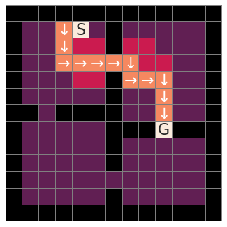
(a) AC trajectory

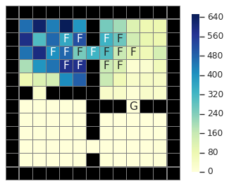
(b) AC variance

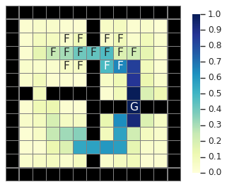
(c) AC frequency

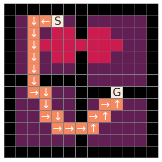
(d) VPAC trajectory

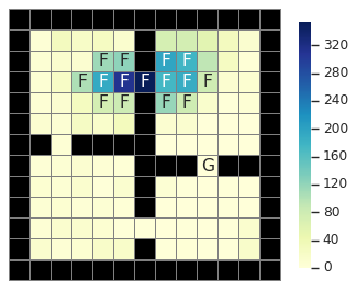
(e) VPAC variance

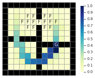
(f) VPAC frequency

Figure 1: Visualizations in four rooms: Qualitative analysis of converged policy’s behavior in AC and VPAC algorithms. AC algorithm: (a),(b),(c) Sampled trajectory, variance in return for initial state distribution, state visitation frequency over $10000$ trajectories respectively. Similarly, (d),(e),(f) depicts outcome on VPAC algorithm. $F$/ red region depicts the frozen states, $S$ the start state and $G$ the goal state. VPAC produces a lower variance in the return than AC by taking lower hallway to avoid the variable $F$ region.

Experiments

We present an empirical analysis in both discrete and continuous environments for the proposed on-policy and off-policy VPAC algorithms. We compare our algorithms with two baselines: AC and VAAC, an existing variance penalized actor-critic algorithm using an indirect variance estimator (Tamar and Mannor 2013) (refer Related Work section for further details). Given the penalty term is added to the objective function, we hypothesize that our approach should achieve a reduction in variance, but on-par average returns compared to the baselines. Implementation details along with the hyperparameters used for all the experiments are provided in Appendix E.

On-Policy Variance Penalized Actor-Critic (VPAC)

Tabular environment

We modify the classic four rooms (FR) environment (Sutton, Precup, and Singh 1999) to include a patch of frozen states (see Fig. 1) with stochastic reward. In the normal (non-frozen) states, the agent gets a reward of $0$, whereas in the frozen states, the reward is sampled from a normal distribution $\mathcal{N}(\mu=0,\sigma=8)$. Upon reaching the goal, a reward of $50$ is observed. Note that in expectation, the reward for the normal and the frozen states is the same. Hence, an agent that only optimizes expected return would have no reason to prefer some of these states over others. However, intuitively it would make sense to design agents that avoid the frozen states, which can be achieved by algorithms sensitive to the variance. We keep $\gamma=0.99$. We use Boltzmann exploration and do a grid search to find the best hyperparameters for all algorithms, where the least variance is used to break ties among policies with maximum mean performance. We show the impact of varying the hyperparameters on both the mean and the variance performance in Appendix E. We also show the table of best hyperparameters (found using grid search) used for all algorithms in Appendix E.

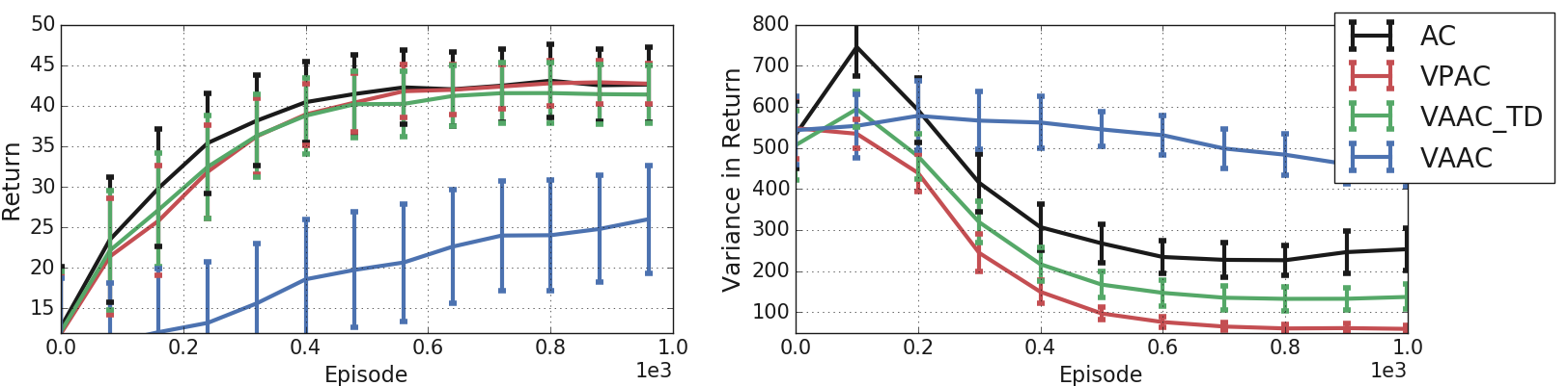
Figure 2: Performance in four rooms: Mean and variance performance comparison of our VPAC and baselines ( AC, VAAC, VAAC_TD) algorithms where standard deviation error-bars from $100$ runs are shown. VPAC achieves significantly lower variance in the return (right plot) while maintaining similar average return as the baselines (left plot).

In Fig. 2, we compare the mean and the variance in the return of the proposed Algorithm 1 VPAC and two other indirect variance penalized algorithms: Algorithm 2 VAAC (Tamar and Mannor 2013) (a Monte-Carlo critic update), and Algorithm 3 VAAC_TD (we modified VAAC to do a TD critic update for a fair comparison) and risk-neutral AC. Algorithms 2 and 3 are presented in Appendix E. The figure shows that VPAC has comparable mean performance to AC and less variance in return (red line). For all algorithms, we rolled out $800$ trajectories for each policy along the learning curve to calculate the variance in return. Note, here variance penalization does not highly impact the mean performance even though number of steps to reach the goal increases, because $\gamma=0.99$. In Fig. 3 we show the effect of varying the mean-variance tradeoff $\psi$ on both the mean and the variance performance of VPAC algorithm. This shows with very high values of $\psi$, the exploration is curbed causing a decay in the performance. In Appendix E, we show the sensitivity of VPAC and VAAC_TD with the step size ratios of policy, variance and value function. We empirically observe that keeping the step sizes of value and variance function closer to each other and the step size of policy very small in comparison to the other two, results in a better performance (both higher mean and lower variance).

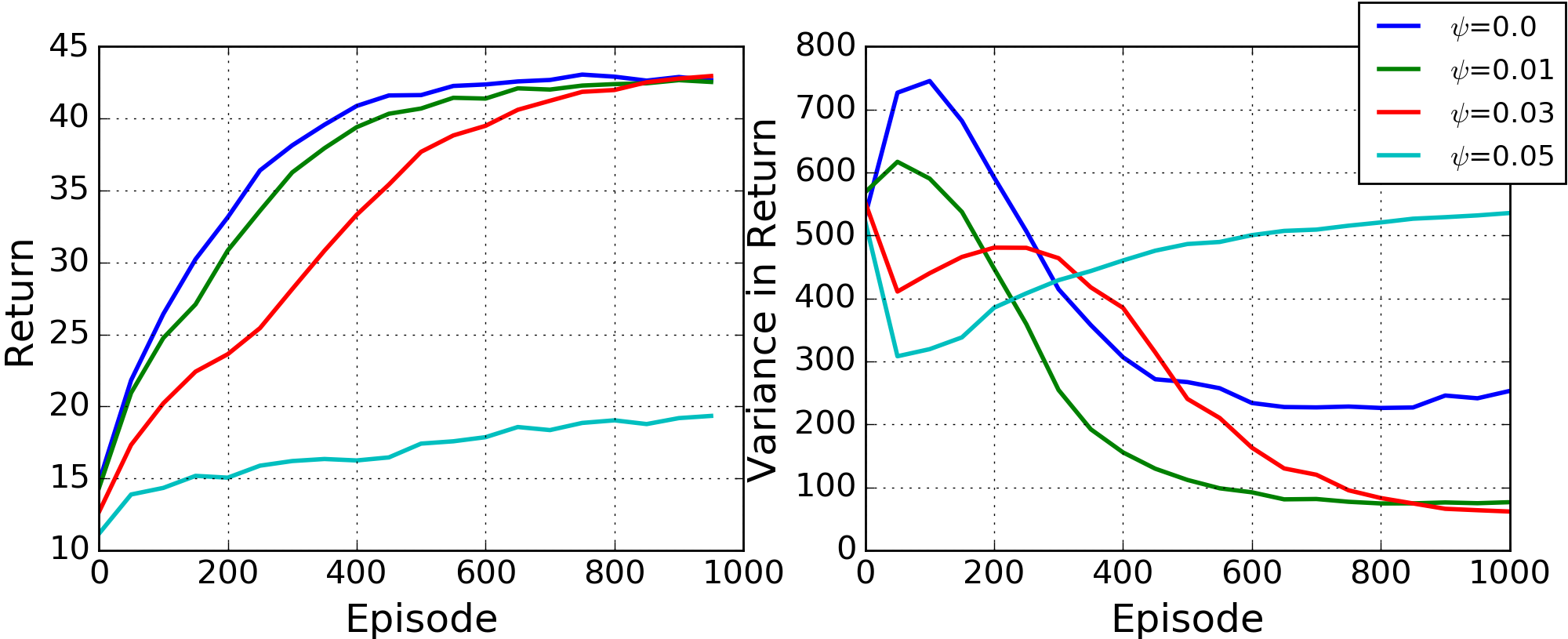
Figure 3: Mean-variance tradeoff ($\psi$) vs performance in four rooms: Plot shows VPAC’s learning curves for different values of $\psi$ in terms of the mean and the variance performance. The performance is averaged over $100$ runs.

Qualitative analysis: We compare AC and VPAC to analyse the learned policy’s behaviour. Fig. 1, (a) & (d), shows the sampled trajectory where VPAC clearly learns to avoid the variance-inducing frozen region. The variance in the return is depicted in Fig. 1, (b) & (e), where each cell color represents variance intensity in trajectories initialized from that cell. VPAC shows smaller variance compared to AC, and its trajectories avoid the $F$ region. This is further strengthened by Fig. 1, (c) & (f), showing the state visitation frequency, where VPAC has higher visitation frequency for the lower hallway. Fig. 4 shows the comparison between VPAC and VAAC_TD algorithm’s observed variance in return for a converged policy (obtained after $1000$ episodes) being initialized from each different states in the FR environment. Policy learnt using VPAC algorithm displays lower variance, highlighting better capability in learning and avoiding states that cause variability in the performance.

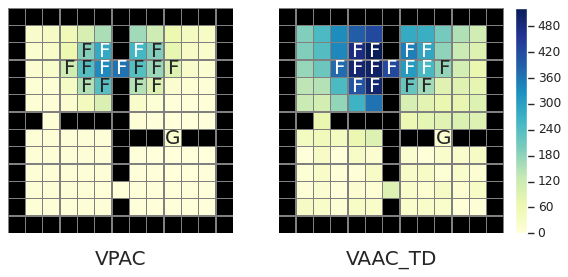
Figure 4: Comparison of variance in return for four rooms: Compares the converged policy’s variance in return for initial state distribution of VPAC and baseline VAAC_TD algorithm. The variance in performance over $5000$ trajectories is averaged over 50 runs. VPAC’s converged policy achieves significantly lower variance in return demonstrating the effectiveness in avoiding the variable $F$ region.

Continuous state-action environments

We now turn to continuous state-action tasks in the MuJoCo OpenAI Gym (Brockman et al. 2016). Note, here our aim is not to beat the mean performance with state-of-the-art PG methods, but to show the effect of introducing variance-penalization in a PG method. We can use the proposed objective with various existing PG methods, here, we limit our comparison with the proximal policy optimization (PPO) algorithm (Schulman et al. 2017).

A separate network for variance estimation is added in PPO to implement the variance-penalized objective function. Further details are provided in Appendix E. We compare the performance of our method VPAC with standard PPO and self-implemented VAAC in the PPO framework. Fig. 5 shows the box plot of the variance in the return for converged policies across multiple runs in Hopper, Walker2D, and HalfCheetah environments. As seen in the figure, a lowered concentration mass for the variance distribution is observed for VPAC in comparison to the baselines, supporting a reduction in the variance induced by the algorithm (see red median line and inter-quartile range). Table 1 shows the mean and the variance in return from $100$ rolled out trajectories of the converged policies of different algorithms. We averaged the above performance measure over multiple runs. Our method VPAC observes a reduction in the variance, but also suffers slightly in terms of mean performance. Note, Table 1 and Fig. 5 shows different metrics, mean and median of variance in performance respectively over multiple runs. The learning curve mean performance for different algorithms is shown in Appendix E.

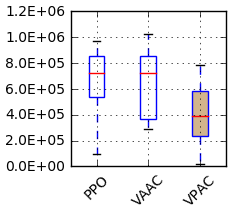
(a) Hopper

(b) Walker2D

(c) HalfCheetah

Figure 5: Variance analysis in Mujoco: The box plots show the distribution of variance in the return of converged policy across multiple runs for VPAC and baselines PPO and VAAC. Overall, in comparison to the baselines, VPAC exhibits a lowered, tighter distribution along with a reduction in the median of variance.

Table 1: Performance in Mujoco: Compares the averaged performance of PPO,VAAC,VPAC algorithms over multiple runs in terms of the mean and the variance in the score over $100$ trajectories. Bold highlights the least variance in the score. Numbers in braces show the percentage reduction of variance in comparison to PPO. VPAC achieves a lower variance in the score compared to the baselines, but also suffers slightly in terms of mean performance.

	PPO		VAAC		VPAC (ours)
Environment	Mean	Var (1e5)	Mean	Var (1e5)	Mean	Var (1e5)
HalfCheetah	1557	1.6	1525	0.8 (50%)	1373	0.1 (93%)
Hopper	1944	6.6	1991	6.5 (1.5%)	1624	4.0 (39.4%)
Walker2d	3058	12.1	3102	12.5 (-3.3%)	2625	9.2 (23.9%)

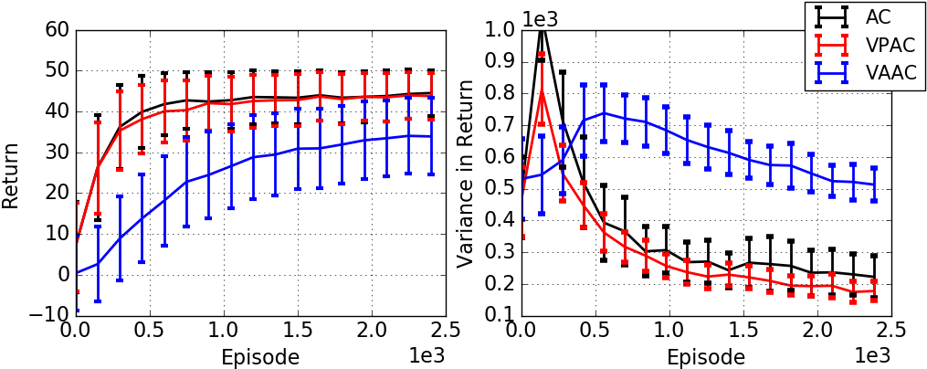
(a) Discrete puddle-world

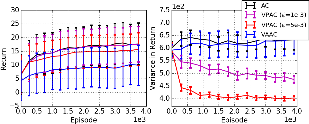
(b) Continuous puddle-world

Figure 6: Off-policy learning curves: Off-policy performance comparison over baselines AC, VAAC and VPAC averaged over $100$ trials a) discrete, and $50$ trials for b) continuous setting in puddle-world environment. The graph shows both the mean and the variance in return for the learnt target policy. $\psi$ is mean-variance tradeoff.

Off-Policy Variance-Penalized Actor-Critic (VPAC)

We compare off-policy VPAC with both VAAC (Tamar and Mannor 2013) and AC algorithms. Since VAAC is a on-policy AC algorithm, we modify it to its off-policy counterpart by appropriately incorporating an importance sampling correction factor. Note that, VAAC uses Monte-Carlo critic, whereas, AC and VPAC use TD critic. We left the comparison with off-policy version of VAAC_TD, since its derivation in AC was not straightforward.

Tabular environment

We investigate a modified puddle-world environment with a variable reward puddle region in the centre. The goal state $G$ is placed in the top right corner of the grid. The reward from normal and puddle region is same on expectation. Samples are generated from a uniform behavior policy. The target policy is a Boltzmann distribution over policy parameters. We use Retrace (Munos et al. 2016) for off-policy correction. Fig. 6(a) compares the mean and the variance in return of target policy for off-policy baselines AC,VAAC with VPAC. VPAC observes the least variance in the return, without sacrificing the mean performance. Fig. 7 (a),(b) compares a sampled trajectory for AC and VPAC. The baseline takes the shortest path to the goal, whereas, VPAC avoids the variable reward puddle region. The state visitation frequency plots are provided in Appendix E.

(a) Discrete AC

(b) Discrete VPAC

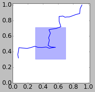
(c) Continuous AC

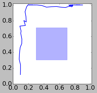
(d) Continuous VPAC

Figure 7: Off-policy puddle-world trajectories: Compares sampled trajectories for both off-policy AC and VPAC in {(a),(b)} discrete, and {(c),(d)} continuous puddle-world environment. VPAC avoids variable reward puddle region (shown in red/blue).

Continuous state environment

Next, we examine the performance of off-policy VPAC in continuous 2-D puddle-world environment similar to the discrete case, but with linear function approximation. We use tile coding (Sutton, Barto et al. 1998) for discretization of the state-space. Further experimental details are presented in Appendix E. Fig. 6(b), compares the mean and the variance performance of VPAC with the baselines. We observe a significant reduction in the variance for VPAC as compared to other baselines. In Fig. 6(b), as mean-variance tradeoff $\psi$ increases (compare pink and red lines), we observe not only substantially lower variance (right plot) for VPAC, but, also a slight reduction in the mean performance (left plot). This observation highlights that role of $\psi$ in the mean-variance tradeoff. Fig. 7 (c), (d) displays the sampled trajectories for AC and VPAC converged policies, highlighting VPAC avoids the variance inducing regions.

Related Work

There has been significant effort to reduce the variability in the performance of AI agents, by minimizing the risk in the form of exponential utility function (Howard and Matheson 1972; Borkar 2001; Basu, Bhattacharyya, and Borkar 2008; Nass, Belousov, and Peters 2019), Sharpe ratio (Sharpe 1994), worst-case outcome (Heger 1994; Mihatsch and Neuneier 2002), value-at-risk (VaR) (Duffie and Pan 1997), conditional-value-at-risk (CVaR) (Rockafellar, Uryasev et al. 2000; Chow and Ghavamzadeh 2014; Tamar, Glassner, and Mannor 2015), or variance (Markowitz 1959; Filar, Kallenberg, and Lee 1989; Sobel 1982; White 1994). Garcıa and Fernández (2015) provide a detailed analysis of different approaches to limit the variability. Although, many risk-sensitive RL methods have been introduced, variance based risk methods have an explicit advantage in being more interpretable (Markowitz and Todd 2000).

Our work involves mean-variance optimization, and therefore, we limit our discussion to variance-related risk measures. Sobel (1982) introduced an indirect approach to estimate the variance using the first and the second moments of return. Later, White and White (2016) extended the traditional indirect variance estimator to $\lambda$-returns. Indirect approaches to estimate the variance have been studied  (Tamar, Di Castro, and Mannor 2012; Tamar and Mannor 2013; Tamar, Di Castro, and Mannor 2013; Prashanth and Ghavamzadeh 2013, 2016) in many mean-variance optimization problems. Guo, Ye, and Yin (2012) studied mean-variance optimization, with the aim to minimize the variance, assuming access to already optimal expected reward, dealing with a much simpler problem than ours. In the episodic AC setting, Tamar and Mannor (2013) studied a variance-penalized method with an indirect approach to estimate the variance (using the second moment of return). Prashanth and Ghavamzadeh (2013; 2016) extended the indirect variance estimator to AC algorithm using simultaneous perturbation methods. Another risk-averse policy gradient method proposed by Bisi et al. (2019) measures risk using a different metric called reward volatility which captures the variance of the reward at each time step (as opposed to variance in return which measures variance in the accumulated rewards among trajectories). Reward constrained policy optimization (RCPO) (Tessler, Mankowitz, and Mannor 2019) approach uses a fixed constraint signal as a penalty in the reward function. In our work, we use varying variance in return as a constraint which depends on both the policy and $Q$ function, thus, making combined Bellman update for critic (value and variance) impossible unlike RCPO.

Thomas, Theocharous, and Ghavamzadeh (2015) estimated safety in the off-policy setting by bounding the probability of performance for a given confidence. White and White (2016), Sherstan et al. (2018) measured the variance for a target policy using off-policy samples in the policy evaluation setting. It is to be noted that an alternative approach to estimate the variance in return is by using the distribution over return (Morimura et al. 2010; Bellemare, Dabney, and Munos 2017).

Our work is closely related to Tamar and Mannor (2013), Prashanth and Ghavamzadeh (2013) and Sherstan et al. (2018). The former (Tamar and Mannor 2013; Prashanth and Ghavamzadeh 2013) developed an AC method for mean-variance optimization using the return’s first and second moments for variance estimation (an indirect variance computation approach described in Introduction). On the other hand, direct variance estimator proposed by Sherstan et al. for policy evaluation provides an alternative over indirect estimators. Our work is an extension to both of these methods, wherein, we propose a new AC algorithm which uses the TD style direct variance estimator (Sherstan et al. 2018) to compute a variance-penalized objective function in a control setting.

Conclusion & Future Work

We proposed an on- and off-policy actor-critic algorithm for variance penalized objective which leverages multi-timescale stochastic approximations, where both value and variance critics are estimated in TD style. We use the direct variance estimator for our proposed objective function. The empirical evidence in our work (see section Experiments) demonstrates that both our algorithms result in trajectories with much lower variance as compared to the risk-neutral and existing indirect variance-penalized counterparts.

Furthermore, we provided convergence guarantees for the proposed algorithm in the tabular case. Extending theoretical analysis to the linear function-approximation is a promising direction for future work. Another potential direction is to study the effects of a scheduler on the mean-variance tradeoff $\psi$, which can provide a balance between exploration at beginning and variance reduction towards the later stage.

References

- Altman (1999) Altman, E. 1999. Constrained Markov decision processes, volume 7. CRC Press.
- Basu, Bhattacharyya, and Borkar (2008) Basu, A.; Bhattacharyya, T.; and Borkar, V. S. 2008. A learning algorithm for risk-sensitive cost. Mathematics of operations research 33(4): 880–898.
- Bellemare, Dabney, and Munos (2017) Bellemare, M. G.; Dabney, W.; and Munos, R. 2017. A distributional perspective on reinforcement learning. In Proceedings of the 34th International Conference on Machine Learning-Volume 70, 449–458. JMLR. org.
- Bisi et al. (2019) Bisi, L.; Sabbioni, L.; Vittori, E.; Papini, M.; and Restelli, M. 2019. Risk-Averse Trust Region Optimization for Reward-Volatility Reduction. arXiv preprint arXiv:1912.03193 .
- Borkar (2001) Borkar, V. S. 2001. A sensitivity formula for risk-sensitive cost and the actor–critic algorithm. Systems & Control Letters 44(5): 339–346.
- Borkar (2002) Borkar, V. S. 2002. Q-learning for risk-sensitive control. Mathematics of operations research 27(2): 294–311.
- Borkar (2009) Borkar, V. S. 2009. Stochastic approximation: a dynamical systems viewpoint, volume 48. Springer.
- Brockman et al. (2016) Brockman, G.; Cheung, V.; Pettersson, L.; Schneider, J.; Schulman, J.; Tang, J.; and Zaremba, W. 2016. OpenAI gym. arXiv preprint arXiv:1606.01540 .
- Chow and Ghavamzadeh (2014) Chow, Y.; and Ghavamzadeh, M. 2014. Algorithms for CVaR optimization in MDPs. In Advances in Neural Information Processing Systems, 3509–3517.
- Duffie and Pan (1997) Duffie, D.; and Pan, J. 1997. An overview of Value at Risk. Journal of derivatives 4(3): 7–49.
- Filar, Kallenberg, and Lee (1989) Filar, J. A.; Kallenberg, L. C.; and Lee, H.-M. 1989. Variance-penalized Markov decision processes. Mathematics of Operations Research 14(1): 147–161.
- Garcıa and Fernández (2015) Garcıa, J.; and Fernández, F. 2015. A comprehensive survey on safe reinforcement learning. Journal of Machine Learning Research 16(1): 1437–1480.
- Guo, Ye, and Yin (2012) Guo, X.; Ye, L.; and Yin, G. 2012. A mean–variance optimization problem for discounted Markov decision processes. European Journal of Operational Research 220(2): 423–429.
- Heger (1994) Heger, M. 1994. Consideration of risk in reinforcement learning. In Machine Learning Proceedings 1994, 105–111. Elsevier.
- Howard and Matheson (1972) Howard, R. A.; and Matheson, J. E. 1972. Risk-sensitive Markov decision processes. Management science 18(7): 356–369.
- Iyengar (2005) Iyengar, G. N. 2005. Robust dynamic programming. Mathematics of Operations Research 30(2): 257–280.
- Konda and Tsitsiklis (2000) Konda, V. R.; and Tsitsiklis, J. N. 2000. Actor-critic algorithms. In Advances in Neural Information Processing Systems, 1008–1014.
- Markowitz (1959) Markowitz, H. 1959. Portfolio selection: Efficient diversification of investments, volume 16. John Wiley New York.
- Markowitz and Todd (2000) Markowitz, H. M.; and Todd, G. P. 2000. Mean-variance analysis in portfolio choice and capital markets, volume 66. John Wiley & Sons.
- Mihatsch and Neuneier (2002) Mihatsch, O.; and Neuneier, R. 2002. Risk-sensitive reinforcement learning. Machine learning 49(2-3): 267–290.
- Morimura et al. (2010) Morimura, T.; Sugiyama, M.; Kashima, H.; Hachiya, H.; and Tanaka, T. 2010. Parametric Return Density Estimation for Reinforcement Learning. In Proceedings of the Twenty-Sixth Conference on Uncertainty in Artificial Intelligence, UAI’10, 368–375.
- Munos et al. (2016) Munos, R.; Stepleton, T.; Harutyunyan, A.; and Bellemare, M. 2016. Safe and efficient off-policy reinforcement learning. In Advances in Neural Information Processing Systems, 1054–1062.
- Nass, Belousov, and Peters (2019) Nass, D.; Belousov, B.; and Peters, J. 2019. Entropic Risk Measure in Policy Search. In 2019 IEEE/RSJ International Conference on Intelligent Robots and Systems.
- Nilim and El Ghaoui (2005) Nilim, A.; and El Ghaoui, L. 2005. Robust control of Markov decision processes with uncertain transition matrices. Operations Research 53(5): 780–798.
- Prashanth and Ghavamzadeh (2013) Prashanth, L.; and Ghavamzadeh, M. 2013. Actor-critic algorithms for risk-sensitive MDPs. In Advances in Neural Information Processing Systems, 252–260.
- Prashanth and Ghavamzadeh (2016) Prashanth, L.; and Ghavamzadeh, M. 2016. Variance-constrained actor-critic algorithms for discounted and average reward MDPs. Machine Learning 105(3): 367–417.
- Rockafellar, Uryasev et al. (2000) Rockafellar, R. T.; Uryasev, S.; et al. 2000. Optimization of Conditional Value-at-Risk. Journal of risk 2: 21–42.
- Schulman et al. (2017) Schulman, J.; Wolski, F.; Dhariwal, P.; Radford, A.; and Klimov, O. 2017. Proximal policy optimization algorithms. arXiv preprint arXiv:1707.06347 .
- Sharpe (1994) Sharpe, W. F. 1994. The sharpe ratio. Journal of portfolio management 21(1): 49–58.
- Sherstan et al. (2018) Sherstan, C.; Ashley, D. R.; Bennett, B.; Young, K.; White, A.; White, M.; and Sutton, R. S. 2018. Comparing Direct and Indirect Temporal-Difference Methods for Estimating the Variance of the Return. In Proceedings of Uncertainty in Artificial Intelligence, 63–72.
- Sobel (1982) Sobel, M. J. 1982. The variance of discounted Markov decision processes. Journal of Applied Probability 19(4): 794–802.
- Sutton and Barto (2018) Sutton, R. S.; and Barto, A. G. 2018. Reinforcement learning: An introduction.
- Sutton, Barto et al. (1998) Sutton, R. S.; Barto, A. G.; et al. 1998. Reinforcement learning: An introduction. MIT press.
- Sutton et al. (2000) Sutton, R. S.; McAllester, D. A.; Singh, S. P.; and Mansour, Y. 2000. Policy gradient methods for reinforcement learning with function approximation. In Advances in Neural Information Processing Systems, 1057–1063.
- Sutton, Precup, and Singh (1999) Sutton, R. S.; Precup, D.; and Singh, S. 1999. Between MDPs and semi-MDPs: A framework for temporal abstraction in reinforcement learning. Artificial Intelligence 112(1-2): 181–211.
- Tamar, Di Castro, and Mannor (2012) Tamar, A.; Di Castro, D.; and Mannor, S. 2012. Policy gradients with variance related risk criteria. In Proceedings of the twenty-ninth International Conference on Machine Learning, 387–396.
- Tamar, Di Castro, and Mannor (2013) Tamar, A.; Di Castro, D.; and Mannor, S. 2013. Temporal difference methods for the variance of the reward to go. In International Conference on Machine Learning, 495–503.
- Tamar, Glassner, and Mannor (2015) Tamar, A.; Glassner, Y.; and Mannor, S. 2015. Optimizing the CVaR via sampling. In In Proceedings of the AAAI Conference on Artificial Intelligence (AAAI. Citeseer.
- Tamar and Mannor (2013) Tamar, A.; and Mannor, S. 2013. Variance adjusted actor critic algorithms. arXiv preprint arXiv:1310.3697 .
- Tessler, Mankowitz, and Mannor (2019) Tessler, C.; Mankowitz, D. J.; and Mannor, S. 2019. Reward Constrained Policy Optimization. In International Conference on Learning Representations.