Decoding of Quantum Data-Syndrome Codes via Belief Propagation

Abstract

Quantum error correction is necessary to protect logical quantum states and operations. However, no meaningful data protection can be made when the syndrome extraction is erroneous due to faulty measurement gates. Quantum data-syndrome (DS) codes are designed to protect the data qubits and syndrome bits concurrently. In this paper, we propose an efficient decoding algorithm for quantum DS codes with sparse check matrices. Based on a refined belief propagation (BP) decoding for stabilizer codes, we propose a DS-BP algorithm to handle the quaternary quantum data errors and binary syndrome bit errors. Moreover, a sparse quantum code may inherently be able to handle minor syndrome errors so that fewer redundant syndrome measurements are necessary. We demonstrate this with simulations on a quantum hypergraph-product code.

I Introduction

Quantum error-correction codes are indispensable in fault-tolerant quantum computation (FTQC) and quantum communication [1, 2, 3, 4]. Quantum stabilizer codes are an important class of quantum codes [5, 6, 7] since they allow simple encoding and decoding processes similar to classical error-correcting codes. This decoding process is analogous to the classical syndrome-based decoding. However, quantum operations are inevitably faulty, making robust syndrome extraction difficult. Using imperfect syndrome measurements, the outcome will be inaccurate and it may also corrupt the data qubits. As a consequence, we will be led into using a wrong syndrome, which will in turn provide us with an incorrect decoding result for error recovery.

Conventionally, an error recovery operation is chosen by repeated syndrome measurements, followed by a certain decision strategy [1]. For topological codes, the minimum-weight perfect-matching decoder is able to locate a likely error with high complexity [8]. For the ease of analysis, a simple error model is considered, where each qubit independently suffers a Pauli error and each syndrome bit independently suffers a bit-flip error. It has been shown that quantum stabilizer codes could be capable of correcting data errors and syndrome errors simultaneously, known as quantum data-syndrome (DS) codes [9, 10, 11, 12]. Recently, there has been a proposal put forward to construct quantum convolutional DS codes with a generalized Viterbi decoding algorithm [13]. Following Bombin’s seminal work on the single-shot fault-tolerant quantum error-correction to handle measurement errors, other approaches have also been proposed for topological codes [14, 15, 16].

We would like to develop a decoding algorithm with low complexity for FTQC by first studying the simple error model. In this paper we study the decoding of sparse-graph quantum codes [17, 18, 19] with independent data and syndrome errors using belief propagation (BP). BP has been shown to be powerful and efficient for classical decoding [20, 21], artificial intelligence decision [22], and quantum decoding [18, 23, 24]. Since the Pauli errors $\{I,X,Y,Z\}$ are quaternary but a syndrome bit-flip error is binary, a hybrid quaternary-binary nature of the DS codes is created, which makes their decoding complicated. Previously BP for quantum codes (BP₄) has been refined to pass only scalar messages because of the fact that the error syndromes for a stabilizer code are binary [24]. Accordingly, we propose a decoding algorithm (called DS-BP₄) for quantum DS codes, showing that the quaternary data error information and binary syndrome bit-flip information can be handled by scalar message passing.

A quantum DS code has additional redundant stabilizers being measured and usually a two-stage sequential decoding process is applied [9, 13]. In reality, syndrome measurements take a longer time than simple logical operations. One would like to have redundant measurements as few as possible. We demonstrate that DS-BP₄ on a quantum hypergraph-product (HP) code without any redundant syndrome bits may have performance close to the case of perfect syndrome measurements (where the loss in block error rate is less than an order for the $[[129,28]]$ HP code). On the other hand, we assume that the error rate is higher if repeated syndrome measurements are conducted since this usually takes a longer time. Then DS-BP₄ on the HP code without any redundant syndrome bits performs better than the two-stage sequential decoding.

The paper is organized as follows. In Sec. II, we introduce the basics of stabilizer codes and quantum DS codes. In Sec. III, a DS-BP₄ decoding algorithm for quantum DS codes is proposed along with the simulation results. Then we conclude in Sec. IV.

II Quantum Data-Syndrome Codes

II-A Quantum Stabilizer Codes

We consider binary stabilizer codes [5, 7]. Suppose that ${\cal S}$ is a subgroup of the $N$-fold Pauli group ${\cal G}_{N}$ and generated by $N-K$ independent $N$-fold Pauli operators $S_{1},S_{2},\dots,S_{N-K}$ such that $S_{m}S_{m^{\prime}}=S_{m^{\prime}}S_{m}$ and $-I^{\otimes N}\notin{\cal S}$. An $[[N,K]]$ stabilizer code $C({\cal S})$ encodes $K$ logical qubits into $N$ physical qubits and its code space is the joint $(+1)$ eigenspace of the elements in ${\cal S}$. The elements in ${\cal S}$ are called stabilizers. If a Pauli error anticommutes with some stabilizers, it can be detected by measuring the eigenvalues of the stabilizers. Thus the measurement outcomes, called error syndrome, are used to determine a correction operation. Sometimes additional redundant stabilizers $\{S_{m}\}_{m=N-K+1}^{M}$ are measured for enhancing BP in decoding [25] or handling syndrome errors [11, 12].

Without loss of generality, $S_{m}$ is of the form $S_{m}=S_{m1}\otimes S_{m2}\otimes\dots\otimes S_{mN},$ where $S_{mn}\in\{I=[{1\atop 0}{0\atop 1}],X=[{0\atop 1}{1\atop 0}],Z=[{1\atop 0}{0\atop-1}],Y=iXZ\}$ for $n=1,2,\dots,N$. We will ignore the notation $\otimes$ without confusion. Then

$$S=[S_{mn}]\in\{I,X,Y,Z\}^{M\times N}$$

is called the check matrix of the stabilizer code. Two Pauli operators of the same dimension, $E$ and $F$, either commute or anticommute with each other. We define

$$\langle E,F\rangle_{{\cal G}}=\begin{cases}0,&\mbox{if $EF=FE$};\\ 1,&\mbox{otherwise}.\end{cases}$$ (1)

For an error $E=E_{1}E_{2}\cdots E_{N}\in{\cal G}_{N}$, its binary error syndrome is given by $z=(z_{1},z_{2},\dots,z_{M})\in\{0,1\}^{M}$, where

$$z_{m}=\langle E,S_{m}\rangle_{{\cal G}}=\sum_{n=1}^{N}\langle E_{n},S_{mn}\rangle_{{\cal G}}\mod 2.$$

Let $\operatorname{wt}_{\cal G}(E)$ denote the number of non-identity entries in $E\in{\cal G}_{N}$. The minimum distance of $C({\cal S})$ is defined as

$$d=\min\{\operatorname{wt}_{\cal G}(E)\mid E\in\{I,X,Y,Z\}^{N}\setminus{\cal S},\,\langle E,S_{m}\rangle=0~{}\forall~{}m\}.$$

A stabilizer code with minimum distance $d$ can correct any errors $E$ with $\operatorname{wt}_{\cal G}(E)\leq t$, where $t=\lfloor\frac{d-1}{2}\rfloor$.

II-B Quantum Data-Syndrome (DS) Codes

In addition to a Pauli error $E\in{\cal G}_{N}$ on the data qubits, each syndrome bit $z_{m}$ suffers an independent bit-flip error $e_{m}\in\{0,1\}$. Now the syndrome bit relation becomes

$$z_{m}=\langle E,S_{m}\rangle_{{\cal G}}+e_{m}\mod 2.$$ (2)

Consequently the check matrix for the DS code is defined by

$$\tilde{S}=[S~{}I_{M}],$$ (3)

where $I_{M}$ is an $M\times M$ binary identity matrix. The $m$-th row of $\tilde{S}$ is denoted by $\tilde{S}_{m}=(S_{m},(I_{M})_{m})~{}\in~{}\{I,X,Y,Z\}^{N}\times\{0,1\}^{M}$. Define the product of $e,f\in\{0,1\}^{M}$ by $\langle e,f\rangle_{b}=\sum_{j=1}^{M}e_{j}f_{j}\mod 2.$ Then the product of $(E,e),(F,f)\in{\cal G}_{N}\times\{0,1\}^{M}$ is defined by

$$\langle(E,e),(F,f)\rangle=\langle E,F\rangle_{{\cal G}}+\langle e,f\rangle_{b}\mod 2.$$ (4)

For $e\in\{0,1\}^{M}$, let $\operatorname{wt}_{b}(e)$ denote the number of its nonzero entries. Then the weight of $(E,e)$ is defined as

$$\operatorname{wt}(E,e)=\operatorname{wt}_{\cal G}(E)+\operatorname{wt}_{b}(e).$$

Definition 1.

Let $S\in\{I,X,Y,Z\}^{M\times N}$ be a check matrix of an $[[N,K]]$ stabilizer code, where $M\geq N-K$. We say that $S$ induces an $[[N,K\,|\,M]]$ quantum DS code $\tilde{{\cal C}}$ with a DS check matrix $\tilde{S}=[S~{}I_{M}]$, where

$$\tilde{{\cal C}}=\{(F,f)\in\{I,X,Y,Z\}^{N}\times\{0,1\}^{M}\mid\langle(F,f),\tilde{S}_{m}\rangle=0~{}\forall~{}m\}.$$

The (DS) minimum distance of $\tilde{{\cal C}}$ is defined as

$$\tilde{d}=\min\{\operatorname{wt}(F,f)\mid(F,f)\in\tilde{{\cal C}}\setminus\tilde{{\cal S}}\},$$

where $\tilde{{\cal S}}\triangleq\{(F,\boldsymbol{0})\mid F\in{\cal S}\}$.

Theorem 1.

[12] An $[[N,K\,|\,M]]$ quantum DS code with DS minimum distance $\tilde{d}$ can correct any error $(E,e)\in{\cal G}_{N}\times\{0,1\}^{M}$ with $\operatorname{wt}(E,e)\leq\tilde{t}$, where $\tilde{t}=\lfloor\frac{\tilde{d}-1}{2}\rfloor$.

III Belief Propagation for Quantum DS Codes

The minimum distance $d$ of a stabilizer code is an upper bound on its induced DS minimum distance $\tilde{d}$. The DS minimum distance usually achieves this upper bound by additional redundant measurements [11, 12, 13].

In some conditions, we can have the syndrome protected without redundant measurements [10] and this is a desired property especially when the syndrome measurements are expensive: the syndrome error rate could be higher than the data error rate since a syndrome measurement involves many two-qubit operations and single qubit measurements; also more syndrome measurements take more processing time, which in turn incurs a higher data error rate.

In the next section, we will simulate a case of CSS codes [26, 27] since they are commonly used in FTQC. The stabilizer group of a CSS code can be chosen to be products of only $X$ operators or only $Z$ operators. Thus we have a binary check matrix $\textstyle H=[{H_{X}\atop O}\mid{O\atop H_{Z}}],$ where $H_{X}\in\{0,1\}^{M_{1}\times N}$, $H_{Z}\in\{0,1\}^{M_{2}\times N}$, $M=M_{1}+M_{2}$, and $H_{X}H_{Z}^{T}=O$, where $O$ is the all-zero matrix whose dimension can be inferred from the context. The induced quantum DS code has a (binary) check matrix:

$$\tilde{H}=\textstyle[{H_{X}\atop O}{I_{M_{1}}\atop O}\mid{O\atop H_{Z}}{O\atop I_{M_{2}}}].$$ (5)

It is not hard to obtain the following theorem.

Theorem 2.

Let $\tilde{H}$ be defined as in (5), where $H_{X}$ and $H_{Z}$ are the parity-check matrices of two classical codes, respectively, each with minimum distance at least 3. If every column of $H_{X}$ and $H_{Z}$ is of weight at least 2, then the induced quantum DS code has minimum distance at least 3.

The conditions can be generalized for higher-weight errors but it is complicated. We remark that the minimum distance of a code provides only a reference for its error performance; we care more about the following practical decoding problem:

The quantum DS decoding problem: Given a DS check matrix $\tilde{S}=[S~{}I_{M}]$, where $S\in\{I,X,Y,Z\}^{M\times N}$, a binary syndrome $z\in\{0,1\}^{M}$ of $(E,e)\in{\cal G}_{N}\times\{0,1\}^{M}$, and certain characteristics of the error model, the decoder has to infer $(\hat{E},\hat{e})$, where $\hat{E}\in\{I,X,Y,Z\}^{N}$ and $\hat{e}\in\{0,1\}^{M}$ such that $\langle(\hat{E},\hat{e}),\tilde{S}_{m}\rangle=z_{m}$ for all $m=1,2,\dots,M$ and $\hat{E}\in E{\cal S}$.

III-A The DS-BP Algorithm

We would like to have a successful decoding with probability as high as possible (according to a specific error model). In general, achieving an optimum decoding is extremely difficult for conventional stabilizer codes [28, 29] and this is also the case for DS codes. However, if $S$ is a sparse matrix, then $\tilde{S}$ is also sparse. Using BP to decode DS codes is also efficient and possible to have good performance like stabilizer codes [18, 23, 24].

The DS check matrix $\tilde{S}=[S~{}I_{M}]$ corresponds to a Tanner graph consisting of $N$ data(-variable) nodes, $M$ syndrome(-variable) nodes, and $M$ check nodes. There is an edge connecting data node $n$ and check node $m$ if $S_{mn}\neq I$. There is always an edge connecting check node $m$ and syndrome node $m$. For example, if $S=[{X\atop Z}{Y\atop Z}{I\atop Y}]$, then $\tilde{S}=[S~{}I_{M}]=[{X\atop Z}{Y\atop Z}{I\atop Y}{1\atop 0}{0\atop 1}]$ and its corresponding Tanner graph is shown in Fig. 1.

Figure 1: The Tanner graph of $\tilde{S}=[{X\atop Z}{Y\atop Z}{I\atop Y}{1\atop 0}{0\atop 1}]$. There are three types of edges connecting a data node and a check node.

Suppose that the data nodes and syndrome nodes are numbered from $1$ to $N+M$. Let ${\cal M}(n)$ be the neighboring check nodes of a variable node $n$, and ${\cal N}(m)$ be the neighboring variable nodes of a check node $m$. Using a similar derivation in [24, Algorithm 3] (or more simply, in [30]), it is not so difficult to generalize the quaternary BP (BP₄) algorithm for stabilizer codes [24, Algorithm 3] to DS-BP₄ for quantum DS codes as in Algorithm 1 that handles only scalar messages.

The initial probabilities of data and syndrome errors can be assigned in DS-BP₄. Suppose that each qubit suffers a memoryless depolarizing channel of depolarizing rate $\epsilon_{D}$ and each syndrome bit suffers a memoryless binary symmetric channel (BSC) of crossover rate $\epsilon_{S}$. Then $(p_{n}^{I},p_{n}^{X},p_{n}^{Y},p_{n}^{Z})$ are initialized to $(1-\epsilon_{D},\frac{\epsilon_{D}}{3},\frac{\epsilon_{D}}{3},\frac{\epsilon_{D}}{3})$ for each data-variable node $n\in\{1,\dots,N\}$, and $(p_{n}^{(0)},p_{n}^{(1)})$ are initialized to $(1-\epsilon_{S},\epsilon_{S})$ for each syndrome-variable node $n\in\{N+1,\dots,N+M\}$.

Algorithm 1 : Quaternary DS-BP decoding for quantum DS codes with a parallel schedule (parallel DS-BP₄)

Input: $\tilde{S}=[S\ I_{M}]$, ${S}\in\{I,X,Y,Z\}^{M\times N}$,  $z\in\{0,1\}^{M}$, and initial $\{(p_{n}^{I},p_{n}^{X},p_{n}^{Y},p_{n}^{Z})\}_{n=1}^{N},\{(p_{n}^{(1)},p_{n}^{(0)})\}_{n=N+1}^{N+M}$.
Initialization. For all $n=1$ to $N+M$ and all $m\in{\cal M}(n)$:

• If $n\leq N$, let $q_{mn}^{W}=p_{n}^{W}$ for $W\in\{I,X,Y,Z\}$,
  and let $q_{mn}^{(0)}=q_{mn}^{I}+q_{mn}^{S_{mn}}$ and $q_{mn}^{(1)}=1-q_{mn}^{(0)}$.

• If $n>N$, let $q_{mn}^{(0)}=p_{n}^{(0)}$ and $q_{mn}^{(1)}=p_{n}^{(1)}$.

• Calculate

  $$d_{n\to m}=q_{mn}^{(0)}-q_{mn}^{(1)}.$$ (6)

Horizontal Step. For all $m=1$ to $M$ and all $n\in{\cal N}(m)$:

• Compute

  $$\delta_{m\to n}=(-1)^{z_{m}}\prod_{n^{\prime}\in{\cal N}(m)\setminus n}d_{mn^{\prime}}.$$ (7)

Vertical Step. For all $n=1$ to $N+M$ and all $m\in{\cal M}(n)$:

• Let $r_{mn}^{(0)}=(1+\delta_{mn})/2$ and $r_{mn}^{(1)}=(1-\delta_{mn})/2$.

• If $n\leq N$, compute

  $$q_{mn}^{W} =p_{n}^{W}\prod_{m^{\prime}\in{\cal M}(n)\setminus m}r_{m^{\prime}n}^{(\langle W,S_{m^{\prime}n}\rangle)},~{}~{}W\in\{I,X,Y,Z\},$$ (8)

  $$q_{mn}^{(0)} =a_{mn}(q_{mn}^{I}+q_{mn}^{S_{mn}}),$$

  $$q_{mn}^{(1)} =a_{mn}(\textstyle\sum_{W^{\prime}\in\{X,Y,Z\}\setminus S_{mn}}q_{mn}^{W^{\prime}}).$$

• If $n>N$, compute

  $$q_{mn}^{(b)} =a_{mn}\,p_{n}^{(b)}\prod_{m^{\prime}\in{\cal M}(n)\setminus m}r_{m^{\prime}n}^{(b)},~{}~{}b\in\{0,1\}.$$ (9)

• Each $a_{mn}$ is a chosen scalar such that $q_{mn}^{(0)}+q_{mn}^{(1)}=1$.

• Update: $d_{n\to m}=q_{mn}^{(0)}-q_{mn}^{(1)}$.

Hard Decision. For all $n=1$ to $N+M$:

• If $n\leq N$, compute

  $$q_{n}^{W} =p_{n}^{W}\prod_{m\in{\cal M}(n)}r_{mn}^{(\langle W,S_{mn}\rangle)},~{}~{}W\in\{I,X,Y,Z\},$$

  and let $\hat{E}_{n}=\operatorname*{arg\,max}_{W\in\{I,X,Y,Z\}}q_{n}^{W}.$

• If $n>N$, compute

  $$q_{n}^{(b)} =p_{n}^{(b)}\prod_{m\in{\cal M}(n)}r_{mn}^{(b)},~{}~{}b\in\{0,1\},$$

  and let $\hat{e}_{n}=0$, if $q_{n}^{(0)}>q_{n}^{(1)}$, and $\hat{e}_{n}=1$, otherwise.

• Let $\hat{E}=\hat{E}_{1}\hat{E}_{2}\cdots\hat{E}_{N}$ and $\hat{e}=(\hat{e}_{N+1},\hat{e}_{N+2},\dots,\hat{e}_{N+M})$.

  • If $\langle(\hat{E},\hat{e}),\tilde{S}_{m}\rangle=z_{m}$ for all $m=1$ to $M$, halt and return “CONVERGED”.

  • Otherwise, if a maximum number of iterations is reached, halt and return “FAIL”.

  • Otherwise, repeat from the horizontal step.

Algorithm 1 performs the update according to a parallel schedule [24] and is referred to as parallel DS-BP₄. We also consider an update order according to a serial schedule running along the check nodes as in Algorithm 2, which is referred to as serial DS-BP₄. Consider the example in Fig. 1 again. Its message update order using parallel DS-BP₄ (resp. serial DS-BP₄) is illustrated in Fig. 2 (resp. Fig. 3). The message update order plays an important role in BP, especially when the Tanner graph has numerous short cycles [24, 31].

Algorithm 2 : Quaternary DS-BP decoding with a serial schedule along the check nodes (serial DS-BP₄)

Input: The same as in Algorithm 1.
Initialization. For all $m=1$ to $M$ and all $n\in{\cal N}(m)$:

• Let $\delta_{m\to n}=0$.

Serial Update. For each check node $m=1$ to $M$:

• For every $n\in{\cal N}(m)$, do the same as in the five bullet points around (8) and (9), with the order specified here.

• For every $n\in{\cal N}(m)$, compute

  $$\delta_{m\to n}=(-1)^{z_{m}}\prod_{n^{\prime}\in{\cal N}(m)\setminus n}d_{mn^{\prime}}.$$ (10)

Hard Decision.

• Do as in Algorithm 1, except that “repeat from the horizontal step" must be replaced by “repeat from the serial update step".

((a))

((b))

Figure 2: The message update order of parallel DS-BP₄ for the example in Fig. 1. (a) The initialization step, as well as the vertical step. (b) The horizontal step. The message update order will be iterated between (a) and (b).

((a))

((b))

((c))

((d))

Figure 3: The message update order of serial DS-BP₄ (along check nodes) for the example in Fig. 1. (a) and (b): serial update for check node 1. (c) and (d): serial update for check node 2. The message update order will be iterated from (a) to (d).

III-B Simulation Results

We construct a $[[129,28]]$ CSS-type HP code [19] based on the $[7,4,3]$ and $[15,7,5]$ BCH codes as in [32, 24]. This code has minimum distance $d=3$ and can be a candidate for Theorem 2. Its raw check matrix has some columns of weight one. After row multiplications by adjacent rows, we can obtain a check matrix, each column of which is of weight at least 2. Then by Theorem 2, we have a $[[129,28\,|\,101]]$ quantum HP DS code with minimum distance $\tilde{d}=3$.

We first explain the serial schedule that will be conducted in the following simulations. In [24], it is demonstrated that based on the raw check matrix of the $[[129,28]]$ HP code, the parallel BP₄ decoding does not perform well due to decoding oscillation (which is caused by the numerous short cycles and symmetric sub-graphs in the Tanner graph [24, 31]); on the other hand, the serial BP₄ along variable nodes performs quite well by using the raw matrix [24]. We have created a check matrix so that each of its column has weight $\geq 2$ for Theorem 2; however, the serial update along variable nodes is too aggressive at certain variable node for the new check matrix (when computing the hard-decision and outgoing messages). This causes for some weight-one errors to be decoded as weight-three errors, and the syndrome is falsely matched. Fortunately, this can be improved by using a serial update along the check nodes (which also breaks the symmetry in the short cycles and sub-graphs; however, it provides a more gradual update for each coordinate $n$ at each iteration).

In this subsection, the simulation of BP allows a maximum number of 12 iterations, and each data point is based on collecting at least 100 blocks of logical errors.

We begin with the simulation without syndrome errors ($\epsilon_{S}=0$) and compare the decoding results of parallel DS-BP₄ (Algorithm 1) and serial DS-BP₄ (Algorithm 2). In this case, DS-BP₄ is equivalent to the usual BP₄ in [24].

We use bounded-distance decoding (BDD) as a benchmark for error performance. In general, BDD with radius $t$ can correct any error of weight no larger than $t$. We consider a more general BDD as follows. Let $t\geq 0$ and $\gamma=(\gamma_{0},\gamma_{1},\dots,\gamma_{t})$, where $\gamma_{j}$ denotes the percentage of weight-$j$ errors assumed to be corrected. Then the generalized BDD with respect to $t$ and $\gamma$ has a logical error rate at $\epsilon$ ($=\epsilon_{D}$ here) as follows

$$P_{\text{e,BDD}}(N,t,\gamma)=1-\textstyle\left(\sum_{j=0}^{t}\gamma_{j}\binom{N}{j}\epsilon^{j}(1-\epsilon)^{(N-j)}\right).$$ (11)

The $[[129,28]]$ code can correct any error of weight one. If we make a lookup table for decoding by assigning each syndrome to low-weight errors, then this code can correct about $98.73\%$ of the weight-2 errors. Thus, with $t=2$, this lookup-table decoding provides a generalized BDD to have $\gamma_{0}=1,~{}\gamma_{1}=1,\text{ and }\gamma_{2}\approx 98.73\%.$ This code is not degenerate; its stabilizers have weight larger than 3. Consequently these three $\gamma_{j}$ values are fixed whether the degeneracy is considered or not, and they dominate the error performance.

Figure 4 shows the simulations of Algorithm 1 and Algorithm 2 at $\epsilon_{S}=0$, together with several BDD reference curves. Note that $\gamma_{j}=1$ for $j\leq t$ if not specified. Serial DS-BP₄ achieves a performance quite close to the lookup-table decoder $P_{\text{e,BDD}}(N,2,\gamma_{2}=98.73\%)$. This matches Gallager’s expectation that the performance of BP can be as close as to two times of the BDD performance with radius $t=\frac{d-1}{2}$ [20].

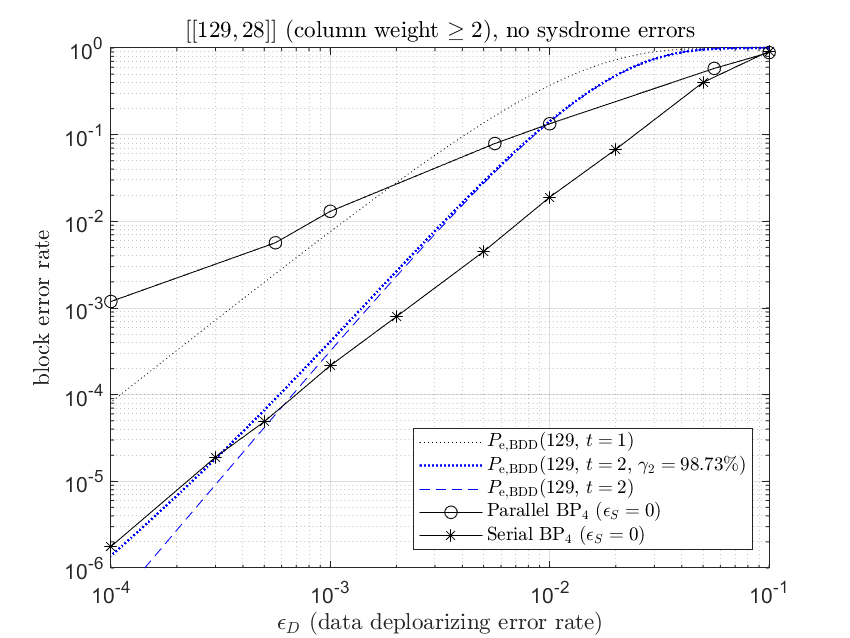
Figure 4: Decoding performance of the $[[129,28]]$ HP code (with syndrome error rate $\epsilon_{S}=0$). The serial schedule is along the check nodes. Specific BDD reference performance curves, per (11), are plotted.

Next, we assume that each syndrome bit is flipped with rate $\epsilon_{S}\neq 0$. For simplicity, assume $\epsilon_{S}=\epsilon_{D}$, which allows us to use (11) as a benchmark. We focus on the serial schedule since it provides a better performance. The serial DS-BP₄ performance is plotted in Fig. 5, which has a performance loss of less than an order compared to the case of no syndrome error $\epsilon_{S}=0$. It can be seen that serial DS-BP₄ improves serial BP₄ ($\epsilon_{S}=\epsilon_{D}$) if no repeated measurements are conducted as expected. We also provide a curve for serial BP₄ ($\epsilon_{S}=\epsilon_{D}$) with $r=3$ repeated measurements, and it performs quite well as seen in Fig. 5; however, this only reveals the importance of eliminating the effect caused by noisy measurements.

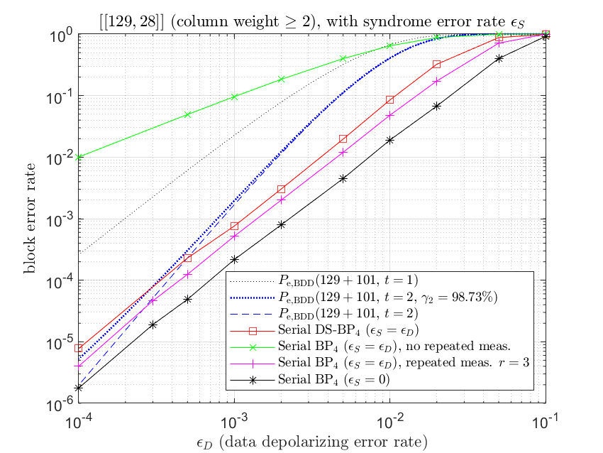
Figure 5: Decoding performance of the $[[129,28\,|\,101]]$ HP DS code. All the serial-schedule results are based on Algorithm 2. When it is labeled with “Serial BP₄”, it means that Algorithm 2 is run with $\epsilon_{S}=0$ regardless of the actual $\epsilon_{S}$ value. If there are $r$ repeated measurements (meas.), a majority vote will be run to decide the syndrome before running the decoding algorithm.

Performing repeated measurements would require additional time (and gates), so these practical issues should be considered in comparison. As described in [33, 34], the fidelity of a physical qubit decays exponentially over the operational time $\tau$. Assume that the fidelity is

$$1-\epsilon=e^{-\lambda\tau}$$ (12)

for some decay factor $\lambda$. Suppose that a round of syndrome measurement takes 740 ns [35]. We further assume that the measurement time dominates the overall error-correction time, since the decoder should run much faster in a classical hardware [36]. So now one round of measurements with one round of serial DS-BP₄ takes about $740$ ns, and $r=3$ rounds of measurements with one round of serial BP₄ takes about $3\times 740$ ns. Given $\epsilon$ ($=\epsilon_{D}$ in Fig. 5) and $\tau$ ($=740$ or $3\times 740$ ns), a corresponding $\lambda$ in (12) can be derived. Figure 6 provides the rescaled curves of Fig. 5. The results show that using the DS-BP approach can take the advantage of less measurement time to outperform a decoding strategy with repeated measurements.

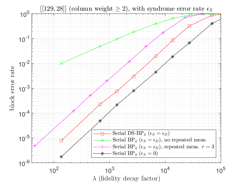
Figure 6: Comparing the different decoding strategies in Fig. 5, at a certain fidelity decay factor $\lambda$ as in (12), in which we assume that $\epsilon=\epsilon_{D}$ and $\tau=r\times 740$ ns (where there is only one case with $r=3$, as labeled, and the other cases have $r=1$).

IV Conclusion & Future Works

Faulty syndrome measurement is an issue that cannot be neglected in fault-tolerant quantum error-correction. A potential solution is to apply quantum DS codes. By generalizing the refined BP₄ [24], we proposed a DS-BP₄ decoding algorithm and have demonstrated that it can efficiently achieve satisfactory results. The DS-BP approach has proved to be suitable for low-weight stabilizers and can be used with less (or even without) redundant measurements. This decreases the measurement time and increases the probability of a successful decoding.

We simulated the $[[129,28\,|\,101]]$ HP DS code with minimum distance 3. For codes with higher minimum distance, we may use additional syndrome measurements to compensate the effects of syndrome errors. For example, the surface codes are the current state-of-the-art candidate for FTQC. It is still unknown whether BP works for codes with strong degeneracy that their stabilizers may have weight much lower than the minimum distance. Also, the error model considered in this paper is too ideal. To apply the DS-BP approach in a more practical model, like the faulty circuit model [8, 13], is our ongoing research.

References

- [1] P. W. Shor, “Fault-tolerant quantum computation,” in Proc. 37th Annu. Conf. Found. Comput. Sci. (FOCS), pp. 56–65, IEEE, 1996.
- [2] E. Knill and R. Laflamme, “Theory of quantum error-correcting codes,” Phys. Rev. A, vol. 55, p. 900, 1997.
- [3] A. M. Steane, “A tutorial on quantum error correction,” in Proc. Int. School Phys. Enrico Fermi, vol. 162, p. 1, IOS Press; Ohmsha; 1999, 2007.
- [4] D. A. Lidar and T. A. Brun, Quantum error correction. Cambridge University press, 2013.
- [5] D. Gottesman, Stabilizer codes and quantum error correction. PhD thesis, California Institute of Technology, 1997.
- [6] A. R. Calderbank, E. M. Rains, P. W. Shor, and N. J. A. Sloane, “Quantum error correction via codes over GF(4),” IEEE Trans. Inf. Theory, vol. 44, pp. 1369–1387, 1998.
- [7] M. A. Nielsen and I. Chuang, “Quantum computation and quantum information,” 2000.
- [8] A. G. Fowler, M. Mariantoni, J. M. Martinis, and A. N. Cleland, “Surface codes: Towards practical large-scale quantum computation,” Phys. Rev. A, vol. 86, p. 032324, 2012.
- [9] A. Ashikhmin, C.-Y. Lai, and T. A. Brun, “Robust quantum error syndrome extraction by classical coding,” in Proc. IEEE Int. Symp. Inf. Theory (ISIT), pp. 546–550, IEEE, 2014.
- [10] Y. Fujiwara, “Ability of stabilizer quantum error correction to protect itself from its own imperfection,” vol. 90, p. 062304, Dec 2014.
- [11] A. Ashikhmin, C.-Y. Lai, and T. A. Brun, “Correction of data and syndrome errors by stabilizer codes,” in Proc. IEEE Int. Symp. Inf. Theory (ISIT), pp. 2274–2278, IEEE, 2016.
- [12] A. Ashikhmin, C.-Y. Lai, and T. A. Brun, “Quantum data-syndrome codes,” IEEE J. Sel. Areas Commun., vol. 38, pp. 449–462, 2020.
- [13] W. Zeng, A. Ashikhmin, M. Woolls, and L. P. Pryadko, “Quantum convolutional data-syndrome codes,” in Proc. IEEE Int. Workshop Signal Process. Adv Wireless Commun. (SPAWC), pp. 1–5, 2019.
- [14] H. Bombín, “Single-shot fault-tolerant quantum error correction,” Phys. Rev. X, vol. 5, p. 031043, 2015.
- [15] B. J. Brown, N. H. Nickerson, and D. E. Browne, “Fault-tolerant error correction with the gauge color code,” Nat. Commun., vol. 7, pp. 1–8, 2016.
- [16] N. P. Breuckmann, K. Duivenvoorden, D. Michels, and B. M. Terhal, “Local decoders for the 2D and 4D toric code,” Quantum Inf. Comput., vol. 17, p. 181–208, 2016.
- [17] A. Y. Kitaev, “Fault-tolerant quantum computation by anyons,” Ann. Phys., vol. 303, pp. 2–30, 2003.
- [18] D. J. C. MacKay, G. Mitchison, and P. L. McFadden, “Sparse-graph codes for quantum error correction,” IEEE Trans. Inf. Theory, vol. 50, pp. 2315–2330, 2004.
- [19] J.-P. Tillich and G. Zémor, “Quantum LDPC codes with positive rate and minimum distance proportional to the square root of the blocklength,” IEEE Trans. Inf. Theory, vol. 60, pp. 1193–1202, 2014.
- [20] R. G. Gallager, Low-Density Parity-Check Codes. no. 21 in Research Monograph Series, Cambridge, MA: MIT Press, 1963.
- [21] D. J. C. MacKay, “Good error-correcting codes based on very sparse matrices,” IEEE Trans. Inf. Theory, vol. 45, pp. 399–431, 1999.
- [22] J. Pearl, Probabilistic reasoning in intelligent systems: networks of plausible inference. Morgan Kaufmann, 1988.
- [23] D. Poulin and Y. Chung, “On the iterative decoding of sparse quantum codes,” Quant. Inf. Comput., vol. 8, pp. 987–1000, 2008.
- [24] K.-Y. Kuo and C.-Y. Lai, “Refined belief propagation decoding of sparse-graph quantum codes,” IEEE J. Sel. Areas Inf. Theory, vol. 1, pp. 487–498, 2020.
- [25] A. Rigby, J. C. Olivier, and P. Jarvis, “Modified belief propagation decoders for quantum low-density parity-check codes,” Phys. Rev. A, vol. 100, p. 012330, 2019.
- [26] A. R. Calderbank and P. W. Shor, “Good quantum error-correcting codes exist,” Phys. Rev. A, vol. 54, p. 1098, 1996.
- [27] A. M. Steane, “Error correcting codes in quantum theory,” Phys. Rev. Lett., vol. 77, p. 793, 1996.
- [28] K.-Y. Kuo and C.-C. Lu, “On the hardnesses of several quantum decoding problems,” Quant. Inf. Process., vol. 19, pp. 1–17, 2020.
- [29] P. Iyer and D. Poulin, “Hardness of decoding quantum stabilizer codes,” IEEE Trans. Inf. Theory, vol. 61, pp. 5209–5223, 2015.
- [30] K.-Y. Kuo and C.-Y. Lai, “Refined belief-propagation decoding of quantum codes with scalar messages,” in Proc. IEEE Global Commun. Conf. (GLOBECOM), to be appeared, 2020.
- [31] N. Raveendran and B. Vasić, “Trapping sets of quantum LDPC codes,” e-print arXiv:2012.15297, 2020.
- [32] Y.-H. Liu and D. Poulin, “Neural belief-propagation decoders for quantum error-correcting codes,” Phys. Rev. Lett., vol. 122, p. 200501, 2019.
- [33] S. Muralidharan, C.-L. Zou, L. Li, and L. Jiang, “One-way quantum repeaters with quantum Reed-Solomon codes,” Phys. Rev. A, vol. 97, p. 052316, 2018.
- [34] J. M. Nichol, L. A. Orona, S. P. Harvey, S. Fallahi, G. C. Gardner, M. J. Manfra, and A. Yacoby, “High-fidelity entangling gate for double-quantum-dot spin qubits,” npj Quantum Inf., vol. 3, pp. 1–5, 2017.
- [35] R. Versluis, S. Poletto, N. Khammassi, B. Tarasinski, N. Haider, D. J. Michalak, A. Bruno, K. Bertels, and L. DiCarlo, “Scalable quantum circuit and control for a superconducting surface code,” Phys. Rev. Appl., vol. 8, p. 034021, 2017.
- [36] S. Varsamopoulos, B. Criger, and K. Bertels, “Decoding small surface codes with feedforward neural networks,” Quantum Sci. Technol., vol. 3, no. 1, p. 015004, 2017.