Numerical bifurcation and stability for
the capillary-gravity Whitham equation
Abstract.
We adopt a robust numerical continuation scheme to examine the global bifurcation of periodic traveling waves of the capillary-gravity Whitham equation, which combines the dispersion in the linear theory of capillary-gravity waves and a shallow water nonlinearity. We employ a highly accurate numerical method for space discretization and time stepping, to address orbital stability and instability for a rich variety of the solutions. Our findings can help classify capillary-gravity waves and understand their long-term dynamics.
1. Introduction
Whitham in his 1967 paper [30] (see also [31]) put forward
| (1) |
to address, qualitatively, breaking and peaking of waves in shallow water. Here and throughout, is related to the displacement of the fluid surface from the rest state at position and time , and is a Fourier multiplier operator, defined as
| (2) |
where is the gravitational constant and the undisturbed fluid depth. Notice that is the phase speed of periodic waves in the linear theory of water waves [31].
For relatively shallow water or, equivalently, relatively long waves for which , one can expand the right hand side of (2) to obtain
whereby arriving at the celebrated Korteweg–de Vries (KdV) equation:
| (3) |
Therefore (1) and (2) can be regarded as augmenting (3) to include the full dispersion in the linear theory of water waves and, thus, improving over (3) for short and intermediately long waves. Indeed, numerical studies (see [25], for instance) reveal that the Whitham equation performs on par with or better than the KdV equation and other shallow water models in a wide range of amplitude and wavelength parameters.
The KdV equation admits solitary and cnoidal waves but no traveling waves can ‘peak’. By contrast, the so-called extreme Stokes wave possesses a peaking at the crest. Also no solutions of (3) can ‘break’. That means, the solution remains bounded but its slope becomes unbounded. See [31, Section 13.14] for more discussion. This is perhaps not surprising because the dispersion∗*∗*The phase speed is , poorly approximating when . of the KdV equation is inadequate for explaining high frequency phenomena of water waves. Whitham [30, 31] conjectured breaking and peaking for (1) and (2). Recently, one of the authors [13] proved breaking, and Ehrnström and Wahlén [9] proved peaking. Johnson and one of the authors [15] proved that a small amplitude and periodic traveling wave of (1) and (2) is modulationally unstable, provided that , comparing with the well-known Benjamin–Feir instability of a Stokes wave. By contrast, all cnoidal waves of (3) are modulationally stable.
When the effects of surface tension are included, Johnson and one of the authors [16] proposed to replace (2) by
| (4) |
where is the surface tension coefficient. Notice that is the phase speed in the linear theory of capillary-gravity waves [31]. When , (4) becomes (2). Since
one arrives at the KdV equation for capillary-gravity waves:
| (5) |
in the long wavelength limit unless . Notice that (3) and (5) behave alike, qualitatively, possibly after a sign change. By contrast, whenever , as , so that (1) and (4) become
| (6) |
to leading order whereas when , .
In recent years, the capillary-gravity Whitham equation has been a subject of active research [16, 27, 5, 3, 8] (see also [19, 18, 14, 26, 21]). Particularly, Remonato and Kalisch [27] combined a spectral collocation method and a numerical continuation approach to discover a rich variety of local bifurcation of periodic traveling waves of (1) and (4), notably, crossing and connecting solution branches. Here we adopt a robust numerical continuation scheme to corroborate the results and produce convincing results for global bifurcation. Our findings support local bifurcation theorems (see [8], for instance) and help classify all periodic traveling waves.
We employ an efficient numerical method for solving stiff nonlinear PDEs implemented with fourth-order time differencing, to experiment with (nonlinear) orbital stability and instability for a plethora of periodic traveling waves of (1) and (4). (Spectral) modulational stability and instability were investigated numerically [3] and also analytically for small amplitude [16]. To the best of the authors’ knowledge, however, nonlinear stability and instability have not been addressed. Our novel findings include, among many others, orbital stability for the branch whenever versus instability for branches for great wave height when .
The methodology here is potentially useful for tackling the capillary-gravity wave problem and other nonlinear dispersive equations.
2. Preliminaries
We rewrite (1) and (4) succinctly as
| (7) |
Seeking a periodic traveling wave of (7), let
where () is the wave speed, the wave number, and satisfies, by quadrature and Galilean invariance,
| (8) |
We assume that is periodic and even in the variable, so that periodic in the variable. Notice
| (9) |
For any , and , clearly, solves (8) and (9). Suppose that and are fixed. A necessary condition for nontrivial solutions to bifurcate from such trivial solution at some is that
if and only if for some , by symmetry, whence
When , monotonically decreases to zero over , whence for any , whenever and . Therefore, for any for any , in spaces of even functions.
When , monotonically increases over and unbounded from above, whereby for any for any , .
When , to the contrary, for some for some and , provided that , where
| (10) |
and , where ; otherwise, .
Suppose that , , and for any and , particularly, either or . We assume without loss of generality . There exists a one-parameter curve of nontrivial, periodic and even solutions of (8) and (9), denoted by
| (11) |
in some function space (see [9, 8], for instance, for details), and
| (12) | ||||
as . Moreover, subject to a ‘bifurcation condition’ (see [9, 8], for instance, for details), (11) extends to all . See [9, 8] and references therein for a rigorous proof.
When and, without loss of generality, , as for some as for some and such that
| (13) |
See [9] and references therein for a rigorous proof. Indeed, such a limiting solution enjoys as .
When , so that the Fourier transform of is ‘completely monotone’ [8], and , on the other hand,
-
as in some††††††a Hölder-Zygmund space, for instance [8] function space; or
-
is periodic in the variable.
See [8], for instance, for a rigorous proof. Our numerical findings suggest as . But such a limiting scenario would be physically unrealistic, for the capillary-gravity Whitham equation models water waves in the finite depth. We say that a periodic solution of (8) and (9) is admissible if
so that the fluid surface would not intersect the impermeable bed, and we stop numerical continuation once we reach a limiting admissible solution, for which
| (14) |
Section 4 provides examples.
Suppose, to the contrary, that (see (10)) for some for some and , so that . Suppose that does not divide . There exists a two-parameter sheet of nontrivial, periodic and even solutions of (8) and (9), and
| (15) | ||||
for . We emphasize that is a bifurcation parameter. Otherwise, divides , and (15) holds for and for some . In other words, there cannot exist periodic and ‘unimodal’ waves, whose profile monotonically decreases from its single crest to the trough over the period. See [8], for instance, for a rigorous proof. The global continuation of (15) and limiting configurations have not been well understood analytically, though, and here we address numerically.
Turning the attention to the (nonlinear) orbital stability and instability of a periodic traveling wave of (7), notice that (7) possesses three conservation laws:
| (16) | ||||
and so does the KdV equation with fractional dispersion:
| (17) |
for which rather than the first equation of (16). We pause to remark that (7) becomes (17), , for high frequency (see (6)), and (3) and (5) compare with . A solitary wave of (17) is a constrained energy minimizer and orbitally stable, provided that , if and only if . See [24] and references therein for a rigorous proof. See also [17] for an analogous result for periodic traveling waves. It seems not unreasonable to expect that the orbital stability and instability of a periodic traveling wave of (7) change likewise at a critical point of as a function of although, to the best of the authors’ knowledge, there is no rigorous analysis of constrained energy minimization. Indeed, numerical evidence [20] supports the conjecture when and . Here we take matters further to and . Also we numerically elucidate the instability scenario when and .
3. Methodology
We begin by numerically approximating periodic and even solutions of (8) and (9) by means of a spectral collocation method [2, 10]. See [20], among others, for nonlinear dispersive equations of the form (7) and (17). We define the collocation projection as a discrete cosine transform as
| (18) |
where the discrete cosine coefficients are
| (19) |
and
the collocation points are
Therefore
We can compute (18) and (19) efficiently using a fast Fourier transform (FFT) [10]. For and , likewise,
and we can compute , , via an FFT.
Suppose that and are fixed and we take . We numerically solve
| (20) |
by means of Newton’s method. We parametrically continue the numerical solution over by means of a pseudo-arclength continuation method [7] (see [20], among others, for nonlinear dispersive equations of the form (7) and (17)), for which the (pseudo-)arclength of a solution branch is the continuation parameter, whereas a parameter continuation method would use as the continuation parameter and vary it sequentially. The pseudo-arclength continuation method can successfully bypass a turning point of , at which a parameter continuation method fails because the Jacobian of (20) becomes singular, whence Newton’s method diverges. See [27] for more discussion.
We say that Newton’s method converges if the residual
(see (20)), and this is achieved provided that an initial guess is sufficiently close to a true solution of (8) and (9). To this end, we take a small amplitude cosine function and as an initial guess for the local bifurcation at and , or (12) so long as it makes sense. We have also solved (20) using a (Jacobian-free) Newton–Krylov method [23] with absolute and relative tolerance of . The results correctly match those obtained from Newton’s method, corroborating our numerical scheme.
We have run a pseudo-arclength continuation code (see [29], for instance, for the applicability of the code used herein) with a fixed arclength stepsize, to numerically locate and trace solution branches. We have additionally run AUTO [6], a robust numerical continuation and bifurcation software, to corroborate the results. All the results in Section 4 have been obtained by employing AUTO with strict tolerances (EPSL = 1e-12 and EPSU=1e-12 in the AUTO’s constants file). AUTO has the advantage, among many others, of making variable arclength stepsize adaptation (using the option IADS=1) and of detecting branch points (using the option ISP=2 for all special points). For the former, provided with minimum and maximum allowed absolute values of the pseudo-arclength stepsize, AUTO adjusts the arclength stepsize to be used during the continuation process.
Let and numerically approximate a periodic traveling wave of (7), and we turn to numerically experimenting with its (nonlinear) orbital stability and instability. After a -point (full) Fourier spectral discretization in , (7) leads to
| (21) |
and we numerically solve (21), subject to
| (22) |
by means of an integrating factor (IF) method (see [22], for instance, and references therein), where is a uniform random distribution. In other words, at the initial time, we perturb by uniformly distributed random noise of small amplitude, depending on the amplitude‡‡‡‡‡‡We treat as the amplitude of although is not of mean zero, because the difference is insignificant. of . We pause to remark that the well-posedness for the Cauchy problem of (7) can be rigorously established at least for short time in the usual manner via a compactness argument.
Following the IF method, let , so that (21) becomes
| (23) |
This ameliorates the stiffness of (21). Notice that (23) is of diagonal form, rather than matrix, in the Fourier space. We advance (23) forward in time by means of a fourth-order four-stage Runge–Kutta (RK4) method [11] with a fixed time stepsize :
where and , ,
and (see (23)). We take , where is the wave speed of . While such value of ensures numerical stability, some computations, depending on , require smaller§§§§§§In most cases, but in Figure 7(b), for instance, , whence , whereas . values, for instance, or . At each time step, we remove aliasing errors by applying the so-called -rule so that the Fourier coefficients well decay for high frequencies (see [2], for instance).
We assess the fidelity of our numerical scheme by monitoring (16) for numerical solutions. For unperturbed solutions, , have all been conserved to machine precision, whereas for (randomly) perturbed ones, and to the order of and to machine precision. We have also corroborated our numerical results using two other methods: a higher-order Runge–Kutta method, such as the Runge–Kutta–Fehlberg (RKF) method [11] with time stepsize adaptation and a two-stage (and, thus, fourth-order) Gauss–Legendre implicit¶¶¶¶¶¶An implicit method, by construction, enjoys wider regions of absolute stability. This allows us to assess all our results, while avoiding numerical instability that might be observed in explicit methods such as RK4 and RKF methods. However, the IRK4 method requires a fixed point iteration (in the form of Newton’s method) at each time step. Runge–Kutta (IRK4) method [12]. For stable solutions, the results obtained from the RK4 method correctly match those from the RKF and IRK4 methods. However, and for unstable solutions, the instability manifests at slightly different times for the same initial conditions. This is somewhat expected because the local truncation error (LTE) of each method and the convergence error of the IRK4 method act as perturbations. Recall that the RK4 and IRK4 methods have an LTE of the order of whereas the RKF method has .
4. Results
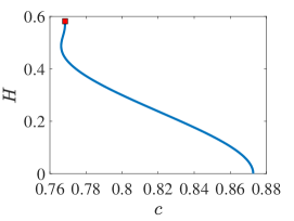
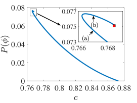
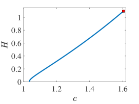
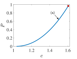
We begin by taking and . Figure 1 shows the wave height
| (24) |
and the momentum
| (25) |
from our numerical continuation of periodic and even solutions of (8) and (9). The result agrees, qualitatively, with [20, Figure 4] and others. We find that monotonically increases to , highlighted with the red square, for which (13) holds, whereas increases and then decreases, making one turning point. Also we find that the crest becomes sharper and the trough flatter as increases. The limiting solution must possess a cusp at the crest [9].
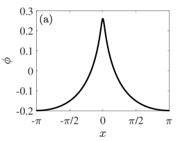
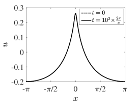
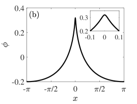
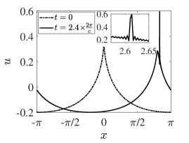
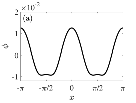
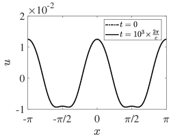
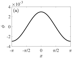
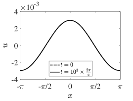
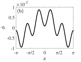
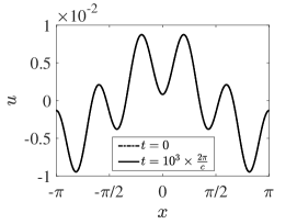
The left column of Figure 2 shows almost limiting waves. The inset is a close-up near the crest, emphasizing smoothness. The right column shows the profiles of (22), namely periodic traveling waves of (7) perturbed by uniformly distributed random noise of small amplitudes at (dash-dotted), and of the solutions of (7) at later instants of time (solid). Wave (a), prior to the turning point of , remains unchanged for time periods, after translation of the axis, implying orbital stability, whereas the inset reveals that wave (b), past the turning point, suffers from crest instability. Indeed, our numerical experiments point to transition from stability to instability at the turning point of . But there is numerical evidence [28] that waves (a) and (b) are (spectrally) modulationally unstable.
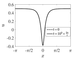
When and , Figure 3 shows and versus . Our numerical findings suggest that monotonically. Also . The solution branch discontinues once (14) holds, highlighted with the red square, though, because the solution would be physically unrealistic, for the capillary-gravity Whitham equation models water waves in the finite depth. Our numerical continuation works well past the limiting admissible solution, nevertheless. We find that the crest becomes wider and flatter, the trough narrower and more peaked, as increases. But all solutions must be smooth [8].
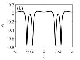
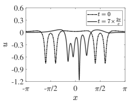
The left panel of Figure 4 shows an example wave. The right panel shows the profiles perturbed by small random noise at and of the solution of (7) after time periods, after translation of the axis. Our numerical experiments suggest orbital stability for all wave height. But there is numerical evidence of modulational instability when is large [3].
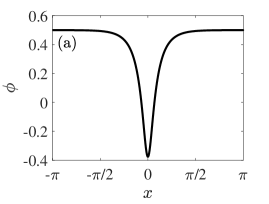
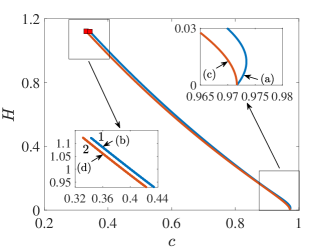
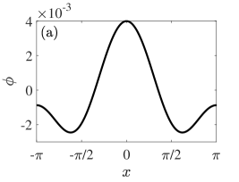
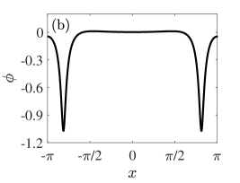
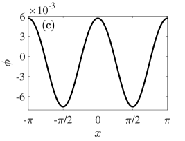
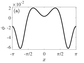
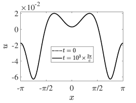
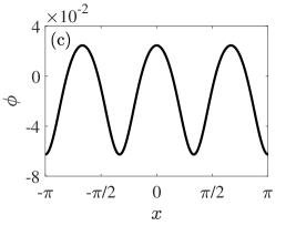
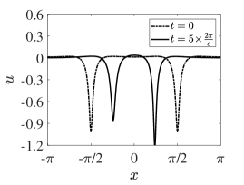
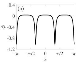
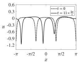
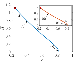
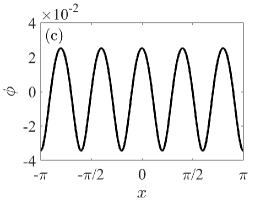
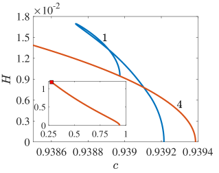
We turn the attention to (see (10)). There exists a two-parameter sheet of nontrivial, periodic and even solutions of (8) and (9) in the vicinity of and [8]. See also Section 2. Figure 5 shows versus for the and branches, all the way up to the limiting admissible solutions. There are no∥∥∥∥∥∥We observe a turning point of for greater wave height, but the solution is inadmissible. turning points of . The left column of Figure 6 shows waves in the and branches for small and large . The small height result agrees with [27, Figure 6].
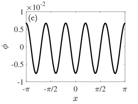
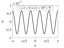
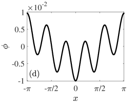
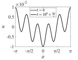
Observe ‘bimodal’ waves in the branch. Indeed, there cannot exist periodic and unimodal waves, whose profile monotonically decreases from a single crest to the trough over the period [8]. See also Section 2. For small wave height, the fundamental mode seems dominant, so that there is one crest over the period , but the fundamental and second modes are resonant, whereby a much smaller wave breaks up the trough into two. See the left panel of Figure 6(a). As increases, the effects of the second mode seem more pronounced, so that the wave separating the troughs becomes higher. See the left of Figure 6(b). Observe, to the contrary, periodic and unimodal waves in the branch. See the left of Figure 6(c,d). We find that the crests become wider and flatter, the troughs narrower and more peaked, as increases in the and branches. See the left of Figure 6(b,d).
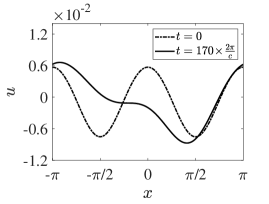
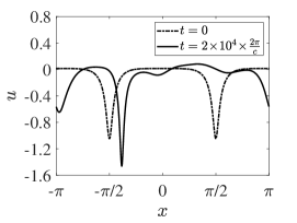
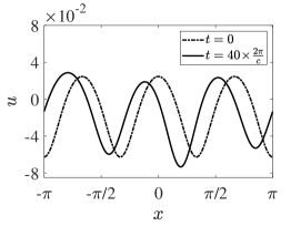
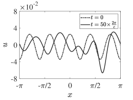
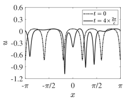
Our numerical experiments suggest orbital stability for the branch (see the right panels of Figure 6(a,b)) versus instability for (see the right of Figure 6(c,d)).
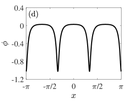
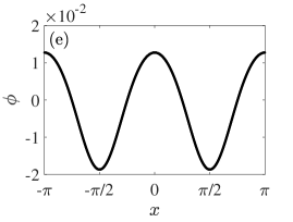
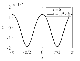
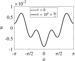
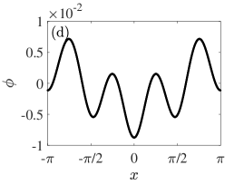
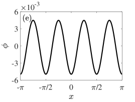
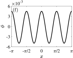
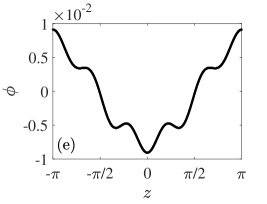
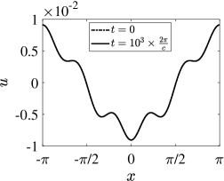
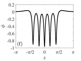
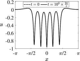
We take matters further to . See Figures 7, 8 and 9. The results for the and branches are similar to those when and . We pause to remark that in the branch, for small , a smaller wave breaks up the trough into two, and a much smaller wave breaks up the crest into two. See the left panel of Figure 8(a). As increases, the wave separating the crests becomes lower, transforming into one wide and flat crest, whereas the wave separating the troughs become higher (see the left of Figure 8(b)), whereby resembling those when and . Observe periodic and unimodal waves in the branch, orbitally stable for small versus unstable for large . See Figure 9(e,f).
When , to the contrary, we find and periodic unimodal waves in the and branches, respectively, corroborating a local bifurcation theorem (see [8], for instance). See also Section 2. We find that the crests become wider and flatter, the troughs narrower and more peaked, as increases. See the left column of Figure 11. Our numerical experiments (see the right of Figure 11) suggest orbital instability for the branch for large and for for all .
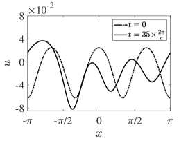
When , on the other hand, the left column of Figure 13 shows bimodal waves in the branch. The local bifurcation theorem [8] dictates periodic and unimodal waves, but we numerically find that they are not in the branch. For small , for wave (a), for instance, a smaller wave breaks up the trough into two over the half period. As increases, for wave (b), for instance, the troughs become narrower and more peaked. Our numerical experiments (see the right of Figures 13 and 14) suggest orbital stability for the branch for small versus instability for for large and for for all .
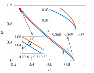
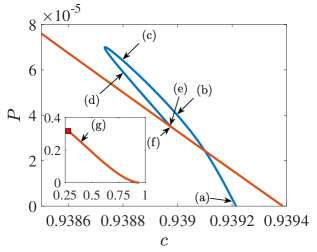
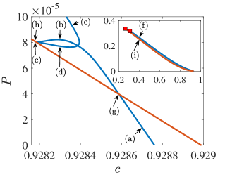
To proceed, when , the branch lies above and to the right of the branch at least for small (not shown), but as increases, increases more rapidly than , so that when , for instance, the branch crosses the branch. Figure 15 shows and versus in the and branches for all admissible solutions. The small height result agrees with [27, Figure 10(a)]. We find that in the branch, and turn to connect the branch, whereas in the branch, and monotonically increase to the limiting admissible solution, highlighted by the red square in the insets.
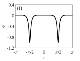
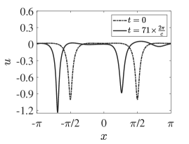
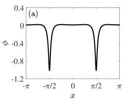
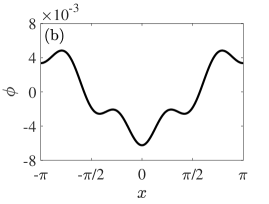
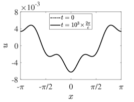
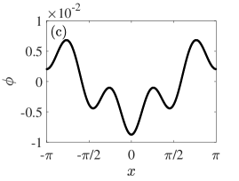
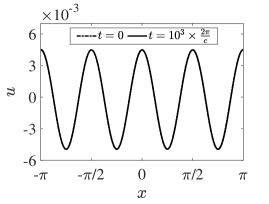
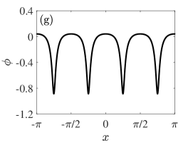
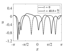
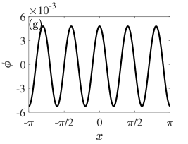
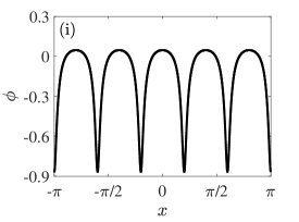
The left panels of Figures 16, 17 and 18 show several profiles along the and branches. In the branch, for small , wave (a), for instance, is periodic and unimodal. After the branch crosses the branch, on the other hand, wave (b), for instance, becomes bimodal, resembling those when and . Continuing along the branch, for waves (c) and (d), for instance, high frequency ripples of ride a carrier wave of . When the and branches almost connect, wave (e) in the branch and wave (f) for are almost the same. In the branch, wave (g), for instance, is periodic and unimodal.
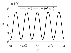
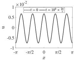
Our numerical experiments (see the right panels of Figures 16, 17 and 18) suggest orbital stability for the branch for all and for for small , versus instability for for large . Particularly, stability and instability do not change at the turning point of .
Last but not least, when , Figure 19 shows and versus for the and branches. The small height result agrees with [27, Figure 10(b)]. We find that the branch crosses and connects the branch, like when and , but it continues after connecting all the wave up to the limiting admissible solution. See the insets. The left panels of Figures 20, 21 and 22 show several profiles along the and branches. The results for the branch up to connecting and for are similar to those when and . In the branch, after it connects the branch at the point (c), the results are similar to those when and . See waves (d), (e) and (f). Our numerical experiments (see the right panels of Figures 20, 21 and 22) suggest orbital stability for the branch for all and for for small , versus instability for for large .
We emphasize orbital stability for the branch for all for all wave height throughout our numerical experiments.
5. Discussion
Here we employ efficient and highly accurate numerical methods for computing periodic traveling waves of (7) and experimenting with their (nonlinear) orbital stability and instability. Our findings suggest, among many others, stability whenever for the branch versus instability when for branches at least for large wave height. Currently under investigation is to take matters further to all to all , to classify the orbital stability and instability of all periodic traveling waves. It will be interesting to devise other numerical continuation methods, for instance, deflated continuation techniques [1, 4], for detecting disconnected solution branches and others. Also interesting will be to numerically investigate (spectral) modulational stability and instability of orbitally stable waves. Our methodology will be useful for exploring the nonlinear dynamics of modulationally unstable waves. Also it can help tackle the capillary-gravity wave problem and other nonlinear dispersive equations. Of course, it is of great importance to rigorously prove the numerical results.
Acknowledgement
The authors are grateful to Henrik Kalisch for helpful discussions. EGC acknowledges the hospitality of the Department of Mathematics at the University of Illinois at Urbana-Champaign where early stages of this work took place.
References
- [1] N. Boullé, E. G. Charalampidis, P. E. Farrell, and P. G. Kevrekidis, Deflation-based identification of nonlinear excitations of the three-dimensional Gross-Pitaevskii equation, Phys. Rev. A 102 (2020), no. 5, 053307, 8 pp.–53314. MR 4190003
- [2] John P. Boyd, Chebyshev and Fourier spectral methods, second ed., Dover Publications, Inc., Mineola, NY, 2001. MR 1874071
- [3] John D Carter and Morgan Rozman, Stability of periodic, traveling-wave solutions to the capillary Whitham equation, Fluids 4 (2019), no. 1, 58.
- [4] E. G. Charalampidis, N. Boullé, P. E. Farrell, and P. G. Kevrekidis, Bifurcation analysis of stationary solutions of two-dimensional coupled Gross-Pitaevskii equations using deflated continuation, Commun. Nonlinear Sci. Numer. Simul. 87 (2020), 105255, 24. MR 4101968
- [5] Evgueni Dinvay, Daulet Moldabayev, Denys Dutykh, and Henrik Kalisch, The Whitham equation with surface tension, Nonlinear Dynam. 88 (2017), no. 2, 1125–1138. MR 3628376
- [6] Eusebius Doedel, AUTO, http://indy.cs.concordia.ca/auto/.
- [7] Eusebius Doedel and Laurette S. Tuckerman (eds.), Numerical methods for bifurcation problems and large-scale dynamical systems, The IMA Volumes in Mathematics and its Applications, vol. 119, Springer-Verlag, New York, 2000. MR 1768354
- [8] Mats Ehrnström, Mathew A. Johnson, Ola I. H. Maehlen, and Filippo Remonato, On the Bifurcation Diagram of the Capillary–Gravity Whitham Equation, Water Waves 1 (2019), no. 2, 275–313. MR 4176870
- [9] Mats Ehrnström and Erik Wahlén, On Whitham’s conjecture of a highest cusped wave for a nonlocal dispersive equation, Ann. Inst. H. Poincaré Anal. Non Linéaire 36 (2019), no. 6, 1603–1637. MR 4002168
- [10] David Gottlieb and Steven A. Orszag, Numerical analysis of spectral methods: theory and applications, Society for Industrial and Applied Mathematics, Philadelphia, Pa., 1977, CBMS-NSF Regional Conference Series in Applied Mathematics, No. 26. MR 0520152
- [11] E. Hairer, S. P. Nø rsett, and G. Wanner, Solving ordinary differential equations. I, second ed., Springer Series in Computational Mathematics, vol. 8, Springer-Verlag, Berlin, 1993, Nonstiff problems. MR 1227985
- [12] E. Hairer and G. Wanner, Solving ordinary differential equations. II, second ed., Springer Series in Computational Mathematics, vol. 14, Springer-Verlag, Berlin, 1996, Stiff and differential-algebraic problems. MR 1439506
- [13] Vera Mikyoung Hur, Wave breaking in the Whitham equation, Adv. Math. 317 (2017), 410–437. MR 3682673
- [14] by same author, Shallow water models with constant vorticity, Eur. J. Mech. B Fluids 73 (2019), 170–179. MR 3907481
- [15] Vera Mikyoung Hur and Mathew A. Johnson, Modulational instability in the Whitham equation for water waves, Stud. Appl. Math. 134 (2015), no. 1, 120–143. MR 3298879
- [16] by same author, Modulational instability in the Whitham equation with surface tension and vorticity, Nonlinear Anal. 129 (2015), 104–118. MR 3414922
- [17] by same author, Stability of periodic traveling waves for nonlinear dispersive equations, SIAM J. Math. Anal. 47 (2015), no. 5, 3528–3554. MR 3397429
- [18] Vera Mikyoung Hur and Ashish Kumar Pandey, Modulational instability in the full-dispersion Camassa-Holm equation, Proc. A. 473 (2017), no. 2203, 20171053, 18. MR 3685469
- [19] by same author, Modulational instability in a full-dispersion shallow water model, Stud. Appl. Math. 142 (2019), no. 1, 3–47. MR 3897262
- [20] Henrik Kalisch, Daulet Moldabayev, and Olivier Verdier, A numerical study of nonlinear dispersive wave models with SpecTraVVave, Electron. J. Differential Equations (2017), Paper No. 62, 23. MR 3625942
- [21] Henrik Kalisch and Didier Pilod, On the local well-posedness for a full-dispersion Boussinesq system with surface tension, Proc. Amer. Math. Soc. 147 (2019), no. 6, 2545–2559. MR 3951431
- [22] Aly-Khan Kassam and Lloyd N. Trefethen, Fourth-order time-stepping for stiff PDEs, SIAM J. Sci. Comput. 26 (2005), no. 4, 1214–1233. MR 2143482
- [23] C. T. Kelley, Solving nonlinear equations with Newton’s method, Fundamentals of Algorithms, vol. 1, Society for Industrial and Applied Mathematics (SIAM), Philadelphia, PA, 2003. MR 1998383
- [24] Felipe Linares, Didier Pilod, and Jean-Claude Saut, Remarks on the orbital stability of ground state solutions of fKdV and related equations, Adv. Differential Equations 20 (2015), no. 9-10, 835–858. MR 3360393
- [25] Daulet Moldabayev, Henrik Kalisch, and Denys Dutykh, The Whitham equation as a model for surface water waves, Phys. D 309 (2015), 99–107. MR 3390078
- [26] Ashish Kumar Pandey, The effects of surface tension on modulational instability in full-dispersion water-wave models, Eur. J. Mech. B Fluids 77 (2019), 177–182. MR 3952644
- [27] Filippo Remonato and Henrik Kalisch, Numerical bifurcation for the capillary Whitham equation, Phys. D 343 (2017), 51–62. MR 3606200
- [28] Nathan Sanford, Keri Kodama, John D. Carter, and Henrik Kalisch, Stability of traveling wave solutions to the Whitham equation, Phys. Lett. A 378 (2014), no. 30-31, 2100–2107. MR 3226084
- [29] J. Sullivan, E. G. Charalampidis, J. Cuevas-Maraver, P. G. Kevrekidis, and N. I. Karachalios, Kuznetsov–Ma breather-like solutions in the Salerno model, The European Physical Journal Plus 135 (2020), no. 7, 607.
- [30] G. B. Whitham, Variational methods and applications to water waves, Proceedings of the Royal Society of London. Series A, Mathematical and Physical Sciences 299 (1967), no. 1456, 6–25.
- [31] G. B. Whitham, Linear and nonlinear waves, Pure and Applied Mathematics (New York), John Wiley & Sons, Inc., New York, 1999, Reprint of the 1974 original, A Wiley-Interscience Publication. MR 1699025