A Scalable Two Stage Approach to Computing Optimal Decision Sets

Abstract

Machine learning (ML) is ubiquitous in modern life. Since it is being deployed in technologies that affect our privacy and safety, it is often crucial to understand the reasoning behind its decisions, warranting the need for explainable AI. Rule-based models, such as decision trees, decision lists, and decision sets, are conventionally deemed to be the most interpretable. Recent work uses propositional satisfiability (SAT) solving (and its optimization variants) to generate minimum-size decision sets. Motivated by limited practical scalability of these earlier methods, this paper proposes a novel approach to learn minimum-size decision sets by enumerating individual rules of the target decision set independently of each other, and then solving a set cover problem to select a subset of rules. The approach makes use of modern maximum satisfiability and integer linear programming technologies. Experiments on a wide range of publicly available datasets demonstrate the advantage of the new approach over the state of the art in SAT-based decision set learning.

1 Introduction

Rapid advances in artificial intelligence and, in particular, in machine learning (ML), have influenced all aspects of human lives. Given the practical achievements and the overall success of modern approaches to ML (LeCun, Bengio, and Hinton 2015; Jordan and Mitchell 2015; Mnih et al. 2015; ACM 2018), one can argue that it will prevail as a generic computing paradigm and it will find an ever growing range of practical applications. Unfortunately, the most widely used ML models are opaque, which makes it hard for a human decision-maker to comprehend the outcomes of such models. This motivated efforts on validating the operation of ML models (Ruan, Huang, and Kwiatkowska 2018; Katz et al. 2017) but also on devising approaches to explainable artificial intelligence (XAI) (Ribeiro, Singh, and Guestrin 2016; Lundberg and Lee 2017; Monroe 2018).

One of the major lines of work in XAI is devoted to training logic-based models, e.g. decision trees (Bessiere, Hebrard, and O’Sullivan 2009; Narodytska et al. 2018; Hu, Rudin, and Seltzer 2019; Aglin, Nijssen, and Schaus 2020), decision lists (Angelino et al. 2017; Rudin and Ertekin 2018) or decision sets (Lakkaraju, Bach, and Leskovec 2016; Ignatiev et al. 2018; Malioutov and Meel 2018; Ghosh and Meel 2019; Yu et al. 2020), where concise explanations can be obtained directly from the model. This paper focuses on the decision set (DS) model, which comprises an unordered set of if-then rules.

One of the advantages of decision sets over other rule-based models is that rule independence makes it straightforward to explain a prediction: a user can pick any rule that “fires” the prediction and the rule itself serves as the explanation. As a result, generation of minimum-size decision sets is of great interest. Recent work proposed SAT-based methods for generating minimum-size decision sets by solving a sequence of problems that determine whether a decision set of size $K$ exists, with $K$ being the number of rules (Ignatiev et al. 2018) or the number of literals (Yu et al. 2020) s.t. the decision set agrees with the training data. Unfortunately, scalability of both approaches is limited due to the large size of the propositional encoding.

Motivated by this limitation, our work proposes a novel approach that splits the DS generation problem into two parts: (1) exhaustive rule enumeration and (2) computing a subset of rules agreeing with the training data. In general, this novel approach enables a significantly more compact propositional encoding, which makes it scalable for problem instances that are out of reach for the state of the art. The proposed approach is inspired by the standard setup used in two-level logic minimization (Quine 1952, 1955; McCluskey 1956). While the first part can be done using enumeration of maximum satisfiability (MaxSAT) solutions, the second part is reduced to the set cover problem, for which integer linear programming (ILP) is effective. Experiments on a wide range of datasets indicate that this approach outperforms the state of the art. The remainder of this paper presents these developments in detail.

2 Preliminaries

Satisfiability and Maximum Satisfiability.

We use the standard definitions for propositional satisfiability (SAT) and maximum satisfiability (MaxSAT) solving (Biere et al. 2009). SAT and MaxSAT admit Boolean variables. A literal over Boolean variable $x$ is either the variable $x$ itself or its negation $\neg{x}$. (Given a constant parameter $\sigma\in\{0,1\}$, we use notation $x^{\sigma}$ to represent literal $x$ if $\sigma=1$, and to represent literal $\neg{x}$ if $\sigma=0$.) A clause is a disjunction of literals. A term is a conjunction of literals. A propositional formula is said to be in conjunctive normal form (CNF) or disjunctive normal form (DNF) if it is a conjunction of clauses or disjunction of terms, respectively. Whenever convenient, clauses and terms are treated as sets of literals. Formulas written as sets of sets of literals (either in CNF or DNF) are described as clausal.

We will make use of partial maximum satisfiability (Partial MaxSAT) (Biere et al. 2009, Chapter 19), which can be formulated as follows. A partial CNF formula can be seen as a conjunction of hard clauses ${\mathcal{H}}$ (which must be satisfied) and soft clauses ${\mathcal{S}}$ (which represent a preference to satisfy those clauses). The Partial MaxSAT problem consists in finding an assignment that satisfies all the hard clauses and maximizes the total number of satisfied soft clauses.

Classification Problems and Decision Sets.

We follow the notation used in earlier work (Bessiere, Hebrard, and O’Sullivan 2009; Lakkaraju, Bach, and Leskovec 2016; Ignatiev et al. 2018; Yu et al. 2020). Consider a set of features ${\mathcal{F}}=\{1,\ldots,K\}$. The domain of possible values for feature $r\in[K]$ is $D_{r}$. The complete space of feature values (or feature space (Han, Kamber, and Pei 2012)) is $\mathbb{F}\triangleq\prod_{r=1}^{K}D_{r}$. The vector $\mathbf{f}=(f_{1},\ldots,f_{K})$ of $K$ variables $f_{r}\in D_{r}$ refers to a point in $\mathbb{F}$. Concrete (constant) points in $\mathbb{F}$ are denoted by $\mathbf{v}=(v_{1},\ldots,v_{K})$, with $v_{r}\in D_{r}$. For simplicity, all the features are assumed to be binary, i.e. $D_{r}=\{0,1\},\forall r\in[K]$; categorical and ordinal features can be mapped to binary features using standard techniques (Pedregosa et al. 2011). Therefore, whenever convenient, a Boolean literal on a feature $r$ can be represented as $f_{r}$ (or $\neg{f_{r}}$, resp.), denoting that feature $f_{r}$ takes value 1 (value 0, resp.).

Consider a standard classification scenario with training data ${\mathcal{E}}=\{e_{1},\ldots,e_{M}\}$. A data instance (or example) $e_{i}\in{\mathcal{E}}$ is a pair $(\mathbf{v}_{i},c_{i})$ where $\mathbf{v}_{i}\in\mathbb{F}$ is a vector of feature values and $c_{i}\in{\mathcal{C}}$ is a class. An example $e_{i}$ can be seen as associating a vector of feature values $\mathbf{v}_{i}$ with a class $c_{i}\in{\mathcal{C}}$. This work focuses on binary classification problems, i.e. ${\mathcal{C}}=\{\ominus,\oplus\}$ but the proposed ideas are easily extendable to the case of multiple classes. Given example $e_{i}=(\mathbf{v}_{i},c_{i})\in{\mathcal{E}}$ and the $r^{\text{th}}$ component $v_{ir}$ of $\mathbf{v}_{i}$, literal $f_{r}^{1-v_{ir}}$ is said to discriminate $e_{i}$ because $f_{r}^{1-v_{ir}}\triangleq\neg{v_{ir}}$, i.e. $f_{r}^{1-v_{ir}}$ falsifies example $e_{i}$ when it is considered as a conjunction of feature literals. The concept of example discrimination can be extended to terms.

Examples $e_{i},e_{j}\in{\mathcal{E}}$ associating the same set of feature values with the opposite classes are referred to as overlapping. We assume wlog. that the training data ${\mathcal{E}}$ is perfectly classifiable, i.e. ${\mathcal{E}}$ partially defines a Boolean function $\phi:\mathbb{F}\rightarrow{\mathcal{C}}$ — in other words, there are no overlapping examples in ${\mathcal{E}}$. Otherwise, either $e_{i}$ or $e_{j}$ can be removed from dataset ${\mathcal{E}}$, incurring an error of 1. In general, repeated “collisions” can be resolved by taking the majority vote, which results in highest possible accuracy on training data.

The objective of classification in ML is to devise a function $\hat{\phi}$ that matches the actual function $\phi$ on the training data ${\mathcal{E}}$ and generalizes suitably well on unseen test data (Fürnkranz, Gamberger, and Lavrac 2012; Han, Kamber, and Pei 2012; Mitchell 1997; Quinlan 1993). In many settings, function $\hat{\phi}$ is not required to match $\phi$ on the complete set of examples ${\mathcal{E}}$ and instead an accuracy measure is considered. Furthermore, in classification problems one conventionally has to optimize with respect to (1) the complexity of $\hat{\phi}$, (2) the accuracy of the learnt function (to make it match the actual function $\phi$ on a maximum number of examples), or (3) both. As this paper assumes that the training data does not have overlapping instances, we aim solely at minimizing the representation size of the target ML models.

This paper focuses on learning representations of $\hat{\phi}$ corresponding to decision sets (DS) (Lakkaraju, Bach, and Leskovec 2016; Ignatiev et al. 2018; Malioutov and Meel 2018; Ghosh and Meel 2019; Yu et al. 2020). A decision set is an unordered set of rules. Each rule $\pi$ is from the set ${\mathcal{R}}=\prod_{r=1}^{K}\{f_{r},\neg f_{r},\mathfrak{u}\}$, where $\mathfrak{u}$ represents a don’t care value. For each example $e\in{\mathcal{E}}$, a rule of the form $\pi\Rightarrow c$, $\pi\in{\mathcal{R}}$, $c\in{\mathcal{C}}$ is interpreted as “if the feature values of example $e$ agree with $\pi$ then the rule predicts that example $e$ has class $c$”. Hereinafter, we will be dealing with learning minimum-size decision sets, with the size measure being either the number of rules in the decision set or the total number of literals in it (sometimes referred to as total size). Note that because rules in decision sets are unordered, some rules may overlap, i.e. multiple rules $\pi_{i}\in{\mathcal{R}}$ may agree with some instance of the feature space $\mathbb{F}$. It may also happen that none of the rules of a decision set apply to some instances of $\mathbb{F}$.

Example 1.

Consider the following dataset of four data instances representing the “to date or not to date?” example by Domingos (2015):

#	Day	Venue	Weather	TV Show	Date?
$e_{1}$	Weekday	Dinner	Warm	Bad	No
$e_{2}$	Weekend	Club	Warm	Bad	Yes
$e_{3}$	Weekend	Club	Warm	Bad	Yes
$e_{4}$	Weekend	Club	Cold	Good	No

This data serves to predict whether a friend accepts an invitation to go out for a date given various circumstances. An example of a valid decision set for this data is the following:

$$\begin{array}[]{ll}\textbf{IF }\color[rgb]{0.125,0.2890625,0.53125}\text{ TV Show}=\text{Good}&\textbf{THEN }\color[rgb]{0.64453125,0,0}\text{ Date}=\text{No}\\ \textbf{IF }\color[rgb]{0.125,0.2890625,0.53125}\text{ Day}=\text{Weekday}&\textbf{THEN }\color[rgb]{0.64453125,0,0}\text{ Date}=\text{No}\\ \textbf{IF }\color[rgb]{0.125,0.2890625,0.53125}\text{ TV Show}=\text{Bad }\bm{\land}\text{ Day}=\text{Weekend}&\textbf{THEN }\color[rgb]{0.3046875,0.60546875,0.0234375}\text{ Date}=\text{Yes}\\ \end{array}$$

This DS has 3 rules and a total size of 7 (1 for each literal on the left and right, or alternatively, 1 for each literal on the left and 1 for each rule). It does not exhibit rule overlap for examples in $\mathbb{F}$ while the following decision set does:

$$\begin{array}[]{ll}\textbf{IF }\color[rgb]{0.125,0.2890625,0.53125}\text{ TV Show}=\text{Good}&\textbf{THEN }\color[rgb]{0.64453125,0,0}\text{ Date}=\text{No}\\ \textbf{IF }\color[rgb]{0.125,0.2890625,0.53125}\text{ Day}=\text{Weekday}&\textbf{THEN }\color[rgb]{0.64453125,0,0}\text{ Date}=\text{No}\\ \textbf{IF }\color[rgb]{0.125,0.2890625,0.53125}\text{ Weather}=\text{Warm }\bm{\land}\text{ Day}=\text{Weekend}&\textbf{THEN }\color[rgb]{0.3046875,0.60546875,0.0234375}\text{ Date}=\text{Yes}\\ \end{array}$$

Here, the first and third rules overlap for all examples with feature values $\textit{Weather}=\textit{Warm}$ and $\textit{TV Show}=\textit{Good}$. ∎

3 Related Work

Rule-based ML models can be traced back to around the 70s and 80s (Michalski 1969; Shwayder 1975; Hyafil and Rivest 1976; Breiman et al. 1984; Quinlan 1986; Rivest 1987). To our best knowledge, decision sets first appear as an unordered variant of decision lists (Rivest 1987; Clark and Niblett 1989) in (Clark and Boswell 1991). The use of logic and optimization for synthesizing a disjunction of rules matching a given training dataset was first tried in (Kamath et al. 1992). Recently, (Lakkaraju, Bach, and Leskovec 2016) argued that decision sets are more interpretable than decision trees and decision lists.

Our work builds on (Ignatiev et al. 2018; Yu et al. 2020) where SAT-based models were proposed for training decision sets of smallest size. The method of (Ignatiev et al. 2018) minimized the number of rules in perfect decision sets, i.e. those that agree perfectly with the training data, which is assumed to be consistent; it was also shown to significantly outperform the smooth local search approach of (Lakkaraju, Bach, and Leskovec 2016). Rule minimization was then followed by minimization of the total number of literals used in the decision set, which resulted in a lexicographic approach to the minimization problem. In contrast, (Yu et al. 2020) focused on minimizing the total number of literals in the target DS. This work showed that minimizing the number of rules is more scalable for solving the perfect decision set problem since the optimization measure, i.e. the number of rules, is more coarse-grained. However, minimizing the total number of literals was shown to produce significantly smaller and, thus, more interpretable target decision sets. Furthermore, they showed that sparse decision sets (minimizing either the number of literals or the number or rules) provide a user with yet another way to produce a succinct classifier representation, by trading off its accuracy for smaller size. Sparse decision sets were also considered in (Malioutov and Meel 2018; Ghosh and Meel 2019) where the authors proposed a MaxSAT model for representing one target class of the training data. ILP was also applied to compute a variant of sparse decision sets (Dash, Günlük, and Wei 2018). As was shown in (Yu et al. 2020), sparse decision sets, although are much easier to compute, achieve lower test accuracy compared to perfect decision sets. As a result, the focus of this work is solely on improving scalability of computing perfect decision sets, i.e. sparse models are excluded from consideration.

4 Decision Sets by Rule Enumeration

Similar to the recent logic-based approaches to learning decision sets (Ignatiev et al. 2018; Malioutov and Meel 2018; Ghosh and Meel 2019), our approach builds on state-of-the-art SAT and MaxSAT technology. These prior works consider a SAT or MaxSAT model that determines whether there exists a decision set of size $N$ given training data ${\mathcal{E}}$ with $|{\mathcal{E}}|=M$ examples. The problem is solved by iteratively varying size $N$ and making either a series of SAT calls or one MaxSAT call. The main limitation of prior work is the encoding formula size, which is ${\mathcal{O}}(N\times M\times K)$, where $N$ is the target size of decision set (which is determined either as the number of rules (Ignatiev et al. 2018) or as the total number of literals (Yu et al. 2020)), $M$ is the number of training data instances and $K$ is the number of features in the training data. This limitation significantly impairs scalability of these approaches and hence restricts their practical applicability.

In contrast to the aforementioned works, the approach detailed below does not aim at devising a decision set in one step and instead consists of two phases. The first phase sequentially enumerates all individual minimal rules given an input dataset. The second phase computes a minimum-size subset of rules (either in terms of the number of rules or the total number of literals in use) that covers all the training data instances. This way the approach trades off large encoding size and thus potentially hard SAT oracle calls for computing a complete decision set with a (much) larger number of simpler oracle calls, each computing an individual rule, followed by solving the set cover problem. This algorithmic setup is, in a sense, inspired by the effectiveness of the standard clausal formula minimization approach (Quine 1952, 1955; McCluskey 1956; Brayton et al. 1984; Espresso ).

4.1 Decision Sets as DNF Formulas

First, recall that we consider binary classification, i.e. ${\mathcal{C}}=\{\ominus,\oplus\}$ but the ideas of this section can be easily adapted to multi-class problems, e.g. by using one-hot encoding (Pedregosa et al. 2011). Next, let us split the set of training examples ${\mathcal{E}}$ into the sets of examples ${\mathcal{E}}_{\oplus}$ and ${\mathcal{E}}_{\ominus}$ for the respective classes s.t. ${\mathcal{E}}={\mathcal{E}}_{\oplus}\cup{\mathcal{E}}_{\ominus}$ and ${\mathcal{E}}_{\oplus}\cap{\mathcal{E}}_{\ominus}=\emptyset$.

Recall that a decision set is an unordered set of if-then rules $\pi\Rightarrow c$, each associating a set of literals $\pi\in{\mathcal{R}}$, ${\mathcal{R}}=\prod_{r=1}^{K}\{f_{r},\neg f_{r},\mathfrak{u}\}$, over the feature-values present in rule $\pi$ with the corresponding class $c\in\{\ominus,\oplus\}$. Following (Ignatiev et al. 2018), observe that each set of literals $\pi$ in the rule forms a term and so every class $c_{i}\in\{\ominus,\oplus\}$ in a decision set can be represented logically as a disjunction of terms, each term representing a conjunction of literals in $\pi$.

Example 2.

Consider our example dataset shown in Example 1. Assume that features Day, Venue, Weather, and TV Show are represented with Boolean variables $f_{1}$, $f_{2}$, $f_{3}$, and $f_{4}$, respectively. Observe that all the features $f_{r}$, $r\in[4]$, in the example are binary, and thus each value for feature $f_{r}$ can be represented either as literal $f_{r}$ or literal $\neg{f_{r}}$. Let us map the original feature values to $\{0,1\}$ such that the alphabetically-first value is mapped to $0$ while the other is mapped to $1$. The classes No and Yes are mapped to $\ominus$ and $\oplus$, respectively. As a result, our dataset becomes

$f_{1}$	$f_{2}$	$f_{3}$	$f_{4}$	$c$
0	1	1	0	$\ominus$
1	0	1	0	$\oplus$
1	0	1	0	$\oplus$
1	0	0	1	$\ominus$

Using this binary dataset and the first decision set from Example 1 the classes $c=\ominus$ and $c=\oplus$ are represented as the DNF formulas ${\phi}_{\ominus}\triangleq(f_{4})\lor(\neg{f_{1}})$ and ${\phi}_{\oplus}\triangleq(\neg{f_{4}}\land f_{1})$ ∎

In this work, we follow (Ignatiev et al. 2018; Yu et al. 2020) and compute minimum-size decision sets in the form of disjunctive representations ${\phi}_{\ominus}$ and ${\phi}_{\oplus}$ of classes $\ominus$ and $\oplus$. Even though it is simpler to construct rules for one class when there are only two classes (Malioutov and Meel 2018; Ghosh and Meel 2019), computing both ${\phi}_{\ominus}$ and ${\phi}_{\oplus}$ achieves better interpretability. Specifically, if both classes are explicitly represented, it is relatively easy to extract explicit and succinct explanations for any class, but this is not the case when only one class is computed. This approach also immediately extends to problems with three or more classes.

Without loss of generality, we focus on computing a disjunctive representation ${\phi}_{\oplus}$ for the class $c=\oplus$. The same reasoning can be applied to compute ${\phi}_{\ominus}$. The target DNF ${\phi}_{\oplus}$ must be consistent with the training data, i.e. every term $\pi\in{\phi}_{\oplus}$ must (1) agree with at least one example $e_{i}\in{\mathcal{E}}_{\oplus}$ and (2) discriminate all examples $e_{j}\in{\mathcal{E}}_{\ominus}$. Furthermore, each term $\pi\in{\phi}_{\oplus}$ must be irreducible, meaning that any subterm $\pi^{\prime}\subsetneq\pi$ does not fulfill one of the two conditions above.

4.2 Learning Rules

This section describes the first phase of the proposed approach, namely, how a term $\pi$ satisfying both of the conditions above can be obtained separately of the other terms. Every term is computed as a MaxSAT solution to a partial CNF formula

$$\psi\triangleq{\mathcal{H}}\land{\mathcal{S}}$$ (1)

with ${\mathcal{H}}$ and ${\mathcal{S}}$ being the hard and soft parts, described below.

Consider two sets of Boolean variables $P$ and $N$, $|P|=|N|=K$. For every feature $f_{r}$, $r\in[K]$, define variables $p_{r}\in P$ and $n_{r}\in N$. The idea is inspired by the dual-rail encoding (DRE) of propositional formulas (Bryant et al. 1987), e.g. studied in the context of logic minimization (Manquinho et al. 1997; Jabbour et al. 2014). Variables $p_{r}$ and $n_{r}$ are referred to as dual-rail variables. We assume that $p_{r}=1$ iff $f_{r}=1$ while $n_{r}=1$ iff $f_{r}=0$. Moreover, for every feature $f_{r}$, $r\in[K]$, a hard clause is added to ${\mathcal{H}}$ to forbid the feature taking two values at once:

$$\forall_{r\in[K]}\;\;(\neg{p_{r}}\lor\neg{n_{r}})$$ (2)

The other combinations of values for $p_{r}$ and $n_{r}$ encode the fact that feature $r$ occurs in the target term $\pi$ positively, negatively, or does not occur at all (when $p_{r}=n_{r}=0$).

The set of soft clauses ${\mathcal{S}}$ represents a preference to discard the features from a target term $\pi$ and thus contains a pair of soft unit clauses expressing that preference:

$${\mathcal{S}}\triangleq\left\{(\neg{p_{r}}),(\neg{n_{r}})\;|\;r\in[K]\right\}$$ (3)

By construction of ${\mathcal{S}}$ and given a MaxSAT solution for (1), the target term $\pi$ is composed of all features $f_{r}$, for which one of the dual-rail variables (either $p_{r}$ or $n_{r}$) is assigned to 1 by the solution, i.e. the corresponding soft clauses are falsified.

Discrimination Constraints.

Every example $e_{j}=(\mathbf{v}_{j},\ominus)$ from ${\mathcal{E}}_{\ominus}$ must be discriminated. This can be enforced by using a clause $(\bigvee_{r\in[K]}{f_{r}^{1-v_{jr}}})$, where constant $v_{jr}$ is the value of the $r^{\text{th}}$ feature in example $e_{j}$. To represent this in the dual-rail formulation, we add the following hard clauses to ${\mathcal{H}}$:

$$\forall_{j\in[|{\mathcal{E}}_{\ominus}|]}\;\;\bigvee_{r\in[K]}{\delta_{jr}},$$ (4)

where $\delta_{jr}$ is to be replaced by dual-rail variable $p_{r}$ if $v_{jr}=0$ and replaced by the opposite dual-rail variable $n_{r}$ if $v_{jr}=1$.

Example 3.

Consider instance $e_{1}=(f_{1}=0,f_{2}=1,f_{3}=1,f_{4}=0)\in{\mathcal{E}}_{\ominus}$ of the running example. To discriminate it, we add a hard clause $(p_{1}\lor n_{2}\lor n_{3}\lor p_{4})$. Indeed, to satisfy this clause, we have to pick one of the literals discriminating example $e_{1}$, e.g. if $p_{1}=1$ then literal $f_{1}$ occurs in term $\pi$, which discriminates instance $e_{1}$. ∎

Coverage Constraints.

To enforce that every term $\pi$ covers at least one training instance of ${\mathcal{E}}_{\oplus}$, we can use similar reasoning. Observe that a term $\pi\in{\mathcal{R}}$ covers instance $e_{i}=(\mathbf{v}_{i},c_{i})\in{\mathcal{E}}_{\oplus}$ iff none of its literals discriminates $e_{i}$, i.e. $f_{r}^{1-v_{jr}}\not\in\pi$ for any $r\in[K]$. For each example $e_{i}=(\mathbf{v}_{i},c_{i})\in{\mathcal{E}}_{\oplus}$, we introduce an auxiliary variable $t_{i}$ defined by:

$$t_{i}\leftrightarrow\neg(\bigvee_{r=1}^{K}{\delta_{ir}}),$$ (5)

where $\delta_{ir}$ is to be replaced by dual-rail variable $p_{r}$ if $v_{ir}=0$ and replaced by the opposite dual-rail variable $n_{r}$ if $v_{ir}=1$. Now, variable $t_{i}$ is true iff term $\pi$ covers example $e_{i}$.

Example 4.

Consider instance $e_{2}=(f_{1}=1,f_{2}=0,f_{3}=1,f_{4}=0)\in{\mathcal{E}}_{\oplus}$ of the running example. Introduce variable $t_{2}\leftrightarrow\neg(n_{1}\lor p_{2}\lor n_{3}\lor p_{4})$ as shown above. If $t_{2}=1$, the literals in the target term $\pi$ cannot discriminate example $e_{2}$. ∎

Once auxiliary variables $t_{i}$ are introduced for each example $e_{i}\in{\mathcal{E}}_{\oplus}$, the hard clause

$$\bigvee\nolimits_{i\in[|{\mathcal{E}}_{\oplus}|]}t_{i}$$ (6)

can be added ${\mathcal{H}}$ to ensure that any term $\pi$ agrees with at least one of the training data instances.

The overall partial MaxSAT model (1) comprises hard clauses (2), (4), (5), (6) and also soft clauses (3). The number of variables used in the encoding is ${\mathcal{O}}(K+M)$ while the number of clauses is ${\mathcal{O}}(K\times M)$. Recall that earlier works proposed encoding with ${\mathcal{O}}(N\times M\times K)$ variables and clauses, which in some situations makes it hard (or infeasible) to prove optimality of large decision sets.

Example 5.

Consider our aim at computing rules for class $\oplus$ in the running example. By applying the DRE, one obtains the formula $\psi={\mathcal{H}}\land{\mathcal{S}}$ where

$${\mathcal{H}}=\left\{\begin{array}[]{c}(\neg{p_{1}}\lor\neg{n_{1}})\land(\neg{p_{2}}\lor\neg{n_{2}})\land\\ (\neg{p_{3}}\lor\neg{n_{3}})\land(\neg{p_{4}}\lor\neg{n_{4}})\land\\ \\ (p_{1}\lor n_{2}\lor n_{3}\lor p_{4})\land\\ (n_{1}\lor p_{2}\lor p_{3}\lor n_{4})\land\\ \\ \left[t_{2}\leftrightarrow\neg(n_{1}\lor p_{2}\lor n_{3}\lor p_{4})\right]\land\\ \left[t_{3}\leftrightarrow\neg(n_{1}\lor p_{2}\lor n_{3}\lor p_{4})\right]\land\\ (t_{2}\lor t_{3})\end{array}\right\}$$

and

$${\mathcal{S}}=\left\{\begin{array}[]{c}(\neg{p_{1}})\land(\neg{n_{1}})\land(\neg{p_{2}})\land(\neg{n_{2}})\land\\ (\neg{p_{3}})\land(\neg{n_{3}})\land(\neg{p_{4}})\land(\neg{n_{4}})\\ \end{array}\right\}$$

∎

Any assignment satisfying the hard clauses ${\mathcal{H}}$ of the dual-rail MaxSAT formula (1) constructed above defines a term $\pi$ that discriminates all examples of ${\mathcal{E}}_{\ominus}$ and covers at least one example of ${\mathcal{E}}_{\oplus}$; soft clauses ${\mathcal{S}}$ ensure minimality of terms $\pi$. More importantly, one can exhaustively enumerate all solutions of (1) to compute the set of all such terms (i.e. one can use the standard trick of adding a hard clause blocking the previous solution and ask for a new one until no more solutions can be found). Let us refer to this set of terms as ${\mathcal{T}}_{\oplus}$. Finally, we claim that as soon as exhaustive solution enumeration for formula (1) is finished, the set of terms ${\mathcal{T}}_{\oplus}$ covers every example $e_{i}\in{\mathcal{E}}_{\oplus}$. The rationale is that if sets ${\mathcal{E}}_{\oplus}$ and ${\mathcal{E}}_{\ominus}$ do not overlap then for any example $e_{i}\in{\mathcal{E}}_{\oplus}$ there is a way to cover it by a term $\pi$ s.t. all examples of ${\mathcal{E}}_{\ominus}$ are discriminated by $\pi$. This means that, by construction of (1), for every variable $t_{i}$, the hard part ${\mathcal{H}}$ of the formula has a satisfying assignment assigning $t_{i}=1$. (Recall that we assume training data to be perfectly classifiable.)

Example 6.

Consider our running example. Observe that a valid solution for formula $\psi$ above is $\{p_{1},n_{4}\}$ from which we can extract a term $\pi=(f_{1}\land\neg{f_{4}})$ for the target class $c=\oplus$. The term $\pi$ is added to ${\mathcal{T}}_{\oplus}$. Observe that $\pi$ covers both examples $e_{2}$ and $e_{3}$ and discriminates examples $e_{1}$ and $e_{4}$ from class $\ominus$. ∎

4.3 Smallest Rule Cover

Once the set ${\mathcal{T}}_{\oplus}$ of all terms for class $c=\oplus$ is obtained, the next step of the approach is to compute a smallest size cover ${\phi}_{\oplus}$ of the training examples ${\mathcal{E}}_{\oplus}$. Concretely, the problem is to select the smallest size subset ${\phi}_{\oplus}$ of ${\mathcal{T}}_{\oplus}$ that covers all the training examples. The size can be the either the number of terms used or the total number of literals used in ${\phi}_{\oplus}$. Therefore, the problem to solve is essentially the set cover problem (Karp 1972). Assume that $|{\mathcal{T}}_{\oplus}|=L$ and create a Boolean variable $b_{j}$ for every term $\pi_{j}\in{\mathcal{T}}_{\oplus}$, indicating that rule $j$ is selected. Also, consider $L\times M^{\prime}$, $M^{\prime}=|{\mathcal{E}}_{\oplus}|$, Boolean constant values $a_{ij}$ s.t. $a_{ij}=1$ iff term $j$ covers example $i$. Then, the problem of computing the cover with the fewest number of terms can be stated as:

minimize $$\sum_{j=1}^{L}{b_{j}}$$ (7)

subject to $$\sum_{j=1}^{L}{a_{ij}\cdot b_{j}}\geq 1,\forall i\in[M^{\prime}]$$ (8)

Alternatively, the objective function can be modified to minimize the total number of literals. Concretely, create a constant $s_{j}\in\mathbb{Z}$ s.t. $s_{j}=|\pi_{j}|$, $\pi\in{\mathcal{T}}_{\oplus}$. The problem is then to

minimize $$\sum_{j=1}^{L}{s_{j}\cdot b_{j}}$$ (9)

subject to $$\sum_{j=1}^{L}{a_{ij}\cdot b_{j}}\geq 1,\forall i\in[M^{\prime}]$$ (10)

Example 7.

For our running example, $|{\mathcal{T}}_{\oplus}|=4$, with terms being:

$${\mathcal{T}}_{\oplus}=\left\{(f_{1}\land f_{3}),(f_{1}\land\neg{f_{4}}),(\neg{f_{2}}\land f_{3}),(\neg{f_{2}},\neg{f_{4}})\\ \right\}$$

The set cover problem for $c=\oplus$ can be seen as the table:

	$\pi_{1}$	$\pi_{2}$	$\pi_{3}$	$\pi_{4}$
$a_{ij}$	1	1	1	1
	1	1	1	1
$s_{j}$	2	2	2	2

This example has trivial solutions because every term covers all examples of ${\mathcal{E}}_{\oplus}$, i.e., every $a_{i,j}=1$ When minimizing the number of terms using the set cover problem (7) and (8), every optimal solution contains exactly one term. When minimizing the number of literals using the set cover problem (9) and (10), every optimal solution again contains exactly one term, and this term has size 2.

Now, consider class $c=\ominus$; $|{\mathcal{T}}_{\ominus}|=4$, with terms being:

$${\mathcal{T}}_{\ominus}=\left\{(\neg{f_{1}}),(f_{2}),(\neg{f_{3}}),(f_{4})\right\}$$

Then the set cover problem for $c=\ominus$ can be seen as the following table:

	$\pi_{1}$	$\pi_{2}$	$\pi_{3}$	$\pi_{4}$
$a_{ij}$	1	1	0	0
	0	0	1	1
$s_{j}$	1	1	1	1

In our case, one valid solution picks columns $\pi_{1}$ and $\pi_{3}$ as both of them together cover ${\mathcal{E}}_{\ominus}$. Thus, when minimizing the number of terms, the fewest number of columns to pick, such that every row has at least one value, is 2, i.e., any optimal solution has cost 2 ($1+1$). ∎

Breaking Symmetric Rules.

Observe in Example 7 that the two terms $\pi_{1}$ and $\pi_{2}$ in ${\mathcal{T}}_{\oplus}$ cover the same examples from ${\mathcal{E}}_{\oplus}$. In the context of the set cover problem, such terms are described as symmetric. It is straightforward that at most one term in a set of symmetric terms can appear in a solution because of the minimization in the set cover problem.

Symmetric terms can become an issue if the total number of terms is exponential on the number of features. This kind of repetition can be avoided by using the instance coverage variables $t_{i}$. Concretely, given a term $\pi\in{\mathcal{T}}_{\oplus}$ covering a set ${\mathcal{E}}_{\oplus}^{\prime}\subset{\mathcal{E}}_{\oplus}$ of data instances, one can add a clause $(\bigvee_{i\in{\mathcal{E}}_{\oplus}\setminus{\mathcal{E}}_{\oplus}^{\prime}}{t_{i}})$ enforcing that any terms discovered later must cover at least one instance $e_{i}$ uncovered by term $\pi$.

While the terms are symmetric for objective (7), there is a dominance relation for objective (9). Consider a term $\pi$ with the same coverage as another term $\rho$ s.t. $|\rho|\geq|\pi|$ — term $\pi$ dominates term $\rho$. Given a set cover solution $S\cup\{\rho\}$, we can always replace $\rho$ by $\pi$ to get a no worse solution $S\cup\{\pi\}$. Therefore, term $\rho$ can be ignored during selection.

Because term enumeration is done with MaxSAT, i.e. smaller terms come first, we can use the same method above for symmetry to eliminate dominated terms, since a dominating term (a smallest term with the same coverage) will always be discovered first. Clearly, optimality for objectives (7) and (9) is still guaranteed if breaking symmetric rules is applied.

Example 8.

By breaking symmetric terms, the enumeration procedure computes only one term for class $\oplus$ and two terms for class $\ominus$. (Recall that we previously got $|{\mathcal{T}}_{\oplus}|=|{\mathcal{T}}_{\ominus}|=4$.) Note that all of them are included in the solutions for the corresponding set cover problems. ∎

(a) Raw performance

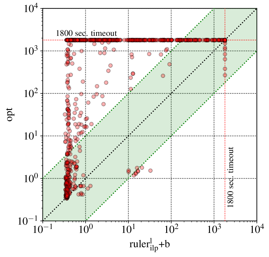
(b) Detailed runtime comparison of $ruler_{{ilp}}^{{l}}$ vs. opt

Figure 1: Scalability of the competitors.

5 Experimental Results

This section evaluates the proposed rule enumeration based approach in terms of scalability and compares it with the state of the art of SAT-based learning of minimum-size decision sets on a variety of publicly available datasets. The experiments were performed in Debian Linux on an Intel Xeon Silver-4110 2.10GHz processor with 64GByte of memory. Following the setup of recent work (Yu et al. 2020), the time limit was set to 1800s for each individual process to run. The memory limit was set to 8GByte per process.

Prototype Implementation and Selected Competition.

A prototype of our rule enumeration based approach was developed as a set of Python scripts, in the following referred to as ruler. The implementation of rule enumeration was done with the use of the state-of-the-art MaxSAT solver RC2 (Ignatiev, Morgado, and Marques-Silva 2018, 2019), which proved to be the most effective in MaxSAT model enumeration (MaxSAT Evaluation 2020). As a result, the terms are computed in a sorted fashion, i.e. the smallest ones come first. For the second phase of the approach, i.e. computing the set cover, we attempted to solve the problem both (1) with the RC2 MaxSAT solver and (2) with the Gurobi ILP solver (Gurobi Optimization 2020). The corresponding configurations of the prototype are called $ruler_{{rc2}}^{{\ast}}$ and $ruler_{{ilp}}^{{\ast}}$, where ‘$\ast$’ can either be ‘r’ or ‘l’ meaning that the solver minimizes either the number of rules or the total number of literals. Configurations $ruler_{{\ast}}^{{\ast}}\text{\it+}b$ apply symmetry breaking constraints to reduce the number of implicant rules computed in the first phase of the approach. Finally, all configurations were set to compute explicit optimal DNF representations for all classes given a dataset.

The competiting approaches include SAT-based methods (Ignatiev et al. 2018) $MinDS_{2}$ and $MinDS_{2}^{\star}$ referred to as $mds_{2}$ and $mds_{2}^{\star}$. The former tool computes the fewest number of rules while the latter lexicographically minimizes the number of rules and then the number of literals. The second competitor is a recent SAT-based approach that minimizes the total number of literals in the model (Yu et al. 2020), in the following referred to as opt. Note that as the main objective of this experimental assessment is to demonstrate scalability of the proposed approach, the methods for computing sparse decision sets (Malioutov and Meel 2018; Ghosh and Meel 2019; Yu et al. 2020) are intentionally excluded due to the significant difference in the problem they tackle.

Benchmarks.

All datasets considered in the evaluation were adopted from  (Yu et al. 2020) and used unchanged. These datasets originated from the UCI Machine Learning Repository (UCI ) and the Penn Machine Learning Benchmarks (PennML ). The total number of datasets is 1065. The number of one-hot encoded (Pedregosa et al. 2011) features (training instances, resp.) per dataset in the benchmark suite varies from 3 to 384 (from 14 to 67557, resp.). Also, since ruler can handle only perfectly classifiable data, it processes each training dataset by keeping the largest consistent (non-overlapping) set of examples. This technique is applied in (Ignatiev et al. 2018; Yu et al. 2020) as well, which enables one to achieve the highest possible accuracy on the training data. Motivated by one of the conclusions of (Yu et al. 2020) stating that perfectly accurate decision sets, if successfully computed, are significantly more accurate than sparse and also heuristic models, here we do not compare test accuracy of the competitors – we assume test accuracy to be (close to) identical for all the considered approaches.

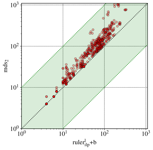
(a) Literals or rules: $ruler_{{ilp}}^{{l}}$ vs. $mds_{2}$

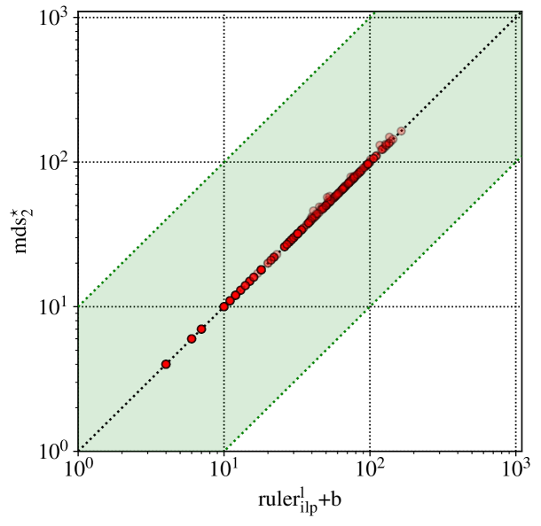
(b) Literals or lexicographic: $ruler_{{ilp}}^{{l}}$ vs. $mds_{2}^{\star}$

Figure 2: Model size comparison.

Raw Performance.

Figure 1(a) shows scalability of all the selected approaches. Observe that the mixed solution $ruler_{{ilp}}^{{r}}\text{\it+}b$ demonstrates the best performance being able to train decision sets for 802 datasets. Second best approach is $ruler_{{ilp}}^{{l}}\text{\it+}b$ and copes with 800 benchmarks. Pure MaxSAT-based $ruler_{{rc2}}^{{r}}\text{\it+}b$ and $ruler_{{rc2}}^{{l}}\text{\it+}b$ perform worse with 734 and 669 instances solved. This is not surprising because the structure of set cover problems naturally fits the capabilities of modern ILP solvers.

Disabling symmetry breaking constraints affects the performance of all configurations of $ruler_{{\ast}}^{{\ast}}$, which drops significantly. When it is disabled, the best such configuration ($ruler_{{ilp}}^{{l}}$) solves 686 benchmarks while the worst one ($ruler_{{rc2}}^{{l}}$) tackles 556. Here, we should say that the maximum and average number of rules enumerated if symmetry breaking is disabled is 326399 and 19604.4, respectively. Breaking symmetric rules decreases these numbers to 8865 and 563.7, respectively.

As for the rivals of the proposed approach, the best of them ($mds_{2}$) is far behind $ruler_{{ilp}}^{{\ast}}\text{\it+}b$ and successfully trains 578 models even though it targets rule minimization, which is arguably a much simpler problem. Another competitor ($mds_{2}^{\star}$) lexicographically minimizes the number of rules and then the number of literals, which is unsurprisingly harder to deal with, as it solves 398 benchmarks. Finally, the worst performance is demonstrated by opt, which learns 351 models. We reemphasize that both opt and $ruler_{{ilp}}^{{l}}\text{\it+}b$ compute minimum-size decision sets in terms of the number of literals. However, the proposed solution outperforms the competition by 449 benchmarks. Note that due to the large encoding size, opt ($mds_{2}$, resp.) is practically limited to optimal models having a few dozens of literals (rules, resp.). There is no such limitation in $ruler_{{\ast}}^{{\ast}}$ – in our experiments, it could obtain minimum-size models having thousands of literals in total within the given time limit. The runtime comparison for $ruler_{{ilp}}^{{l}}\text{\it+}b$ and opt is detailed in Figure 1(b) – observe that except for a few outliers, $ruler_{{ilp}}^{{l}}\text{\it+}b$ outperforms the rival by up to four orders of magnitude.

Rules vs. Literals.

Here we demonstrate that literal minimization results in smaller and thus more interpretable models than rule minimization. Figure 2(a) compares the total number of literals in the models of $mds_{2}$ and $ruler_{{ilp}}^{{l}}\text{\it+}b$ while Figure 2(b) compares the model sizes for $mds_{2}^{\star}$ and $ruler_{{ilp}}^{{l}}\text{\it+}b$. To make a valid comparison, we used only instances solved by both approaches in each pair. Among the datasets used in of Figure 2(a), the average number of literals obtained by $mds_{2}$ and $ruler_{{ilp}}^{{l}}\text{\it+}b$ is 116.2 and 62.2, respectively – the advantage of literal minimization is clear. Also, as shown in Figure 2(b), lexicographic optimization results in models almost identical in size to the models produced by $ruler_{{ilp}}^{{l}}\text{\it+}b$. This suggests that applying the approach of $mds_{2}^{\star}$ may in general pay off in terms of solution size, by significantly sacrificing scalability compared to $mds_{2}$ and, more importantly, to $ruler_{{ilp}}^{{l}}\text{\it+}b$ (398 vs. 578 vs. 800 instances solved, which represents 37.4%, 54.7%, and 75.1% of all 1065 benchmarks, respectively).

6 Conclusions

This paper has introduced a novel approach to learning minimum-size decision sets based on individual rule enumeration. The proposed approach has been motivated by the standard twofold methods applied in two-level logic minimization (Quine 1952, 1955; McCluskey 1956) and split the problem into two parts: (1) exhaustively enumerating individual rules followed by (2) solving the set cover problem. The basic approach has been additionally augmented with symmetry breaking, enabling us to significantly reduce the number of rules produced. The approach has been applied to computing minimum-size decision sets both in terms of the number of rules and in terms of the total number of literals. The proposed approach has been shown to outperform the state of the art in logic-based learning of minimum-size decision sets by a few orders of magnitude.

As the proposed approach targets computing perfectly accurate decision sets, a natural line of future work is to examine ways of applying it to computing sparse decision sets that trade off accuracy for size. Another line of work is to address the issue of potential rule overlap wrt. the proposed approach. Finally, it is of interest to apply similar rule enumeration techniques for devising other kinds of rule-based ML models, e.g. decision lists and decision trees.

References

- ACM (2018) ACM. 2018. Fathers of the Deep Learning Revolution Receive ACM A.M. Turing Award. http://tiny.cc/9plzpz.
- Aglin, Nijssen, and Schaus (2020) Aglin, G.; Nijssen, S.; and Schaus, P. 2020. Learning Optimal Decision Trees Using Caching Branch-and-Bound Search. In AAAI, 3146–3153.
- Angelino et al. (2017) Angelino, E.; Larus-Stone, N.; Alabi, D.; Seltzer, M.; and Rudin, C. 2017. Learning Certifiably Optimal Rule Lists. In KDD, 35–44.
- Bessiere, Hebrard, and O’Sullivan (2009) Bessiere, C.; Hebrard, E.; and O’Sullivan, B. 2009. Minimising Decision Tree Size as Combinatorial Optimisation. In CP, 173–187.
- Biere et al. (2009) Biere, A.; Heule, M.; van Maaren, H.; and Walsh, T., eds. 2009. Handbook of Satisfiability. IOS Press. ISBN 978-1-58603-929-5.
- Brayton et al. (1984) Brayton, R. K.; Hachtel, G. D.; McMullen, C.; and Sangiovanni-Vincentelli, A. 1984. Logic minimization algorithms for VLSI synthesis, volume 2. Springer Science & Business Media.
- Breiman et al. (1984) Breiman, L.; Friedman, J. H.; Olshen, R. A.; and Stone, C. J. 1984. Classification and Regression Trees. Wadsworth. ISBN 0-534-98053-8.
- Bryant et al. (1987) Bryant, R. E.; Beatty, D. L.; Brace, K. S.; Cho, K.; and Sheffler, T. J. 1987. COSMOS: A Compiled Simulator for MOS Circuits. In DAC, 9–16.
- Clark and Boswell (1991) Clark, P.; and Boswell, R. 1991. Rule Induction with CN2: Some Recent Improvements. In EWSL, 151–163.
- Clark and Niblett (1989) Clark, P.; and Niblett, T. 1989. The CN2 Induction Algorithm. Machine Learning 3: 261–283.
- Dash, Günlük, and Wei (2018) Dash, S.; Günlük, O.; and Wei, D. 2018. Boolean Decision Rules via Column Generation. In NeurIPS, 4660–4670.
- Domingos (2015) Domingos, P. 2015. The Master Algorithm: How the Quest for the Ultimate Learning Machine Will Remake Our World. Basic Books. ISBN 978-0465065707.
- (13) Espresso. 1993. Espresso — Multi-valued PLA minimization. http://tiny.cc/txdnsz.
- Fürnkranz, Gamberger, and Lavrac (2012) Fürnkranz, J.; Gamberger, D.; and Lavrac, N. 2012. Foundations of Rule Learning. Springer. ISBN 978-3-540-75196-0.
- Ghosh and Meel (2019) Ghosh, B.; and Meel, K. S. 2019. IMLI: An Incremental Framework for MaxSAT-Based Learning of Interpretable Classification Rules. In AIES, 203–210.
- Gurobi Optimization (2020) Gurobi Optimization, L. 2020. Gurobi Optimizer Reference Manual. URL http://www.gurobi.com.
- Han, Kamber, and Pei (2012) Han, J.; Kamber, M.; and Pei, J. 2012. Data Mining: Concepts and Techniques, 3rd edition. Morgan Kaufmann. ISBN 978-0123814791.
- Hu, Rudin, and Seltzer (2019) Hu, X.; Rudin, C.; and Seltzer, M. 2019. Optimal Sparse Decision Trees. In NeurIPS, 7265–7273.
- Hyafil and Rivest (1976) Hyafil, L.; and Rivest, R. L. 1976. Constructing Optimal Binary Decision Trees is NP-Complete. Inf. Process. Lett. 5(1): 15–17.
- Ignatiev, Morgado, and Marques-Silva (2018) Ignatiev, A.; Morgado, A.; and Marques-Silva, J. 2018. PySAT: A Python Toolkit for Prototyping with SAT Oracles. In SAT, 428–437.
- Ignatiev, Morgado, and Marques-Silva (2019) Ignatiev, A.; Morgado, A.; and Marques-Silva, J. 2019. RC2: an Efficient MaxSAT Solver. J. Satisf. Boolean Model. Comput. 11(1): 53–64.
- Ignatiev et al. (2018) Ignatiev, A.; Pereira, F.; Narodytska, N.; and Marques-Silva, J. 2018. A SAT-Based Approach to Learn Explainable Decision Sets. In IJCAR, 627–645.
- Jabbour et al. (2014) Jabbour, S.; Marques-Silva, J.; Sais, L.; and Salhi, Y. 2014. Enumerating Prime Implicants of Propositional Formulae in Conjunctive Normal Form. In JELIA, 152–165.
- Jordan and Mitchell (2015) Jordan, M. I.; and Mitchell, T. M. 2015. Machine learning: Trends, perspectives, and prospects. Science 349(6245): 255–260.
- Kamath et al. (1992) Kamath, A. P.; Karmarkar, N.; Ramakrishnan, K. G.; and Resende, M. G. C. 1992. A continuous approach to inductive inference. Math. Program. 57: 215–238.
- Karp (1972) Karp, R. M. 1972. Reducibility Among Combinatorial Problems. In Complexity of Computer Computations, 85–103.
- Katz et al. (2017) Katz, G.; Barrett, C. W.; Dill, D. L.; Julian, K.; and Kochenderfer, M. J. 2017. Reluplex: An Efficient SMT Solver for Verifying Deep Neural Networks. In CAV, 97–117.
- Lakkaraju, Bach, and Leskovec (2016) Lakkaraju, H.; Bach, S. H.; and Leskovec, J. 2016. Interpretable Decision Sets: A Joint Framework for Description and Prediction. In KDD, 1675–1684.
- LeCun, Bengio, and Hinton (2015) LeCun, Y.; Bengio, Y.; and Hinton, G. 2015. Deep learning. nature 521(7553): 436.
- Lundberg and Lee (2017) Lundberg, S. M.; and Lee, S. 2017. A Unified Approach to Interpreting Model Predictions. In NIPS, 4765–4774.
- Malioutov and Meel (2018) Malioutov, D.; and Meel, K. S. 2018. MLIC: A MaxSAT-Based Framework for Learning Interpretable Classification Rules. In CP, 312–327.
- Manquinho et al. (1997) Manquinho, V.; Flores, P.; Marques-Silva, J.; and Oliveira, A. 1997. Prime Implicant Computation Using Satisfiability Algorithms. In ICTAI, 232–239.
- MaxSAT Evaluation (2020) MaxSAT Evaluation 2020. 2020. MaxSAT Evaluation 2020. https://maxsat-evaluations.github.io/2020/.
- McCluskey (1956) McCluskey, E. J. 1956. Minimization of Boolean Functions. Bell system technical Journal 35(6): 1417–1444.
- Michalski (1969) Michalski, R. S. 1969. On the quasi-minimal solution of the general covering problem. In International Symposium on Information Processing, 125–128.
- Mitchell (1997) Mitchell, T. M. 1997. Machine learning. McGraw-Hill.
- Mnih et al. (2015) Mnih, V.; Kavukcuoglu, K.; Silver, D.; Rusu, A. A.; Veness, J.; Bellemare, M. G.; Graves, A.; Riedmiller, M.; Fidjeland, A. K.; Ostrovski, G.; et al. 2015. Human-level control through deep reinforcement learning. Nature 518(7540): 529.
- Monroe (2018) Monroe, D. 2018. AI, Explain Yourself. Commun. ACM 61(11): 11–13.
- Narodytska et al. (2018) Narodytska, N.; Ignatiev, A.; Pereira, F.; and Marques-Silva, J. 2018. Learning Optimal Decision Trees with SAT. In IJCAI, 1362–1368.
- Pedregosa et al. (2011) Pedregosa, F.; Varoquaux, G.; Gramfort, A.; Michel, V.; Thirion, B.; Grisel, O.; Blondel, M.; Prettenhofer, P.; Weiss, R.; Dubourg, V.; Vanderplas, J.; Passos, A.; Cournapeau, D.; Brucher, M.; Perrot, M.; and Duchesnay, E. 2011. Scikit-learn: Machine Learning in Python. Journal of Machine Learning Research 12: 2825–2830.
- (41) PennML. 2020. Penn Machine Learning Benchmarks. https://github.com/EpistasisLab/penn-ml-benchmarks.
- Quine (1952) Quine, W. V. 1952. The problem of simplifying truth functions. American mathematical monthly 521–531.
- Quine (1955) Quine, W. V. 1955. A way to simplify truth functions. American mathematical monthly 627–631.
- Quinlan (1986) Quinlan, J. R. 1986. Induction of Decision Trees. Machine Learning 1(1): 81–106.
- Quinlan (1993) Quinlan, J. R. 1993. C4.5: Programs for machine learning. Morgan Kauffmann.
- Ribeiro, Singh, and Guestrin (2016) Ribeiro, M. T.; Singh, S.; and Guestrin, C. 2016. “Why Should I Trust You?”: Explaining the Predictions of Any Classifier. In KDD, 1135–1144.
- Rivest (1987) Rivest, R. L. 1987. Learning Decision Lists. Machine Learning 2(3): 229–246.
- Ruan, Huang, and Kwiatkowska (2018) Ruan, W.; Huang, X.; and Kwiatkowska, M. 2018. Reachability Analysis of Deep Neural Networks with Provable Guarantees. In IJCAI, 2651–2659.
- Rudin and Ertekin (2018) Rudin, C.; and Ertekin, S. 2018. Learning customized and optimized lists of rules with mathematical programming. Mathematical Programming Computation 10: 659–702.
- Shwayder (1975) Shwayder, K. 1975. Combining Decision Rules in a Decision Table. Commun. ACM 18(8): 476–480.
- (51) UCI. 2020. UCI Machine Learning Repository. https://archive.ics.uci.edu/ml.
- Yu et al. (2020) Yu, J.; Ignatiev, A.; Stuckey, P. J.; and Le Bodic, P. 2020. Computing Optimal Decision Sets with SAT. In CP, 952–970.