Ambient Backscatter-Assisted Wireless-Powered Relaying

Abstract

Internet-of-Things (IoT) is featured with low-power communications among a massive number of ubiquitously-deployed and energy-constrained electronics, e.g., sensors and actuators. To cope with the demand, wireless-powered cooperative relaying emerges as a promising communication paradigm to extend data transmission coverage and solve energy scarcity for the IoT devices. In this paper, we propose a novel hybrid relaying strategy by combining wireless-powered communication and ambient backscattering functions to improve applicability and performance of data transfer. In particular, the hybrid relay can harvest energy from radio frequency (RF) signals and use the energy for active transmission. Alternatively, the hybrid relay can choose to perform ambient backscattering of incident RF signals for passive transmission. To efficiently utilize the ambient RF resource, we design mode selection protocols to coordinate between the active and passive relaying in circumstances with and without instantaneous channel gain. With different mode selection protocols, we characterize the success probability and ergodic capacity of a dual-hop relaying system with the hybrid relay in the field of randomly located ambient transmitters. The analytical and the numerical results demonstrate the effectiveness of the mode selection protocols in adapting the hybrid relaying into the network environment and reveal the impacts of system parameters on the performance gain of the hybrid relaying. As applications of our analytical framework which is computationally tractable, we formulate optimization problems based on the derived expressions to optimize the system parameters with different objectives. The optimal solutions exhibit a tradeoff between the maximum energy efficiency and target success probability.

Index terms- Large-scale IoT, wireless-powered relaying, ambient backscatter communications, performance analysis, energy efficiency.

I Introduction

Wireless-powered communication [2, 3, 4, 5, 6] is a green networking paradigm that allows wireless devices to harvest energy from ambient signals, especially radio-frequency (RF) waves. The harvested energy is then used for data transmission without requiring an external energy supply. Therefore, it is considered to be an enabling technology to support machine-type communications (MTC) for Internet-of-Things (IoT) applications [7, 8, 9], such as smart sensors and wearable devices [10]. It has also been shown that for traditional wireless networking, cooperative relaying can improve the reliability of wireless data transmission [11]. This concept is particularly attractive for wireless-powered communication, due to the resource limitation of the devices. In this regard, wireless-powered relaying has attracted a great deal of recent research attention. Existing literature [12, 13, 14, 15] has shown that the use of wireless-powered relaying can provide remarkable performance gains in terms of spatial efficiency and energy efficiency.

However, employing wireless-powered relaying poses some notable challenge. Specifically, a wireless-powered relay involves active transmission, i.e., RF signals are actively generated at the RF front-end. This will require the relay to adopt power-hungry analog circuit components such as oscillator, amplifier, filter, and mixer [16]. Consequently, the relay may need to spend a long time to harvest and accumulate energy for the relaying operation [17]. The situation becomes much worse when the ambient RF signals are weak or intermittent. To solve such issues, some existing literature mainly emphasizes on designing network protocols to utilize network resources more efficiently. For example, the authors in [18] introduced a harvest-then-cooperate protocol for the relay to optimize the time allocation for energy harvesting in a downlink and information forwarding in an uplink to maximize throughput. These network protocols manage to enhance the performance of a wireless-powered relay under different system configurations. However, the performance is still limited by the high circuit power consumption because of the active transmission nature.

To tackle the power consumption limitation caused by active transmission, the work in [19] proposed to integrate the wireless-powered transmission with a passive communication technology, called ambient backscattering. Ambient backscattering, first introduced in [16], can transmit data by passively reflecting the existing RF signals in the air. In particular, ambient backscatter is generated by a load modulator. The load modulator tunes its load impedance to match and mismatch with that of the antenna to absorb and reflect the incident RF signals. Either an absorbing state or reflecting state can be used to indicate a “0” or “1” bit to the backscatter receiver. The incident RF signals can be from existing RF sources such as TV stations, cellular base stations, and Wi-Fi access points. There are three major advantages of ambient backscattering. Firstly, an ambient backscatter transmitter does not actively generate any RF signals and thus require much lower operational power compared with traditional wireless-powered communication based on active transmission. Secondly, an ambient backscatter transmitter utilizes ambient emitters as its carrier sources. Thus, it does not require a dedicated spectrum. Thirdly, an ambient backscatter receiver performs data decoding by averaging the received signals plus modulated backscatter and detect the variations therein for demodulation. Thus, self-interference from the ambient emitters does not significantly degrade the performance of ambient backscatter communication. Therefore, ambient backscattering becomes an effective alternative transmission approach to improve the applicability and energy efficiency of wireless-powered devices [21].

Reference [22] investigated a cognitive radio network where the wireless-powered secondary user is equipped with ambient backscattering capability. In this network, when the primary user is on transmission, the secondary user can either harvest energy or perform ambient backscattering. When the primary user is off, the secondary user can perform active transmission with the harvested energy. Optimal transmission policies are designed to maximize the throughput of the secondary network. Additionally, the work in [46] investigated an integrated wireless-powered transmitter with ambient backscattering for device-to-device communication. It was shown that ambient backscattering is suitable to work as an alternative to wireless-powered transmission when the ambient energy is not sufficient and/or when the interference level is high. However, to the best of our knowledge, none of the existing studies has investigated cooperative relaying enabled with both wireless-powered transmission and ambient backscattering.

This paper investigates a dual-hop cooperative relay system with a hybrid relay that integrates wireless-powered communication and ambient backscattering for data forwarding. Specifically, the hybrid relay first harvests energy from the transmission of ambient emitters, then decodes and forwards the information from the source node to the destination node through either wireless-powered communication or ambient backscattering. The former and the latter are referred to as the wireless-powered relaying (WPR) mode and ambient backscatter relaying (ABR) mode, respectively. As the power for both circuit operation and transmission comes from the ambient RF signals, the performance of the hybrid relay largely depends on the environment factors, e.g., spatial density, distribution, and transmit power of surrounding transmitters and how the relay adapts to them. To analyze and gain insight into operation of the hybrid relaying, we develop analytical models built upon stochastic geometry analysis. In our system model, the ambient emitters and interferers are spatially randomly located following general point processes, i.e., $\alpha$-Ginibre point processes (GPPs) [23]. The processes are able to capture the spatial repulsion among the randomly located points by a repulsion factor $\alpha\in(0,1]$ in which the typical Poisson point process (PPP) cannot do. As aforementioned, the performance of the hybrid relay heavily relies on its ambient environment. Therefore, the repulsion among the ambient transmitters is an important factor that cannot be ignored. In this paper, we adopt $\alpha$-GPP due to its flexibility to evaluate different degrees of repulsion.

Based on the $\alpha$-GPP modeling and analytical framework, our main contributions in this paper are summarized as follows.

• We propose two mode selection protocols that dynamically instruct the hybrid relay to switch between wireless-powered communication and ambient backscattering for the cases with and without instantaneous information of the system. For the former case, the hybrid relay selects the mode based on predefined knowledge and current network conditions. For the latter case, the hybrid relay explores network conditions and uses the learned knowledge to infer future mode selection.

• We derive analytically and computationally tractable expressions to characterize the end-to-end success probability and ergodic capacity of the hybrid relaying system. We demonstrate analytically and numerically that, with the proposed mode selection protocols, wireless-powered communication and ambient backscattering can complement each other to achieve improved performance for cooperative relaying. In particular, for the case with instantaneous channel state information (CSI), the hybrid relaying strictly outperforms both the WPR and the ABR. For the case without instantaneous CSI, the hybrid relaying renders a better performance than the cooperative relaying that randomly selects between the WPR and the ABR.

• We demonstrate an example of our analytical framework in optimal resource allocation of the hybrid relaying system with an objective to maximize the energy efficiency (in bits/Joule), which is the normalized ergodic capacity averaged over the transmit power of the source node. The optimal solutions reveal the tradeoff between the maximum energy efficiency and the achieved success probability.

The remainder of the paper is organized as follows. Section II introduces the system model and the modeling framework. Section III designs mode selection protocols of the hybrid relaying. Section IV and Section V perform the analysis of the hybrid relaying in terms of end-to-end success probabilities and ergodic capacity, respectively, in various settings. Section VI presents the numerical results and demonstrates an applications of our analytical framework in optimizing the system parameters with different objectives. Finally, Section VII concludes our work.

Notations: In this paper, $\mathbb{E}_{X}[\cdot]$ and $\mathbb{E}[\cdot]$ are used to denote the average over the random variable $X$ and all the random variables in $[\cdot]$, respectively. $\mathbb{P}[E]$ denotes the probability that an event $E$ occurs and $\bf{1}$_E is an indicator function that equals 1 if event $E$ occurs and equals 0 otherwise. $\mathbf{x}_{a}$ represents the location of $a$ and $\bar{\mathbf{x}}$ denotes the conjugate of a complex scalar $\mathbf{x}$. $i$ is the imaginary unit, i.e., $i=\sqrt{-1}$. The operator $\|\cdot\|$ represents the Euclidean 2-norm. Besides, let ${n\choose i}=\frac{n(n-1)\cdots(n-i-1)}{i(i-1)\cdots 1}$ denote the binomial coefficient and $[a,b]^{+}\triangleq\max(a,b)$.

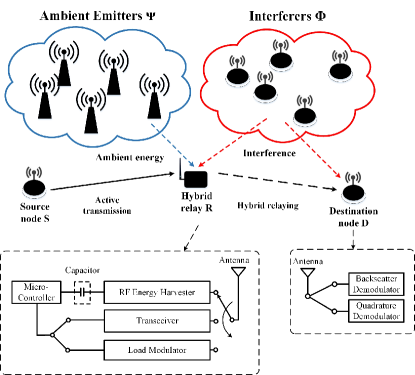
Figure 1: A dual-hop relaying system in an $\alpha$-GPP field of ambient emitters and interferers.

II System Model and Stochastic Geometry Characterization

This section introduces the system model under consideration and then describes some preliminary results of the adopted stochastic geometry framework.

II-A System and Relaying Protocol

As shown in Fig. 1, we consider that a source node $\mathrm{S}$ needs to transmit to a destination node $\mathrm{D}$ which is located far away and cannot achieve a reliable direct communication under its transmit power budget [30]. As such, a hybrid relay $\mathrm{R}$ composed of an active transceiver and an ambient backscatter transmitter is adopted to forward the information from $\mathrm{S}$ to $\mathrm{D}$. Accordingly, $\mathrm{D}$ is equipped with both a quadrature demodulator and backscatter demodulator to decode the information from $\mathrm{R}$. All three nodes $\mathrm{S}$, $\mathrm{R}$, and $\mathrm{D}$ are equipped with a single antenna and work in a half-duplex fashion. Similar to the system models in [31, 32], both $\mathrm{S}$ and $\mathrm{D}$ are assumed to have sufficient energy to supply their operations. Thus, the focus is on $\mathrm{R}$ which is equipped with an energy harvester and an on-board capacitor with capacity $E_{C}$ to store the harvested energy for the relaying operation. We assume the harvested energy can only be consumed in the current time slot and there is no energy left for the subsequent time slot due to capacitor leakage [34, 35].

As shown in the left block diagram in Fig. 1, a time switching-based receiver architecture [33] is adopted to enable $\mathrm{R}$ to work in either energy harvesting, information decoding or transmission. $\mathrm{R}$ performs energy harvesting/ambient backscattering and active transmission on two different frequency bands. For example, the hybrid relay can be designed to harvest energy and perform ambient backscattering by using the downlink signals of ambient base stations (BSs) while the hybrid relay can actively transmit data on the operating frequency of the source node $\mathrm{S}$. Let $\Psi$ and $\Phi$ denote the point processes, i.e., the sets, of ambient emitters and the interferers, respectively. The ambient emitters are the surrounding transmitters working on the frequency band that the hybrid relay performs energy harvesting/ambient backscattering. The interferers are the surrounding transmitters working on the band that the hybrid relay performs active transmission. Let $\widetilde{\zeta}$ ($\zeta$ ) and $\widetilde{P}_{T}$ ($P_{T}$) denote the spatial density and transmit power of the transmitters in $\Psi$ ($\Phi$), respectively. We assume that the distributions of $\Psi$ and $\Phi$ follow independent homogeneous $\alpha$-GPPs [23], which are of a general class of repulsive point process. The mathematical details about $\alpha$-GPP can be found in [23, 36].

Fig. 2 shows the time slots of the relaying protocol adopted by the considered hybrid relaying system to coordinate among energy harvesting and the dual-hop relaying. Let $T$ denote the duration of a time slot. At the beginning of each time slot, an $\omega$ ($0\!<\!\omega\!<\!1$) fraction of $T$ is allocated for $\mathrm{R}$ to harvest ambient energy. Then, the first half and second half of the remaining time (i.e., with duration $\frac{(1-\omega)T}{2}$) are allocated for the source-to-relay transmission and relay-to-destination transmission, respectively. During the relay-to-destination transmission, $\mathrm{R}$ operates in either the WPR mode or the ABR mode, denoted as $\mathrm{W}$ and $\mathrm{A}$, respectively, based on the system environment. The mode selection protocols are to be introduced in Sec. III. If the WPR mode is chosen, $\mathrm{R}$ adopts the decode-and-forward protocol for relaying the data from $\mathrm{S}$ to $\mathrm{D}$ which incurs a circuit power consumption of $E_{\mathrm{W}}\!<\!E_{C}$ per time slot. Otherwise, $\mathrm{R}$ first decodes the active transmission from $\mathrm{S}$ and then forwards the decoded message to $\mathrm{D}$ through ambient backscattering which incurs a circuit power consumption of $E_{\mathrm{A}}\!\ll\!E_{\mathrm{W}}$ per time slot. The hybrid relay is able to function in the WPR mode and ABR mode only if the harvested energy during the energy harvesting phase of each time slot $E_{\mathrm{R}}$ exceeds $E_{\mathrm{W}}$ and $E_{\mathrm{A}}$, respectively.

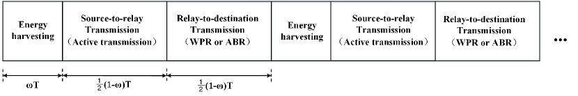
Figure 2: A time-slot based relaying protocol.

II-B Channel Model and SINR/SNR Formulation

All the channels in the systems are considered to experience independent and identically distributed (i.i.d.) block Rayleigh fading. In particular, the fading channel gains follow exponential distributions. Besides, we consider i.i.d. zero-mean additive white Gaussian noise (AWGN) with variance $\widetilde{\sigma}^{2}$ and $\sigma^{2}$ on the transmit frequency of $\Psi$ and $\Phi$, respectively.

II-B1 Harvested Energy

The hybrid relay harvests energy from the ambient emitters in $\Psi$ for its operation. The power of the RF signals from $\Psi$ received by the hybrid relay can be computed as

$$Q_{\mathrm{R}}=\widetilde{P}_{T}\sum_{\mathbf{x}_{k}\in\Psi}\widetilde{h}_{k,\mathrm{R}}\|\mathbf{x}_{k}-\mathbf{x}_{\mathrm{R}}\|^{-\widetilde{\mu}},$$ (1)

where $\widetilde{h}_{a,b}\sim\exp(1)$ is the fading channel gain between nodes $a$ and $b$ on the transmit frequency of $\Psi$, and $\widetilde{\mu}$ represents the path-loss exponent for the signals from the ambient emitters in $\Psi$.

Then, the instantaneous energy harvesting rate (in Watt) at the hybrid relay can be expressed as $\rho_{\mathrm{R}}=\beta Q_{\mathrm{R}}$, where $\beta\in(0,1]$ denotes the RF-to-DC conversion efficiency. And the amount of energy harvested during the energy harvesting phase is obtained as $E_{\mathrm{R}}=\omega T\rho_{\mathrm{R}}$.

II-B2 Source-to-Relay Transmission

During the source-to-relay transmission phase, the receive SINR at the relay node $\mathrm{R}$ is given by

$$\nu_{\mathrm{R}}=\frac{P_{\mathrm{S}}h_{\mathrm{S},\mathrm{R}}d^{-\mu}_{\mathrm{S},\mathrm{R}}}{I_{\mathrm{R}}+\sigma^{2}},$$ (2)

where $P_{\mathrm{S}}$ is the transmit power of the source node, $h_{a,b}\sim\exp(1)$ denotes the fading channel gain between $a$ and $b$ on the transmit frequency of $\Phi$, $d_{x,y}$ represents the distance between $x$ and $y$, $\mu$ is the path-loss exponent for signals from the interferers $\Phi$, $\mathrm{S}$ and $\mathrm{R}$, $I_{\mathrm{R}}=\sum_{j\in\Phi}P_{T}h_{j,\mathrm{R}}\|\mathbf{x}_{j}-\mathbf{x}_{\mathrm{R}}\|^{-\mu}$ is the aggregated interference received at $\mathrm{R}$.

II-B3 Relay-to-Destination Transmission

Let $\rho_{\mathrm{W}}=\frac{E_{\mathrm{W}}}{T}$ and $\rho_{\mathrm{A}}=\frac{E_{\mathrm{A}}}{T}$ denote the average circuit power consumption rate of $\mathrm{R}$ in the WPR mode and the ABR mode, respectively, and $\rho_{C}\triangleq\frac{E_{C}}{T}$ denotes the normalized energy capacity over a time slot duration. Moreover, let us define $\varrho_{\mathrm{W}}\triangleq\frac{\rho_{\mathrm{W}}}{\omega\beta}$, $\varrho_{\mathrm{A}}\triangleq\frac{\rho_{\mathrm{A}}}{\omega\beta}$ and $\varrho_{C}\triangleq\frac{\rho_{C}}{\omega\beta}$. If the WPR mode is chosen, $\mathrm{R}$ uses all the available energy for active transmission during the relay-to-destination transmission phase. Then, the transmit power can be calculated as:

$$P^{\mathrm{W}}_{\mathrm{R}}\!=\!\begin{cases}0&\text{if}\quad\!\!\!Q_{\mathrm{R}}\!\leq\!\varrho_{\mathrm{W}},\\ \frac{T\omega\beta Q_{\mathrm{R}}-E_{\mathrm{W}}}{\frac{T(1-\omega)}{2}}=\frac{2(\omega\beta Q_{\mathrm{R}}-\rho_{\mathrm{W}})}{1-\omega}&\text{if}\quad\!\!\!\varrho_{\mathrm{W}}\!<\!Q_{\mathrm{R}}\!\leq\!\varrho_{\mathrm{W}}+\varrho_{C},\\ \frac{E_{C}}{\frac{T(1-\omega)}{2}}=\frac{2\rho_{C}}{1-\omega}&\text{ otherwise},\end{cases}$$ (3)

Correspondingly, the receive SINR at $\mathrm{D}$ is

$$\nu^{\mathrm{W}}_{\mathrm{D}}=\frac{P^{\mathrm{W}}_{\mathrm{R}}h_{\mathrm{R},\mathrm{D}}d^{-\mu}_{\mathrm{R},\mathrm{D}}}{\sum_{j\in\Phi}P_{T}h_{j,\mathrm{D}}\|\mathbf{x}_{\mathrm{R}}-\mathbf{x}_{\mathrm{D}}\|^{-\mu}\!+\!\sigma^{2}}.$$ (4)

Then, the end-to-end capacity achieved can be computed as

$$C_{\mathrm{W}}\!=\!\begin{cases}\frac{(1-\omega)}{2}W\log_{2}\big{(}1+\nu\big{)}&\text{if}\quad\!\!\!\nu\!\geq\!\tau_{\mathrm{W}},\\ 0&\text{ otherwise},\end{cases}$$ (5)

where $W$ denotes the transmission bandwidth of $\mathrm{R}$ in the WPR mode, $\nu=\min(\nu_{\mathrm{R}},\nu^{\mathrm{W}}_{\mathrm{D}})$, and $\tau_{\mathrm{W}}$ is the minimum SINR threshold to decode data from active transmission at $\mathrm{R}$ and $\mathrm{D}$.

Otherwise, if $\mathrm{R}$ decides to forward data through ambient backscattering, the transmit power of modulated backscatter can be calculated as [37]

$$P^{\mathrm{A}}_{\mathrm{R}}=\eta\xi Q_{\mathrm{R}},$$ (6)

where $\eta$ is the fraction of the incoming RF signals reflected during backscattering and $\xi\in(0,1]$ is the backscattering efficiency of the transmit antenna [38]. $\xi$ represents the portion of the reflected signals that are effectively used to carry the modulated data. The values of $\eta$ and $\xi$ are dependent on the tag-encoding scheme [39] and tag antenna aperture [40], respectively.

The receive signal-to-noise ratio (SNR) from ambient backscatter at $\mathrm{D}$ is

$$\nu^{\mathrm{A}}_{\mathrm{D}}=\frac{P^{\mathrm{A}}_{\mathrm{R}}\widetilde{h}_{\mathrm{R},\mathrm{D}}d^{-\mu}_{\mathrm{R},\mathrm{D}}}{\widetilde{\sigma}^{2}}.$$ (7)

Due to the adopted simple amplitude demodulation based on envelope detection [16], an ambient backscatter receiver typically requires much higher receive SNR to achieve a low bit error rate compared with a quadrature demodulator. For example, a bit error rate around $10^{-3}$ can be obtained with $10$ dB receive SNR [41]. Once the receive SNR at $\mathrm{D}$ is above the threshold $\tau_{\mathrm{A}}$, a pre-designed channel capacity $C_{\mathrm{A}}$ can be attained over the relay-to-destination link. The value of $C_{\mathrm{A}}$ is dependent on the encoding scheme adopted and the setting of the resistor-capacitor of the ambient backscattering circuit [16, 22]. As ambient backscattering usually adopts very simple modulation schemes, such as amplitude shift keying and phase shift keying, it is reasonable to assume that $C_{\mathrm{A}}<C_{\mathrm{W}}$.

Table I summaries the main notations used in this paper.

TABLE I: NOTATIONs.

Symbol	Definition
$\Psi$, $\Phi$	The point processes representing the ambient emitters and interferers, respectively
$\widetilde{\alpha}$, $\alpha$	Repulsion factors for $\Psi$ and $\Phi$, respectively
$\widetilde{P}_{T}$, $P_{T}$	The transmit power of the transmitters in $\Psi$ and $\Phi$, respectively
$P_{\mathrm{S}}$	The transmit power of the source node $\mathrm{S}$
$\widetilde{\sigma}^{2}$, $\sigma^{2}$	The variance of AWGN in the transmit frequency of $\Psi$ and $\Phi$, respectively
$E_{\mathrm{R}}$	The amount of harvested energy at the hybrid relay $\mathrm{R}$
$E_{C}$	The capacitor capacity of $\mathrm{R}$
$\xi$	Backscattering efficiency
$\nu^{\mathrm{W}}_{\mathrm{R}}$, $\nu^{\mathrm{A}}_{\mathrm{R}}$	The receive SINR and SNR at $\mathrm{R}$ from active transmission and ambient backscatter, respectively
$\tau_{\mathrm{W}}$, $\tau_{\mathrm{A}}$	The SINR threshold to decode from active transmission and ambient backscatter, respectively

II-C Preliminaries

This subsection describes some primarily results of $\alpha$-GPP modeling which are applied later in the analysis of this paper. We consider that the hybrid relay $\mathrm{R}$ locates at the origin of the Euclidean space surrounded by the $\alpha$-GPP distributed ambient emitters $\Psi$ with transmit power $\widetilde{P}_{T}$. In the Rayleigh fading environment, the distribution of the received signal power from $\Psi$ at $\mathrm{R}$, i.e., $Q_{\mathrm{R}}$ in (1), are presented in the following proposition.

Proposition 1.

[46, Theorem 1] The probability density function (PDF) and cumulative distribution function (CDF) of $Q_{\mathrm{R}}$ are given, respectively, as:

$$f_{Q_{\mathrm{R}}}(q)=\mathcal{L}^{-1}\Big{\{}\mathrm{Det}\big{(}\mathrm{Id}+\widetilde{\alpha}\mathbb{G}_{\Psi}(\mathbf{x},\mathbf{y})\varpi_{\mathbf{x}}(s)\varpi_{\mathbf{y}}(s)\big{)}^{\!-\frac{1}{\widetilde{\alpha}}}\Big{\}}(q),$$ (8)

and $$F_{Q_{\mathrm{R}}}(q)=\mathcal{L}^{-1}\!\left\{\!\frac{1}{s}\mathrm{Det}\big{(}\mathrm{Id}+\widetilde{\alpha}\mathbb{G}_{\Psi}(\mathbf{x},\mathbf{y})\varpi_{\mathbf{x}}(s)\varpi_{\mathbf{y}}(s)\big{)}^{-\frac{1}{\widetilde{\alpha}}}\!\right\}\!(q),$$ (9)

where $\mathcal{L}^{-1}\{\cdot\}(x)$ represents the inverse Laplace transform which can be evaluated by the Mellin’s inverse formula [42], $\varpi_{\mathbf{z}}(s)\!\triangleq\!\sqrt{\!1\!-\!\big{(}1\!+\!s\widetilde{P}_{T}\|\mathbf{z}\|^{-\widetilde{\mu}}\big{)}^{\!-1}}$, and $\mathbb{G}_{\Psi}(\mathbf{x},\mathbf{y})\triangleq\widetilde{\zeta}\exp\!\left(\!-\frac{\pi\widetilde{\zeta}}{2}(\|\mathbf{x}\|^{2}\!\!+\!\!\|\mathbf{y}\|^{2}\!\!-\!2\mathbf{x}\bar{\mathbf{y}})\!\right)$ is the Ginibre kernel of $\Psi$, which represents the correlation force among different spatial points in $\Psi$.

III Operational Model Selection Protocols

The advantage of the hybrid relay lies in the fact that it can select the more suitable operational mode to achieve better performance under different network conditions. However, as the hybrid relay is a wireless-powered device, any mode selection protocols that have heavy computational complexity, e.g., based on online optimizations [43, 44], are not applicable. For implementation practicality, low complexity mode selection based on obtainable information and limited communication overhead needs to be devised. For the mode selection of the hybrid relay, we consider the situations with and without instantaneous CSI. For the former and the latter situations, we propose two protocols, namely, energy and SINR-aware Protocol (ESAP) and explore-then-commit protocol (ETCP), respectively, for the hybrid relay adapting to the network environment. The operational procedures of the mode selection protocols are specified as follows.

• ESAP: The idea of the ESAP is using ABR to assist data forwarding when the WPR is not feasible (i.e., either when $\mathrm{{R}}$ does not harvest sufficient energy or the forwarded data is not successfully decoded by $\mathrm{D}$) based on the current system conditions. The mode selection of ESAP is done at the end of each energy harvesting phase. In particular, $\mathrm{S}$ first sends preamble signals to $\mathrm{R}$, and $\mathrm{R}$ detects its receive SINR $\nu_{\mathrm{R}}$ and the amount of harvested energy $E_{\mathrm{R}}$ in its capacitor. If $\nu_{\mathrm{R}}>\tau_{\mathrm{R}}$ and $E_{\mathrm{R}}>E_{\mathrm{W}}$, $\mathrm{R}$ transmits preambles to $\mathrm{D}$ through WPR with transmit power $P^{\mathrm{W}}_{\mathrm{R}}=\big{[}\frac{2(E_{\mathrm{R}}-E_{\mathrm{W}})}{(1-\omega)T},\frac{2E_{C}}{(1-\omega)T}\big{]}^{+}$. Otherwise, $\mathrm{R}$ chooses the ABR mode. Upon receiving the preamble signals from $\mathrm{R}$, $\mathrm{D}$ provides a feedback of its receive SINR to $\mathrm{R}$ through signaling. If the receive SINR at $\mathrm{D}$ is greater than $\tau_{\mathrm{W}}$, $\mathrm{R}$ chooses the WPR mode for relaying. Otherwise, $\mathrm{R}$ chooses the ABR mode for relaying. For ESAP, we consider the ideal case that the mode selection at the end of each energy harvesting phase causes negligible time and energy consumption.

• ETCP: The idea of the ETCP is to select the averagely better-performed mode in terms of success probability based on the history information. In particular, ECTP begins with an exploration period that occupies the first initial 2$n$ ($n\in\mathbb{N}+$) to learn the network conditions before committing to a certain operation mode for steady-state transmission based on the learned knowledge. Specifically, in the exploration period, $\mathrm{R}$ works in each operational mode for $n$ time slots in an arbitrary sequence. Afterward, $\mathrm{D}$ feeds back the numbers of successful transmissions in the WPR mode and ABR mode, denoted as $N_{\mathrm{WPR}}$ and $N_{\mathrm{ABR}}$, respectively, to $\mathrm{S}$. Since then, $\mathrm{R}$ always selects the WPR mode, if $N_{\mathrm{WPR}}>N_{\mathrm{ABR}}$, and the ABR mode, if $N_{\mathrm{ABR}}>N_{\mathrm{WPR}}$, and uniformly selects between the ABR and WPR modes at random, otherwise.

Note that both of the proposed mode selection protocols are adopted only at the hybrid relay. ESAP operates based on the information including the physical parameters of $\mathrm{R}$, i.e., $E_{\mathrm{W}}$ and $E_{C}$, and network environment-dependent parameters, i.e., $E_{\mathrm{R}}$, and $\nu_{\mathrm{D}}$. The physical parameters can be known by the relay as predefined knowledge, while the network-dependent parameters can be obtained through detection at the beginning of each time slot. By contrast, ETCP chooses the mode based on the history information without knowing the current channel condition. It can be seen that both mode selection protocols are practical as they are based on information attainable at the hybrid relay.

It is worth mentioning that ESAP incurs much higher overhead than ETCP. In particular, ESAP requires the hybrid relay to know the expression of $P^{\mathrm{W}}_{\mathrm{R}}$ in (3) and values of $\rho_{\mathrm{W}}$ and $\rho_{C}$ and as a priori. Additionally, the hybrid relay with ESAP needs a feedback from the destination node and calculation of $P^{\mathrm{W}}_{\mathrm{R}}$ according to (3) every time slot. By contrast, the hybrid relay with ETCP only needs one feedback from the destination node and one comparison operation between the values of $N_{\mathrm{WPR}}$ and $N_{\mathrm{ABR}}$ after the first 2$n$ initial time slots.

IV Analysis of Success Probability

In this section, we analyze the performance of the hybrid relaying system in presence of randomly located ambient emitters and interferers. For this,

• we first derive the mode selection probabilities of the hybrid relay with the proposed protocols,

• we characterize the interference distribution under the $\alpha$-GPP modeling framework and derive the success probabilities of the hybrid relaying with both ESAP and ETCP,

• and we also simplify the success probabilities in the special cases when one of the operational modes of the hybrid relay is disabled and when the distribution of ambient transmitters follow PPPs.

The transmission of the dual-hop hybrid relaying system is considered to be successful if 1) the relay can harvest sufficient energy for its circuit operation and for decoding information transmitted by the source and 2) the destination can decode the information forwarded by the relay either through active transmission or ambient backscattering. Let $\mathrm{M}\in\{\mathrm{W},\mathrm{A}\}$ denote the operational mode indicator of the hybrid relay $\mathrm{R}$. Mathematically, the success probability of the hybrid relaying is expressed as

$$\mathcal{S}_{\textup{HR}}=\mathbb{P}\Big{[}\nu_{\mathrm{R}}\!>\!\tau_{\mathrm{W}},\nu^{\mathrm{W}}_{\mathrm{D}}\!>\!\tau_{\mathrm{W}},E_{\mathrm{R}}>E_{\mathrm{W}},\mathrm{M}=\mathrm{W}\Big{]}+\mathbb{P}\Big{[}\nu_{\mathrm{R}}\!>\!\tau_{\mathrm{W}},\nu^{\mathrm{A}}_{\mathrm{D}}\!>\!\tau_{\mathrm{A}},E_{\mathrm{R}}>E_{\mathrm{A}},\mathrm{M}\!=\!\mathrm{A}\Big{]}$$

$$\overset{\text{(a)}}{=}\mathbb{P}\Big{[}\nu_{\mathrm{R}}\!>\!\tau_{\mathrm{W}},\nu^{\mathrm{W}}_{\mathrm{D}}\!>\!\tau_{\mathrm{W}},E_{\mathrm{R}}\!>\!E_{\mathrm{W}}|\mathrm{M}\!=\!\mathrm{W}\Big{]}\mathbb{P}\Big{[}\mathrm{M}\!=\!\mathrm{W}\Big{]}\!+\!\mathbb{P}\Big{[}\nu_{\mathrm{R}}\!>\!\tau_{\mathrm{W}},\nu^{\mathrm{A}}_{\mathrm{D}}\!>\!\tau_{\mathrm{A}},E_{\mathrm{R}}\!>\!E_{\mathrm{A}}|\mathrm{M}\!=\!\mathrm{A}\Big{]}\mathbb{P}\Big{[}\mathrm{M}\!=\!\mathrm{A}\Big{]},\!\!\!\!\!$$ (10)

where (a) follows the Bayes’ theorem [45, page 36].

IV-A General-Case Result for ESAP

We first investigate the hybrid relaying with ESAP. Note that with block Rayleigh fading channels, the source-to-relay transmission and relay-to-destination transmission are affected by the same set of interferers with static locations. In other words, the relay and destination nodes experience spatially and temporally correlated interference. In this scenario, we characterize the success probability of hybrid relaying defined in (IV) in the following theorem.

Theorem 1.

The success probability of the hybrid relaying with ESAP is

$$\mathcal{S}^{\textup{ESAP}}_{\textup{HR}}\!=\!\exp\!\Big{(}\!-\!\kappa(\tau_{\mathrm{W}})\sigma^{2}\!\Big{)}\!\Bigg{(}\!\chi_{\mathbb{A}}(\tau_{\mathrm{W}},\rho_{C})\bigg{(}\!1\!-\!F_{Q_{\mathrm{R}}}\big{(}\varrho_{\mathrm{W}}\!+\!\varrho_{C}\big{)}-\!\int^{\infty}_{\!\varrho_{\mathrm{W}}\!+\!\varrho_{C}}\!\delta(q)f_{Q_{\mathrm{R}}}(q)\mathrm{d}q\!\bigg{)}+\!\int^{\varrho_{\mathrm{W}}\!+\!\varrho_{C}}_{\!\varrho_{\mathrm{W}}}\!\!\!\big{(}1\!-\!\delta(q)\big{)}$$

$$\hskip 8.53581pt\!\!\times\chi_{\mathbb{A}}(\tau_{\mathrm{W}},\omega\beta q\!-\!\rho_{\mathrm{W}})f_{Q_{\mathrm{R}}}(q)\mathrm{d}q+\mathrm{Det}\Big{(}\mathrm{Id}\!+\!\alpha\mathbb{G}_{\Phi}(\mathbf{x},\mathbf{y})\psi_{\mathbf{x}}\big{(}\kappa(\tau_{\mathrm{W}})\big{)}\psi_{\mathbf{y}}\big{(}\kappa(\tau_{\mathrm{W}})\big{)}\!\Big{)}^{\!\!-\!\frac{1}{\alpha}}\!\!\!\!\int^{\infty}_{\!\varrho_{\mathrm{A}}}\!\!\!\delta(q)f_{Q_{\mathrm{R}}}(q)\mathrm{d}q\!\Bigg{)},$$ (11)

where $\kappa(v)\!\triangleq\!\frac{d^{\mu}_{\mathrm{S},\mathrm{R}}v}{P_{\mathrm{S}}}$, $\delta(q)\!\triangleq\!\exp\!\Big{(}\!\!-\!\frac{d^{\mu}_{\mathrm{R},\mathrm{D}}\widetilde{\sigma}^{2}\tau_{\mathrm{A}}}{\eta\xi q}\!\Big{)}$, $\mathbb{G}_{\Phi}(\mathbf{x},\mathbf{y})\!\triangleq\!\widetilde{\zeta}\exp\!\Big{(}\!\!-\!\frac{\pi\widetilde{\zeta}}{2}(\|\mathbf{x}\|^{2}\!\!+\!\|\mathbf{y}\|^{2}\!\!-\!2\mathbf{x}\bar{\mathbf{y}})\!\Big{)}$, $\psi_{\mathbf{z}}(s)\!\triangleq\!\sqrt{\!1\!-\!\Big{(}\!1\!+\!sP_{T}\|\mathbf{z}\|^{-\mu}\!\Big{)}^{\!\!-1}}$, $f_{Q_{\mathrm{R}}}(q)$ and $F_{Q_{\mathrm{R}}}(x)$ are given in (8) and (9), respectively, $\chi_{\mathbb{A}}$ is given as:

$$\chi_{\mathbb{A}}(v,p)=\exp\!\Big{(}\!-\ell(v,p)\sigma^{2}\Big{)}\mathrm{Det}\Big{(}\mathrm{Id}\!+\!\alpha\mathbb{G}_{\Phi}(\mathbf{x},\mathbf{y})\varphi_{\mathbf{x}}\big{(}\ell(v,p)\big{)}\varphi_{\mathbf{y}}\big{(}\ell(v,p)\big{)}\!\Big{)}^{\!-\frac{1}{\alpha}},$$ (12)

therein $\ell(v,p)\!\triangleq\!\frac{d^{\mu}_{\mathrm{R},\mathrm{D}}v(1-\omega)}{2p}$, and $\varphi_{\mathbf{z}}(s)\!\triangleq\!\!\sqrt{\!1\!-\!\Big{(}\!1\!+\!\kappa(\tau_{\mathrm{A}})P_{T}\|\mathbf{z}\|^{-\mu}\!\Big{)}^{\!\!\!-1}\!\Big{(}\!1\!+\!sP_{T}\|\mathbf{z}\!-\!\mathbf{x}_{\mathrm{D}}\|^{-\mu}\!\Big{)}^{\!\!\!-1}}$.

For readability, the proof of Theorem 1 is presented in Appendix A.

The analytical expression in (1) appears in terms of the Fredholm determinant [23], which allows an efficient numerical evaluation of the relevant quantities [24, 25, 26]. It is observed that the analytical expression of $\mathcal{S}^{\textup{ESAP}}_{\textup{HR}}$ in (1) has multiple terms. This is due to the fact that the proposed hybrid relaying features with a two-mode operation. The analytical expression involves the joint probabilities that an operational mode is selected and the relay transmission in the selected mode is successful. We note that the analytical expression in (1) has a comparable computational complexity to the analytical results in [46, 47, 48]. The terms that have the highest computational complexity (e.g., the last term in (1)) involve one integral of the inverse Laplace transform of the Fredholm determinant, which can be evaluated relatively easily with numerical integration tools.

IV-B Special-Case Results

Next, we investigate some special settings which considerably simplify the general-case result in (1).

IV-B1 Pure Ambient Backscatter Relaying

In the special case when $\mathrm{R}$ forwards information from $\mathrm{S}$ to $\mathrm{D}$ through ambient backscattering only, referred to as pure ABR, we have the corresponding success probability as follows.

Corollary 1.

The success probability of the pure ABR

$$\mathcal{S}_{\textup{ABR}}\!=\!\exp\!\Big{(}\!\!-\kappa(\tau_{\mathrm{W}})\sigma^{2}\Big{)}\mathrm{Det}\Big{(}\mathrm{Id}\!+\!\alpha\mathbb{G}_{\Phi}(\mathbf{x},\mathbf{y})\psi_{\mathbf{x}}\big{(}\kappa(\tau_{\mathrm{W}})\big{)}\psi_{\mathbf{y}}\big{(}\kappa(\tau_{\mathrm{W}})\big{)}\!\Big{)}^{\!\!-\frac{1}{\alpha}}\!\!\!\int^{\infty}_{\!\varrho_{\mathrm{A}}}\!\delta(q)f_{Q_{\mathrm{R}}}(q)\mathrm{d}q,$$ (13)

where $f_{Q_{\mathrm{R}}}(q)$ is given in (8), respectively.

Proof.

The performance of the pure ABR can be derived by setting $\mathrm{R}$ exclusively in ABR mode for relaying as long as the harvested energy is enough to support the function. Mathematically, by plugging $\mathbb{P}\big{[}\mathrm{M}=\mathrm{W}\big{]}=0$ and $\mathbb{P}\big{[}\mathrm{M}=\mathrm{A}\big{]}=\mathbb{P}\big{[}E_{\mathrm{R}}>E_{\mathrm{A}}]$ into the definition in (IV), the corresponding success probability can be expressed as:

$$\mathcal{S}_{\textup{ABR}}=\mathbb{P}\Big{[}\nu_{\mathrm{R}}\!>\!\tau_{\mathrm{W}},\nu^{\mathrm{A}}_{\mathrm{D}}\!>\!\tau_{\mathrm{A}},E_{\mathrm{R}}\!>\!E_{\mathrm{A}}\Big{]},$$ (14)

which is equivalent to the second term of $\mathcal{S}^{\textup{ESAP}}_{\mathrm{A}}$ in (35) with $E_{\mathrm{W}}$ replaced by $\infty$. Therefore, the analytical expression of $\mathcal{S}_{\textup{ABR}}$ in (13) yields from the derivation of $\mathcal{S}^{\textup{ESAP}}_{\mathrm{A}}$ with the mentioned replacement. ∎

We note that the success probability of the hybrid relaying in (1) can be expanded as follows:

$$\mathcal{S}^{\textup{ESAP}}_{\textup{HR}} =\mathbb{P}\Big{[}\nu_{\mathrm{R}}\!>\!\tau_{\mathrm{W}},\nu^{\mathrm{W}}_{\mathrm{D}}\!>\!\tau_{\mathrm{W}},\nu^{\mathrm{A}}_{\mathrm{D}}\!>\!\tau_{\mathrm{A}},E_{\mathrm{R}}\!>\!E_{\mathrm{W}}\Big{]}+\mathbb{P}\Big{[}\nu_{\mathrm{R}}\!>\!\tau_{\mathrm{W}},\nu^{\mathrm{W}}_{\mathrm{D}}\!>\!\tau_{\mathrm{W}},\nu^{\mathrm{A}}_{\mathrm{D}}\!\leq\!\tau_{\mathrm{A}},E_{\mathrm{R}}\!>\!E_{\mathrm{W}}\Big{]}$$

$$\hskip 28.45274pt+\mathbb{P}\Big{[}\nu_{\mathrm{R}}\!>\!\tau_{\mathrm{W}},\nu^{\mathrm{A}}_{\mathrm{D}}\!>\!\tau_{\mathrm{A}},\nu^{\mathrm{W}}_{\mathrm{D}}\!\leq\!\tau_{\mathrm{W}},E_{\mathrm{R}}\!>\!E_{\mathrm{W}}\Big{]}+\mathbb{P}\Big{[}\nu_{\mathrm{R}}\!>\!\tau_{\mathrm{W}},\nu^{\mathrm{A}}_{\mathrm{D}}\!>\!\tau_{\mathrm{A}},E_{\mathrm{W}}\!\geq\!E_{\mathrm{R}}\!>\!E_{\mathrm{A}}\Big{]}$$

$$=\mathbb{P}\Big{[}\nu_{\mathrm{R}}\!>\!\tau_{\mathrm{W}},\nu^{\mathrm{A}}_{\mathrm{D}}\!>\!\tau_{\mathrm{A}},E_{\mathrm{R}}\!>\!E_{\mathrm{A}}\Big{]}+\mathbb{P}\Big{[}\nu_{\mathrm{R}}\!>\!\tau_{\mathrm{W}},\nu^{\mathrm{W}}_{\mathrm{D}}\!>\!\tau_{\mathrm{W}},\nu^{\mathrm{A}}_{\mathrm{D}}\!\leq\!\tau_{\mathrm{A}},E_{\mathrm{R}}\!>\!E_{\mathrm{W}}\Big{]},$$ (15)

where the first equality follows by expanding the first term of (35) into two cases when $\nu^{\mathrm{A}}_{\mathrm{D}}>\tau_{\mathrm{A}}$ and $\nu^{\mathrm{A}}_{\mathrm{D}}\leq\tau_{\mathrm{A}}$ and the last equality follows by combining the first, the third and the fourth terms before the equality. One finds that the probability representation of $\mathcal{S}_{\textup{ABR}}$ in (14) is exactly the first term of (15). Given that the second term of (15) is always positive, we have the following observation.

Remark 1: The success probability of the hybrid relaying with ESAP is strictly higher than that of the pure ABR.

Let $\mathcal{G}^{\textup{ESAP}}_{\textup{ABR}}$ denote the performance improvement of the hybrid relaying with ESAP over the pure ABR in terms of the success probability, i.e., $\mathcal{G}^{\textup{ESAP}}_{\textup{ABR}}=\mathcal{S}^{\textup{ESAP}}_{\textup{HR}}-\mathcal{S}_{\textup{ABR}}$. In particular, we have

$$\mathcal{G}^{\textup{ESAP}}_{\textup{ABR}}=\exp\!\Big{(}\!-\!\kappa(\tau_{\mathrm{W}})\sigma^{2}\!\Big{)}\!\Bigg{(}\!\underbrace{\chi_{\mathbb{A}}(\tau_{\mathrm{W}},\rho_{C})\bigg{(}\!1\!-\!F_{Q_{\mathrm{R}}}\big{(}\varrho_{\mathrm{W}}\!+\!\varrho_{C}\big{)}-\!\int^{\infty}_{\!\varrho_{\mathrm{W}}\!+\!\varrho_{C}}\!\delta(q)f_{Q_{\mathrm{R}}}(q)\mathrm{d}q\!\bigg{)}}_{\mathcal{G}_{1}}$$

$$\hskip 213.39566pt\!\!+\!\underbrace{\int^{\varrho_{\mathrm{W}}\!+\!\varrho_{C}}_{\!\varrho_{\mathrm{W}}}\!\!\!\big{(}1\!-\!\delta(q)\big{)}\chi_{\mathbb{W}}(\tau_{\mathrm{W}},\omega\beta q\!-\!\rho_{\mathrm{W}})f_{Q_{\mathrm{R}}}(q)\mathrm{d}q}_{\mathcal{G}_{2}}\!\Bigg{)}.$$ (16)

Based on the expansion of the Fredholm determinant in [47, eqn. 14], $\chi_{\mathbb{A}}(\tau_{\mathrm{W}},\rho_{C})$ can be expressed as:

$$\chi_{\mathbb{A}}(\tau_{\mathrm{W}},\rho_{C})\!=\exp\!\bigg{(}\!\!-\!\frac{d^{\mu}_{\mathrm{R},\mathrm{D}}\tau_{\mathrm{W}}(1\!-\!\omega)\sigma^{2}}{2\rho_{C}}\!\bigg{)}\!\prod_{n\geq 0}\!\left(\!1\!+\!\frac{2\alpha(\pi\zeta)^{n+1}}{n!}\!\!\int^{R}_{0}\!\!\frac{\exp(-\pi\zeta r^{2})r^{2n+1}}{\!1\!+\!2\rho_{C}r^{\mu}(d^{\mu}_{\mathrm{R},\mathrm{D}}\tau_{\mathrm{W}}(1\!-\!\omega)P_{T})^{-1}}\mathrm{d}r\!\right)^{\!\!\!-\frac{1}{\alpha}}\!\!\!.$$ (17)

As the repulsion factor $\alpha\in[-1,0)$ and all the other parameters take positive values, it is readily checked that $\chi_{\mathbb{A}}$ is an increasing function of $\varrho_{C}$. Given that the physical capacity of the capacitor, i.e., $\varrho_{\mathrm{W}}+\varrho_{C}$, is fixed, both $\mathcal{G}_{1}$ and $\mathcal{G}_{2}$ in (IV-B1), and thus $\mathcal{G}^{\textup{ESAP}}_{\textup{ABR}}$, increase with $\varrho_{C}$. As a result, $\chi_{\mathbb{A}}$ is a decreasing function of $\varrho_{\mathrm{W}}$. It is also noted that $\varrho_{\mathrm{A}}$ does not appear in the expression of $\mathcal{G}^{\textup{ESAP}}_{\textup{ABR}}$.

Remark 2: According to (IV-B1), the improvement of the hybrid relaying with ESAP over the pure ABR $\mathcal{G}^{\textup{HR}}_{\textup{ABR}}$ can be increased with the reduced circuit power consumption $E_{\mathrm{W}}$, while $\mathcal{G}^{\textup{HR}}_{\textup{ABR}}$ is not affected by any change of the circuit power consumption $E_{\mathrm{A}}$.

Furthermore, considering the special case of Corollary 1 where the distributions of $\Psi$ and $\Phi$ exhibit no repulsion, i.e., the Poisson field of the ambient emitters and interferers with $\widetilde{\alpha}\to 0$ and $\alpha\to 0$, we can simplify $\mathcal{S}_{\textup{ABR}}$ in a closed form.

Corollary 2.

When the path-loss exponent $\mu$ equals $4$, the success probability of the pure ABR in the Poisson field of ambient emitters and interferers is

$$\mathcal{S}_{\textup{ABR}}\!=\!\frac{\pi^{2}}{4}\widetilde{\zeta}\sqrt{\frac{\widetilde{P}_{T}}{N}}\hskip 2.84526pt\exp\!\bigg{(}\!\!-\!\frac{d^{4}_{\mathrm{S},\mathrm{R}}\sigma^{2}\tau_{\mathrm{W}}}{P_{\mathrm{S}}}\!-\frac{\pi^{2}\zeta d^{2}_{\mathrm{S},\mathrm{R}}}{2}\sqrt{\frac{\tau_{\mathrm{W}}P_{T}}{P_{\mathrm{S}}}}\bigg{)}\mathrm{Erf}\Bigg{(}\!\sqrt{\frac{N}{\varrho_{\mathrm{A}}}}\Bigg{)},$$ (18)

where $N\triangleq\frac{d^{4}_{\mathrm{R},\mathrm{D}}\widetilde{\sigma}^{2}\tau_{\mathrm{A}}}{\eta\xi}+\frac{\pi^{4}\zeta^{2}_{Q}\widetilde{P}_{T}}{16}$ and $\mathrm{Erf}(t)=\frac{1}{\sqrt{t}}\int^{t}_{-t}\exp(-x^{2})\mathrm{d}x$ is the error function [49].

The proof of Corollary 2 is presented in $\mathbf{Appendix}$ $\mathbf{B}$.

The closed-form expression in (18) directly reveals the effects of the parameters on the success probability. As the circuit power consumption of the pure ABR is ultra-low, we have $\varrho_{\mathrm{A}}\to 0$, and thus $\mathrm{Erf}\Big{(}\!\sqrt{\frac{N}{\varrho_{\mathrm{A}}}}\Big{)}\to 1$ and $\mathcal{S}_{\textup{ABR}}\!\approx\!\frac{\pi^{2}}{4}\widetilde{\zeta}\sqrt{\frac{\widetilde{P}_{T}}{N}}\hskip 2.84526pt\exp\!\bigg{(}\!\!-\!\frac{d^{4}_{\mathrm{S},\mathrm{R}}\sigma^{2}\tau_{\mathrm{W}}}{P_{\mathrm{S}}}\!-\frac{\pi^{2}\zeta d^{2}_{\mathrm{S},\mathrm{R}}}{2}\sqrt{\frac{\tau_{\mathrm{W}}P_{T}}{P_{\mathrm{S}}}}\bigg{)}$. One easily observes that $\mathcal{S}_{\textup{ABR}}$ is an increasing function of $\widetilde{\zeta}$, $P_{\mathrm{S}}$, and $\widetilde{P}_{T}$, and a decreasing function of $\tau_{\mathrm{W}}$, $\tau_{\mathrm{A}}$, $d_{\mathrm{S},\mathrm{R}}$, $d_{\mathrm{R},\mathrm{D}}$, $\zeta$, and $P_{T}$. Among these parameters, $P_{\mathrm{S}}$ is the only one controllable by the hybrid relaying system. In order to maintain a certain target value for $\mathcal{S}_{\textup{ABR}}$, $P_{\mathrm{S}}$ needs to scale linearly with transmit power $P_{T}$ and at a rate of $P_{\mathrm{S}}\propto\zeta^{2}$ with the spatial density of the interferers.

IV-B2 Pure Wireless-Powered Relaying

Next, we consider another special case when $\mathrm{R}$ forwards information over the relay-to-destination link only with wireless-powered transmission referred to as the pure WPR. The corresponding success probability is given in the following corollary.

Corollary 3.

The success probability of the pure WPR is

$$\mathcal{S}_{\textup{WPR}}\!=\!\exp\!\Big{(}\!\!-\!\kappa(\tau_{\mathrm{W}})\sigma^{2}\!\Big{)}\!\bigg{(}\!\int^{\varrho_{\!\mathrm{W}}+\varrho_{C}}_{\varrho_{\!\mathrm{W}}}\!\!\!\!\chi_{\mathbb{A}}(\tau_{\mathrm{W}},\omega\beta q\!-\!\rho_{\mathrm{W}})f_{Q_{\mathrm{R}}}(q)\mathrm{d}q+\chi_{\mathbb{A}}(\tau_{\mathrm{W}},\rho_{C})\Big{(}\!1\!-\!F_{Q_{\mathrm{R}}}\big{(}\varrho_{\mathrm{W}}\!+\!\varrho_{C}\big{)}\!\Big{)}\!\!\bigg{)},$$ (19)

where $\chi_{\mathbb{A}}$, $F_{Q_{\mathrm{R}}}(x)$, and $f_{Q_{\mathrm{R}}}(p)$ are given in (12), (9), and (8), respectively.

Proof.

The performance of the pure WPR can be obtained by letting $\mathcal{\mathrm{R}}$ forward the information from $\mathrm{S}$ to $\mathrm{D}$ with active transmission only, once the harvested energy is sufficient for the function. Mathematically, we have $\mathbb{P}\big{[}\mathrm{M}=\mathrm{W}\big{]}=\mathbb{P}\Big{[}\nu_{\mathrm{R}}\!>\!\tau_{\mathrm{W}},\nu^{\mathrm{W}}_{\mathrm{D}}\!>\!\tau_{\mathrm{W}},E_{\mathrm{R}}\!>\!E_{\mathrm{W}}\Big{]}$ and $\mathbb{P}\big{[}\mathrm{M}=\mathrm{A}\big{]}=0$. By assigning the above conditions to the definition in (IV), the corresponding success probability can be expressed as:

$$\mathcal{S}_{\textup{WPR}}\!=\!\mathbb{P}\Big{[}\nu_{\mathrm{R}}\!>\!\tau_{\mathrm{W}},\nu^{\mathrm{W}}_{\mathrm{D}}\!>\!\tau_{\mathrm{W}},E_{\mathrm{R}}\!>\!E_{\mathrm{W}}\Big{]},$$ (20)

which is exactly the probability representation of $\mathcal{S}^{\textup{ESAP}}_{\mathrm{W}}$ in (35). Therefore, the analytical expression of $\mathcal{S}_{\textup{WPR}}$ in (19) can be directly obtained from (36). ∎

Remark 3: As the probability representation of $\mathcal{S}_{\textup{WPR}}$ in (20) is exactly $\mathcal{S}^{\textup{ESAP}}_{\mathrm{W}}$ in (35), we have $\mathcal{S}^{\textup{ESAP}}_{\textup{HR}}=\mathcal{S}^{\textup{ESAP}}_{\mathrm{W}}+\mathcal{S}^{\textup{ESAP}}_{\mathrm{A}}>\mathcal{S}_{\textup{WPR}}$, given that $\mathcal{S}^{\textup{ESAP}}_{\mathrm{A}}$ is positive. Therefore, the success probability of the hybrid relaying with ESAP is strictly higher than that of the pure WPR.

Let $\mathcal{G}^{\textup{HR}}_{\textup{WPR}}$ denote the performance improvement of the hybrid relaying over the pure WPR in terms of the success probability, i.e., $\mathcal{G}^{\textup{ESAP}}_{\textup{WPR}}=\mathcal{S}^{\textup{ESAP}}_{\textup{HR}}-\mathcal{S}_{\textup{WPR}}$. In particular, we have

$$\mathcal{G}^{\textup{ESAP}}_{\textup{WPR}}=\exp\!\Big{(}\!-\!\kappa(\tau_{\mathrm{W}})\sigma^{2}\!\Big{)}\!\Bigg{(}\!\underbrace{\mathrm{Det}\Big{(}\mathrm{Id}\!+\!\alpha\mathbb{G}_{\Phi}(\mathbf{x},\mathbf{y})\psi_{\mathbf{x}}\big{(}\kappa(\tau_{\mathrm{W}})\big{)}\psi_{\mathbf{y}}\big{(}\kappa(\tau_{\mathrm{W}})\big{)}\!\Big{)}^{\!\!-\!\frac{1}{\alpha}}}_{\mathcal{G}_{3}}\!\int^{\infty}_{\!\varrho_{\mathrm{A}}}\!\!\delta(q)f_{Q_{\mathrm{R}}}(q)\mathrm{d}q$$

$$\hskip 71.13188pt\!-\underbrace{\chi_{\mathbb{A}}(\tau_{\mathrm{W}},\rho_{C})\bigg{(}\!\int^{\infty}_{\!\varrho_{\mathrm{W}}\!+\!\varrho_{C}}\!\delta(q)f_{Q_{\mathrm{R}}}(q)\mathrm{d}q+\!\int^{\varrho_{\mathrm{W}}\!+\!\varrho_{C}}_{\!\varrho_{\mathrm{W}}}\!\delta(q)\chi_{\mathbb{A}}(\tau_{\mathrm{W}},\omega\beta q\!-\!\rho_{\mathrm{W}})f_{Q_{\mathrm{R}}}(q)\mathrm{d}q\bigg{)}}_{\mathcal{G}_{4}}\!\Bigg{)}.$$ (21)

Recall that $\chi_{\mathbb{A}}$ is a decreasing function of $\varrho_{\mathrm{W}}$ from Remark 2. Given that the overall capacity of the capacitor is fixed, i.e., $\varrho_{\mathrm{W}}+\varrho_{C}$, it is readily checked that $\mathcal{G}_{4}$ decreases with $\varrho_{\mathrm{W}}$. Hence, $\mathcal{G}^{\textup{ESAP}}_{\textup{WPR}}$ is an increasing function of $\varrho_{\mathrm{W}}$. In addition, we have $\frac{\partial{\mathcal{G}^{\textup{ESAP}}_{\textup{WPR}}}}{\partial{\varrho_{\mathrm{A}}}}=-\exp\!\big{(}\!-\!\kappa(\tau_{\mathrm{W}})\sigma^{2}\big{)}\mathcal{G}_{3}\delta(\varrho_{\mathrm{A}})f_{Q_{\mathrm{A}}}(\varrho_{\mathrm{A}})<0$. Thus, $\mathcal{G}^{\textup{ESAP}}_{\textup{WPR}}$ is a decreasing function of $\varrho_{\mathrm{A}}$.

Remark 4: It is observed from (IV-B2) that the improvement of the hybrid relaying with ESAP over the pure WPR becomes more remarkable with increased circuit power consumption $E_{\mathrm{W}}$ and reduced circuit power consumption $E_{\mathrm{A}}$.

IV-C General-Case Results for ETCP

Next, we continue to investigate the performance of hybrid relaying with ETCP at the steady states when $\mathrm{R}$ has committed to a certain mode based on its selection criteria. The mode selection probability of ETCP depends on the average success probabilities of the pure ABR and WPR, which have been obtained in $\mathbf{Corollary}$ 1 and $\mathbf{Corollary}$ 3, respectively. Based on these results with ETCP, we have the success probability of hybrid relaying in the following theorem.

Theorem 2.

The success probability of the hybrid relaying with ETCP at the steady states is

$$\mathcal{S}^{\textup{ETCP}}_{\textup{HR}}\!=\frac{1}{2}(\mathcal{S}_{\textup{WPR}}+\mathcal{S}_{\textup{ABR}})+\frac{1}{2}\Big{(}\phi_{1}\big{(}\mathcal{S}_{\textup{WPR}}\big{)}\phi_{2}\big{(}\mathcal{S}_{\textup{ABR}}\big{)}-\phi_{1}\big{(}\mathcal{S}_{\textup{ABR}}\big{)}\phi_{2}\big{(}\mathcal{S}_{\textup{WPR}}\big{)}\Big{)}(\mathcal{S}_{\textup{WPR}}-\mathcal{S}_{\textup{ABR}}),$$ (22)

where $n\in\mathbb{N}^{+}$, $\mathcal{S}_{\textup{ABR}}$ and $\mathcal{S}_{\textup{WPR}}$ are given in (13) and (19), respectively, and $\phi_{1}$ and $\phi_{2}$ are given, respectively, as

$$\phi_{1}(x)=\sum^{n}_{i=1}{n\choose i}x^{i}(1-x)^{n-i}\quad\text{and}\quad\phi_{2}(x)=\sum^{i}_{j=1}{n\choose i\!-\!j}x^{i-j}(1-x)^{n-i+j}.$$

The proof of Theorem 2 can be found in Appendix C.

When the hybrid relay uniformly selects between the ABR and WPR modes at random, the corresponding success probability can be easily obtained by averaging the success probabilities of the two modes, i.e., $\mathcal{S}^{\textup{URMS}}_{\textup{HR}}=\frac{1}{2}(\mathcal{S}_{\textup{ABR}}+\mathcal{S}_{\textup{WPR}})$. Let $\Upsilon\triangleq\mathcal{S}^{\textup{ETCP}}_{\textup{HR}}-\mathcal{S}^{\textup{URMS}}_{\textup{HR}}=\frac{1}{2}\Big{(}\phi_{1}\big{(}\mathcal{S}_{\mathrm{R}}\big{)}\phi_{2}\big{(}\mathcal{S}_{\textup{WPR}}\big{)}-\phi_{1}\big{(}\mathcal{S}_{\textup{WPR}})\phi_{2}\big{(}\mathcal{S}_{\textup{ABR}}\big{)}\Big{)}(\mathcal{S}_{\textup{WPR}}-\mathcal{S}_{\textup{ABR}})$. It is readily checked that $\phi_{1}\big{(}\mathcal{S}_{\textup{WPR}}\big{)}\phi_{2}\big{(}\mathcal{S}_{\textup{ABR}}\big{)}-\phi_{1}\big{(}\mathcal{S}_{\textup{ABR}})\phi_{2}\big{(}\mathcal{S}_{\textup{WPR}}\big{)}$ and $\mathcal{S}_{\textup{WPR}}-\mathcal{S}_{\textup{ABR}}$ take positive, negative, or zero at the same time. Therefore, we have $\Upsilon\geq 0$, which yields the following observation.

Remark 5: The success probability of the hybrid relaying with ETCP is strictly no worse than that with uniformly random mode selection.

V Analysis of Ergodic Capacity

This section investigates the end-to-end ergodic capacity that can be achieved from the hybrid relaying. Specifically, we provide the general-case results for hybrid relaying with ESAP and ETCP and the special-case results for pure ABR and WPR.

The ergodic capacity of the hybrid relaying can be defined as:

$$\mathcal{C}_{\textup{HR}}\triangleq\frac{(1-\omega)}{2}\Big{(}C_{\mathrm{W}}\mathbb{P}\big{[}\mathrm{M}=\mathrm{W}\big{]}+C_{\mathrm{A}}\mathbb{P}\big{[}\mathrm{M}=\mathrm{A}\big{]}\Big{)}$$

$$\!\!\!=\frac{(1-\omega)}{2}\Big{(}\mathbb{E}\Big{[}W\log_{2}(1+\nu)\big{|}\mathrm{M}=\mathrm{W}\Big{]}\mathbb{P}[\mathrm{M}\!=\!\mathrm{W}]\!+\!C_{\mathrm{A}}\mathbb{P}\Big{[}\nu_{\mathrm{R}}>\tau_{\mathrm{W}},\nu^{\mathrm{A}}_{\mathrm{D}}>\tau_{\mathrm{A}}|\mathrm{M}\!=\!\mathrm{A}\Big{]}\mathbb{P}\big{[}\mathrm{M}\!=\!\mathrm{A}\big{]}\Big{)},\!\!$$ (23)

where the coefficient $\frac{1-\omega}{2}$ comes from the fact that the transmission for each hop occupies $\frac{1-\omega}{2}$ fraction of a time slot duration and the last equality follows the assumption that $C_{\mathrm{A}}\ll C_{\mathrm{W}}$.

V-A General-Case Results for ESAP

According to the definition in (V), the ergodic capacity of the hybrid relaying with ESAP is presented in the following theorem.

Theorem 3.

The ergodic capacity of the hybrid relaying with ESAP is

$$\mathcal{C}_{\textup{HR}}\!=\!\frac{1\!-\!\omega}{2}\Bigg{(}\frac{W}{\ln(2)}\!\int^{\infty}_{\tau_{\mathrm{W}}}\frac{\exp\!\big{(}\!-\kappa(v)\sigma^{2}\big{)}}{1+v}\bigg{(}\!\chi_{\mathbb{A}}(v,\rho_{C})\Big{(}1\!-\!F_{Q_{\mathrm{R}}}\big{(}\varrho_{\mathrm{W}}\!+\!\varrho_{C}\big{)}\!\Big{)}\!+\!\int^{\varrho_{\mathrm{W}}+\varrho_{C}}_{\!\varrho_{\mathrm{W}}}\!\!\!\!\chi_{\mathbb{A}}(v,\omega\beta q\!-\!\rho_{\mathrm{W}})$$

$$\hskip 312.9803pt\times f_{Q_{\mathrm{R}}}(q)\mathrm{d}q\!\bigg{)}\mathrm{d}v+\!C_{\mathrm{A}}\mathcal{S}^{\textup{ESAP}}_{\mathrm{A}}\Bigg{)},$$ (24)

where $\chi_{\mathbb{A}}$, $F_{Q_{\mathrm{R}}}(x)$, $f_{Q_{\mathrm{R}}}(q)$, and $\mathcal{S}^{\textup{ESAP}}_{\mathrm{A}}$ are given in (12), (9), (8), and (37), respectively.

The proof of $\mathbf{Theorem}$ 3 is presented in $\mathbf{Appendix}$ $\mathbf{D}$.

V-B Special-Case results

For the analysis of the ergodic capacity, we also investigate the special cases when $\mathrm{R}$ relays the information from $\mathrm{S}$ to $\mathrm{D}$ by using only ambient backscattering or only wireless-powered transmission. In particular, the result of the former case is presented in the following corollary.

Corollary 4.

The capacity of the pure ABR is

$$\mathcal{C}_{\textup{ABR}}\!=\!\frac{(1\!-\!\omega)C_{\mathrm{A}}}{2}\exp\!\Big{(}\!-\!\kappa(\tau_{\mathrm{W}})\sigma^{2}\!\Big{)}\mathrm{Det}\Big{(}\mathrm{Id}\!+\!\alpha\mathbb{G}_{\Phi}(\mathbf{x},\mathbf{y})\psi_{\mathbf{x}}\big{(}\kappa(\tau_{\mathrm{W}})\big{)}\psi_{\mathbf{y}}\big{(}\kappa(\tau_{\mathrm{W}})\big{)}\!\Big{)}^{\!\!-\!\frac{1}{\alpha}}\!\!\!\int^{\infty}_{\!\varrho_{\mathrm{A}}}\!\!\!\delta(q)f_{Q_{\mathrm{R}}}(q)\mathrm{d}q,\!\!$$ (25)

where $f_{Q_{\mathrm{R}}}(q)$ is given in (8).

Proof.

If the relay-to-destination transmission is performed only through ambient backscattering, we have

$$\mathbb{P}[\mathrm{M}=\mathrm{W}]=0\quad\text{and}\quad\mathbb{P}[\mathrm{M}=\mathrm{A}]=\mathbb{P}\big{[}\nu_{\mathrm{R}}\!>\!\tau_{\mathrm{A}},\nu^{\mathrm{A}}_{\mathrm{D}}\!>\!\tau_{\mathrm{A}},E_{\mathrm{R}}\!>\!E_{\mathrm{A}}\big{]}=\mathcal{S}_{\textup{ABR}},$$ (26)

By assigning (26) into the definition in (V), we have the corresponding ergodic capacity as:

$$\mathcal{C}_{\textup{ABR}}=\frac{1-\omega}{2}C_{\mathrm{A}}\mathcal{S}_{\textup{ABR}},$$ (27)

where $\mathcal{S}_{\textup{ABR}}$ has been obtained in Corollary 1.

Subsequently, $\mathcal{C}_{\textup{ABR}}$ in (25) directly yields by inserting $\mathcal{S}_{\textup{ABR}}$ in (13) into (27). ∎

Moreover, if $\mathrm{R}$ performs relaying with only the wireless-powered transmission, we have the capacity of the pure WPR in the following corollary.

Corollary 5.

The capacity of the pure WPR is

$$\mathcal{C}_{\textup{WPR}}\!=\!\frac{W(1\!-\!\omega)}{2\ln(2)}\!\int^{\infty}_{\tau_{\mathrm{W}}}\!\frac{\exp\!\big{(}\!-\kappa(v)\sigma^{2}\big{)}}{1+v}\!\bigg{(}\!\chi_{\mathbb{A}}(v,\rho_{C})\Big{(}1\!-\!F_{Q_{\mathrm{R}}}\big{(}\varrho_{\mathrm{W}}\!+\!\varrho_{C}\big{)}\!\Big{)}$$

$$\hskip 256.0748pt+\!\!\!\int^{\varrho_{\mathrm{W}}+\varrho_{C}}_{\!\varrho_{\mathrm{C}}}\!\!\!\chi_{\mathbb{A}}(v,\omega\beta q\!-\!\rho_{\mathrm{W}})f_{Q_{\mathrm{R}}}(q)\mathrm{d}q\!\bigg{)}\mathrm{d}v,$$ (28)

where $\chi_{\mathbb{A}}$, $F_{Q_{\mathrm{R}}}(x)$, and $f_{Q_{\mathrm{R}}}(q)$ are given in (12), (9), and (8), respectively.

Proof.

From the proof of Corollary 5, we have the conditions that $\mathrm{R}$ only performs WPR as:

$$\mathbb{P}\big{[}\mathrm{M}=\mathrm{W}\big{]}=\mathbb{P}\Big{[}\nu_{\mathrm{R}}\!>\!\tau_{\mathrm{W}},E_{\mathrm{R}}\!>\!E_{\mathrm{W}},\nu^{\mathrm{W}}_{\mathrm{D}}\!>\!\tau_{\mathrm{W}}\Big{]}\quad\text{and}\quad\mathbb{P}\big{[}\mathrm{M}=\mathrm{A}\big{]}=0.$$ (29)

By inserting (29) into (V), we have

$$\mathcal{C}_{\textup{WPR}}=\frac{(1-\omega)}{2}\mathbb{E}\Big{[}W\log_{2}(1+\nu)\mathbf{1}_{\{\nu_{\mathrm{R}}>\tau_{\mathrm{W}},\nu^{\mathrm{W}}_{\mathrm{D}}>\tau_{\mathrm{W}},E_{\mathrm{R}}>E_{\mathrm{W}}\}}\Big{]},$$ (30)

where $\mathbb{E}\Big{[}W\log_{2}(1+\nu)\mathbf{1}_{\{\nu_{\mathrm{R}}>\tau_{\mathrm{W}},\nu^{\mathrm{W}}_{\mathrm{D}}>\tau_{\mathrm{W}},E_{\mathrm{R}}>E_{\mathrm{W}}\}}\Big{]}$ has been obtained in (45). We, therefore, have $\mathcal{C}_{\textup{WPR}}$ in (5) by plugging (45) into (30). ∎

V-C General-Case Results for ETCP

Theorem 4.

The ergodic capacity of the hybrid relaying with ETCP at the steady states is

$$\mathcal{C}^{\textup{ETCP}}_{\textup{HR}}=\frac{1}{2}(\mathcal{C}_{\textup{ABR}}+\mathcal{C}_{\textup{WPR}})+\frac{1}{2}\Big{(}\phi_{1}(\mathcal{S}_{\textup{WPR}})\phi_{2}(\mathcal{S}_{\textup{ABR}})-\phi_{1}(\mathcal{S}_{\textup{ABR}})\phi_{2}(\mathcal{S}_{\textup{WPR}})\Big{)}(\mathcal{C}_{\textup{WPR}}-\mathcal{C}_{\textup{ABR}}),$$ (31)

where $\mathcal{C}_{\textup{ABR}}$, $\mathcal{C}_{\textup{WPR}}$, $\mathcal{S}_{\textup{ABR}}$, and $\mathcal{S}_{\textup{WPR}}$ have been obtained in (25), (5), (13), and (19), respectively.

Proof.

Recall that, from the proof of Theorem 2, we have obtained the probability of $\mathrm{R}$ selecting the ABR mode and WPR mode under ETCP at the steady states in (VII-C) and (43), respectively. According to the mode selection criteria of ETCP described in Section II, the ergodic capacity of the hybrid relaying with ETCP at the steady states can be expressed as

$$\mathcal{C}^{\textup{ETCP}}_{\textup{HR}}=\frac{1}{2}(\mathcal{C}_{\textup{ABR}}+\mathcal{C}_{\textup{WPR}})+\frac{1}{2}(\mathbb{P}[N_{\textup{WPR}}>N_{\textup{ABR}}]-\mathbb{P}[N_{\textup{ABR}}>N_{\textup{WPR}}])(\mathcal{C}_{\textup{WPR}}-\mathcal{C}_{\textup{ABR}}),$$ (32)

By inserting the expressions of $\mathbb{P}[N_{\textup{ABR}}>N_{\textup{WPR}}]$, $\mathbb{P}[N_{\textup{WPR}}>N_{\textup{ABR}}]$, $\mathcal{C}_{\textup{ABR}}$, and $\mathcal{C}_{\textup{WPR}}$ obtained in (VII-C), (43), (25), and (5), respectively, into (32), we have the expression of $\mathcal{C}^{\textup{ETCP}}_{\textup{HR}}$ in (31). ∎

VI Numerical Results

In this section, we show numerical results to validate and evaluate the success probabilities and ergodic capacity of the hybrid relaying system analyzed in Section IV. To demonstrate the advantage of the proposed hybrid relaying with the mode selection protocols, we compare their performance with that of the pure WPR, and the pure ABR. The performance results of the hybrid relaying with ESAP and those with ETCP, the pure WPR and the pure ABR are labeled as “HR-EASP”, “HR-ETCP”, “WPR” and “ABR”, respectively. In the simulation, the ambient emitters $\Psi$ and interferers $\Phi$ are distributed on a circular disc of radius $R=500$ m with the relay node $\mathrm{R}$ centered at the origin. Besides, the source node $\mathrm{S}$ and destination node $\mathrm{D}$ are placed at (-$d_{\mathrm{S},\mathrm{R}}$,0) and ($d_{\mathrm{R},\mathrm{D}}$,0), respectively. $\Psi$ and $\Phi$ are considered as base stations and sensor devices with transmit power $\widetilde{P}_{T}=40$ dBm and $P_{T}=20$ dBm, respectively. The frequency bandwidth of $\Psi$ and $\Phi$ are set as 20 MHz [52] and 50 kHz [53], respectively. The noise variance is -120 dBm/Hz. We set the transmit power of the source node as $P_{\mathrm{S}}=P_{T}$. If the WPR is adopted, the average circuit power consumption rate of $\mathrm{R}$ is set at $\rho_{\mathrm{W}}=50\mu W$, which is within the typical power consumption range of a wireless-powered transmitter [54]. For the ABR, we set $\rho_{\mathrm{A}}=5\mu W$, an order of magnitude smaller than $\rho_{\mathrm{W}}$. The normalized capacitor capacity $\rho_{C}$ is $0.02$ Joules/second. The other system parameters adopted are listed in Table II unless otherwise stated.

TABLE II: Parameter Setting.

Symbol	$\alpha$	$\widetilde{\alpha}$	$\mu$	$\widetilde{\mu}$	$d_{\mathrm{S},\mathrm{R}}$, $d_{\mathrm{R},\mathrm{D}}$	$\tau_{\mathrm{W}}$	$\tau_{\mathrm{A}}$	$\eta$	$\beta$	$\xi$	$\omega$	$C_{\mathrm{A}}$
Value	-0.5	-1	3.5	3.0	5 m	0 dB	20 dB	0.375	0.5	0.25	0.4	50 kbps

VI-1 SINR Threshold on Success Probability

In Fig. 3, the success probabilities $\mathcal{S}^{\textup{ESAP}}_{\textup{HR}}$ and $\mathcal{S}^{\textup{ETCP}}_{\textup{HR}}$ obtained in $\mathbf{Theorem}$ 1 and $\mathbf{Theorem}$ 2, respectively, are shown as functions of the SINR threshold $\tau_{\mathrm{W}}$. To demonstrate the accuracy of the analytical expressions, we compare them with the results generated by Monte Carlo simulations. It can be seen that for both $\mathcal{S}^{\textup{ESAP}}_{\textup{HR}}$ and $\mathcal{S}^{\textup{ETCP}}_{\textup{HR}}$, the analytical results match closely with the simulation results over a wide range of $\tau_{\mathrm{W}}$ and $\tau_{\mathrm{A}}$. Fig. 3(b) depicts $\mathcal{S}^{\textup{ETCP}}_{\textup{HR}}$ under different settings of $n$. For comparison, we also show the success probability of uniform random mode selection, i.e., $\mathcal{S}^{\textup{URMS}}_{\textup{HR}}=\frac{1}{2}(\mathcal{S}_{\textup{ABR}}+\mathcal{S}_{\textup{WPR}})$, labeled as “URMS”. It can be found that $\mathcal{S}_{\textup{ETCP}}$ under different settings of $n$ outperforms all $\mathcal{S}^{\textup{URMS}}_{\textup{HR}}$, which agrees with $\mathbf{Remark}$ $\mathbf{5}$. Moreover, $\mathcal{S}_{\textup{ETCP}}$ monotonically increases with $n$. This is due to the fact that the more number of the time slots to explore, the higher chance the hybrid relay finds the averagely better-performed mode. We can see that the performance gap resulted from the increase of $n$ decreases when $n$ is large. In the following simulations, the value of $n$ is set as 5 to avoid a lengthy exploration period.

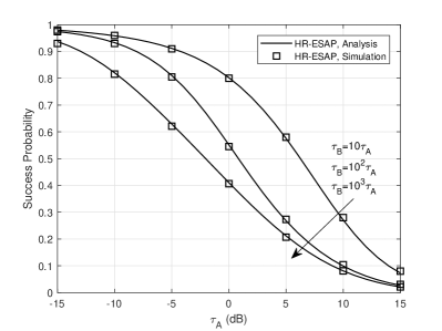
(a) ESAP

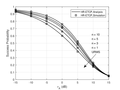
(b) ETCP ($\tau_{\mathrm{A}}=10\tau_{\mathrm{W}}$)

Figure 3: Success probability as a function of $\tau_{\mathrm{W}}$.

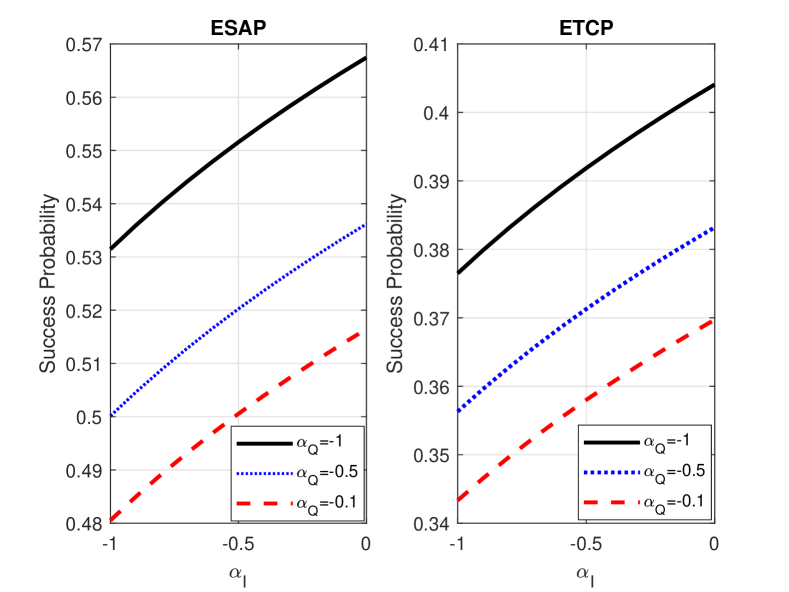
Figure 4: Success probability as a function of $\alpha$.

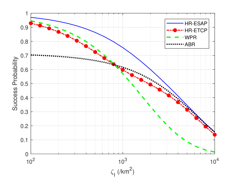
Figure 5: Success probability as a function of $\zeta$. ($\widetilde{\zeta}=2000$/km²)

VI-2 Impact of System Environment (i.e., repulsion factors $\widetilde{\alpha}$ and $\alpha$ and densities $\widetilde{\zeta}$ and $\zeta$ of $\Psi$ and $\Phi$) on Success Probability

Fig. 5 shows the success probabilities $\mathcal{S}^{\textup{ESAP}}_{\textup{HR}}$ and $\mathcal{S}^{\textup{ETCP}}_{\textup{HR}}$ as functions of $\alpha$ under different $\widetilde{\alpha}$. It can be found that greater repulsion among the ambient emitters $\Psi$, i.e., smaller $\widetilde{\alpha}$, increases the success probabilities. By contrast, greater repulsion among the interferers $\Phi$ decreases the success probabilities. This comes from the fact that, given the spatial density, larger repulsion among the transmitters in $\Psi$ ($\Phi$) results in the higher probability that some transmitters in $\Psi$ ($\Phi$) locate near $\mathrm{R}$, and thus stronger received signals from $\Psi$ ($\Phi$). As a result, smaller $\widetilde{\alpha}$ leads to more carrier signals for energy harvesting and smaller $\alpha$ generates more interference at $\mathrm{R}$.

Fig. 5 studies how the success probabilities vary under different density of interferers $\zeta$. As expected, the success probabilities monotonically deceases with $\zeta$. We observe that the hybrid relaying with ESAP achieves a higher success probability than that of the pure ABR and the pure WPR, which corroborates the $\mathbf{Remark}$ $\mathbf{1}$ and $\mathbf{Remark}$ $\mathbf{3}$, respectively. Given the knowledge of receive SINR at the destination node, ESAP can switch the hybrid relay to the ABR mode when the detected interference is high. Therefore, the hybrid relaying with ESAP outperforms the pure WPR and achieves comparable performance with the pure ABR when $\zeta$ is large, e.g., $\zeta=10^{4}$/km², as shown in Fig. 5. For the hybrid relaying with ETCP, $\mathcal{S}^{\textup{ETCP}}_{\textup{HR}}$ approaches the better-performed one than the worse-performed one in most conditions, which demonstrates the effectiveness of the exploration period in determining the better-performed mode. For the pure ABR, it is worth noting that, though the interference on the transmit frequency of $\Phi$ does not affect the ABR link on the transmit frequency of $\Psi$, the interference still affects the source-to-relay link and thus $\mathcal{S}_{\textup{ABR}}$. Since only the source-to-relay link is affected, $\mathcal{S}_{\textup{ABR}}$ is more robust to the impact of increased interference than $\mathcal{S}_{\textup{WPR}}$. This is evident from Fig. 5 that $\mathcal{S}_{\textup{ABR}}$ decreases with the increase of $\rho_{I}$ at a much slower rate than that of $\mathcal{S}_{\textup{WPR}}$.

Fig. 7 examines the impact of the density of the ambient emitters $\widetilde{\zeta}$. In contrast to the influence of $\zeta$, the increase of $\widetilde{\zeta}$ augments the success probabilities of all types of relaying. The reason is that a larger $\widetilde{\zeta}$ increases not only the harvested energy at $\mathrm{R}$ for the circuit operation but also the transmit power of $\mathrm{R}$, either for wireless-powered transmission or ambient backscattering. When $\widetilde{\zeta}$ is relatively large, (e.g., above $2000$/km²), the pure ABR outperforms the pure WPR. The reason is that when the signal power from ambient emitters is strong, the transmit power of the pure WPR is largely limited by its capacitor capacity while that of the pure ABR does not have such a limitation. In other words, $P^{\mathrm{W}}_{\mathrm{R}}$ in (3) stops increasing with $\widetilde{\zeta}$ once the capacitor is fully charged. By contrast, $P^{\mathrm{A}}_{\mathrm{R}}$ in (6) keeps increasing with $\widetilde{\zeta}$.

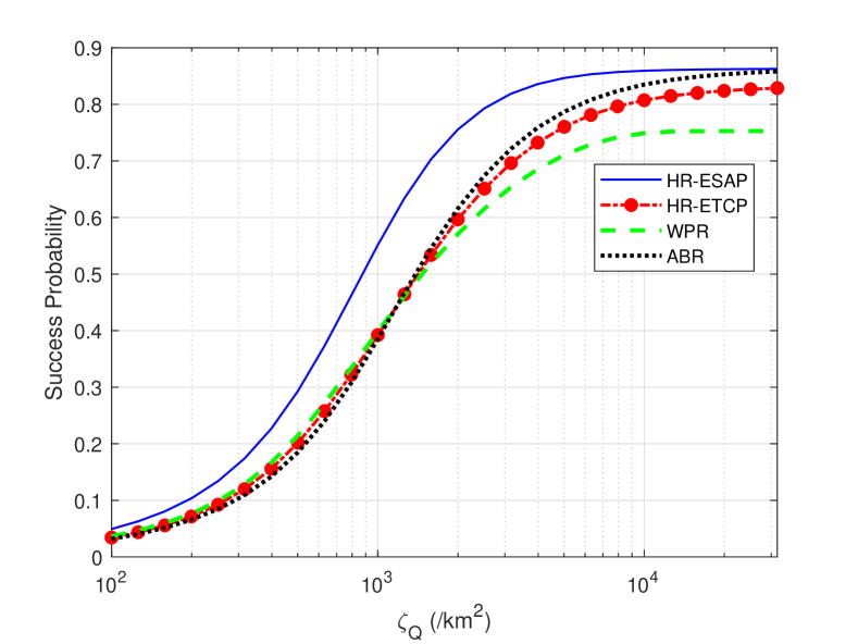
Figure 6: Success probability as a function of $\widetilde{\zeta}$.

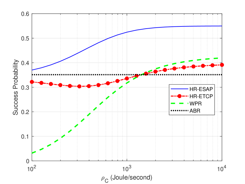
Figure 7: Success probability as a function of $\rho_{C}$.

VI-3 Impact of Normalized Capacitor Capacity $\rho_{C}$ on Success Probability

In Fig. 7, we investigate the impact of the normalized capacitor capacity i.e., $\rho_{C}=\frac{E_{C}}{T}$. It can be found that the capacity of the capacitor has a considerable impact on the success probabilities of the hybrid relaying with ESAP and the pure WPR. The reason is that the capacitor capacity is directly related to the transmit power of the wireless-powered transmission. By contrast, $\mathcal{S}_{\textup{ABR}}$ remains steady with the variation of $\rho_{C}$, as the transmit power of the pure ABR is not related to the capacitor capacity. As $\mathcal{S}_{\textup{ABR}}$ outperforms $\mathcal{S}_{\textup{WPR}}$ in most of the shown range, $\mathcal{S}^{\textup{ETCP}}_{\textup{HR}}$ approaches $\mathcal{S}_{\textup{ABR}}$ closely due to the exploration process, and thus less affected by $\rho_{C}$ compared to $\mathcal{S}^{\textup{ESAP}}_{\textup{HR}}$ and $\mathcal{S}_{\textup{WPR}}$. We note that both the success probabilities of the hybrid relaying with ESAP and the pure WPR are saturated when $\varrho_{C}$ becomes large. This implies that it is not necessary to equip an capacitor with oversized capacity for the hybrid relaying and the pure WPR. In practice, the capacitor capacity can be properly chosen to achieve a certain objective of success probability in the target network environment. Furthermore, by integrating ambient backscattering, the hybrid relaying with either ESAP or ETCP can relieve the requirement on capacitor capacity compared with the pure WPR.

VI-4 Effect of Energy Harvesting Time Fraction $\omega$ on Ergodic Capacity

Fig. 9 examines the impact of the energy harvesting time fraction $\omega$ of the relaying protocol on the ergodic capacity performance. We first validate the analytical expressions of $\mathcal{C}^{\textup{ESAP}}_{\textup{HR}}$, $\mathcal{C}^{\textup{ETCP}}_{\textup{HR}}$, $\mathcal{C}_{\textup{ABR}}$, and $\mathcal{C}_{\textup{WPR}}$ obtained in Theorem 3, Theorem 4, Corollary 3, and Corollary 4, respectively. It can be seen that our analytical results of ergodic capacity well match the Monte Carlo simulation results over a wide range of $\omega$. In terms of the ergodic capacity, the hybrid relaying with ESAP still achieves the higher ergodic capacity than those of the pure ABR and the pure WPR. We can observe that the plots of the hybrid relaying with ESAP and the pure WPR are unimodal functions of $\omega$ within the shown range. This reveals that there can be an optimal value of $\omega$ to maximize the ergodic capacity of the hybrid relaying and the pure WPR. It is noted that the ergodic capacity of the pure ABR is also a unimodal function of $\omega$. Due to the ultra-lower circuit power consumption, the maximal $\mathcal{C}_{\textup{ABR}}$ is achieved at a value much smaller than the shown range, and thus we omit displaying it. Moreover, the performance gap between the hybrid relaying with ESAP and the pure WPR becomes larger with the decrease of the energy harvesting time fraction. This implies that the smaller the energy harvesting time, the greater the performance gain of the hybrid relaying with ESAP over the pure WPR. The reason is that ABR is adopted when the harvested energy is deficient for active transmission, which largely lowers the demand for capacitor compared to the pure WPR.

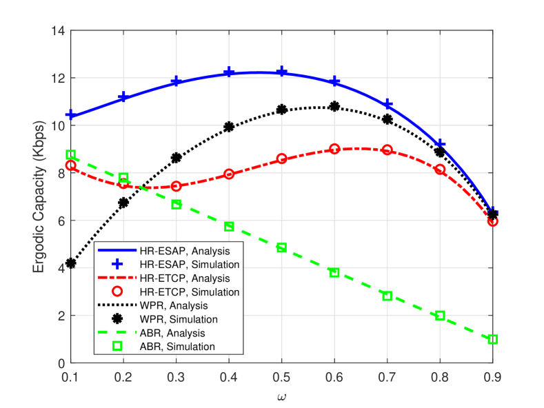
Figure 8: Success probability as a function of the energy harvesting time fraction $\omega$.

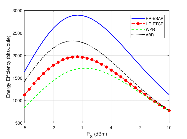
Figure 9: Energy efficiency as a function of $P_{\mathrm{S}}$ ($\tau_{\mathrm{A}}=10\tau_{\mathrm{A}}$).

VI-5 Impact of Transmit Power $P_{\mathrm{S}}$ on Energy Efficiency

Based on the analytical results of ergodic capacity, we also evaluate the energy efficiency of the relaying system, defined as the ergodic capacity versus the transmit power of the source node, i.e., $\mathcal{E}_{\textup{HR}}=\frac{\mathcal{C}_{\textup{HR}}}{P_{\mathrm{S}}}$. As shown in Fig. LABEL:fig:EE_PS, the ergodic capacities of all types of the relaying are unimodal functions of $P_{\mathrm{S}}$. Specifically, increasing $P_{\mathrm{S}}$ at first enhances the energy efficiency because of an increase of the ergodic capacity. However, as $P_{\mathrm{S}}$ keeps increasing, it becomes more dominant than the ergodic capacity which consequently deteriorates the energy efficiency. It can also be observed that the maximum energy efficiencies for different types of the relaying are achieved at different values of $P_{\mathrm{S}}$. The reason is that the energy efficiency depends not only on $P_{\mathrm{S}}$, but also $\omega$ which determines the amount of harvesting energy of $\mathrm{R}$ and the transmission time of each hop. Thus, other than $P_{\mathrm{S}}$, $\omega$ is also another key design parameter to improve the energy efficiency.

VI-6 Applications of Analytical Framework

Furthermore, we demonstrate applications of the derived analytical framework in optimizing system parameters. In energy-constrained communication systems, power allocation is a crucial design issue. Therefore, we consider two power allocation-related design problems: transmit power minimization and energy efficiency maximization. For the first problem, we minimize the transmit power of the source node with constraints on the minimum capacity in order to optimize the energy harvesting time fraction $\omega$. The formulation is expressed as follows:

$$\mathbf{P1}:\hskip 8.53581pt\min_{\omega}\quad\quad P_{\mathrm{S}}$$

$$\begin{array}[]{r@{\quad}r@{}l@{\quad}l}\text{subject to}&\quad\mathbf{C1}:\quad\mathcal{C}_{\textup{HR}}\hskip 2.84526pt\geq\hskip 2.84526pt\mathcal{C}^{\textup{Target}}_{\textup{HR}},&\\ &\mathbf{C2}:\hskip 8.53581pt0\hskip 2.84526pt\leq\hskip 2.84526ptP_{\mathrm{S}}\leq\hskip 2.84526pt\bar{P},&\hskip 8.53581pt0\hskip 2.84526pt\leq\hskip 2.84526ptP^{\mathrm{W}}_{\mathrm{R}}\hskip 2.84526pt\leq\hskip 2.84526pt\bar{P},\\ &\mathbf{C3}:\hskip 9.95845pt0\hskip 2.84526pt\leq\hskip 2.84526pt\omega\hskip 2.84526pt\leq\hskip 2.84526pt1.&\\ \end{array}$$

where $\mathcal{C}^{\textup{Target}}_{\textup{HR}}$ denotes the target ergodic capacity and $\bar{P}$ denotes the maximum transmit power for the source node and the relay node in the WPR mode. $\mathbf{C2}$ denotes the transmit power constraints for the source node and the hybrid relay, and $\mathbf{C3}$ denotes the time allocation constraint.

For the second problem, we maximize the energy efficiency of the relaying system with the reliability constraint that the success probability of the hybrid relaying should be above some target value, denoted as $\mathcal{S}^{\textup{Target}}_{\textup{HR}}$. The formulation is shown as follows:

$$\mathbf{P2}:\hskip 8.53581pt\max_{\omega,P_{\mathrm{S}}}\quad\quad\mathcal{E}_{\textup{HR}}=\frac{\mathcal{C}_{\textup{HR}}}{P_{\mathrm{S}}}$$

$$\begin{array}[]{r@{\quad}r@{}l@{\quad}l}\text{subject to}&\quad\mathbf{C1}:\quad\mathcal{S}_{\textup{HR}}\hskip 2.84526pt\geq\hskip 2.84526pt\mathcal{S}^{\textup{Target}}_{\textup{HR}},&\\ &\mathbf{C2}:\hskip 8.53581pt0\hskip 2.84526pt\leq\hskip 2.84526ptP_{\mathrm{S}}\leq\hskip 2.84526pt\bar{P},&\hskip 8.53581pt0\hskip 2.84526pt\leq\hskip 2.84526ptP^{\mathrm{W}}_{\mathrm{R}}\hskip 2.84526pt\leq\hskip 2.84526pt\bar{P},\\ &\mathbf{C3}:\hskip 9.6739pt0\hskip 2.84526pt\leq\hskip 2.84526pt\omega\hskip 2.84526pt\leq\hskip 2.84526pt1.&\\ \end{array}$$

where $\mathbf{C1}$ is the reliability requirement and $\mathbf{C2}$ and $\mathbf{C3}$ are the same as those in $\mathbf{P1}$. Solving this problem provides us optimal choices of the energy harvesting time fraction $\omega$ and transmit power $P_{\mathrm{S}}$.

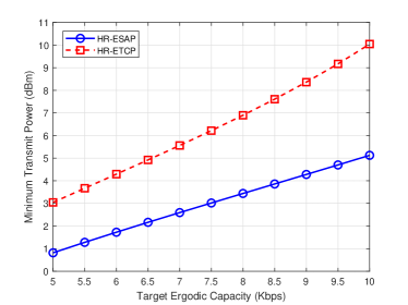
(a) Maximum energy efficiency as a function of target success probability.

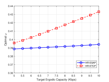
(b) Optimal energy harvesting time fraction as a function of target success probability.

Figure 10: Optimal energy harvesting time fraction and maximum energy efficiency with reliability constraints. ($\rho_{Q}=2000/$km², $\bar{P}=25$ dBm)

VI-7 Numerical Solutions of Optimization Problems

Next, we numerically solve the formulated optimization problems. Fig. 10(a) and Fig. 10(b) illustrates the minimum transmit power allocation and corresponding energy harvesting time allocation as functions of the target ergodic capacity, respectively, for $\mathbf{P1}$. As expected, the minimum transmit power is an increasing function of the target ergodic capacity. By utilizing the instantaneous CSI, the hybrid relaying with ESAP achieves the same target ergodic capacity with much lower transmit power than that with ETCP. Minimizing the transmit power has a larger impact on the optimal solutions of $\omega$ for the hybrid relaying with ETCP than that with ESAP.

Fig. 11(a) and Fig.11(b) demonstrate the maximum energy efficiency and the corresponding energy harvesting time allocation as functions of the target success probability, respectively, for $\mathbf{P2}$. Again, the hybrid relaying with ESAP outperforms that with ETCP in terms of maximum energy efficiency due to higher achieved capacity. It is observed that with the increase of the target success probability the maximum energy efficiency first remains steady and then decreases. The reason is that larger $P_{\mathrm{S}}$ is required to ensure higher reliability, which may sacrifice the energy efficiency. Moreover, the optimal $\omega$ increases with the reliability requirement. This can be understood straightforwardly that more harvested energy is needed for the hybrid relay to perform WPR in order to guarantee a high reliability. The results of the optimal resource allocation problem can be used as guidance for setting the hybrid relaying to balance the tradeoff between energy efficiency and the reliability.

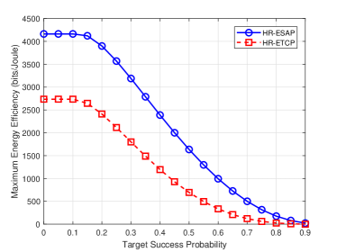
(a) Maximum energy efficiency as a function of target success probability.

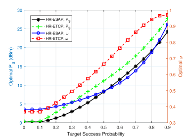
(b) Optimal energy harvesting time fraction as a function of target success probability.

Figure 11: Optimal energy harvesting time fraction and maximum energy efficiency with reliability constraints. ($\rho_{Q}=2000/$km², $\bar{P}=30$ dBm)

VII Conclusion

We have proposed a hybrid relaying paradigm that is capable of operating in either ambient backscatter relaying mode or wireless-powered relaying mode. Both relaying modes are based on, but have different ways of utilizing ambient RF signals. Therefore, how to switch between the two relaying modes under different network environment largely determines the performance of the hybrid relaying. To address this issue, we have devised two protocols for the hybrid relaying to perform operational mode selection with and without instantaneous CSI. Considering the use of the hybrid relaying in a dual-hop relay system with spatially randomly located ambient transmitters, we have derived the end-to-end success probabilities and ergodic capacity of the system under different mode selection protocols based on stochastic geometry analysis. We have demonstrated analytically and numerically the superiority of the hybrid relaying over the pure wireless-powered relaying and the pure ambient backscatter relaying, as the proposed mode selection protocols effectively select the proper operation to adapt to the system environment. The analytical results reveal the impacts of different system parameters on the studied performance metrics and allow us to optimize the system parameters based on the objective. Our analytical framework can be extended to investigate intelligent reconfigurable surface [55, 56] assisted relaying. Another promising direction is to design online learning (e.g., bandit learning [57]) based mode selection protocol for the hybrid relaying.

Appendix

VII-A Proof of Theorem 1

Proof.

According to the criteria of ESAP described in Section II, we have the probability that the hybrid relay being in the WPR mode and the ABR mode, respectively, expressed as

$$\mathbb{P}\big{[}\mathrm{M}_{\textup{ESAP}}=\mathrm{W}\big{]}=\mathbb{P}\Big{[}\nu_{\mathrm{R}}\!>\!\tau_{\mathrm{W}},E_{\mathrm{R}}\!>\!E_{\mathrm{W}},\nu^{\mathrm{W}}_{\mathrm{D}}\!>\!\tau_{\mathrm{W}}\Big{]},$$ (33)

and $$\mathbb{P}\big{[}\mathrm{M}_{\textup{ESAP}}=\mathrm{A}\big{]}=\mathbb{P}\Big{[}\nu_{\mathrm{R}}\!>\!\tau_{\mathrm{W}},E_{\mathrm{R}}\!>\!E_{\mathrm{W}},\nu^{\mathrm{W}}_{\mathrm{D}}\!\leq\!\tau_{\mathrm{W}}\Big{]}+\mathbb{P}\Big{[}E_{\mathrm{W}}\!\geq\!E_{\mathrm{R}}\!>\!E_{\mathrm{A}}\Big{]}.$$ (34)

By inserting (33) and (34) into (IV), we have

$$\mathcal{S}^{\textup{ESAP}}_{\textup{HR}}=\!\underbrace{\mathbb{P}\Big{[}\nu_{\mathrm{R}}\!>\!\tau_{\mathrm{W}},\nu^{\mathrm{W}}_{\mathrm{D}}\!>\!\tau_{\mathrm{W}},E_{\mathrm{R}}\!>\!E_{\mathrm{W}}\Big{]}}_{\mathcal{S}^{\textup{ESAP}}_{\mathrm{W}}}\!$$

$$\hskip 42.67912pt+\underbrace{\mathbb{P}\Big{[}\nu_{\mathrm{R}}\!>\!\tau_{\mathrm{W}},\nu^{\mathrm{A}}_{\mathrm{D}}\!>\!\tau_{\mathrm{A}},\nu^{\mathrm{W}}_{\mathrm{D}}\!\leq\!\tau_{\mathrm{W}},E_{\mathrm{R}}\!>\!E_{\mathrm{W}}\Big{]}+\mathbb{P}\Big{[}\nu_{\mathrm{R}}\!>\!\tau_{\mathrm{W}},\nu^{\mathrm{A}}_{\mathrm{D}}\!>\!\tau_{\mathrm{A}},E_{\mathrm{W}}\!\geq\!E_{\mathrm{R}}\!>\!E_{\mathrm{A}}\Big{]}}_{\mathcal{S}^{\textup{ESAP}}_{\mathrm{A}}},$$ (35)

where $\mathcal{S}^{\textup{ESAP}}_{\mathrm{W}}$ ($\mathcal{S}^{\textup{ESAP}}_{\mathrm{A}}$) represents the joint probability that the transmission is successful and the hybrid relay is in the WPR (ABR) mode under ESAP. We first obtain $\mathcal{S}^{\textup{ESAP}}_{\mathrm{W}}$ as follows:

$$\mathcal{S}^{\textup{ESAP}}_{\mathrm{W}}\!\!=\mathbb{P}\bigg{[}h_{\mathrm{S},\mathrm{R}}>\frac{d^{\mu}_{\mathrm{S},\mathrm{R}}\tau_{\mathrm{W}}(I_{\mathrm{R}}\!+\!\sigma^{2})}{P_{\mathrm{S}}},h_{\mathrm{R},\mathrm{D}}>\frac{d^{\mu}_{\mathrm{R},\mathrm{D}}\tau_{\mathrm{W}}(I_{\mathrm{D}}\!+\!\sigma^{2})}{P^{\mathrm{W}}_{\mathrm{R}}},\omega\beta TQ_{\mathrm{R}}>E_{\mathrm{W}}\bigg{]}$$

$$\!\!\overset{\text{(a)}}{=}\mathbb{E}\bigg{[}\exp\!\bigg{(}\!\!-\!\frac{d^{\mu}_{\mathrm{S},\mathrm{R}}\tau_{\mathrm{W}}}{P_{\mathrm{S}}}\Big{(}\!\sum_{j\in\Phi}\!\!\frac{P_{T}h_{j,\mathrm{R}}}{d^{\mu}_{j,\mathrm{R}}}\!+\!\sigma^{2}\!\Big{)}\!\!\bigg{)}\exp\!\bigg{(}\!\!-\!\frac{d^{\mu}_{\mathrm{R},\mathrm{D}}\tau_{\mathrm{W}}}{P^{\mathrm{W}}_{\mathrm{R}}}\Big{(}\!\sum_{j\in\Phi}\!\!\frac{P_{T}h_{j,\mathrm{D}}}{d^{\mu}_{j,\mathrm{D}}}\!+\!\sigma^{2}\!\Big{)}\!\!\bigg{)}{\bf 1}_{\{Q_{\mathrm{R}}>\varrho_{\mathrm{W}}\}}\bigg{]}$$

$$\!\!\overset{\text{(b)}}{=}\exp\!\Big{(}\!\!-\!\kappa(\tau_{\mathrm{W}})\sigma^{2}\!\Big{)}\!\Bigg{(}\!\!\exp\!\Big{(}\!\!-\!\ell(\tau_{\mathrm{W}},\rho_{C})\sigma^{2}\!\Big{)}\mathbb{E}_{\Phi}\!\Bigg{[}\prod_{j\in\Phi}\!\Big{(}\!1\!+\!\frac{\kappa(\tau_{\mathrm{W}})P_{T}}{d^{\mu}_{j,\mathrm{R}}}\Big{)}^{\!\!\!-1}\!\Big{(}\!1\!+\!\frac{\ell(\tau_{\mathrm{W}},\rho_{C})P_{T}}{d^{\mu}_{j,\mathrm{D}}}\Big{)}^{\!\!-1}\!\Bigg{]}\!\!\int^{\infty}_{\!\!\varrho_{\mathrm{W}}+\varrho_{C}}\!\!\!\!\!f_{Q_{\mathrm{R}}}(q)\mathrm{d}q$$

$$\!\!\hskip 5.69054pt+\!\!\int^{\varrho_{\mathrm{W}}+\varrho_{C}}_{\varrho_{\mathrm{W}}}\!\!\!\exp\!\Big{(}\!\!-\!\ell(\tau_{\mathrm{W}},\omega\beta q-\rho_{\mathrm{W}})\sigma^{2}\!\Big{)}\mathbb{E}_{\Phi}\Bigg{[}\prod_{j\in\Phi}\!\Big{(}\!1\!+\!\frac{\kappa(\tau_{\mathrm{W}})P_{T}}{d^{\mu}_{j,\mathrm{R}}}\!\Big{)}^{\!\!\!-1}\!\Big{(}\!1\!+\!\frac{\ell(\tau_{\mathrm{W}},\omega\beta q-\rho_{\mathrm{W}})P_{T}}{d^{\mu}_{j,\mathrm{R}}}\!\Big{)}^{\!\!-1}\!\Bigg{]}f_{Q_{\mathrm{R}}}(q)\mathrm{d}q\!$$

$$\!\!\overset{\text{(c)}}{=}\exp\!\big{(}\!-\!\kappa(\tau_{\mathrm{W}})\sigma^{2}\big{)}\!\Bigg{(}\!\exp\!\Big{(}\!\!-\!\ell(\tau_{\mathrm{W}},\rho_{C})\sigma^{2}\!\Big{)}\mathrm{Det}\Big{(}\mathrm{Id}\!+\!\alpha\mathbb{G}_{\Phi}(\mathbf{x},\mathbf{y})\varphi_{\mathbf{x}}\big{(}\ell(\tau_{\mathrm{W}},\rho_{C})\big{)}\varphi_{\mathbf{y}}\big{(}\ell(\tau_{\mathrm{W}},\rho_{C})\big{)}\!\Big{)}^{\!-\frac{1}{\alpha}}$$

$$\times\!\Big{(}1\!-\!F_{Q_{\mathrm{R}}}\big{(}\varrho_{\mathrm{W}}\!+\!\varrho_{C}\big{)}\!\Big{)}\!+\!\!\int^{\varrho_{\mathrm{W}}+\varrho_{\mathrm{C}}}_{\!\varrho_{\mathrm{W}}}\!\!\!\mathrm{Det}\Big{(}\mathrm{Id}\!+\!\alpha\mathbb{G}_{\Phi}(\mathbf{x},\mathbf{y})\varphi_{\mathbf{x}}\big{(}\ell(\tau_{\mathrm{W}},\omega\beta q\!-\!\rho_{\mathrm{W}})\varphi_{\mathbf{y}}\big{(}\ell(\tau_{\mathrm{W}},\omega\beta q\!-\!\rho_{\mathrm{W}})\big{)}\!\Big{)}^{\!\!-\frac{1}{\alpha}}$$

$$\hskip 241.84842pt\times\exp\!\Big{(}\!\!-\!\ell(\tau_{\mathrm{W}},\omega\beta q-\rho_{\mathrm{W}})\sigma^{2}\!\Big{)}f_{Q_{\mathrm{R}}}(q)\mathrm{d}q\!\Bigg{)},\!\!$$ (36)

where (a) follows the complementary CDF of the exponential random variable, i.e., $\mathbb{P}[h>x]=\exp(-x)$ for $h\sim\exp(1)$, (b) follows the Laplace transform of an exponential random variable, i.e., $\mathcal{L}_{h}(Z)=(1+Z)^{-1}$ for $h\sim\exp(1)$ and applies the substitutions $\kappa(v)=\frac{d^{\mu}_{\mathrm{S},\mathrm{R}}v}{P_{\mathrm{S}}}$ and $\ell(v,p)=\!\frac{d^{\mu}_{\mathrm{R},\mathrm{D}}v(1-\omega)}{2p}$, and (c) applies Theorem $1$ of [36].

Subsequently, we continue to derive $\mathcal{S}^{\textup{ESAP}}_{\mathrm{A}}$ as follows:

$$\mathcal{S}^{\textup{ESAP}}_{\mathrm{A}}=\mathbb{P}\bigg{[}h_{\mathrm{S},\mathrm{R}}\!>\!\frac{d^{\mu}_{\mathrm{S},\mathrm{R}}\tau_{\mathrm{W}}(I_{\mathrm{R}}\!+\!\sigma^{2})}{P_{\mathrm{S}}},\widetilde{h}_{\mathrm{R},\mathrm{D}}\!>\!\frac{d^{\mu}_{\mathrm{R},\mathrm{D}}\widetilde{\sigma}^{2}\tau_{\mathrm{A}}}{\eta\xi Q_{\mathrm{R}}},h_{\mathrm{R},\mathrm{D}}\!\leq\!\frac{d^{\mu}_{\mathrm{R},\mathrm{D}}\tau_{\mathrm{W}}(I_{\mathrm{D}}\!+\!\sigma^{2})}{P^{\mathrm{W}}_{\mathrm{R}}},\omega\beta TQ_{\mathrm{R}}\!>\!Q_{\mathrm{W}}\bigg{]}$$

$$\hskip 142.26378pt+\mathbb{P}\bigg{[}h_{\mathrm{S},\mathrm{R}}\!>\!\frac{\tau_{\mathrm{W}}d^{\mu}_{\mathrm{S},\mathrm{R}}(I_{\mathrm{R}}\!+\!\sigma^{2})}{P_{\mathrm{S}}},\widetilde{h}_{\mathrm{R},\mathrm{D}}\!>\!\frac{d^{\mu}_{\mathrm{R},\mathrm{D}}\widetilde{\sigma}^{2}\tau_{\mathrm{A}}}{\eta\xi Q_{\mathrm{R}}},E_{\mathrm{W}}\!\geq\!\omega\beta TQ_{\mathrm{R}}\!>\!E_{\mathrm{A}}\bigg{]}.$$

$$\overset{\text{(d)}}{=}\exp\!\big{(}\!-\!\kappa(\tau_{\mathrm{W}})\sigma^{2}\big{)}\!\bigg{(}\!\mathrm{Det}\Big{(}\mathrm{Id}\!+\!\alpha\mathbb{G}_{\Phi}(\mathbf{x},\mathbf{y})\psi_{\mathbf{x}}\big{(}\kappa(\tau_{\mathrm{W}})\big{)}\psi_{\mathbf{y}}\big{(}\kappa(\tau_{\mathrm{W}})\big{)}\!\Big{)}^{\!\!-\!\frac{1}{\alpha}}\!\!\!\int^{\infty}_{\varrho_{\mathrm{A}}}\!\!\delta(q)f_{Q_{\mathrm{R}}}(q)\mathrm{d}q\!$$

$$\hskip 85.35826pt-\chi_{\mathbb{A}}(\tau_{\mathrm{W}},\rho_{C})\!\int^{\infty}_{\varrho_{\mathrm{W}}+\varrho_{C}}\!\!\!\delta(q)f_{Q_{\mathrm{R}}}(q)\mathrm{d}q-\!\int^{\varrho_{\mathrm{W}}\!+\!\varrho_{C}}_{\varrho_{\mathrm{W}}}\!\!\!\chi_{\mathbb{A}}(\tau_{\mathrm{W}},\omega\beta q\!-\!\rho_{\mathrm{W}})\delta(q)\!f_{Q_{\mathrm{R}}}(q)\mathrm{d}q\!\bigg{)}.$$ (37)

where (d) follows similar derivation steps of $\mathcal{S}^{\textup{ESAP}}_{\mathrm{W}}$ in (36) and $\chi_{\mathbb{A}}(v,p)$ has been defined in (12).

Finally, by plugging (36) and (37) into (35), we have $\mathcal{S}^{\textup{ESAP}}_{\textup{HR}}$ expressed in (1). ∎

VII-B Proof of Corollary 2

Proof.

The case when the ambient emitters and interferers are distributed following PPPs can be modeled as a special case of our adopted $\alpha$-GPP when $\alpha\to\infty$. In particular, by using the expansion [50]

$$\mathrm{Det}\big{(}\mathrm{Id}+\alpha\mathbb{B}_{\Phi}(s)\big{)}^{-\frac{1}{\alpha}}\stackrel{{\scriptstyle\alpha\to 0}}{{\longrightarrow}}\exp\left(-\int_{\mathbb{O}}\mathbb{B}_{\Phi}(\mathbf{x},\mathbf{x})\mathrm{d}\mathbf{x}\right),$$ (38)

we can simplify the Fredholm determinant in (13) as follows when $\alpha\to\infty$, $\widetilde{\alpha}\to\infty$, and $\mu=4$:

$$\mathrm{Det}\Big{(}\mathrm{Id}\!+\!\alpha\mathbb{B}_{\Phi}\big{(}\kappa(\tau_{\mathrm{W}})\big{)}\!\Big{)}^{-\frac{1}{\alpha}} \!=\!\exp\!\left(\!-2\pi\zeta\int^{R\to\infty}_{0}\!\bigg{(}1-\Big{(}1\!+\!\frac{d^{4}_{\mathrm{S},\mathrm{R}}\tau_{\mathrm{W}}P_{T}}{P_{\mathrm{S}}r^{4}}\Big{)}^{-1}\bigg{)}r\mathrm{d}r\right)$$

$$=\exp\left(\!-\frac{1}{2}\pi^{2}\zeta\sqrt{\frac{d^{4}_{\mathrm{S},\mathrm{R}}\tau_{\mathrm{W}}P_{T}}{P_{\mathrm{S}}}}\right).$$ (39)

Similarly, following the expansion in (38), $f_{Q_{\mathrm{R}}}$(q) can be simplified as follows:

$$f_{Q_{\mathrm{R}}}(q) \!=\!\mathcal{L}^{-1}\!\left\{\exp\!\left[-2\pi\widetilde{\zeta}\!\int^{R\to\infty}_{0}\!\!\frac{r}{1\!+\!r^{4}(s\widetilde{P}_{T})^{-1}}\mathrm{d}r\right]\right\}(q)=\mathcal{L}^{-1}\!\left\{\exp\left(\!-\frac{\pi^{2}}{2}\widetilde{\zeta}\sqrt{s\widetilde{P}_{T}}\right)\!\right\}(q)$$

$$\overset{\text{(e)}}{=}\frac{1}{2\pi i}\lim_{T\to\infty}\int^{C+iT}_{C-iT}\exp\left(qs\right)\exp\left(\!-\frac{\pi^{2}}{2}\widetilde{\zeta}\sqrt{s\widetilde{P}_{T}}\right)\mathrm{d}s$$

$$\overset{\text{(f)}}{=}\frac{1}{\pi}\int^{\infty}_{0}\exp(-qt)\left[\frac{\exp\Big{(}\frac{i}{2}\pi^{2}\widetilde{\zeta}\sqrt{t\widetilde{P}_{T}}\Big{)}-\exp\Big{(}\!-\!\frac{i}{2}\pi^{2}\widetilde{\zeta}\sqrt{t\widetilde{P}_{T}}\Big{)}}{2i}\right]\mathrm{d}t$$

$$\overset{\text{(g)}}{=}\frac{1}{\pi}\int^{\infty}_{0}\exp(-qt)\sin\Big{(}\frac{1}{2}\pi^{2}\widetilde{\zeta}\sqrt{t\widetilde{P}_{T}}\Big{)}\mathrm{d}u=\frac{1}{4}\left(\frac{\pi}{q}\right)^{\!\!\frac{3}{2}}\widetilde{\zeta}\sqrt{\widetilde{P}_{T}}\exp\left(-\frac{\pi^{4}\widetilde{\zeta}^{2}\widetilde{P}_{T}}{16q}\right),$$ (40)

where (e) follows from Mellin’s inverse formula [42] which transforms the inverse Laplace transform into the complex plane, and $C$ is a fixed constant greater than the real parts of the singularities of $\exp\left(\!-\frac{\pi^{2}}{2}\widetilde{\zeta}\sqrt{s\widetilde{P}_{T}}\right)$, (f) applies the Bromwich inversion theorem with the modified contour, and (g) holds as $\frac{\exp(ix)-\exp(-ix)}{2i}=\sin(x)$.

Finally, by plugging (39) and (40) into (13), we can obtain $\mathcal{S}_{\textup{ABR}}$ in (18) after some mathematical manipulations. ∎

VII-C Proof of Theorem 2

Proof.

With ETCP, the mode selection of $\mathrm{R}$ is based on achieved performance in previous time slots instead of the current one. Therefore, the steady-state success probability of the hybrid relaying in a certain mode is independent of the mode selection probability. Recall that the hybrid relay under ETCP eventually selects the ABR mode when the number of successful transmission in the ABR mode is higher than that in the WPR mode during the exploration period. According to this mode selection criteria, the corresponding success probability can be expressed as

$$\mathcal{S}^{\textup{ETCP}}_{\textup{HR}}\!=\!\mathbb{P}\Big{[}\nu_{\mathrm{R}}\!>\!\tau_{\mathrm{W}},\nu^{\mathrm{W}}_{\mathrm{D}}\!>\!\tau_{\mathrm{W}},E_{\mathrm{R}}\!>\!E_{\mathrm{W}}\Big{]}\mathbb{P}\Big{[}\mathrm{M}_{\textup{ETCP}}\!=\!\mathrm{W}\Big{]}\!+\!\mathbb{P}\Big{[}\nu_{\mathrm{R}}\!>\!\tau_{\mathrm{W}},\nu^{\mathrm{A}}_{\mathrm{D}}\!>\!\tau_{\mathrm{A}},E_{\mathrm{R}}\!>\!E_{\mathrm{A}}\Big{]}\mathbb{P}\Big{[}\mathrm{M}_{\textup{ETCP}}\!=\!\mathrm{A}\Big{]}$$

$$+\!\frac{1}{2}\bigg{(}\!1\!-\!\mathbb{P}\Big{[}\nu_{\mathrm{R}}\!>\!\tau_{\mathrm{W}},\nu^{\mathrm{W}}_{\mathrm{D}}\!>\!\tau_{\mathrm{W}},E_{\mathrm{R}}\!>\!E_{\mathrm{W}}\Big{]}\!-\mathbb{P}\Big{[}\nu_{\mathrm{R}}\!>\!\tau_{\mathrm{W}},\nu^{\mathrm{A}}_{\mathrm{D}}\!>\!\tau_{\mathrm{A}},E_{\mathrm{R}}\!>\!E_{\mathrm{A}}\Big{]}\!\bigg{)}\!\bigg{(}\!\mathbb{P}\Big{[}\mathrm{M}_{\textup{ETCP}}\!=\!\mathrm{W}\Big{]}\!\!+\!\mathbb{P}\Big{[}\mathrm{M}_{\textup{ETCP}}\!=\!\mathrm{A}\Big{]}\!\bigg{)}$$

$$=\frac{1}{2}(\mathcal{S}_{\textup{WPR}}+\mathcal{S}_{\textup{ABR}})+\frac{1}{2}\bigg{(}\mathbb{P}\Big{[}N_{\textup{WPR}}\!>\!N_{\textup{ABR}}\Big{]}-\mathbb{P}\Big{[}N_{\textup{ABR}}\!>\!N_{\textup{WPR}}\Big{]}\bigg{)}(\mathcal{S}_{\textup{WPR}}-\mathcal{S}_{\textup{ABR}}).$$ (41)

The number of successful transmissions in the ABR mode and that in the WPR mode are dependent on $\mathcal{S}_{\textup{ABR}}$ and $\mathcal{S}_{\textup{WPR}}$, obtained in (13) and (19), respectively. Based on these results, we have

$$\mathbb{P}\big{[}N_{\textup{ABR}}\!>\!N_{\textup{WPR}}\big{]}=\sum^{n}_{i=1}{n\choose i}\mathbb{P}\big{[}N_{\textup{ABR}}=i\big{]}\sum^{i}_{j=1}{n\choose i\!-\!j}\mathbb{P}\big{[}N_{\textup{WPR}}=i-j\big{]}$$

$$=\sum^{n}_{i=1}{n\choose i}\mathcal{S}^{i}_{\textup{ABR}}(1-\mathcal{S}_{\textup{ABR}})^{n-i}\sum^{i}_{j=1}{n\choose i-j}\mathcal{S}^{i-j}_{\textup{WPR}}\big{(}1-\mathcal{S}_{\textup{WPR}}\big{)}^{n-i+j}.$$ (42)

Similarly, we have

$$\mathbb{P}\big{[}N_{\textup{WPR}}\!>\!N_{\textup{ABR}}\big{]}=\sum^{n}_{i=1}{n\choose i}\mathcal{S}^{i}_{\textup{WPR}}(1-\mathcal{S}_{\textup{WPR}})^{n-i}\sum^{i}_{j=1}{n\choose i\!-\!j}\mathcal{S}^{i-j}_{\textup{ABR}}\big{(}1-\mathcal{S}_{\textup{ABR}}\big{)}^{n-i+j}.$$ (43)

Then, by inserting (VII-C) and (43) into (VII-C), we have the expression of $\mathcal{S}^{\textup{ETCP}}_{\textup{HR}}$ in (22). ∎

VII-D Proof of Theorem 3

Proof.

Recall that, with ESAP, the probabilities of the hybrid relaying working in the WPR mode (i.e., $\mathbb{P}[\mathrm{M}=\mathrm{W}]$) and ambient backscatter mode (i.e., $\mathbb{P}[\mathrm{M}=\mathrm{A}]$) have been obtained in (33) and (34), respectively. By inserting (33) and (34) into the definition in (V), we have the ergodic capacity of the hybrid relaying with ESAP as follows:

$$\mathcal{C}^{\textup{ESAP}}_{\textup{HR}} =\frac{1-\omega}{2}\Bigg{(}\mathbb{E}\Big{[}W\log_{2}(1+\nu){\bf 1}_{\{\nu_{\mathrm{R}}>\tau_{\mathrm{W}},\nu^{\mathrm{W}}_{\mathrm{D}}>\tau_{\mathrm{W}},E_{\mathrm{R}}>E_{\mathrm{W}}\}}\Big{]}+C_{\mathrm{A}}\bigg{(}\mathbb{P}\Big{[}\nu_{\mathrm{R}}\!>\!\tau_{\mathrm{W}},\nu^{\mathrm{A}}_{\mathrm{D}}\!>\!\tau_{\mathrm{A}},\nu^{\mathrm{W}}_{\mathrm{D}}\!\leq\!\tau_{\mathrm{W}},E_{\mathrm{R}}\!>\!E_{\mathrm{W}}\Big{]}$$

$$\hskip 256.0748pt+\mathbb{P}\Big{[}\nu_{\mathrm{R}}\!>\!\tau_{\mathrm{W}},\nu^{\mathrm{A}}_{\mathrm{D}}\!>\!\tau_{\mathrm{A}},E_{\mathrm{W}}\!\geq\!E_{\mathrm{R}}>E_{\mathrm{A}}\Big{]}\bigg{)}\!\Bigg{)}$$

$$=\frac{1-\omega}{2}\bigg{(}\mathbb{E}\Big{[}W\log_{2}(1+\nu){\bf 1}_{\{\nu_{\mathrm{R}}>\tau_{\mathrm{W}},\nu^{\mathrm{W}}_{\mathrm{D}}>\tau_{\mathrm{W}},E_{\mathrm{R}}>E_{\mathrm{W}}\}}\Big{]}+C_{\mathrm{A}}\mathcal{S}^{\textup{ESAP}}_{\mathrm{A}}\!\bigg{)},$$ (44)

where $\mathcal{S}^{\textup{ESAP}}_{\mathrm{A}}$ has been obtained in (37).

The first term in the brackets of (44) can be calculated as

$$\mathbb{E}\Big{[}W\log_{2}(1+\nu){\bf 1}_{\{\nu_{\mathrm{R}}>\tau_{\mathrm{W}},\nu^{\mathrm{W}}_{\mathrm{D}}>\tau_{\mathrm{W}},E_{\mathrm{R}}>E_{\mathrm{W}}\}}\Big{]}\overset{\text{(h)}}{=}W\!\int^{\infty}_{0}\!\mathbb{P}\Big{[}\log_{2}(1+\nu){\bf 1}_{\{\nu_{\mathrm{R}}>\tau_{\mathrm{W}},\nu^{\mathrm{W}}_{\mathrm{D}}>\tau_{\mathrm{W}},E_{\mathrm{R}}>E_{\mathrm{W}}\}}>t\Big{]}\mathrm{d}t$$

$$\overset{\text{(i)}}{=}\frac{W}{\ln(2)}\!\int^{\infty}_{0}\!\mathbb{P}\Big{[}\nu>v,\omega T\beta Q_{\mathrm{R}}\!>\!E_{\mathrm{W}}\Big{]}\frac{1}{1+v}\mathrm{d}v=\frac{W}{\ln(2)}\!\int^{\infty}_{0}\!\mathbb{P}\Big{[}\min(\nu_{\mathrm{R}},\nu^{\mathrm{W}}_{\mathrm{D}})>v,Q_{\mathrm{R}}>\varrho_{\mathrm{W}}\Big{]}\frac{1}{1+v}\mathrm{d}v$$

$$=\frac{W}{\ln(2)}\!\int^{\infty}_{0}\!\mathbb{P}\Big{[}\nu_{\mathrm{R}}>v,\nu^{\mathrm{W}}_{\mathrm{D}}>v,Q_{\mathrm{R}}>\varrho_{\mathrm{W}}\Big{]}\frac{1}{1+v}\mathrm{d}v$$

$$\overset{\text{(j)}}{=}\!\frac{W}{\ln(2)}\!\int^{\infty}_{0}\!\exp\!\Big{(}\!\!-\!\kappa(v)\sigma^{2}\!\Big{)}\!\bigg{(}\!\chi_{\mathbb{A}}(\tau_{\mathrm{W}},\rho_{C})\Big{(}1\!-\!F_{Q_{\mathrm{R}}}(\varrho_{\mathrm{W}}\!+\!\varrho_{C})\!\Big{)}$$

$$\hskip 241.84842pt+\!\int^{\varrho_{\mathrm{W}}\!+\!\varrho_{C}}_{\varrho_{\mathrm{W}}}\!\!\!\!\chi_{\mathbb{A}}(\tau_{\mathrm{W}},\omega\beta q\!-\!\rho_{\mathrm{W}})f_{Q_{\mathrm{R}}}(q)\mathrm{d}q\!\bigg{)}\frac{1}{1+v}\mathrm{d}v,$$ (45)

where (h) follows $\mathbb{E}[A]=\int^{\infty}_{0}\mathbb{P}[A>t]\mathrm{d}t$ [51], (i) replaces $t$ with $\log_{2}(1+v)$, and (j) follows the derivation of $\mathcal{S}^{\textup{ESAP}}_{\mathrm{W}}$ in (36) with $\tau_{\mathrm{W}}$ replaced by $v$.

Then, by plugging (37) and (45) into (44), we have the ergodic capacity of the hybrid relaying with ESAP in (24). ∎

References

• [1] X. Lu, G. Li, H. Jiang, D. Niyato, and P. Wang, “Performance analysis of wireless-powered relaying with ambient backscattering,” in Proc. of IEEE ICC, Kansas City, MO, USA, May 2018.
• [2] Q. Wu, M. Tao, Derrick Wing Kwan Ng, W. Chen, and R. Schober, “Energy-efficient resource allocation for wireless powered communication networks,” IEEE Trans. Wireless Commun., vol. 15, no. 3, pp. 2312-2327, Nov. 2015.
• [3] H. Lee, K.-J. Lee, H. Kim, B. Clerckx, and I. Lee, “Resource allocation techniques for wireless powered communication networks with capacitor constraint,” IEEE Transactions on Wireless Communications, vol. 15, no. 4, pp. 2619-2628, Apr. 2016.
• [4] Q. Wu, W. Chen, Derrick Wing Kwan Ng, and R. Schober, “User-centric energy efficiency maximization for wireless powered communications,” IEEE Trans. Wireless Commun., vol. 15, no. 10, pp. 6898-6912, Jul. 2016.
• [5] E. Boshkovska, and D. W. K. Ng, and N. Zlatanov, and A. Koelpin, and R. Schober, “Robust resource allocation for MIMO wireless powered communication networks based on a non-linear EH model,” IEEE Transactions on Communications, vol. 65, no. 5, pp. 1984-1999, May 2017.
• [6] D. Niyato, X. Lu, P. Wang, D. I. Kim, and Z. Han, “Distributed wireless energy scheduling for wireless powered sensor networks,” IEEE International Conference on Communications, Kuala Lumpur, Malaysia, May 2016.
• [7] S. Bi, Y. Zeng, R. Zhang, “Wireless powered communication networks: An overview,” IEEE Wireless Communications, vol. 23, no. 2, pp, 10-18, Apr. 2016.
• [8] X. Lu, P. Wang, D. Niyato, D. I. Kim, and Z. Han, “Wireless charger networking for mobile devices: Fundamentals, standards, and applications,” IEEE Wireless Communications, vol. 22, no. 2, pp. 126-135, 2015.
• [9] D. Niyato, X. Lu, P. Wang, D. I. Kim, and Z. Han, “Economics of Internet of things (IoT): An information market approach,” IEEE Wireless Communications, vol. 23, no. 4, Aug. 2016.
• [10] W. Y. Toh, Y. K. Tan, W. S. Koh, and L. Siek, “Autonomous wearable sensor nodes with flexible energy harvesting,” IEEE Sensors Journal, vol. 14, no. 7, pp. 2299-2306, Jul. 2014.
• [11] X. Lu, P. Wang, and D. Niyato, “A layered coalitional game framework of wireless relay network,” IEEE Transactions on Vehicular Technology, vol. 63, no. 1, pp. 472-478, Jan. 2014.
• [12] Y. Zeng and R. Zhang, “Full-duplex wireless-powered relay with self-energy recycling,” IEEE Wireless Communications Letters, vol. 4, no. 2, pp. 201-204, Apr. 2015.
• [13] Y. Zeng, H. Chen, and R. Zhang, “Bidirectional wireless information and power transfer with a helping relay,” IEEE Communications Letters, vol. 20, no. 5, pp. 862-865, May 2016.
• [14] L. Tang, X. Zhang, P. Zhu, and X. Wang “Wireless information and energy transfer in fading relay channels,” IEEE Journal on Selected Areas in Communications, vol. 34, no. 12, pp. 3632-3645, Dec. 2016.
• [15] Z. Chen, L. X. Cai, Y. Cheng, and H. Shan, “ Sustainable cooperative communication in wireless powered networks with energy harvesting relay,” IEEE Transactions on Wireless Communications, vol. 16, no. 12, pp. 8175-8189, Dec. 2017.
• [16] V. Liu, A. Parks, V. Talla, S. Gollakota, D. Wetherall, and J. R. Smith, “Ambient backscatter: Wireless communication out of thin air,” in Proc. of ACM SIGCOMM, Aug. 2013.
• [17] X. Lu, P. Wang, D. Niyato, D. I. Kim, and Z. Han, “Wireless networks with RF energy harvesting: A contemporary survey,” IEEE Commun. Surveys Tuts., vol. 17, no. 2, pp. 757–789, 2nd Quart., 2015.
• [18] H. Chen, Y. Li, J. L. Rebelatto, B. F. Uchôa-Filho, and B. Vucetic, “Harvest-then-cooperate: wireless-powered cooperative communications,” IEEE Transactions on Signal Processing, vol. 63, no. 7, pp. 1700-1711, Apr. 2015.
• [19] X. Lu, D. Niyato, H. Jiang, D. I. Kim, Y. Xiao and Z. Han, “Ambient backscatter assisted wireless powered communications”, IEEE Wireless Communications, vol. 25, no. 2, pp. 170-177, Apr. 2018.
• [20] A. N. Parks et al., “Turbocharging ambient backscatter communication,” in prod. of the 2014 ACM conference on SIGCOMM, Chicago, IL, Aug. 2014.
• [21] N. V. Huynh, D. T. Hoang, X. Lu, D. Niyato, P. Wang, and D. I. Kim, “Ambient backscatter communications: A contemporary survey,” to appear IEEE Communications Surveys $\&$ Tutorials.
• [22] D. T. Hoang, D. Niyato, P. Wang, D. I. Kim, and Z. Han, “Ambient backscatter: A new approach to improve network performance for RF-powered cognitive radio networks,” vol. 65, no. 9, pp. 3659-3674, Sept. 2017.
• [23] L. Decreusefond, I. Flint, and A. Vergne, “A note on the simulation of the Ginibre point process,” J. Appl. Probab., vol. 52, no. 4, pp. 1003-1012, Dec. 2015.
• [24] I. Flint, X. Lu, N. Privault, D. Niyato, and P. Wang, “Performance analysis of ambient RF energy harvesting: A stochastic geometry approach,” IEEE Global Telecommunications Conference, Austin, TX, Dec. 2014.
• [25] X. Lu, I. Flint, D. Niyato, N. Privault, and P. Wang, “Performance analysis of simultaneous wireless information and power transfer with ambient RF energy harvesting,” IEEE Wireless Communications and Networking Conference, New Orleans, LA, March 2015.
• [26] X. Lu, I. Flint, D. Niyato, N. Privault and P. Wang, “Self-sustainable communications with RF energy harvesting: Ginibre point process modeling and analysis,” Journal on Selected Areas in Communications (JSAC), vol. 34, no. 5, pp. 1518-1535, May 2016.
• [27] I. Flint, et al., “Performance analysis of ambient RF energy harvesting with repulsive point process modelling,” IEEE Transactions on Wireless Communications, vol. 14, no. 10, pp. 5402-5416, May 2015.
• [28] M. Z. Win, P. C. Pinto, and L. A. Shepp, “A mathematical theory of network interference and its applications,” Proceedings of the IEEE, vol. 97, no. 2, pp. 205-230, Feb. 2009.
• [29] P. Hu, P. Zhang, M. Rostami, and D. Ganesan, “Braidio: An integrated active-passive radio for mobile devices with asymmetric energy budgets,” in proc. of ACM SIGCOMM, Florianopolis, Brazil, Aug. 2016.
• [30] V. A. Aalo, G. P. Efthymoglou, T. Soithong, M. Alwakeel, and S. Alwakeel, “Performance analysis of multi-hop amplify-and-forward Relaying systems in Rayleigh fading channels with a Poisson interference field,” IEEE Transactions on Wireless Communications, vol. 13, no. 1, pp. 24-35, Jan. 2014.
• [31] A. A. Nasir, X. Zhou, S. Durrani, and R. A. Kennedy, “Relaying protocols for wireless energy harvesting and information processing,” IEEE Trans. Wireless Commun., vol. 12, no. 7, pp. 3622-3636, Jul. 2013.
• [32] A. A. Nasir, X. Zhou, S. Durrani, and R. A. Kennedy, “Wireless-powered relays in cooperative communications: Time-switching relaying protocols and throughput analysis,” IEEE Transactions on Communications, vol. 63, no. 5, pp. 1607-1622, May 2015.
• [33] X. Lu, P. Wang, D. Niyato, D. I. Kim, and Z. Han, “Wireless networks with RF energy harvesting: A contemporary survey,” IEEE Communications Surveys and Tutorials, vol. 17, no. 2, pp. 757-789, May 2015.
• [34] K. Huang, E. Larsson, “Simultaneous information and power transfer for broadband wireless systems,” IEEE Transactions on Signal Processing, vol. 61, no. 23, pp. 5972-5986, Dec. 2013.
• [35] I. Krikidis, “Simultaneous information and energy transfer in large-scale networks with/without relaying,” IEEE Transactions on Communications, vol. 62, no. 3, pp. 900-912, Mar. 2014.
• [36] L. Decreusefond et al., “Determinantal point processes,” in Stochastic Analysis for Poisson Point Processes, Springer, pp. 311-342, Jun. 2016.
• [37] C. Boyer and S. Roy, “Coded QAM backscatter modulation for RFID,” IEEE Transactions on Communications, vol. 60, pp. 1925-1934, Jul. 2012.
• [38] S. Gurucharya, X. Lu, E. Hossain, “Optimal non-coherent detector for ambient backscatter communication system,” IEEE Transactions on Vehicular Technology, vol. 69, no. 12, pp. 16197 - 16201, Dec. 2020.
• [39] C. Boyer, and S. Roy, “Backscatter communication and RFID: Coding, energy, and MIMO analysis,” IEEE Transactions on Communications, vol. 62, no. 3, pp. 770-785, Mar. 2014.
• [40] D.-Y. Kim, H.-G. Yoon, B.-J. Jang, and J.-G. Yook, “Effects of reader-to-reader interference on the UHF RFID interrogation range,” IEEE Transactions on Industrial Electronics, vol. 56, no. 7, pp. 2337-2346, Jul. 2009.
• [41] J. Kimionis, A. Bletsas, and J. N. Sahalos, “Bistatic backscatter radio for tag read-range extension,” in Proc. of IEEE International Conference on RFID-Technologies and Applications (RFID-TA), Nice, France, Nov. 2012.
• [42] P. Flajolet, et al “Mellin transforms and asymptotics: Harmonic sums,” Theoretical Computer Science, vol. 144, no. 1-2, pp. 3-58, Jun. 1995.
• [43] G. Li, P. Zhao, X. Lu, J. Liu, and Y. Shen, “Data analytics for fog computing by distributed online learning with asynchronous update,” IEEE International Conference on Communications (ICC), Shanghai, China, May 2019.
• [44] G. Li, Y. Shen, P. Zhao, X. Lu, J. Liu, Y. Liu, and S. C. Hoi, “Detecting cyberattacks in industrial control systems using online learning algorithms,” Neurocomputing, vol. 364, pp. 338-348, 2019.
• [45] R. B. Ash, Basic Probability Theory, Dover, 2008.
• [46] X. Lu, H. Jiang, D. Niyato, D. I. Kim and Z. Han, “Wireless-powered device-to-device communications with ambient backscattering: Performance modeling and analysis,” IEEE Transactions on Wireless Communications, vol. 17, no. 3, pp. 1528-1544, Mar. 2018.
• [47] H.-B. Kong, et al “Exact performance analysis of ambient RF energy harvesting wireless sensor networks with Ginibre point process,” IEEE Journal on Selected Areas in Communications, vol. 34, no. 12, pp. 3769-3784, Dec. 2016.
• [48] H.-B. Kong, P. Wang, D. Niyato, and Y. Cheng, “Modeling and analysis of wireless sensor networks using Ginibre point processes,” IEEE Transactions on Wireless Communications, vol. 16, no. 6, pp. 3700-3713, Jun. 2017.
• [49] M. Abramowitz and I. A. Stegun, Handbook of mathematical functions with formulas, graphs, mathematical tables, 9th ed. New York, NY, USA: Dover, 1972.
• [50] T. Shirai and Y. Takahashi, “Random point fields associated with certain Fredholm determinants I: Fermion, Poisson and Boson point processes,” Journal of Functional Analysis, vol. 205, no. 2, pp. 414-463, Dec. 2003.
• [51] J. G. Andrews, F. Baccelli, and R. K. Ganti, “A tractable approach to coverage and rate in cellular networks,” IEEE Transactions on Communications, vol. 59, no. 11, pp. 3122-3134, Nov. 2011.
• [52] B. Kellogg, A. Parks, S. Gollakota, J. R. Smith, and D. Wetherall, “Wi-Fi backscatter: Internet connectivity for RF-powered devices,” ACM SIGCOMM Computer Communication Review, vol. 44, no. 4, pp. 607-618, August 2014.
• [53] C. Gomez, and J. Paradells, “Wireless home automation networks: A survey of architectures and technologies,” IEEE Communications Magazine, vol. 48, no. 6, pp. 92-101, June 2010.
• [54] X. Lu, P. Wang, D. Niyato, D. I. Kim and Z. Han, “Wireless charging technologies: Fundamentals, standards, and network applications,” IEEE Communications Surveys and Tutorials, vol. 18, no. 2, pp. 1413-1452, Second Quarter, 2016.
• [55] X. Lu, E. Hossain, T. Shafique, S. Feng, H. Jiang, and D. Niyato, “Intelligent reflecting surface enabled covert communications in wireless networks,” IEEE Network, vol. 34, no. 5, pp. 148-155, June 2020.
• [56] S. Gong, X. Lu, D. T. Hoang, D. Niyato, L. Shu, D. I. Kim, and Y. C. Liang, “Toward smart wireless communications via intelligent reflecting surfaces: A contemporary survey IEEE Communications Surveys & Tutorials, vol. 22, no. 4, pp. 2283-2314, Fourthquarter 2020.
• [57] G. Li, X. Lu, and D. Niyato, “A bandit approach for mode selection in ambient backscatter-assisted wireless-powered relaying,” IEEE Transactions on Vehicular Technology, vol. 69, no. 8, Aug. 2020.