Stability and Generalization of the Decentralized Stochastic Gradient Descent

Abstract

The stability and generalization of stochastic gradient-based methods provide valuable insights into understanding the algorithmic performance of machine learning models. As the main workhorse for deep learning, stochastic gradient descent has received a considerable amount of studies. Nevertheless, the community paid little attention to its decentralized variants. In this paper, we provide a novel formulation of the decentralized stochastic gradient descent. Leveraging this formulation together with (non)convex optimization theory, we establish the first stability and generalization guarantees for the decentralized stochastic gradient descent. Our theoretical results are built on top of a few common and mild assumptions and reveal that the decentralization deteriorates the stability of SGD for the first time. We verify our theoretical findings by using a variety of decentralized settings and benchmark machine learning models.

Introduction

The great success of deep learning (LeCun, Bengio, and Hinton 2015) gives impetus to the development of stochastic gradient descent (SGD) (Robbins and Monro 1951) and its variants (Nemirovski et al. 2009; Duchi, Hazan, and Singer 2011; Rakhlin, Shamir, and Sridharan 2012; Kingma and Ba 2014; Wang et al. 2020). Although the convergence results of SGD are abundant, the effects caused by the training data is absent. To this end, the generalization error (Hardt, Recht, and Singer 2016; Lin, Camoriano, and Rosasco 2016; Bousquet and Elisseeff 2002; Bottou and Bousquet 2008) is developed as an alternative method to analyze SGD. The generalization bound reveals the performance of stochastic algorithms and characterizes how the training data and stochastic algorithm jointly affect the target machine learning model. To mathematically describe generalization, Hardt, Recht, and Singer (2016); Bousquet and Elisseeff (2002); Elisseeff, Evgeniou, and Pontil (2005) introduce the algorithmic stability for SGD, which mainly depends on the landscape of the underlying loss function, to study the generalization bound of SGD. The stability theory of SGD has been further developed (Charles and Papailiopoulos 2018; Kuzborskij and Lampert 2018; Lei and Ying 2020).

SGD has already been widely used in parallel and distributed settings (Agarwal and Duchi 2011; Dekel et al. 2012; Recht et al. 2011), e.g., the decentralized SGD (D-SGD) (Ram, Nedić, and Veeravalli 2010b; Lan, Lee, and Zhou 2020; Srivastava and Nedic 2011; Lian et al. 2017). D-SGD is implemented without a centralized parameter server, and all nodes are connected through an undirected graph. Compared to the centralized SGD, the decentralized one requires much less communication with the busiest node (Lian et al. 2017), accelerating the whole computational system.

From the theoretical viewpoint, although there exist plenty of convergence analysis of D-SGD (Sirb and Ye 2016; Lan, Lee, and Zhou 2020; Lian et al. 2017, 2018), the stability and generalization analysis of D-SGD remains rare.

Contributions

In this paper, we establish the first theoretical result on the stability and generalization of the D-SGD. We elaborate on our contributions below.

1. Stability of D-SGD: We provide the uniform stability of D-SGD in the general convex, strongly convex, and nonconvex cases. Our theory shows that besides the learning rate, data size, and iteration number, the stability and generalization of D-SGD are also dependent on the connected graph structure. To the best of our knowledge, our result is the first theoretical stability guarantee for D-SGD. In the general convex setting, we also present the stability of D-SGD in terms of the ergodic average instead of the last iteration for the excess generalization analysis.

2. Computational errors for D-SGD with convexity and projection: We consider more general schemes of D-SGD, that is, D-SGD with projection. In the previous work (Ram, Nedić, and Veeravalli 2010b), to get the convergence rate, the authors need to make additional assumptions on the graph ([Assumptions 2 and 3, (Ram, Nedić, and Veeravalli 2010b)]). In this paper, we remove these assumptions, and we present the computational errors of D-SGD with projections in the strongly convex setting.

3. Generalization bounds for D-SGD with convexity: We derive (excess) generalization bounds for convex D-SGD. The excess generalization is controlled by the computational error and the generalization bound, which can be directly obtained from the stability.

4. Numerical results: We numerically verify our theoretical results by using various benchmark machine learning models, ranging from strongly convex and convex to nonconvex settings, in different decentralized settings.

Prior Art

In this section, we briefly review two kinds of related works: decentralized optimization and stability and generalization analysis of SGD.

Decentralized and distributed optimization Decentralized algorithms arise in calculating the mean of data distributed over multiple sensors (Boyd et al. 2005; Olfati-Saber, Fax, and Murray 2007). The decentralized (sub)gradient descent (DGD) algorithms are propose and studied by (Nedic and Ozdaglar 2009; Yuan, Ling, and Yin 2016). Recently, DGD has been generalized to the stochastic settings. With a local Poisson clock assumption on each agent, Ram, Nedić, and Veeravalli (2010a) proposes an asynchronous gossip algorithm. The decentralized algorithm with a random communication graph is proposed in (Srivastava and Nedic 2011; Ram, Nedić, and Veeravalli 2010b). Sirb and Ye (2016); Lan, Lee, and Zhou (2020); Lian et al. (2017) consider the randomness caused by the stochastic gradients and proposed the decentralized SGD (D-SGD). The complexity analysis of D-SGD has been done in (Sirb and Ye 2016). In (Lan, Lee, and Zhou 2020), the authors propose another kind of D-SGD that leverages dual information, and provide the related computational complexity. In the paper (Lian et al. 2017), the authors show the advantage of D-SGD compared to the centralized SGD. In a recent paper (Lian et al. 2018), the authors developed asynchronous D-SGD with theoretical convergence guarantees. The biased decentralized SGD is proposed and studied by (Sun et al. 2019). In (Richards and others 2020), the authors studied the stability for a non-fully decentralized training method, in which each node needs to communicate extra gradient information. Paper (Richards and others 2020) is closed to ours, but we consider the DSGD, which is different from the algorithm investigated by (Richards and others 2020) and more general. Further more, we studied the nonconvex settings.

Stability and Generalization of SGD In (Shalev-Shwartz et al. 2010), on-average stability is proposed and further studied by Kuzborskij and Lampert (2018). The uniform stability of empirical risk minimization (ERM) under strongly convex objectives is considered by Bousquet and Elisseeff (2002). Extended results are proved with the pointwise-hypothesis assumption, which shows that a class of learning algorithms is convergent with global optimum (Charles and Papailiopoulos 2018). In order to prove uniform stability of SGD, Hardt, Recht, and Singer (2016) reformulate SGD as a contractive iteration. In (Lei and Ying 2020), a new stability notion is proposed to remove the bounded gradient assumptions. In (Bottou and Bousquet 2008), the authors establish a framework for the generalization performance of SGD. Hardt, Recht, and Singer (2016) connects the uniform stability with generalization error. The generalization errors with strong convexity are established in (Hardt, Recht, and Singer 2016; Lin, Camoriano, and Rosasco 2016). The stability and generalization are also studied for the Langevin dynamics (Li, Luo, and Qiao 2019; Mou et al. 2018).

Setup

This part contains preliminaries and mathematical descriptions of our problem. Analyzing the stability of D-SGD is more complicated than that of SGD due to the challenge arises from the mixing matrix in D-SGD. We cannot directly adapt the analysis for SGD to D-SGD. To this end, we reformulate D-SGD as an operator iteration with an error term, which is followed by bounding the error in each iteration.

Stability and Generalization

The population risk minimization is an important model in machine learning and statistics, whose mathematical formulation reads as

$$\min_{{\bf x}\in\mathbb{R}^{d}}R({\bf x}):=\mathbb{E}_{\xi\sim\mathcal{D}}f({\bf x};\xi),$$

where $f({\bf x};\xi)$ denotes the loss of the model associated with data $\xi$ and $\mathcal{D}$ is the data distribution. Due to the fact that $\mathcal{D}$ is usually unknown or very complicated, we consider the following surrogate ERM

$$\min_{{\bf x}\in\mathbb{R}^{d}}R_{S}({\bf x}):=\frac{1}{N}\sum_{i=1}^{N}f({\bf x};\xi_{i}),$$

where $S:=\{\xi_{1},\xi_{2},\ldots,\xi_{N}\}$ and $~{}\xi_{i}\sim\mathcal{D}$ is a given data.

For a specific stochastic algorithm $\mathcal{A}$ act on $S$ with output $\mathcal{A}(S)$, the generalization error of $\mathcal{A}$ is defined as $\epsilon_{\textrm{gen}}:=\mathbb{E}_{S,\mathcal{A}}[R(\mathcal{A}(S))-R_{S}(\mathcal{A}(S))].$ Here, the expectation is taken over the algorithm and the data. The generalization bound reflects the joint effects caused by the data $S$ and the algorithm $\mathcal{A}$. We are also interested in the excess generalization error, which is defined as $\epsilon_{\textrm{ex-gen}}:=\mathbb{E}_{S,\mathcal{A}}[R(\mathcal{A}(S))-R({\bf x}^{*})]$, where ${\bf x}^{*}$ is the minimizer of $R$. Let $\overline{{\bf x}}$ be the minimizer of $R_{S}$. Due to the unbiased expectation of the data $S$, we have $\mathbb{E}_{S}[R_{S}({\bf x}^{*})]=\mathbb{E}[R({\bf x}^{*})]$. Thus, Bottou and Bousquet (2008) point out $\epsilon_{\textrm{ex-gen}}$ can be decomposed as follows

$$\mathbb{E}_{S,\mathcal{A}}[R(\mathcal{A}(S))-R({\bf x}^{*})]=\underbrace{\mathbb{E}_{S,\mathcal{A}}[R(\mathcal{A}(S))-R_{S}(\mathcal{A}(S))]}_{\textrm{generalization error}}$$

$$+\underbrace{\mathbb{E}_{S,\mathcal{A}}[R_{S}(\mathcal{A}(S))-R_{S}(\overline{{\bf x}})]}_{\textrm{optimization error}}+\underbrace{\mathbb{E}_{S,\mathcal{A}}[R_{S}(\overline{{\bf x}})-R_{S}({\bf x}^{*})]}_{\textrm{test error}}.$$

Notice that $R_{S}(\overline{{\bf x}})\leq R_{S}({\bf x}^{*})$, therefore

$$\epsilon_{\textrm{ex-gen}}\leq\epsilon_{\textrm{gen}}+\mathbb{E}_{S,\mathcal{A}}[R_{S}(\mathcal{A}(S))-R_{S}(\overline{{\bf x}})].$$

The uniform stability is used to bound the generalization error of a given algorithm $\mathcal{A}$ (Hardt, Recht, and Singer 2016; Elisseeff, Evgeniou, and Pontil 2005).

Definition 1

We say that the randomized algorithm $\mathcal{A}$ is $\epsilon$-uniformly stable if for any two data sets $S,S^{\prime}$ with $n$ samples that differ in one example, we have

$$\sup_{\xi}\mathbb{E}_{\mathcal{A}}\left[f(\mathcal{A}(S);\xi)-f(\mathcal{A}(S^{\prime});\xi)\right]\leq\epsilon.$$

It has been proved that the uniform stability directly implies the generalization bound.

Lemma 1 ((Hardt, Recht, and Singer 2016))

Let $\mathcal{A}$ be $\epsilon$-uniformly stable, it follows $|\mathbb{E}_{S,\mathcal{A}}[R(\mathcal{A}(S))-R_{S}(\mathcal{A}(S))]|\leq\epsilon.$

Thus, to get the generalization bound of a random algorithm, we just need to compute the uniform stability bound $\epsilon$.

Problem Formulation

Notation: We use the following notations throughout the paper. We denote the $\ell_{2}$ norm of ${\bf x}\in\mathbb{R}^{d}$ as $\|{\bf x}\|$. For a matrix ${\bf A}$, ${\bf A}^{\top}$ denotes its transpose, we denote the spectral norm of ${\bf A}$ as $\|{\bf A}\|_{\textrm{op}}$. Given another matrix ${\bf B}$, ${\bf A}\succ{\bf B}$ means that ${\bf A}-{\bf B}$ is positive define; and ${\bf A}\succeq{\bf B}$ means ${\bf A}-{\bf B}$ is positive semidefinite. The identity matrix is defined as $\mathbb{I}$. We use $\mathbb{E}[\cdot]$ to denote the expectation of $\cdot$ with respect to the underlying probability space. For two positive constants $a$ and $b$, we denote $a=\mathcal{O}(b)$ if there exists $C>0$ such that $a\leq Cb$, and $\widetilde{\mathcal{O}}(b)$ hides a logarithmic factor of $b$.

Let $\mathcal{D}_{i}=\{\xi_{l(i)}\}_{1\leq l\leq n}$ ($1\leq i\leq m$) denote the data stored in the $i$th client, which follow the same distribution of $\mathcal{D}$ . In this paper, we consider solving the objective function  (1) by the DGD, where

$$f({\bf x}):=\frac{1}{mn}\sum_{i=1}^{m}\sum_{l=1}^{n}f({\bf x};\xi_{l(i)}).$$ (1)

Note that (1) is a decentralized approximation to the following population risk function

$$F({\bf x}):=\mathbb{E}_{\xi\sim\mathcal{D}}f({\bf x};\xi).$$ (2)

To distinguish from the objective functions in the last subsection, we use $f$ rather than $R_{S}$ here. The decentralized optimization is usually associated with a mixing matrix, which is designed by the users according to a given graph structure. In particular, we consider the connected graph $\mathcal{G}=(\mathcal{V},\mathcal{E})$ with vertex set $\mathcal{V}=\{1,...,M\}$ and edge set $\mathcal{E}\subseteq\mathcal{V}\times\mathcal{V}$ with edge $(i,l)\in\mathcal{E}$ represents the communication link between nodes $i$ and $l$. Before proceeding, let us recall the definition of the mixing matrix.

Definition 2 (Mixing matrix)

For any given graph $\mathcal{G}=(\mathcal{V},\mathcal{E})$, the mixing matrix ${\bf W}=[w_{ij}]\in\mathbb{R}^{M\times M}$ is defined on the edge set $\mathcal{V}$ that satisfies: (1) If $i\neq j$ and $(i,j)\notin{\cal E}$, then $w_{ij}=0$; otherwise, $w_{ij}>0$; (2) ${\bf W}={\bf W}^{\top}$; (3) $\mathrm{null}\{\mathbb{I}-{\bf W}\}=\mathrm{span}\{\bf 1\}$; (4) $\mathbb{I}\succeq{\bf W}\succ-\mathbb{I}.$

Note that ${\bf W}$ is a doubly stochastic matrix (Marshall, Olkin, and Arnold 1979), and the mixing matrix is non-unique for a given graph. Several common examples for ${\bf W}$ include the Laplacian matrix and the maximum-degree matrix (Boyd, Diaconis, and Xiao 2004). A crucial constant that characterizes the mixing matrix is

$$\lambda:=\max\{|\lambda_{2}|,|\lambda_{m}({\bf W})|\},$$

where $\lambda_{i}$ denotes the $i$th largest eigenvalue of ${\bf W}\in\mathbb{R}^{m\times m}$. The definition of the mixing matrix implies that $0\leq\lambda<1$.

Lemma 2 (Corollary 1.14., (Montenegro and Tetali 2006))

Let ${\bf P}\in\mathbb{R}^{m\times m}$ be the matrix whose elements are all $1/m$. Given any $k\in\mathbb{Z}^{+}$, the mixing matrix ${\bf W}\in\mathbb{R}^{m\times m}$ satisfies

$$\|{\bf W}^{k}-{\bf P}\|_{\emph{op}}\leq\lambda^{k}.$$

Note the fact that the stationary distribution of an irreducible aperiodic finite Markov chain is uniform if and only if its transition matrix is doubly stochastic. Thus, ${\bf W}$ corresponds to some Markov chain’s transition matrix, and the parameter $0\leq\lambda<1$ characterizes the speed of convergence to the stationary state.

We consider a general decentralized stochastic gradient descent with projection, which carries out in the following manner: in the $t$-th iteration, 1) client $i$ applies an approximate copy ${\bf x}^{t}(i)\in\mathbb{R}^{d}$ to calculate a unbiased gradient estimate $\nabla f({\bf x}^{t}(i);\xi_{j_{t}(i)})$, where $j_{t}(i)\in\mathbb{Z}^{+}$ is the local random index; 2) client $i$ replaces its local parameters with the weighted average of its neighbors, i.e.,

$$\tilde{{\bf x}}^{t}(i)=\sum_{l\in\mathcal{N}(i)}w_{i,l}{\bf x}^{t}(l);$$ (3)

3) client $i$ updates its parameters as

$${\bf x}^{t+1}(i) =\textbf{Proj}_{V}\Big{(}\tilde{{\bf x}}^{t}(i)-\alpha_{t}\nabla f({\bf x}^{t}(i);\xi_{j_{t}(i)})\Big{)}$$ (4)

with learning rate $\alpha_{t}>0$, and ${\bf Proj}_{V}(\cdot)$ stands for projecting the quantity $\cdot$ into the space $V$. We stress that, in practice, we do not need to compute the average ${\bf x}^{t}=\frac{1}{m}\sum_{i=1}^{m}{\bf x}^{t}(i)$ in each iteration, and we take the average only in the last iteration.

Algorithm 1 Decentralized Stochastic Gradient Descent (D-SGD)

0:  $(\alpha_{t}>0)_{t\geq 0}$, initialization ${\bf x}^{0}$for node $i=1,2,\ldots,m$   for $t=1,2,\ldots$     updates local parameter as (3) and (4)    ${\bf x}^{t}=\frac{1}{m}\sum_{i=1}^{m}{\bf x}^{t}(i)$  end forend for

In the following, we draw necessary assumptions, which are all common and widely used in the nonconvex analysis community.

Assumption 1

The loss function $f({\bf x};\xi)$ is nonnegative and differentiable with respect to ${\bf x}$, and $\nabla f({\bf x};\xi)$ is bounded by the constant $B$ over $V$, i.e., $\max_{{\bf x}\in V,\xi\sim\mathcal{D}}\|\nabla f({\bf x};\xi)\|\leq B$.

Assumption 1 implies that $|f({\bf x};\xi)-f({\bf y};\xi)|\leq B\|{\bf x}-{\bf y}\|,$ for all ${\bf x},{\bf y}\in V$ and any $\xi\sim\mathcal{D}$.

Assumption 2

The gradient of $f({\bf x};\xi)$ with respect to ${\bf x}$ is $L$-Lipschitz, i.e., $\|\nabla f({\bf x};\xi)-\nabla f({\bf y};\xi)\|\leq L\|{\bf x}-{\bf y}\|,$ for all ${\bf x},{\bf y}\in V$ and any $\xi\sim\mathcal{D}$.

Assumption 3

The set $V$ forms a closed ball in $\mathbb{R}^{d}$.

Compared with the scheme presented in (Lian et al. 2017), our algorithm accommodates a projection after each update in each client. When $\nabla f({\bf x};\xi)$ is non-strongly convex, $V$ can be set as the full space and Algorithm 1 reduces to the scheme given in (Lian et al. 2017), whose convergence has been well studied. Such a projection is more general and is necessary for the strongly convex analysis; we explain this necessary claim as follows: if $f$ is $\nu$-strongly convex, then $\|\nabla f({\bf x})\|^{2}\geq\nu\|{\bf x}-{\bf x}^{*}\|^{2}$ with ${\bf x}^{*}$ being the minimizer of $f({\bf x})$ (Karimi, Nutini, and Schmidt 2016). Thus, when ${\bf x}$ is far from ${\bf x}^{*}$, the gradient is unbounded, which breaks Assumption 1. However, with the projection procedure, D-SGD (Algorithm 1) actually minimizes function (1) over the set $V$. The strong convexity gives us $f({\bf x})-f({\bf x}^{*})\geq\frac{\nu}{2}\|{\bf x}-{\bf x}^{*}\|^{2}$, which indicates ${\bf x}^{*}\in\textbf{B}(\textbf{0},\sqrt{{2(f({\bf x}^{0})-\min f)}/{\nu}})$. Thus, when the radius of $V$ is large enough, the projection does not change the output of D-SGD.

Stability of D-SGD

In this section, we prove the stability theory for D-SGD in strongly convex, convex, and nonconvex settings.

General Convexity

This part contains the stability result of D-SGD when $f(\cdot;\xi)$ is generally convex.

Theorem 1

Let $f(\cdot;\xi)$ be convex and Assumptions 1, 2, 3 hold. If the step size $\alpha_{t}\leq{2}/{L}$, then D-SGD satisfies the uniform stability with

$$\epsilon_{\emph{stab}}\leq\frac{2B^{2}\sum_{t=1}^{T-1}\alpha_{t}}{mn}+4B^{2}\sum_{t=1}^{T-1}\Big{[}(1+\alpha_{t}B)\sum_{j=0}^{t-1}\alpha_{j}\lambda^{t-1-j}\Big{]}.$$

Compared to the results of minimizing (1) by using centralized SGD with step sizes $(\alpha_{t})_{t\geq 1}$ [Theorem 3.8, (Hardt, Recht, and Singer 2016)], which yields the uniformly stable bound as ${2B^{2}\sum_{t=1}^{T-1}\alpha_{t}}/{(mn)}$. Theorem 1 shows that D-SGD suffers from an additional term $4B^{2}\sum_{t=1}^{T-1}(1+\alpha_{t}B)\sum_{j=0}^{t-1}\alpha_{j}\lambda^{t-1-j}$, which does not vanish when $\lambda>0$.

If we set $\alpha_{t}={1}/{(t+1)}$, with Lemma 3, it is easy to check that $\epsilon_{\textrm{stab}}=\mathcal{O}(\frac{\ln T}{mn}+C_{\lambda}\ln T)$; However, if we use a constant learning rate, (i.e., $\alpha_{t}\equiv\alpha$), when $0<\lambda<1$, we have $4B^{2}\sum_{t=1}^{T-1}(1+\alpha_{t}B)\sum_{j=0}^{t-1}\alpha_{j}\lambda^{t-1-j}=\mathcal{O}(\frac{\alpha T}{1-\lambda})$ and $\epsilon_{\textrm{stab}}=\mathcal{O}(\frac{\alpha T}{1-\lambda}+\frac{\alpha T}{mn})$. The result indicates that although decentralization reduces the busiest node’s communication, it hurts the stability.

Theorem 1 provides the uniform stability for the last-iterate of D-SGD. However, the computational error of D-SGD in general convexity case uses the following average

$$\textrm{ave}({\bf x}^{T}):=\frac{\sum_{t=1}^{T-1}\alpha_{t}{\bf x}^{t}}{\sum_{t=1}^{T-1}\alpha_{t}}.$$ (5)

Such a mismatch leads to the difficulty in characterizing the excess generalization bound. It is thus necessary describe to the uniform stability in terms of $\textrm{ave}({\bf x}^{T})$. To this end, we consider that D-SGD outputs $\textrm{ave}({\bf x}^{t})$ instead of ${\bf x}^{t}$ in the $t$-th iteration. The uniform stability, in this case, is defined as $\epsilon_{\textrm{ave-stab}}$, and we have the following result.

Proposition 1

Let $f(\cdot;\xi)$ be convex and Assumptions 1, 2, 3 hold. If the step size $\alpha_{t}\equiv\alpha\leq{2}/{L}$, the uniform stability $\epsilon_{\emph{ave-stab}}$, in terms of $\textrm{ave}({\bf x}^{t})$, satisfies

$$\epsilon_{\emph{ave-stab}}\leq\frac{2B^{2}\alpha(t-1)}{mn}+\frac{4\alpha B^{2}(1+\alpha B)(t-1)}{1-\lambda}1_{\lambda\neq 1}.$$

Furthermore, if the step size is chosen as $\alpha_{t}={1}/{(t+1)}$, we have

$$\epsilon_{\emph{ave-stab}}\leq\frac{B^{2}\ln T}{mn}+\frac{4B^{2}(1+B)}{\ln(T+1)}1_{\lambda\neq 1}.$$

Unlike the uniform stability for ${\bf x}^{T}$, the average turns out to be a very complicated one. We thus just present two classical kinds of step size.

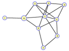
(a) Random

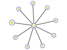
(b) Star

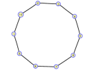
(c) Cycle

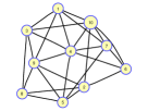
(d) k-NNG

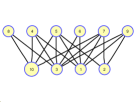
(e) Bipartite

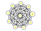
(f) Complete

Figure 1: Structures of the connected graph used in our numerical tests.

Strong Convexity

In the convex setting, for a fixed iteration number $T$, as the data size $mn$ increases and $\lambda$ decreases, $\epsilon_{\textrm{stab}}$ gets smaller for both diminishing and constant learning rates. However, similar to SGD, D-SGD also fails to have $\epsilon_{\textrm{stab}}$ under control when $T$ increases. This drawback does not exist in the strongly convex setting.

Strongly convex loss functions appear in the $\ell_{2}$ regularized machine learning models. As mentioned in Section 2, to guarantee the bounded gradient, the set $V$ should be restricted to a closed ball. We formulate the uniform stability results in this case in Theorem 2.

Theorem 2

Let $f(\cdot;\xi)$ be $\nu$-strongly convex and Assumptions 1, 2, 3 hold. If the step size $\alpha_{t}\equiv\alpha\leq{1}/{L}$, then D-SGD satisfies the uniform stability with

$$\epsilon_{\emph{stab}}\leq\frac{2B^{2}}{mn\nu}+\frac{4(1+\alpha B)B^{2}}{\nu}\frac{1_{\lambda\neq 0}}{1-\lambda}.$$

Furthermore, if the step size $\alpha_{t}=\frac{1}{\nu(t+1)}$, it holds that

$$\epsilon_{\emph{stab}}\leq\frac{2B^{2}}{mn\nu}+4(1+\frac{B}{\nu})\frac{B^{2}}{\nu}\frac{1_{\lambda\neq 0}}{1-\lambda}.$$

The uniformly stability bound for SGD with strong convexity is ${2B^{2}}/{(mn\nu)}$ (Hardt, Recht, and Singer 2016), which is smaller than the one of D-SGD. From Theorem 2, we see that the uniform stability bound of D-SGD is independent on the iterative number $T$. Moreover, D-SGD enjoys a smaller uniformly stable bound when the data size $mn$ is larger and $\lambda$ is smaller.

Nonconvexity

We now present the stability result for nonconvex loss functions.

Theorem 3

Suppose Assumptions 1, 2, 3 hold and $\sup_{{\bf x}\in V,\xi}f({\bf x};\xi)\leq 1$. For any $T$, if the step size $\alpha_{t}\leq{c}/{(t+1)}$ and $c$ is small enough, then D-SGD satisfies the uniform stability with

$$\epsilon_{\emph{stab}} \leq\frac{c^{\frac{1}{1+cL}}T^{\frac{cL}{1+cL}}}{mn}$$

$$+c^{\frac{1}{1+cL}}\Big{[}\frac{2B^{2}cL}{mn}+4(1+cB)B^{2}LC_{\lambda}\Big{]}T^{\frac{cL}{1+cL}}.$$

Without the convexity assumption, the uniform stable bound of D-SGD deteriorated. Theorem 3 shows that $\epsilon_{\textrm{stab}}=\mathcal{O}((1+C_{\lambda}){T^{\frac{cL}{1+cL}}}/{(mn)})$, which is much larger than the bounds in the convex case $\left(\mathcal{O}({\ln T}/{(mn)}+C_{\lambda}\ln T)\right)$.

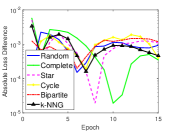
(a) Linear regression

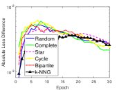
(b) Regularized logistic regression

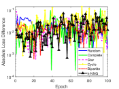
(c) ResNet-20 classification on Cifar-10

Figure 2: Comparison of the absolute loss difference under different graphs. (a), (b) and (c) correspond to the general convex, strongly convex, and nonconvex cases, respectively. In the strongly convex case, the curves become stable after enough iterations for all graphs. In the general convex case, the absolute loss difference oscillates and inferior to the strongly convex case. D-SGD performs worst in the nonconvex tests in terms of stability.

Excess Generalization for Convex Problems

In the nonconvex case, the optimization error of the function value is unclear. Thus, the excess generalization error is absent. We are also interested in the excess generalization associated with the computational optimization error. The existing computational errors of Algorithm 1 require extra assumptions on the graph for projections. However, these assumptions may fail to hold in many applications. Thus, we first present the optimization error of D-SGD when $f({\bf x};\xi)$ is convex without extra assumptions.

Optimization Error of Convex D-SGD

This part consists of optimization errors of D-SGD for convex and strongly convex settings. Assume ${\bf x}^{*}$ is the minimizer of $f({\bf x})$ over the set $V$, i.e., $f({\bf x}^{*})=\min_{{\bf x}\in V}f({\bf x})$.

Lemma 3

Let $f(\cdot;\xi)$ be convex and Assumptions 1, 2 hold, and let $({\bf x}^{t})_{1\leq t\leq T}$ be the sequence generated by D-SGD. Then

$$\mathbb{E}(f(\emph{ave}({\bf x}^{T}))-f({\bf x}^{*}))\leq\frac{\|{\bf x}^{1}-{\bf x}^{*}\|^{2}}{\sum_{t=1}^{T-1}\alpha_{t}}+\frac{2B^{2}\sum_{t=1}^{T-1}\alpha_{t}^{2}}{m\sum_{t=1}^{T-1}\alpha_{t}}$$

$$+8LrBM(T)+2\lambda^{2}B^{2}M(T)^{2},$$

where $M(T):=\max_{1\leq t\leq T-1}\{\sum_{j=0}^{t-1}\alpha_{j}\lambda^{t-1-j}\}$ and $r$ is the radius of $V$.

It is worth mentioning that the optimization error is established on the average point $\textrm{ave}({\bf x}^{T})$ for technical reasons.

In the following, we provide the results for the strongly convex setting.

Lemma 4

Let $f(\cdot;\xi)$ be $\nu$-strongly convex and Assumptions 1, 2, 3 hold, and let $V$ be a closed ball with radius $r>0$, and let $({\bf x}^{t})_{1\leq t\leq T}$ be the sequence generated by D-SGD. When $\alpha_{t}\equiv\alpha>0$, then

$$\mathbb{E}\|{\bf x}^{T}-{\bf x}^{*}\|^{2}\leq(1-2\alpha\nu)^{T-1}\|{\bf x}^{1}-{\bf x}^{*}\|^{2}$$

$$+(\frac{4\alpha LrB}{(1-\lambda)\nu}+\frac{\lambda^{2}B^{2}\alpha}{m(1-\lambda)^{2}\nu})1_{\lambda\neq 0},$$

where $1_{\lambda\neq 0}=1$ when $\lambda\neq 0$, and $1_{\lambda\neq 0}=0$ when $\lambda=0$. When $\alpha_{t}={1}/{(2\nu(t+1))}$, it then follows

$$\mathbb{E}\|{\bf x}^{T}-{\bf x}^{*}\|^{2}\leq\frac{\|{\bf x}^{1}-{\bf x}^{*}\|^{2}}{T-1}+\frac{D_{\lambda}\ln T}{T-1},$$

where $D_{\lambda}:=\frac{B^{2}}{2\nu^{2}}+\frac{\lambda^{2}B^{2}C_{\lambda}^{2}}{2\nu^{2}m}+\frac{2LrBC_{\lambda}}{\nu^{2}}$ and

$$C_{\lambda}:=\left\{\begin{array}[]{c}\ln\frac{1}{\lambda}\frac{\lambda^{\ln\frac{1}{\lambda}}}{\lambda}+\frac{\ln^{2}\frac{1}{\lambda}}{16\lambda}\lambda^{\frac{\ln\frac{1}{\lambda}}{8}}+\frac{2}{\lambda\ln\frac{1}{\lambda}}~{}~{}\lambda\neq 0,\\ 0,~{}~{}\lambda=0.\\ \end{array}\right.$$

The result shows that D-SGD with projection converges sublinearly in the strongly convex case. To reach an $\epsilon>0$ error, we shall set the iteration number as $\widetilde{\mathcal{O}}({1}/{\epsilon})$. Our result coincides with the existing convergence results of SGD with strong convexity (Rakhlin, Shamir, and Sridharan 2012). What is different is that D-SGD is affected by the parameter $\lambda$, which is determined by the structure of the connected graph.

General Convexity

Notice that the computational error of D-SGD, in this case, is described by $\textrm{ave}({\bf x}^{T})$. Thus, we need to estimate the generalization bound about $\textrm{ave}({\bf x}^{T})$.

Theorem 4

Let $f(\cdot;\xi)$ be convex and Assumptions 1, 2, 3 hold. If the step size $\alpha_{t}\equiv\alpha\leq{2}/{L}$, then the average output (5) obeys the following generalization bound

$$\epsilon_{\emph{ex-gen}}\leq\frac{2B^{2}\alpha(t-1)}{mn}+\frac{4\alpha B^{2}(1+\alpha B)(t-1)}{1-\lambda}1_{\lambda\neq 1}$$

$$+\frac{4r^{2}}{(T-1)\alpha}+\frac{2B^{2}\alpha}{m}+\frac{8LrB\alpha}{1-\lambda}1_{\lambda\neq 1}+\frac{2\lambda^{2}B^{2}\alpha^{2}}{(1-\lambda)^{2}}.$$

Furthermore, if the step size is chosen as $\alpha_{t}={1}/{(t+1)}$, we have

$$\epsilon_{\emph{ex-gen}}\leq\frac{B^{2}\ln T}{mn}+\frac{4B^{2}(1+B)}{\ln(T+1)}1_{\lambda\neq 1}+2\lambda^{2}B^{2}C_{\lambda}^{2}$$

$$+\frac{4r^{2}}{\ln(T+1)}+\frac{4B^{2}}{m\ln(T+1)}+8LrBC_{\lambda}1_{\lambda\neq 1}.$$

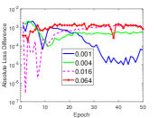
(a) Random

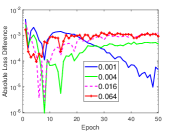
(b) Star

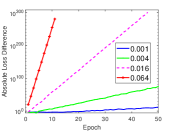
(c) Cycle

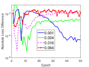
(d) k-NNG

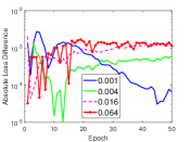
(e) Bipartite

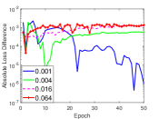
(f) Complete

Figure 3: Absolute loss difference versus epochs for linear regression task on Body Fat dataset. With current learning rates, D-SGD diverges for the Cycle graph. With enough iterations, the smaller learning rate can achieves a smaller difference for all graph.

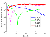
(a) Random

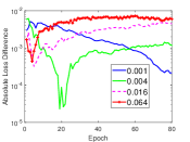
(b) Star

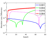
(c) Cycle

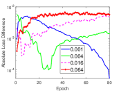
(d) k-NNG

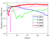
(e) Bipartite

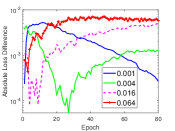
(f) Complete

Figure 4: Absolute loss difference versus epochs for the $\ell_{2}$ regularized logistic regression task on ijcnn1. The strongly convex tests are similar to general convex ones but more smooth. With strong convexity, D-SGD converges over the Cycle graph. In particular, when a smaller learning rate is used.

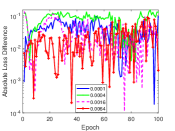
(a) Random

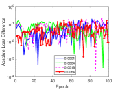
(b) Star

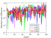
(c) Cycle

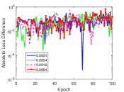
(d) k-NNG

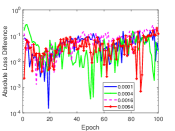
(e) Bipartite

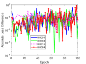
(f) Complete

Figure 5: Absolute loss difference versus epochs for training nonconvex machine learning model, i.e., ResNet20. Unlike the convex cases, the absolute loss difference oscillates chaotically, which implies worse stability.

Strong Convexity

Now, we present the excess generalization of D-SGD under strong convexity.

Theorem 5

Let $f(\cdot;\xi)$ be $\nu$-strongly convex and Assumptions 1, 2, 3 hold. If the step size $\alpha_{t}\equiv\alpha\leq{1}/{L}$, the excess generalization bound is

$$\epsilon_{\emph{ex-gen}}\leq\frac{2B^{2}}{mn\nu}+\frac{4(1+\alpha B)B^{2}}{\nu}\frac{1_{\lambda\neq 0}}{1-\lambda}$$

$$+B\sqrt{(1-2\alpha\nu)^{T-1}4r^{2}+(\frac{4\alpha LrB}{(1-\lambda)\nu}+\frac{\lambda^{2}B^{2}\alpha}{m(1-\lambda)^{2}\nu})1_{\lambda\neq 0}}.$$

Furthermore, if the step size $\alpha_{t}={1}/{(\nu(t+1))}$, the excess generalization bound is

$$\epsilon_{\emph{ex-gen}} \leq\frac{2B^{2}}{mn\nu}+\frac{4(\nu+B)B^{2}}{\nu^{2}}\frac{1_{\lambda\neq 0}}{1-\lambda}+B\sqrt{\frac{4r^{2}}{T-1}+\frac{D_{\lambda}\ln T}{T-1}}.$$

Numerical Results

We numerically verify our theoretical findings in this section, with a focus on testing three kinds of models, namely, strongly convex, convex, and nonconvex. For all the above three scenarios, we set the number of nodes $m$ to 10 and conduct two kinds of experiments: the first kind of experiments is to verify the stability and generalization results. Given a fixed graph, we use two sets of samples that are of the same amount, and the entries are differing by a small portion. We compare the training loss and training accuracy of D-SGD on these two datasets; the second kind is to demonstrate the effects due to the structure of the connected graph. We run our experiments on different types of connected graphs with the same dataset. In particular, we test six different connected graphs, as shown in Figure 1.

Convex case

We consider the following optimization problem

$$\min_{{\bf x}\in\mathbb{R}^{14}}\Phi({\bf x}):=\frac{1}{504}\sum_{i=1}^{252}\|\xi_{i}^{\top}{\bf x}-{\bf y}_{i}\|^{2},$$

which arises from a simple regression problem. Here, we use the Body Fat dataset (Johnson 1996) which contains 252 samples. We run D-SGD on two subsets of the Body Fat dataset, and both of size 200. Let ${\bf x}^{k}$ and $\widehat{{\bf x}}^{k}$ be the outputs of the D-SGD on the two different subsets. We define the absolute loss difference as $|\Phi({\bf x}^{k})-\Phi(\widehat{{\bf x}}^{k})|.$ For the above six graphs, we record the absolute difference in the value of function $\Phi$ for a set of learning rate, namely, $\{0.001,0.004,0.016,0.064\}$ in Figure 3. In the second test, we use the learning rate $0.001$ and compare the absolute loss difference with different graphs in Figure 2 (a). Our results show that the smaller learning rate usually yields a smaller loss difference, and the complete graph can achieve the smallest bound. These observations are consistent with our theoretical results for the convex D-SGD.

Strongly convex case

To verify our theory on the strongly convex case, we consider the regularized logistic regression model as follows

$$\min_{{\bf x}\in\mathbb{R}^{22}}\left\{\frac{1}{9000}\sum_{i=1}^{9000}\left(\log(1+\textrm{exp}(-b_{i}{\bf a}^{\top}_{i}{\bf x}))+\frac{\lambda}{2}\|{\bf x}\|^{2}\right)\right\}.$$

We use the benchmark ijcnn1 dataset(Rennie and Rifkin 2001) and set $\lambda=10^{-4}$. Two 8000-sample sub-datasets with 1000 different samples are used as the test set. We conduct experiments on the two datasets with the same set of learning rates that are used in the last subsection. The absolute loss difference under different learning rates is plotted in Figure 4, and the performance under different graphs is reported in Figure 2 (b). The results of D-SGD in the strongly convex case is similar to the convex case. Also, note that the absolute loss difference increases as the learning rates grow.

Nonconvex case

We test ResNet-20 (He et al. 2016) for CIFAR10 classification (Krizhevsky 2009). We adopt two different 40000-sample subsets. The loss values are built on the test set. The absolute loss difference with the learning rate set $\{0.0001,0.0004,0.0016,0.0064\}$ versus the epochs is presented in Figure 5, and the absolute loss difference with different graphs are shown in Figure 5 (c). 100 epochs are used in the nonconvex test. The results show that the nonconvex D-SGD is much more unstable than the convex ones, which matches our theoretical findings.

Conclusion

In this paper, we develop the stability and generalization error for the (projected) decentralized stochastic gradient descent (D-SGD) in strongly convex, convex, and nonconvex settings. In contrast to the previous works on the analysis of the projected decentralized gradient descent, our theories are built on much more relaxed assumptions. Our theoretical results show that the stability and generalization of D-SGD depend on the learning rate and the structure of the connected graph. Furthermore, we prove that decentralization deteriorates the stability of D-SGD. Our theoretical results are empirically supported by experiments on training different machine learning models in different decentralization settings. There are numerous avenues for future work: 1) deriving the improved stability and generalization bounds of D-SGD in the general convex and nonconvex cases, 2) proving the high probability bounds, 3) studying the stability and generalization bound of the moment variance of D-SGD.

Supplementary materials for

Stability and Generalization Bounds of Decentralized Stochastic Gradient Descent

Appendix A More results of the test

We present the absolute accuracy difference in the decentralized neutral networks training.

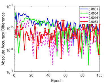
(a) Random

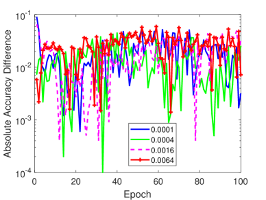
(b) Star

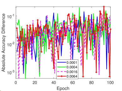
(c) Cycle

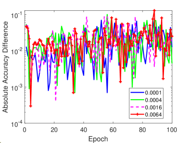
(d) k-NNG

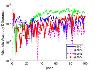
(e) Bipartite

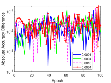
(f) Complete

Figure 6: Absolute accuracy difference versus epochs for nonconvex model. The absolute accuracy difference performs similarly to the absolute loss difference.

Appendix B Technical Lemmas

Lemma 5

For any $0<\lambda<1$ and $t\in\mathbb{Z}^{+}$, it holds

$$\sum_{j=0}^{t-1}\frac{\lambda^{t-1-j}}{j+1}\leq\frac{C_{\lambda}}{t}$$

with $C_{\lambda}:=\ln\frac{1}{\lambda}\frac{\lambda^{\ln\frac{1}{\lambda}}}{\lambda}+\frac{\ln^{2}\frac{1}{\lambda}}{16\lambda}\lambda^{\frac{\ln\frac{1}{\lambda}}{8}}+\frac{2}{\lambda\ln\frac{1}{\lambda}}$.

Lemma 6

[Lemmas 2.5 and 3.7, (Hardt, Recht, and Singer 2016)] Fix an arbitrary sequence of updates $G_{1},\dots,G_{T}$ and another sequence $G_{1}^{\prime},\dots,G_{T}^{\prime}.$ Let ${\bf x}^{0}={\bf y}^{0}$ be a starting point in $V$ and define $\delta_{t}=\|{\bf x}^{t}-{\bf y}^{t}\|$ where ${\bf x}^{t},{\bf y}^{t}$ are defined recursively through

$${\bf x}^{t+1}=G_{t}({\bf x}^{t}),\,\,~{}~{}\,~{}~{}{\bf y}^{t+1}=G_{t}^{\prime}({\bf y}^{t}).$$

Then, we have the recurrence relation $\delta_{0}=0$,

$$\delta_{t+1} \leq\begin{cases}\eta\delta_{t}&\text{$G_{t}=G_{t}^{\prime}$ is $\eta$-expansive}\\ \min(\eta,1)\delta_{t}+2\sigma_{t}&\text{$G_{t}$ and $G_{t}^{\prime}$ are $\sigma$-bounded,}\,\text{$G_{t}$ is $\eta$ expansive.}\end{cases}$$

For a nonnegative step size $\alpha\geq 0$ and a function $f\colon V\to\mathbb{R},$ we define $G_{f,\alpha}$ as

$$G_{f,\alpha}({\bf x})=\textbf{\emph{Proj}}_{V}({\bf x}-\alpha\nabla f({\bf x})),$$

where $V$ is a closed convex set. Assume that $f$ is $L$-smooth. Then, the following properties hold.

• $G_{f,\alpha}$ is $(1+\alpha L)$-expansive.

• If $f$ is convex. Then, for any $\alpha\leq 2/L,$ the gradient update $G_{f,\alpha}$ is $1$-expansive.

• If $f$ is $\nu$-strongly convex. Then, for $\alpha\leq\frac{1}{L}$, $G_{f,\alpha}$ is $\left(1-\alpha\nu\right)$-expansive.

Lemma 7

Let Assumption 1 hold. Assume two sample sets $S$ and $S^{\prime}$ just differs at one sample in the first $n$ sample. And let ${\bf x}^{T}$ and ${\bf y}^{T}$ be the corresponding outputs of D-SGD applied to these two sets after $T$ steps. Then, for every $\xi\sim\mathcal{D}$ and every $t_{0}\in\{0,1,\dots,n\},$ under both the random update rule and the random permutation rule, we have

$$\mathbb{E}\left|f({\bf x}^{T};\xi)-f({\bf y}^{T};\xi)\right|\leq\frac{t_{0}}{n}\sup_{{\bf x}\in V,\xi}f({\bf x};\xi)+B\mathbb{E}\left[\delta_{T}\mid\delta_{t_{0}}=0\right].$$

Lemma 8

Given the stepsize $(\alpha_{t})_{t\geq 0}>0$ and assume $({\bf x}^{t}(i))_{t\geq 0}$ are generated by D-SGD for all $i\in\{1,2\ldots,m\}$. If Assumption 3 holds, we have the following bound

$$\left[\sum_{i=1}^{m}\|{\bf x}^{t}(i)-{\bf x}^{t}\|^{2}\right]^{\frac{1}{2}}\leq 2\sqrt{m}B\sum_{j=0}^{t-1}\alpha_{j}\lambda^{t-1-j}.$$ (6)

Lemma 9

Denote the matrix ${\bf X}^{t}:=\begin{bmatrix}{\bf x}^{t}(1),{\bf x}^{t}(2),\ldots,{\bf x}^{t}(m)\end{bmatrix}^{\top}\in\mathbb{R}^{m\times d}$. Assume the conditions of Lemma 8 hold, we then get

$$\|({\bf W}-{\bf P}){\bf X}^{t}\|\leq\sqrt{m}B\sum_{j=0}^{t-1}\alpha_{j}\lambda^{t-j}.$$ (7)

Appendix C Proofs of Technical Lemmas

Proof of Lemma 5

For any $x\in[j,j+1]$, $j+1\geq x$ and $\lambda^{t-1-j}\leq\lambda^{t-1-x}$, we then get

$$\sum_{j=0}^{t-1}\frac{\lambda^{t-1-j}}{j+1}=\lambda^{t-1}+\sum_{j=1}^{t-1}\frac{\lambda^{t-1-j}}{j+1}\leq\lambda^{t-1}+\sum_{j=1}^{t-1}\int_{j}^{j+1}\frac{\lambda^{t-1-x}}{x}dx$$ (8)

$$=\lambda^{t-1}+\lambda^{t-1}\int_{1}^{t}\frac{\lambda^{-x}}{x}dx.$$

We turn to the bound

$$\begin{aligned} &\int_{1}^{t}\frac{\lambda^{-x}}{x}dx=\int_{1}^{\frac{t}{2}}\frac{\lambda^{-x}}{x}dx+\int_{\frac{t}{2}}^{t}\frac{\lambda^{-x}}{x}dx\\ &\leq\lambda^{-\frac{t}{2}}\int_{1}^{\frac{t}{2}}\frac{1}{x}dx+\frac{2}{t}\int_{\frac{t}{2}}^{t}\lambda^{-x}dx\leq\lambda^{-\frac{t}{2}}\ln t+\frac{2\lambda^{-t}}{t\ln\frac{1}{\lambda}}\end{aligned}.$$

With (8), we are then led to

$$\sum_{j=0}^{t-1}\frac{\lambda^{t-1-j}}{j+1}\leq\lambda^{t-1}+\lambda^{\frac{t}{2}-1}t+\frac{2}{t\lambda\ln\frac{1}{\lambda}},$$

where we used the fact $\ln t\leq t$. Now, we provide the bounds for $\sup_{t\geq 1}\{t\lambda^{t-1}+\lambda^{\frac{t}{2}-1}t^{2}\}\leq\sup_{t\geq 1}\{t\lambda^{t-1}\}+\sup_{t\geq 1}\{\lambda^{\frac{t}{2}-1}t^{2}\}$. Note that $\ln(t\lambda^{t-1})=\ln t+(t-1)\ln\lambda$, whose derivative is $\frac{1}{t}+\ln\lambda$. It is easy to check that $t=\ln\frac{1}{\lambda}$ achieves the maximum, which indicates

$$\sup_{t\geq 1}\{t\lambda^{t-1}\}\leq\ln\frac{1}{\lambda}\frac{\lambda^{\ln\frac{1}{\lambda}}}{\lambda}.$$

Similarly, we get

$$\sup_{t\geq 1}\{\lambda^{\frac{t}{2}-1}t^{2}\}\leq\frac{\ln^{2}\frac{1}{\lambda}}{16\lambda}\lambda^{\frac{\ln\frac{1}{\lambda}}{8}}.$$

Proof of Lemma 7

Proof of Lemma 7 is almost identical to the proof of Lemma 3.11 in (Hardt, Recht, and Singer 2016).

Proof of Lemma 8

We denote that

$${\bf\zeta}^{t}:=\alpha_{t}\begin{bmatrix}\nabla f({\bf x}^{t}(1);\xi_{j_{t}(1)}),\nabla f({\bf x}^{t}(2);\xi_{j_{t}(2)}),\ldots,\nabla f({\bf x}^{t}(m);\xi_{j_{t}(m)})\end{bmatrix}^{\top}\in\mathbb{R}^{m\times d}.$$

With Assumption 1, $\|{\bf\zeta}^{t}\|\leq\alpha_{t}\sqrt{m}B$. Then the global scheme can be presented as

$${\bf X}^{t+1}=\textbf{Proj}_{V^{m}}\Big{[}{\bf W}{\bf X}^{t}-{\bf\zeta}^{t}\Big{]},$$ (9)

where $V^{m}:=\underbrace{V\oplus V\ldots\oplus V}_{m}$. Noticing the fact

$${\bf W}{\bf P}={\bf P}{\bf W}={\bf P}.$$ (10)

With Lemma 2, we have

$$\|{\bf W}-{\bf P}\|_{\textrm{op}}\leq\lambda.$$

Multiplication of both sides of (9) with ${\bf P}$ together with (10) then tells us

$$(\mathbb{I}-{\bf P}){\bf X}^{t+1}=(\mathbb{I}-{\bf P})\textbf{Proj}_{V^{m}}\Big{[}{\bf W}{\bf X}^{t}-{\bf\zeta}^{t}\Big{]}$$ (11)

$$=\textbf{Proj}_{V^{m}}\Big{[}{\bf W}{\bf X}^{t}-{\bf\zeta}^{t}\Big{]}-{\bf P}\cdot\textbf{Proj}_{V^{m}}\Big{[}{\bf W}{\bf X}^{t}\Big{]}+{\bf P}\cdot\textbf{Proj}_{V^{m}}\Big{[}{\bf W}{\bf X}^{t}\Big{]}-{\bf P}\cdot\textbf{Proj}_{V^{m}}\Big{[}{\bf W}{\bf X}^{t}-{\bf\zeta}^{t}\Big{]}.$$

It is easy to check that ${\bf W}{\bf X}^{t}\in V^{m}$ and ${\bf P}{\bf W}{\bf X}^{t}\in V^{m}$. Thus, it follows ${\bf P}\cdot\textbf{Proj}_{V^{m}}\Big{[}{\bf W}{\bf X}^{t}\Big{]}={\bf P}{\bf W}{\bf X}^{t}=\textbf{Proj}_{V^{m}}\Big{[}{\bf P}{\bf W}{\bf X}^{t}\Big{]}$. From (11), letting $\mathbb{I}\in\mathbb{R}^{m}$ be the identical matrix,

$$\|(\mathbb{I}-{\bf P}){\bf X}^{t+1}\|\leq\left\|\textbf{Proj}_{V^{m}}\Big{[}{\bf W}{\bf X}^{t}-{\bf\zeta}^{t}\Big{]}-\textbf{Proj}_{V^{m}}\Big{[}{\bf P}{\bf W}{\bf X}^{t}\Big{]}\right\|+\|{\bf\zeta}^{t}\|$$ (12)

$$\qquad\leq\|{\bf W}{\bf X}^{t}-{\bf\zeta}^{t}-{\bf P}{\bf W}{\bf X}^{t}\|+\sqrt{m}B\alpha_{t}\leq\|{\bf W}{\bf X}^{t}-{\bf P}{\bf W}{\bf X}^{t}\|+2\sqrt{m}B\alpha_{t}$$

$$\qquad\overset{a)}{\leq}\|({\bf W}-{\bf P})(\mathbb{I}-{\bf P}){\bf X}^{t}\|+2\sqrt{m}B\alpha_{t}\overset{b)}{\leq}\lambda\|(\mathbb{I}-{\bf P}){\bf X}^{t}\|+2\sqrt{m}B\alpha_{t}.$$

where $a)$ uses the fact $({\bf W}-{\bf P})(\mathbb{I}-{\bf P})={\bf W}-2{\bf P}+{\bf W}{\bf P}={\bf W}-{\bf P}={\bf W}-{\bf P}W$, and $b)$ depends on Lemma 2. Then, we derive

$$\|{\bf X}^{t}-{\bf P}{\bf X}^{t}\|\leq 2\sqrt{m}B\sum_{j=0}^{t-1}\alpha_{j}\lambda^{t-1-j}.$$ (13)

where we used initialization ${\bf X}^{0}=\textbf{0}$.

Proof of Lemma 9

Direct computations give

$$({\bf W}-{\bf P}){\bf X}^{t+1} =({\bf W}-{\bf P}){\bf W}{\bf X}^{t}-({\bf W}-{\bf P}){\bf\zeta}^{t}$$

$$=({\bf W}-{\bf P})({\bf W}-{\bf P}){\bf X}^{t}-({\bf W}-{\bf P}){\bf\zeta}^{t},$$

where we used $(W-{\bf P})W=(W-{\bf P})(W-{\bf P})$. Thus, we obtain

$$\|(W-{\bf P}){\bf X}^{t+1}\|\leq\lambda\|(W-{\bf P}){\bf X}^{t}\|+\sqrt{m}\lambda B\alpha_{t},$$

Appendix D Proof of Theorem 1

Without loss of generalization , assume two sample sets $S$ and $S^{\prime}$ just differs at one sample in the first $m$ sample. And let ${\bf x}^{t}$ and ${\bf y}^{t}$ be the corresponding outputs of D-SGD applied to these two sets. Denoting that

$$\delta_{t}:=\|{\bf x}^{t}-{\bf y}^{t}\|.$$

At iteration $t$, with probability $1-\frac{1}{n}$,

$${\bf x}^{t+1}-{\bf y}^{t+1} =\frac{\sum_{i=1}^{m}\left[\textbf{Proj}_{V}[\sum_{l\in\mathcal{N}(i)}w_{i,l}{\bf x}^{t}(l)-\alpha_{t}\nabla f({\bf x}^{t}(i);\xi_{j_{t}(i)})]-\textbf{Proj}_{V}[\sum_{l\in\mathcal{N}(i)}w_{i,l}{\bf y}^{t}(l)-\alpha_{t}\nabla f({\bf y}^{t}(i);\xi_{j_{t}(i)})]\right]}{m}$$ (14)

$$=\underbrace{\frac{\sum_{i=1}^{m}\left[\textbf{Proj}_{V}[{\bf x}^{t}-\alpha_{t}\nabla f({\bf x}^{t};\xi_{j_{t}(i)})]-\textbf{Proj}_{V}[{\bf y}^{t}-\alpha_{t}\nabla f({\bf y}^{t};\xi_{j_{t}(i)})]\right]}{m}}_{\S}+\wp_{t}.$$

With gradient smooth assumption,

$$\|\wp_{t}\| \leq\frac{\sum_{i=1}^{m}(\sum_{l\in\mathcal{N}(i)}w_{i,l}\|{\bf x}^{t}(l)-{\bf x}^{t}\|+\alpha_{t}B\|{\bf x}^{t}(i)-{\bf x}^{t}\|)}{m}+\frac{\sum_{i=1}^{m}(\sum_{l\in\mathcal{N}(i)}w_{i,l}\|{\bf y}^{t}(l)-{\bf y}^{t}\|+\alpha_{t}B\|{\bf y}^{t}(i)-{\bf y}^{t}\|)}{m}$$ (15)

$$\leq\frac{\sum_{i=1}^{m}(\sum_{l=1}^{m}w_{i,l}\|{\bf x}^{t}(l)-{\bf x}^{t}\|+\alpha_{t}B\|{\bf x}^{t}(i)-{\bf x}^{t}\|)}{m}+\frac{\sum_{i=1}^{m}(\sum_{l=1}^{m}w_{i,l}\|{\bf y}^{t}(l)-{\bf y}^{t}\|+\alpha_{t}B\|{\bf y}^{t}(i)-{\bf y}^{t}\|)}{m}$$

$$\leq\frac{\sum_{l=1}^{m}\|{\bf x}^{t}(l)-{\bf x}^{t}\|+\alpha_{t}B\sum_{i=1}^{m}\|{\bf x}^{t}(i)-{\bf x}^{t}\|}{m}+\frac{\sum_{l=1}^{m}\|{\bf y}^{t}(l)-{\bf y}^{t}\|+\alpha_{t}B\sum_{i=1}^{m}\|{\bf y}^{t}(i)-{\bf y}^{t}\|}{m}$$

$$\leq\frac{(1+\alpha_{t}B)\sqrt{m}[\sum_{i=1}^{m}\|{\bf x}^{t}(i)-{\bf x}^{t}\|^{2}]^{\frac{1}{2}}}{m}+\frac{(1+\alpha_{t}B)\sqrt{m}[\sum_{i=1}^{m}\|{\bf y}^{t}(i)-{\bf y}^{t}\|^{2}]^{\frac{1}{2}}}{m}$$

$$\leq 4(1+\alpha_{t}B)B\sum_{j=0}^{t-1}\alpha_{j}\lambda^{t-1-j}.$$

Due to the convexity, $\textbf{Proj}_{V}[\cdot-\alpha_{t}\nabla f(\cdot;\xi_{j_{t}(i)})]$ is 1-expansive when $\alpha_{t}\leq\frac{2}{L}$. Thus, we have

$$\|\S\|\leq\|{\bf x}^{t}-{\bf y}^{t}\|=\delta_{t}.$$

With probability $\frac{1}{n}$,

$${\bf x}^{t+1}-{\bf y}^{t+1} =\frac{\sum_{i=2}^{m}\left[\textbf{Proj}_{V}[\sum_{l\in\mathcal{N}(i)}w_{i,l}{\bf x}^{t}(l)-\alpha_{t}\nabla f({\bf x}^{t};\xi_{j_{t}(i)})]-\textbf{Proj}_{V}[\sum_{l\in\mathcal{N}(i)}w_{i,l}{\bf y}^{t}(l)-\alpha_{t}\nabla f({\bf y}^{t};\xi_{j_{t}(i)})]\right]}{m}$$ (16)

$$+\frac{\left[\textbf{Proj}_{V}[\sum_{l\in\mathcal{N}(1)}w_{1,l}{\bf x}^{t}(l)-\alpha_{t}\nabla f({\bf x}^{t};\xi^{\prime}_{j_{t}(1)})]-\textbf{Proj}_{V}[\sum_{l\in\mathcal{N}(1)}w_{1,l}{\bf y}^{t}(l)-\alpha_{t}\nabla f({\bf y}^{t};\xi_{j_{t}(1)})]\right]}{m}+\Im_{t}$$

$$=\underbrace{\frac{\sum_{i=2}^{m}\left[\textbf{Proj}_{V}[{\bf x}^{t}-\alpha_{t}\nabla f({\bf x}^{t};\xi_{j_{t}(i)})]-\textbf{Proj}_{V}[{\bf y}^{t}-\alpha_{t}\nabla f({\bf y}^{t};\xi_{j_{t}(i)})]\right]}{m}}_{\sharp}$$

$$+\frac{\left[\textbf{Proj}_{V}[{\bf x}^{t}-\alpha_{t}\nabla f({\bf x}^{t};\xi^{\prime}_{j_{t}(1)})]-\textbf{Proj}_{V}[{\bf y}^{t}-\alpha_{t}\nabla f({\bf y}^{t};\xi_{j_{t}(1)})]\right]}{m}+\Im_{t}.$$

It is easy to check that $\|\Im_{t}\|\leq 4(1+\alpha_{t}B)B\sum_{j=0}^{t-1}\alpha_{j}\lambda^{t-1-j}$. With Lemma 6, we have

$$\|\sharp\|\leq\frac{m-1}{m}\delta_{t},~{}\,~{}\,~{}\left\|\frac{\left[\textbf{Proj}_{V}[{\bf x}^{t}-\alpha_{t}\nabla f({\bf x}^{t};\xi_{j^{\prime}_{t}(1)})]-\textbf{Proj}_{V}[{\bf y}^{t}-\alpha_{t}\nabla f({\bf y}^{t};\xi_{j_{t}(1)})]\right]}{m}\right\|\leq\frac{\delta_{t}+2B\alpha_{t}}{m}.$$

Thus, we derive

$$\mathbb{E}\delta_{t+1}\leq\mathbb{E}\delta_{t}+\frac{2B\alpha_{t}}{mn}+4(1+\alpha_{t}B)B\sum_{j=0}^{t-1}\alpha_{j}\lambda^{t-1-j}.$$

That also means

$$\mathbb{E}\delta_{T}\leq\frac{2B\sum_{t=0}^{T-1}\alpha_{t}}{mn}+4B\sum_{t=0}^{T-1}(1+\alpha_{t}B)\sum_{j=0}^{t-1}\alpha_{j}\lambda^{t-1-j}.$$

Noticing the fact

$$\mathbb{E}|f({\bf x}^{T};\xi)-f({\bf y}^{T};\xi)|\leq B\mathbb{E}\|{\bf x}^{T}-{\bf y}^{T}\|=B\mathbb{E}\delta_{T},$$ (17)

we then proved the result.

Appendix E Proof of Proposition 1

Let ${\bf x}^{t}$ and ${\bf y}^{t}$ be the output of D-SGD with only one different sample after $t$ iterations. We have

$$\|\textrm{ave}({\bf x}^{T})-\textrm{ave}({\bf y}^{T})\|=\left\|\frac{\sum_{t=1}^{T-1}\alpha_{t}({\bf x}^{t}-{\bf y}^{t})}{\sum_{t=1}^{T-1}\alpha_{t}}\right\|\leq\frac{\sum_{t=1}^{T-1}\alpha_{t}\|{\bf x}^{t}-{\bf y}^{t}\|}{\sum_{t=1}^{T-1}\alpha_{t}}.$$

As the same proofs in Theorem 1, we can derive

$$\|{\bf x}^{t}-{\bf y}^{t}\|\leq\frac{2B\sum_{k=1}^{t-1}\alpha_{k}}{mn}+4B\sum_{k=1}^{t-1}(1+\alpha_{k}B)\sum_{j=0}^{k-1}\alpha_{j}\lambda^{k-1-j}.$$

1) when $\alpha_{t}\equiv\alpha$, we have

$$\|{\bf x}^{t}-{\bf y}^{t}\|\leq\frac{2B\alpha(t-1)}{mn}+\frac{4\alpha B(1+\alpha B)(t-1)}{1-\lambda}1_{\lambda\neq 1}.$$

Thus, we get

$$\|\textrm{ave}({\bf x}^{T})-\textrm{ave}({\bf y}^{T})\|\leq\frac{B\alpha(t-1)}{mn}+\frac{2\alpha B(1+\alpha B)(t-1)}{1-\lambda}1_{\lambda\neq 1}.$$

2) when $\alpha_{t}=\frac{1}{t+1}$, we have

$$\|{\bf x}^{t}-{\bf y}^{t}\|\leq\frac{2B\ln t}{mn}+\frac{4\alpha B(1+B)C_{\lambda}}{t}1_{\lambda\neq 1}.$$

Thus, we get

$$\|\textrm{ave}({\bf x}^{T})-\textrm{ave}({\bf y}^{T})\|\leq\frac{B\ln T}{mn}+\frac{4\alpha B(1+B)}{\ln(T+1)}1_{\lambda\neq 1}.$$

The Lipschitz continuity of the loss function then proves the result.

Appendix F Proof of Theorem 2

Without loss of generalization , we assume $\lambda\neq 0$. Due to the strong convexity with $\nu$, $\textbf{Proj}_{V}[\cdot-\alpha_{t}\nabla f(\cdot;\xi_{j_{t}(i)})]$ is $(1-\alpha_{t}\nu)$-contractive when $\alpha_{t}\leq\frac{1}{L}$. Thus, in (14), it holds

$$\|\S\|\leq(1-\alpha_{t}\nu)\|{\bf x}^{t}-\overline{{\bf x}}^{t}\|=(1-\alpha_{t}\nu)\delta_{t};$$

and in (16),

$$\|\sharp\|\leq\frac{m-1}{m}(1-\alpha_{t}\nu)\delta_{t},$$

$$\left\|\frac{\left[\textbf{Proj}_{V}[{\bf x}^{t}-\alpha_{t}\nabla f({\bf x}^{t};\xi_{j^{\prime}_{t}(1)})]-\textbf{Proj}_{V}[{\bf y}^{t}-\alpha_{t}\nabla f({\bf y}^{t};\xi_{j_{t}(1)})]\right]}{m}\right\|\leq\frac{(1-\alpha_{t}\nu)\delta_{t}+2B\alpha_{t}}{m}.$$

Therefore, we can get

$$\mathbb{E}\delta_{t+1}\leq(1-\alpha_{t}\nu)\mathbb{E}\delta_{t}+\frac{2B\alpha_{t}}{mn}+4(1+\alpha_{t}B)B\sum_{j=0}^{t-1}\lambda^{t-1-j}\alpha_{j}.$$ (18)

a) When $0<\lambda<1$, $\sum_{j=0}^{t-1}\lambda^{t-1-j}\leq\frac{1}{1-\lambda}$ and $\alpha_{t}\equiv\alpha$. Then we are led to

$$\mathbb{E}\delta_{t+1}\leq(1-\alpha\nu)\mathbb{E}\delta_{t}+\frac{2B\alpha}{mn}+4(1+\alpha B)B\alpha\frac{1}{1-\lambda}.$$

The recursion of inequality gives us

$$\mathbb{E}\delta_{T}\leq\sum_{t=0}^{T-1}(1-\alpha\nu)^{t}\left[\frac{2B\alpha}{mn}+4(1+\alpha B)B\alpha\frac{1}{1-\lambda}\right]=\frac{2B}{mn\nu}+\frac{4(1+\alpha B)B}{\nu}\frac{1}{1-\lambda}.$$

Once using (17), we then get the result.

b) In (18), by replacing $\alpha$ with $\alpha_{t}=\frac{1}{\nu(t+1)}$,

$$\mathbb{E}\delta_{t+1}\leq(1-\frac{1}{t+1})\mathbb{E}\delta_{t}+\Big{[}\frac{2B}{\nu mn}+4(1+\frac{B}{\nu})\frac{B}{\nu}\frac{1_{\lambda\neq 0}}{1-\lambda}\Big{]}\frac{1}{t+1}.$$ (19)

Thus, we get

$$\mathbb{E}\delta_{t}\leq\frac{2B}{\nu mn}+4(1+\frac{B}{\nu})\frac{B}{\nu}\frac{1_{\lambda\neq 0}}{1-\lambda}.$$ (20)

Appendix G Proof of Theorem 3

Assume $t_{0}\in\{1,2,\ldots,n\}$ to be determined, with Lemma 7,

$$\mathbb{E}\left|f({\bf x}^{T};\xi)-f({\bf y}^{T};\xi)\right|\leq\frac{t_{0}}{n}+L\mathbb{E}\left[\delta_{T}\mid\delta_{t_{0}}=0\right],$$

where we used $\sup_{{\bf x}\in V,\xi}f({\bf x};\xi)\leq 1$. In the following, we consider the case $\delta_{t_{0}}=0$. With Lemma 6, in (14),

$$\|\S\|\leq(1+\alpha_{t}L)\|{\bf x}^{t}-{\bf y}^{t}\|=(1+\alpha_{t}L)\delta_{t};$$

and in (16),

$$\|\sharp\|\leq\frac{m-1}{m}(1+\alpha_{t}L)\delta_{t},$$

$$~{}\left\|\frac{\left[\textbf{Proj}_{V}[{\bf x}^{t}-\alpha_{t}\nabla f({\bf x}^{t};\xi_{j^{\prime}_{t}(1)})]-\textbf{Proj}_{V}[{\bf y}^{t}-\alpha_{t}\nabla f({\bf y}^{t};\xi_{j_{t}(1)})]\right]}{m}\right\|\leq\frac{\delta_{t}+2B\alpha_{t}}{m}.$$

Therefore, when $t>t_{0}$, we can get

$$\mathbb{E}(\delta_{t+1}\mid\delta_{t_{0}}=0) \leq(1-\frac{1}{n})(1+\alpha_{t}L)\mathbb{E}(\delta_{t}\mid\delta_{t_{0}}=0)+\frac{1}{n}\Big{[}\frac{m-1}{m}(1+\alpha_{t}L)+\frac{1}{m}\Big{]}\delta_{t}$$

$$+\frac{2B\alpha_{t}}{mn}+4(1+\alpha_{t}B)B\sum_{j=0}^{t-1}\alpha_{j}\lambda^{t-1-j}$$

$$=\Big{[}1+(1-\frac{1}{mn})\alpha_{t}L\Big{]}\mathbb{E}(\delta_{t}\mid\delta_{t_{0}}=0)+\frac{2B\alpha_{t}}{mn}+4(1+\alpha_{t}B)B\sum_{j=0}^{t-1}\alpha_{j}\lambda^{t-1-j}.$$

With $\alpha\leq\frac{c}{t}$ and Lemma 5, we are then led to

$$\mathbb{E}(\delta_{t+1}\mid\delta_{t_{0}}=0) \leq\Big{[}1+cL(1-\frac{1}{mn})/t\Big{]}\mathbb{E}(\delta_{t}\mid\delta_{t_{0}}=0)+(\frac{2Bc}{mn}+4(1+cB)BC_{\lambda})/t$$

$$\leq\exp(cL(1-\frac{1}{mn})/t)\mathbb{E}(\delta_{t}\mid\delta_{t_{0}}=0)+(\frac{2Bc}{mn}+4(1+cB)BC_{\lambda})/t.$$

That then yields

$$\mathbb{E}(\delta_{T}\mid\delta_{t_{0}}=0) \leq\sum_{t=t_{0}+1}^{T}\Big{[}\exp(\sum_{i=t+1}^{T}cL(1-\frac{1}{mn})/i)\Big{]}(\frac{2Bc}{mn}+4(1+cB)BC_{\lambda})/t$$

$$\leq\sum_{t=t_{0}+1}^{T}\Big{[}\exp(cL(1-\frac{1}{mn})\ln\frac{T}{t})\Big{]}(\frac{2Bc}{mn}+4(1+cB)BC_{\lambda})/t$$

$$=(\frac{2Bc}{mn}+4(1+cB)BC_{\lambda})T^{cL(1-\frac{1}{mn})}\sum_{t=t_{0}+1}^{T}\frac{1}{t^{cL(1-\frac{1}{mn})+1}}$$

$$\leq(\frac{2Bc}{mn}+4(1+cB)BC_{\lambda})T^{cL(1-\frac{1}{mn})}\frac{cL(1-\frac{1}{mn})}{t_{0}^{cL(1-\frac{1}{mn})}}$$

$$\leq(\frac{2Bc}{mn}+4(1+cB)BC_{\lambda})cL\frac{T^{cL}}{t_{0}^{cL}}$$

From Lemma 7, we get

$$\mathbb{E}\left|f({\bf x}^{T};\xi)-f({\bf y}^{T};\xi)\right|\leq\frac{t_{0}}{mn}+BcL(\frac{2Bc}{mn}+4(1+cB)BC_{\lambda})\frac{T^{cL}}{t_{0}^{cL}}.$$

Setting $t_{0}=c^{\frac{1}{1+cL}}T^{\frac{cL}{1+cL}}$, when $c$ is small enough, $t_{0}\leq n$. We then have

$$\mathbb{E}\left|f({\bf x}^{T};\xi)-f({\bf y}^{T};\xi)\right|\leq\frac{c^{\frac{1}{1+cL}}T^{\frac{cL}{1+cL}}}{mn}+BLc^{\frac{1}{1+cL}}(\frac{2Bc}{mn}+4(1+cB)BC_{\lambda})T^{\frac{cL}{1+cL}}.$$

Appendix H Proof of Lemma 3

Without loss of generalization , we assume $\lambda\neq 0$. With the projection ${\bf x}^{*}=\textbf{Proj}_{V}({\bf x}^{*})$, it then follows

$$\mathbb{E}\|{\bf x}^{t+1}-{\bf x}^{*}\|^{2} \leq\mathbb{E}\left\|\sum_{i=1}^{m}\textbf{Proj}_{V}[\sum_{l\in\mathcal{N}(i)}w_{i,l}{\bf x}^{t}(l)-\alpha_{t}\nabla f({\bf x}^{t}(i);\xi_{j_{t}(i)})]/m-\textbf{Proj}_{V}({\bf x}^{*})\right\|^{2}$$ (21)

$$=\mathbb{E}\left\|\Big{[}\sum_{i=1}^{m}\textbf{Proj}_{V}[\sum_{l\in\mathcal{N}(i)}w_{i,l}{\bf x}^{t}(l)-\alpha_{t}\nabla f({\bf x}^{t}(i);\xi_{j_{t}(i)})]-\textbf{Proj}_{V}({\bf x}^{*})\Big{]}/m\right\|^{2}$$

$$\leq\frac{1}{m}\mathbb{E}\|{\bf W}{\bf X}^{t}-{\bf\zeta}^{t}-{\bf X}^{*}\|^{2}=\frac{1}{m}\mathbb{E}\|{\bf P}{\bf X}^{t}-{\bf X}^{*}-\alpha_{t}{\bf\zeta}^{t}+({\bf W}-{\bf P}){\bf X}^{t}\|^{2}$$

$$=\mathbb{E}\|{\bf x}^{t}-{\bf x}^{*}\|^{2}+\underbrace{\frac{2}{m}\mathbb{E}\langle({\bf W}-{\bf P}){\bf X}^{t}-{\bf\zeta}^{t},{\bf P}{\bf X}^{t}-{\bf X}^{*}\rangle}_{\textrm{I}}+\underbrace{\frac{1}{m}\mathbb{E}\|\alpha_{t}{\bf\zeta}^{t}-({\bf W}-{\bf P}){\bf X}^{t}\|^{2}}_{\textrm{II}},$$

where ${\bf X}^{*}:=\begin{bmatrix}{\bf x}^{*},{\bf x}^{*},\ldots,{\bf x}^{*}\end{bmatrix}^{\top}\in\mathbb{R}^{m\times d}$. Now, we bound I and II: we first observe

$$\langle({\bf W}-{\bf P}){\bf X}^{t},{\bf P}{\bf X}^{t}-{\bf X}^{*}\rangle=\langle{\bf P}({\bf W}-{\bf P}){\bf X}^{t},{\bf X}^{t}\rangle-\langle{\bf X}^{t},({\bf W}-{\bf P}){\bf X}^{*}\rangle=0.$$

The convexity and Lemma 8 tell us

$$\frac{2}{m}\mathbb{E}\langle({\bf W}-{\bf P}){\bf X}^{t}-{\bf\zeta}^{t},{\bf P}{\bf X}^{t}-{\bf X}^{*}\rangle\leq\frac{2}{m}\mathbb{E}\langle-{\bf\zeta}^{t},{\bf P}{\bf X}^{t}-{\bf X}^{*}\rangle+\frac{2}{m}\mathbb{E}\langle({\bf W}-{\bf P}){\bf X}^{t},{\bf P}{\bf X}^{t}-{\bf X}^{*}\rangle$$

$$\leq\sum_{i=1}^{m}\frac{2\alpha_{t}}{m}\mathbb{E}\langle-\nabla f({\bf x}(i)),{\bf x}^{t}-{\bf x}^{*}\rangle$$

$$\leq\sum_{i=1}^{m}\frac{2\alpha_{t}}{m}\mathbb{E}\langle-\nabla f({\bf x}^{t}),{\bf x}^{t}-{\bf x}^{*}\rangle+\sum_{i=1}^{m}\frac{2\alpha_{t}}{m}\mathbb{E}\langle\nabla f({\bf x}^{t})-\nabla f({\bf x}(i)),{\bf x}^{t}-{\bf x}^{*}\rangle$$

$$\leq-2\alpha_{t}\mathbb{E}(f({\bf x}^{t})-f({\bf x}^{*}))+\frac{4\alpha_{t}Lr}{\sqrt{m}}\mathbb{E}(\sum_{i=1}^{m}\|{\bf x}^{t}-{\bf x}(i)\|^{2})^{\frac{1}{2}}$$

$$\leq-2\alpha_{t}\mathbb{E}(f({\bf x}^{t})-f({\bf x}^{*}))+8\alpha_{t}LrB\sum_{j=0}^{t-1}\alpha_{j}\lambda^{t-1-j}.$$

And with Lemma 9, we have

$$\frac{1}{m}\mathbb{E}\|\alpha_{t}{\bf\zeta}^{t}-({\bf W}-{\bf P}){\bf X}^{t}\|^{2}\leq 2\alpha_{t}^{2}B^{2}+\frac{2\lambda^{2}(B\sum_{j=0}^{t-1}\alpha_{j}\lambda^{t-1-j})^{2}}{m}.$$ (22)

Thus, we then get

$$\frac{\sum_{t=0}^{T-1}\alpha_{t}\mathbb{E}(f({\bf x}^{t})-f({\bf x}^{*}))}{\sum_{t=0}^{T-1}}\leq\frac{\|{\bf x}^{0}-{\bf x}^{*}\|^{2}}{\sum_{t=0}^{T-1}\alpha_{t}}+\frac{8LrB\sum_{t=0}^{T-1}\alpha_{t}\sum_{j=0}^{t-1}\alpha_{j}\lambda^{t-1-j}}{\sum_{t=0}^{T-1}\alpha_{t}}$$

$$+\frac{2\lambda^{2}B^{2}\sum_{t=0}^{T-1}\alpha_{t}(\sum_{j=0}^{t-1}\alpha_{j}\lambda^{t-1-j})^{2}}{m\sum_{t=0}^{T-1}\alpha_{t}}+\frac{2B^{2}\sum_{t=0}^{T-1}\alpha_{t}^{2}}{m\sum_{t=0}^{T-1}\alpha_{t}}.$$

The convexity then completes the proof.

Appendix I Proof of Lemma 4

We start from (21) and bound I and II: the strong convexity and Lemma 8 yields

$$\frac{2}{m}\mathbb{E}\langle({\bf W}-{\bf P}){\bf X}^{t}-{\bf\zeta}^{t},{\bf P}{\bf X}^{t}-{\bf X}^{*}\rangle\leq\sum_{i=1}^{m}\frac{2\alpha_{t}}{m}\mathbb{E}\langle-\nabla f({\bf x}(i)),{\bf x}^{t}-{\bf x}^{*}\rangle$$

$$\leq\sum_{i=1}^{m}\frac{2\alpha_{t}}{m}\mathbb{E}\langle-\nabla f({\bf x}^{t}),{\bf x}^{t}-{\bf x}^{*}\rangle+\sum_{i=1}^{m}\frac{2\alpha_{t}}{m}\mathbb{E}\langle\nabla f({\bf x}^{t})-\nabla f({\bf x}(i)),{\bf x}^{t}-{\bf x}^{*}\rangle$$

$$\leq-2\alpha_{t}\nu\mathbb{E}\|{\bf x}^{t}-{\bf x}^{*}\|^{2}+\frac{4\alpha_{t}Lr}{\sqrt{m}}\mathbb{E}(\sum_{i=1}^{m}\|{\bf x}^{t}-{\bf x}(i)\|^{2})^{\frac{1}{2}}$$

$$\leq-2\alpha_{t}\nu\mathbb{E}\|{\bf x}^{t}-{\bf x}^{*}\|^{2}+8\alpha_{t}LrB\sum_{j=0}^{t-1}\alpha_{j}\lambda^{t-1-j}.$$

Note that (22) still holds in the strong convexity case.

a) Applying the bounds of I and II to (21), letting $\alpha_{t}\equiv\alpha$,

$$\mathbb{E}\|{\bf x}^{t+1}-{\bf x}^{*}\|^{2}\leq(1-2\alpha\nu)\mathbb{E}\|{\bf x}^{t}-{\bf x}^{*}\|^{2}+\frac{8\alpha^{2}LrB}{1-\lambda}+\frac{2\lambda^{2}B^{2}\alpha^{2}}{m(1-\lambda)^{2}}.$$

Thus, we derive

$$\mathbb{E}\|{\bf x}^{T}-{\bf x}^{*}\|^{2}\leq(1-2\alpha\nu)^{T}\mathbb{E}\|{\bf x}^{0}-{\bf x}^{*}\|^{2}+\frac{\frac{8\alpha^{2}LrB}{1-\lambda}+\frac{2\lambda^{2}B^{2}\alpha^{2}}{m(1-\lambda)^{2}}}{2\alpha\nu}.$$

b) Applying the bounds of I and II to (21), letting $\alpha_{t}=\frac{1}{2\nu(t+1)}$, we get

$$\mathbb{E}\|{\bf x}^{t+1}-{\bf x}^{*}\|^{2}\leq(1-\frac{1}{t+1})\mathbb{E}\|{\bf x}^{t}-{\bf x}^{*}\|^{2}+\frac{4D_{\lambda}}{(t+1)^{2}}.$$

Thus, we derive

$$\mathbb{E}\|{\bf x}^{T}-{\bf x}^{*}\|^{2}\leq\frac{\mathbb{E}\|{\bf x}^{0}-{\bf x}^{*}\|^{2}}{T}+\frac{D_{\lambda}}{T}\sum_{t=2}^{T}\frac{1}{t}\leq\frac{\mathbb{E}\|{\bf x}^{0}-{\bf x}^{*}\|^{2}}{T}+\frac{D_{\lambda}\ln T}{T}.$$

Appendix J Proofs of Theorem 4 and 5

Using the fact $\epsilon_{\textrm{ex-gen}}\leq\epsilon_{\textrm{gen}}+\mathbb{E}_{S,\mathcal{A}}[R_{S}(\mathcal{A}(S))-R_{S}(\overline{{\bf x}})]$ and noticing that $\mathbb{E}_{S,\mathcal{A}}[R_{S}(\mathcal{A}(S))-R_{S}(\overline{{\bf x}})$ is computational error, we then get the result by proved results given above.

References

• Agarwal and Duchi (2011) Agarwal, A., and Duchi, J. C. 2011. Distributed delayed stochastic optimization. In Advances in Neural Information Processing Systems, 873–881.
• Bottou and Bousquet (2008) Bottou, L., and Bousquet, O. 2008. The tradeoffs of large scale learning. In Advances in neural information processing systems, 161–168.
• Bousquet and Elisseeff (2002) Bousquet, O., and Elisseeff, A. 2002. Stability and generalization. Journal of machine learning research 2(Mar):499–526.
• Boyd et al. (2005) Boyd, S.; Ghosh, A.; Prabhakar, B.; and Shah, D. 2005. Gossip algorithms: Design, analysis and applications. In Proceedings IEEE 24th Annual Joint Conference of the IEEE Computer and Communications Societies., volume 3, 1653–1664. IEEE.
• Boyd, Diaconis, and Xiao (2004) Boyd, S.; Diaconis, P.; and Xiao, L. 2004. Fastest mixing markov chain on a graph. SIAM review 46(4):667–689.
• Charles and Papailiopoulos (2018) Charles, Z., and Papailiopoulos, D. 2018. Stability and generalization of learning algorithms that converge to global optima. In International Conference on Machine Learning, 745–754.
• Dekel et al. (2012) Dekel, O.; Gilad-Bachrach, R.; Shamir, O.; and Xiao, L. 2012. Optimal distributed online prediction using mini-batches. The Journal of Machine Learning Research 13:165–202.
• Duchi, Hazan, and Singer (2011) Duchi, J.; Hazan, E.; and Singer, Y. 2011. Adaptive subgradient methods for online learning and stochastic optimization. Journal of machine learning research 12(7).
• Elisseeff, Evgeniou, and Pontil (2005) Elisseeff, A.; Evgeniou, T.; and Pontil, M. 2005. Stability of randomized learning algorithms. Journal of Machine Learning Research 6(Jan):55–79.
• Hardt, Recht, and Singer (2016) Hardt, M.; Recht, B.; and Singer, Y. 2016. Train faster, generalize better: Stability of stochastic gradient descent. ICML 2016.
• He et al. (2016) He, K.; Zhang, X.; Ren, S.; and Sun, J. 2016. Deep residual learning for image recognition. In Proceedings of the IEEE conference on computer vision and pattern recognition, 770–778.
• Johnson (1996) Johnson, R. W. 1996. Fitting percentage of body fat to simple body measurements. Journal of Statistics Education 4(1).
• Karimi, Nutini, and Schmidt (2016) Karimi, H.; Nutini, J.; and Schmidt, M. 2016. Linear convergence of gradient and proximal-gradient methods under the polyak-łojasiewicz condition. In Joint European Conference on Machine Learning and Knowledge Discovery in Databases, 795–811. Springer.
• Kingma and Ba (2014) Kingma, D. P., and Ba, J. 2014. Adam: A method for stochastic optimization. ICLR.
• Kuzborskij and Lampert (2018) Kuzborskij, I., and Lampert, C. 2018. Data-dependent stability of stochastic gradient descent. In International Conference on Machine Learning, 2815–2824.
• Lan, Lee, and Zhou (2020) Lan, G.; Lee, S.; and Zhou, Y. 2020. Communication-efficient algorithms for decentralized and stochastic optimization. Mathematical Programming 180(1):237–284.
• LeCun, Bengio, and Hinton (2015) LeCun, Y.; Bengio, Y.; and Hinton, G. 2015. Deep learning. nature 521(7553):436–444.
• Lei and Ying (2020) Lei, Y., and Ying, Y. 2020. Fine-grained analysis of stability and generalization for sgd. In Proceedings of the 37th International Conference on Machine Learning, 2020.
• Li, Luo, and Qiao (2019) Li, J.; Luo, X.; and Qiao, M. 2019. On generalization error bounds of noisy gradient methods for non-convex learning. Proceedings of Machine Learning Research 1:37.
• Lian et al. (2017) Lian, X.; Zhang, C.; Zhang, H.; Hsieh, C.-J.; Zhang, W.; and Liu, J. 2017. Can decentralized algorithms outperform centralized algorithms? a case study for decentralized parallel stochastic gradient descent. In Advances in Neural Information Processing Systems, 5330–5340.
• Lian et al. (2018) Lian, X.; Zhang, W.; Zhang, C.; and Liu, J. 2018. Asynchronous decentralized parallel stochastic gradient descent. In International Conference on Machine Learning, 3043–3052.
• Lin, Camoriano, and Rosasco (2016) Lin, J.; Camoriano, R.; and Rosasco, L. 2016. Generalization properties and implicit regularization for multiple passes sgm. In International Conference on Machine Learning, 2340–2348.
• Marshall, Olkin, and Arnold (1979) Marshall, A. W.; Olkin, I.; and Arnold, B. C. 1979. Inequalities: theory of majorization and its applications, volume 143. Springer.
• Montenegro and Tetali (2006) Montenegro, R. R., and Tetali, P. 2006. Mathematical aspects of mixing times in Markov chains. Now Publishers Inc.
• Mou et al. (2018) Mou, W.; Wang, L.; Zhai, X.; and Zheng, K. 2018. Generalization bounds of sgld for non-convex learning: Two theoretical viewpoints. In Conference on Learning Theory, 605–638.
• Nedic and Ozdaglar (2009) Nedic, A., and Ozdaglar, A. 2009. Distributed subgradient methods for multi-agent optimization. IEEE Transactions on Automatic Control 54(1):48–61.
• Nemirovski et al. (2009) Nemirovski, A.; Juditsky, A.; Lan, G.; and Shapiro, A. 2009. Robust stochastic approximation approach to stochastic programming. SIAM Journal on optimization 19(4):1574–1609.
• Olfati-Saber, Fax, and Murray (2007) Olfati-Saber, R.; Fax, J. A.; and Murray, R. M. 2007. Consensus and cooperation in networked multi-agent systems. Proceedings of the IEEE 95(1):215–233.
• Rakhlin, Shamir, and Sridharan (2012) Rakhlin, A.; Shamir, O.; and Sridharan, K. 2012. Making gradient descent optimal for strongly convex stochastic optimization. In Proceedings of the 29th International Coference on International Conference on Machine Learning, 1571–1578.
• Ram, Nedić, and Veeravalli (2010a) Ram, S. S.; Nedić, A.; and Veeravalli, V. V. 2010a. Asynchronous gossip algorithm for stochastic optimization: Constant stepsize analysis. In Recent Advances in Optimization and its Applications in Engineering. Springer. 51–60.
• Ram, Nedić, and Veeravalli (2010b) Ram, S. S.; Nedić, A.; and Veeravalli, V. V. 2010b. Distributed stochastic subgradient projection algorithms for convex optimization. Journal of optimization theory and applications 147(3):516–545.
• Recht et al. (2011) Recht, B.; Re, C.; Wright, S.; and Niu, F. 2011. Hogwild: A lock-free approach to parallelizing stochastic gradient descent. In Advances in neural information processing systems, 693–701.
• Rennie and Rifkin (2001) Rennie, J. D., and Rifkin, R. 2001. Improving multiclass text classification with the support vector machine.
• Richards and others (2020) Richards, D., et al. 2020. Graph-dependent implicit regularisation for distributed stochastic subgradient descent. Journal of Machine Learning Research 21(2020).
• Robbins and Monro (1951) Robbins, H., and Monro, S. 1951. A stochastic approximation method. The annals of mathematical statistics 400–407.
• Shalev-Shwartz et al. (2010) Shalev-Shwartz, S.; Shamir, O.; Srebro, N.; and Sridharan, K. 2010. Learnability, stability and uniform convergence. The Journal of Machine Learning Research 11:2635–2670.
• Sirb and Ye (2016) Sirb, B., and Ye, X. 2016. Consensus optimization with delayed and stochastic gradients on decentralized networks. In 2016 IEEE International Conference on Big Data (Big Data), 76–85. IEEE.
• Srivastava and Nedic (2011) Srivastava, K., and Nedic, A. 2011. Distributed asynchronous constrained stochastic optimization. IEEE Journal of Selected Topics in Signal Processing 5(4):772–790.
• Sun et al. (2019) Sun, T.; Chen, T.; Sun, Y.; Liao, Q.; and Li, D. 2019. Decentralized markov chain gradient descent. arXiv preprint arXiv:1909.10238.
• Wang et al. (2020) Wang, B.; Nguyen, T. M.; Sun, T.; Bertozzi, A. L.; Baraniuk, R. G.; and Osher, S. J. 2020. Scheduled restart momentum for accelerated stochastic gradient descent. arXiv preprint arXiv:2002.10583.
• Yuan, Ling, and Yin (2016) Yuan, K.; Ling, Q.; and Yin, W. 2016. On the convergence of decentralized gradient descent. SIAM Journal on Optimization 26(3):1835–1854.
• Krizhevsky (2009) Krizhevsky, A. 2009. Learning Multiple Layers of Features from Tiny Images. Technical Report.